
Abstract
Estimation of economic loss is essential for stakeholders to manage flood risk. Most flooding events are closely related to extreme precipitation, which is influenced by large-scale climate factors. Considering the lagged influence of climate factors, we developed a flood-risk assessment framework and used Hunan Province in China as an example to illustrate the risk assessment process. The main patterns of precipitation—as a connection between climate factors and flood economic losses—were extracted by the empirical orthogonal function (EOF) analysis. We identified the correlative climate factors through cross-correlation analysis and established a multiple stepwise linear regression model to forecast future precipitation patterns. Risk assessment was done based on the main precipitation patterns. Because the economic dataset is limited, a Monte Carlo simulation was applied to simulate 1000-year flood loss events under each precipitation regime (rainy, dry, normal years) to obtain aggregate exceedance probability (AEP) and occurrence exceedance probability (OEP) curves. We found that precipitation has a strong influence on economic loss risk, with the highest risk in rainy years. Regional economic development imbalances are the potential reason for the varying economic loss risks in different regions of Hunan Province. As the climate indices with at least several months prediction lead time are strong indicators in predicting precipitation, the framework we developed can estimate economic loss risk several months in advance.
1 Introduction
Global climate change has increased during the past decades and is expected to worsen the frequency, intensity, and impact of some types of extreme weather events (Alexander et al. 2006; Hiwasaki et al. 2014; Kelman et al. 2015; IPCC 2018), causing significant social and economic impacts (Munich Re 2019). It is essential for stakeholders to develop risk assessment strategies to mitigate the consequences of weather-related disasters (Jongman et al. 2014). Flooding, as the most common natural hazard worldwide (Doocy et al. 2013), has caused the highest amount of economic losses (Munich Re 2019; Raikes et al. 2019). Amplification of extreme precipitation may increase the frequency and intensity of flooding (Tabari 2020). During recent decades, there has been an increasing trend in extreme precipitation events that cause more floods (Torgersen et al. 2015).
Large-scale climate factors such as the El Niño Southern Oscillation (ENSO) and the North Atlantic Oscillation (NAO) have been shown to be important drivers of spatial and temporal change in hydrometeorological variables and have influence on flood damages (Zebiak et al. 2015; Emerton et al. 2017; Kundzewicz et al. 2019). Such factors are generated by atmosphere-ocean coupled interaction and can strongly influence climate over large areas concurrently or in a delayed way (Almeira and Scian 2006; Dai and Tan 2019; Zhou et al. 2021)—this is known as teleconnection (McPhaden et al. 2006; Wang and Zhang 2015; Steptoe et al. 2018). For example, NAO and ENSO signals have a dominant influence on European anomalous precipitation in the following winter (Tabari and Willems 2018). The Arctic Oscillation (AO) is negatively correlated with the East Asia winter monsoon, which influences spring rainfall across eastern China (Wang and Chen 2014). It is useful for decision makers to consider this lagged impact of climate factors on societal risks caused by extreme weather events (Goddard and Dilley 2005). Such information can be especially meaningful when the climate factors can be predicted in advance, allowing for early warning (Ludescher et al. 2014).
The role of climate factors with respect to flood risk has already been discussed in some work. Some researchers estimate flood risk by exploring the influence of climate factors on flood hazards, such as extreme precipitation or river discharge. Kiem et al. (2003) created a simple index of regional flood risk by using flood frequency, and analyzed the observed modulation of ENSO magnitude on this index. The effect of climate factors on flood timing is simulated in hydrological modeling in order to explore the difference in flood timing under different phases of ENSO and the Indian Ocean Dipole (IOD) (Kundzewicz et al. 2019). Other research has focused on ENSO’s effect on flood risk expressed in terms of population and gross domestic product (Ward et al. 2014). Recently, the impact of multiple indices of climate factors on flood damage was analyzed, and this work mainly aimed to explore the difference in flood damage and occurrence under different modes of ENSO, NAO, and the East Atlantic (EA) pattern (Nobre et al. 2017). To the best of our knowledge, no work has used climate factors to estimate flood damages in terms of economic loss under different return periods and annual average loss, and our study aimed to fill this gap.
We propose a framework that connects climate factors and flooding-related economic losses through the different patterns of precipitation, given that extreme precipitation plays a crucial role in the formation and development of flooding. We use climate factors to predict precipitation patterns, and estimate economic loss probability under different precipitation patterns. As we mainly examine the lag-effect of climate factors on precipitation, how early this estimation can launch depends on the minimum time lag between change of climate factors and precipitation. However, since the change of most of the climate factors can be anticipated, the prediction lead time can be longer than the minimum time lag.
2 Framework and Methods
The amount of precipitation and its spatiotemporal concentration have a direct impact on flooding (O’Donnell and Thorne 2020), which can be affected by atmospheric and oceanic circulation anomalies through teleconnection (Wang et al. 2015). Therefore, we established an evaluation framework to connect atmospheric and oceanic variables with flood economic loss by taking precipitation as a bridge. The crucial and necessary steps are: (1) analyze the spatial distribution and temporal variation of precipitation anomalies during the flood season and extract the main patterns of rainfall; (2) construct a predictor pool based on precipitation-related oceanic and atmospheric variables; (3) build the prediction model of precipitation with different predictors; (4) evaluate the skill of the prediction model; (5) divide the flood economic loss dataset into different groups based on precipitation patterns and simulate corresponding loss events in each group; and (6) evaluate the economic loss risk caused by flood events in each group. Figure 1 outlines this analytical framework.

An analytical framework and methods of connecting climate factors with flood economic losses through precipitation change (the connecting BRIDGE); northern and southern areas refer to the Hunan Province study area. EOF = Empirical orthogonal function; SST = Sea surface temperature; HGT = geopotential height (units: geopotential meters, gpm); hPa = Hectopascal; AEP = Aggregate exceedance probability; OEP = Occurrence exceedance probability
2.1 Prediction Model of Precipitation During Flood Seasons
Spatial distribution and temporal variation of precipitation act as a bridge to connect climate factors and economic losses. Empirical orthogonal function (EOF) analysis is an effective tool to extract features of the observed field (Tomozeiu et al. 2005; Ning and Bradley 2014). Hence, the EOF method is applied to flood-season precipitation to obtain spatial modes (EOFs) and time coefficients of precipitation. The time coefficients represent the year-to-year variation of precipitation.
In view of the persistence of some climate factors (predictors), a prediction scheme based on cross-correlation and multiple linear regression between time coefficients and these predictors is proposed (Chang et al. 2004; Tabari and Willems 2018). To investigate the relationships between the climate factors and the time coefficients, we calculated Pearson’s correlation coefficients, which are tested for statistical significance at a significance level of 5%. The highly related factors are potential predictors for the regression model. Establishing a regression model consists of two steps: (1) using the stepwise variable selection to select the optimum variables, and (2) establishing multiple linear regression models (Applequist et al. 2002; Gao and Xie 2014; Tozer et al. 2017). In this research, we used the bidirectional elimination stepwise variable selection to select climate factors for the regression model (Yavuz and Erdoğan 2012). A cross-validation method was used to evaluate the model skill (Hussung et al. 2019; Yavuz and Erdoğan 2012).
2.2 Estimation of Economic Loss Probability
We divided the whole study period into three groups: rainy years, dry years, and normal years, according to the value of the time coefficients. Therefore, flood loss events are separated into these three groups. We quantified the disaster risk using the probability distribution of loss at the appropriate level (World Bank 2017). The probability distribution of the maximum loss in a year is called the occurrence exceedance probability (OEP) distribution (Royse et al. 2014; Stephenson et al. 2018), which reflects the probability that the maximum event loss in a year exceeds a given level. The probability distribution of the sum of the losses in a year is termed the aggregate exceedance probability (AEP) distribution (Hisamatsu et al. 2019; Wobus et al. 2019). The AEP is the probability that the sum of the event losses in a year exceeds a given level. The area under the AEP curve is equal to the annual average loss (AAL). In most catastrophe models, OEP and AEP curves are standard outputs used to estimate the distribution of maximum loss and sum of losses in a year (Dong 2002; Hsu et al. 2011). In this study, we used AEP and OEP curves as the tool to estimate the economic loss risks. In order to obtain a sufficient amount of data, we applied a Monte Carlo simulation to build 1000-year flood loss events in each group (Arunraj et al. 2013). The process consisted of five steps:
-
1.
In each group, we fit the probability distribution of flooding event frequency and generated 1,000 random numbers for each group that obey this distribution. These 1,000 random numbers refer to the frequency of flooding events for a 1,000 year period in each group;
-
2.
To ensure comparability of the economic data in different years, preprocessing of the historical economic data is necessary. We took the consumer price index (CPI), an important tool in economics, to make currency conversions (Stapleford 2009; Xiao et al. 2018). Economic values in each year were all converted to the year 1984, which acts as the basis of comparison;
-
3.
We took the logarithm of these preprocessed values, and calculated the cumulative distribution function curve for the best distribution type;
-
4.
We generated N random numbers, which obey the Bernoulli distribution; N is equal to the number of flood events in each year according to the flood frequency we generated in the first step. Using the cumulating distribution function curve obtained in step 3, we were able to get the corresponding economic loss value from this function curve.
-
5.
The AEP and OEP curves were obtained by calculating the aggregated and maximum values each year.
3 The Case Study of Hunan Province
We selected Hunan Province in central China as the study area to illustrate our risk assessment method. Hunan Province is located in the middle reaches of the Yangtze River region and affected by the East Asian summer monsoon, and receives sufficient rain in flood season. Rainfall from April to September accounts for around 70% of the annual precipitation (Duan et al. 1999), and the province is rich in surface water. Due to the influence of geographical and terrain conditions—with a horseshoe-shaped landform that is surrounded by mountains on three sides and opens to the north, the contours of climatic elements such as precipitation and heat in Hunan are roughly parallel to the topographic contour—precipitation in Hunan is characterized by great spatial and annual variation, which causes frequent flood disasters (Wang et al. 2011; Liu et al. 2018). Flooding is among the most dangerous natural hazards in terms of economic damages. Besides, Hunan is one of the most important agricultural production and commodity grain bases in China (Tao et al. 2004; Lu et al. 2021). It is appropriate to use Hunan Province as a study area, considering the particularity of its geographical features and its importance in Chinese agriculture.
3.1 Data
The precipitation data of the study area are from the dataset of Observed Daily Precipitation for 1970−2013, which was obtained from the China Meteorological Administration (CMA). A systematic data quality control process was conducted for each station, and only meteorological stations with at least 30 years of data (34 stations in total) were selected (Fig. 2). Atmospheric variables were calculated from the US National Centers for Environmental Prediction / National Center for Atmospheric Research (NCEP/NCAR) reanalysis dataset with a resolution of 2.5° × 2.5°, including: (1) monthly sea level pressure (SLP); and (2) monthly mean 500 hPa geopotential height (HGT), which extends from 1948 to the present. The reanalysis data we used in our case study are from 1969 to 2013. The sea surface temperature (SST) from the UK Met Office Hadley Centre observations datasets from 1969 to 2013 with a resolution of 1°×1° was used for calculating SST anomalies. The base period for calculating all the meteorological quantity anomalies in this research is from 1981 to 2010. The global circulation indices (a total of 88 atmospheric circulation indices and 26 oceanic indices) from China’s National Climate Center were used as potentially influential climate factors. The flood economic losses in Hunan are from the meteorological disaster dataset of the National Disaster Reduction Center of China (NDRCC), including historical flood disaster data in Hunan Province, which extend from 1984 to 2007.

Location of the study area (Hunan Province) in China and distribution of the meteorological stations in the study area with a minimum of 30 years of data
3.2 Results
We assessed the flood risk for the whole province and two separate regions in Hunan through an analysis of precipitation patterns by using the EOF method. The first leading mode (EOF1) reflects the typical spatial distribution of precipitation in the whole province. The second leading mode (EOF2) corresponds to the north-south opposite spatial distribution pattern. For both the provincial and subregional analysis, we took the corresponding time coefficients of EOFs of precipitation to represent the temporal variation of precipitation and used a statistical model with different climate factors to make a prediction of time coefficients (Sect. 3.2.2). Finally, we estimated flood risk under each precipitation regime (rainy, dry, normal years) and the risk is illustrated using AEP and OEP curves.
3.2.1 The Spatial and Temporal Distributions of Precipitation in Hunan Province During the Flood Season
Figure 3 shows that precipitation and flooding events are concentrated in the period from April to August in Hunan. Therefore, we define this period as the flood season. We conducted an EOF analysis of the flood-season precipitation, and the first leading mode explains 49.25% of the total variance of the precipitation, the second mode explains 18.78% of the total variance. The total variance explained by the first two leading modes together exceeds 68%. These two leading modes are statistically independent of each other based on North’s significance test (North et al. 1982). Therefore, the first two leading modes were selected to represent the spatial distribution and temporal variation of rainfall in Hunan over the flood season.

Average monthly precipitation in the 30-year climate period (1981−2010) and frequency of flooding events (1984−2007) in Hunan Province, China
The first leading mode (EOF1) reflects the typical precipitation pattern in this area. As shown in Fig. 4, EOF1 is distributed with the same sign throughout the region, indicating high or low rainfall in the whole area. The second leading mode (EOF2) illustrates a dry-wet difference pattern, indicating opposite trends of precipitation variation in the northern and southern regions, which means rainy in the northern area while dry in the southern area, or vice versa. The ±0.5 times standard deviation of the corresponding time coefficients are defined as the thresholds for extreme precipitation. If the absolute value of a time coefficient is greater than this threshold, the corresponding year is counted as a rainy year or dry year; otherwise, it is considered a normal year.

Spatial distribution and temporal variation of flood-season precipitation in Hunan Province, China (top: EOF1 and time coefficient of EOF1; bottom: EOF2 and time coefficient of EOF2). EOF = Empirical orthogonal function
3.2.2 Identification of Predictors
Identifying correlated climate factors is crucial for establishing prediction models of precipitation. Many studies have shown that some climate factors, such as tropical Pacific and Indian Ocean SST anomalies, have important impacts on precipitation patterns in the Asian summer monsoon season (Wang et al. 2009; Wu et al. 2009; Wang et al. 2020). Hunan Province is located in a region that is influenced by the southeastern and southwestern monsoon in flood seasons. It may suffer from large floods if sea surface temperature and atmospheric conditions are anomalous. Therefore, we considered oceanic and atmospheric circulation anomalies as predictors. We took into account four factors: (1) the global sea surface temperature (SST); (2) the sea level pressure (SLP) field; (3) the general atmospheric and oceanic circulation indices; and (4) the 500 hPa HGT field. The reason for choosing these four climate factors is explained below. A cross-correlation analysis was applied between these factors from the previous whole year until February in the same year and the time coefficients of precipitation in the flood season. The highly correlated factors passing the significance test (significance level of 5%) were included in the stepwise variable selection step (Table 1).
-
(1)
Sea surface temperature
Numerous meteorologists have pointed out that the El Niño / Southern Oscillation is the most important climate factor to affect the East Asian summer monsoon (EASM) interannual variation (Wu et al. 2009; Chen et al. 2013; Shi and Wang 2019). In addition, SST anomalies in the Indian Ocean also affect precipitation in the EASM region (Li et al. 2008). In this study, we conducted cross-correlation between time coefficients of EOFs of precipitation and global SST (within four seasons, previous autumn and winter; spring and summer in the same year). The regions of SST that affect the flood-season rainfall in Hunan are consistent with those that affect the EASM area. There are previous studies indicating that ENSO and the Indian Ocean Dipole (IOD) have independent influences on precipitation in Hunan Province (Liu et al. 2009; Xiao et al. 2015). Therefore, we further calculated the correlation coefficients between the oceanic indices in these two regions and the time coefficients of the EOFs of precipitation separately.
-
(2)
Sea level pressure field
We divided the SLP field data from the NCEP/NCAR reanalysis dataset during the 1969−2013 period into three zones: area 1 (20°S−50°S), area 2 (15°S−15°N), and area 3 (20°N−50°N). In each zone, the EOF analysis was performed for monthly SLP. Cross-correlation analysis was applied between the first 15 modes of time coefficients of SLP and time coefficients of precipitation. The highly correlated factors were included in the stepwise variable selection step.
-
(3)
General atmospheric and oceanic circulation indices
The atmospheric circulation in mid-high latitudes also plays an important role in the evolution of the EASM, being the third most important factor that affects the interannual variability in the global atmospheric system (Zhao et al. 2018). Based on the global atmospheric and oceanic circulation indices (a total of 88 atmospheric circulation indices and 26 oceanic indices from the China National Climate Center), the relationship between the time coefficients of precipitation and these monthly indices was established. The factors with correlation coefficients greater than 0.4 that passed the significance test were used as alternative predictors for the stepwise variable selection.
-
(4)
The 500 hPa geopotential height (HGT) field
The 500 hPa HGT field is commonly used in weather forecasting. Some studies have shown that precipitation in the Yangtze River region is correlated with the 500 hPa geopotential height field (Jia et al. 2010). We used the Northern Hemisphere 500 hPa geopotential height data during the 1969−2013 period to conduct a cross-correlation analysis with time coefficients of precipitation. We took the area where the correlation coefficient is larger than 0.4 as the correlated region. The EOF analysis was conducted on these regions during the key periods. The corresponding time coefficients of the first fifteen modes were included in the bidirectional stepwise variable selection step.
3.2.3 Prediction Model and its Evaluation
We finally selected the highly correlated climate factors for time coefficients of precipitation in each mode for the bidirectional stepwise variable selection step (factors are shown in Table 1). At the beginning, we randomly selected 10 variables into the stepwise regression model and removed the variable that gave the most statistically insignificant reduction in the model fit. Then we added the variable that gave the most statistically significant improvement to the model fit. By repeating this procedure several times, we obtained several different prediction formulas. The final regression equations of time coefficients of the first two leading modes were determined by the F-reliability test, which was set to 95%. Figure 5 reflects the forecast and the original value of time coefficients of precipitation, which shows the high degree of fitting between the predicted values and the measured values. The correlation coefficients of the regression equation for time coefficients of EOF1 and EOF2 are: r1 = 0.91 and r2 = 0.88. The specific factors are described in Tables 2 and 3. The stepwise regression equation of the time coefficient of EOF1 is:

The original value and model-predicted curve of the time coefficients of the flood-season rainfall in Hunan Province, China (left: time coefficients of EOF1 of precipitation; right: time coefficients of EOF2 of precipitation)
Similarly, the stepwise regression equation of the time coefficient of EOF2 is:
To examine whether the regression model is generalizable beyond the sample data and avoid overfitting, we needed to obtain new independent data to validate the model. It is difficult to test this model in real-time applications. Therefore, we had to rely on retrospective forecasts (hindcasts). We divided the sample data into a training (or model-building) set to develop the model, and a validation (or prediction) set to evaluate the predictability of the model. This method is called cross-validation (Ruiz et al. 2005). In this research, the leave-one-out cross-validation was applied. Considering that we had already chosen a model that provides the highest correlated value to the original value, we used two methods to calculate the model skill scores: the correlation skill score and the mean squared prediction error (MSPE). The correlation skill score is the correlation between the retrospective forecast values and the actual corresponding observation values. The MSPE is defined as:
The correlation score for time coefficients of EOF1 is 0.84, and for time coefficients of EOF2 is 0.73; both are significant at the 95% confidence level. For the prediction model of time coefficients of EOF1, the MSPE is 0.298 (the standard deviation of observational time coefficients of EOF1 is 1.016 > 0.298), and the MSPE for time coefficients of EOF2 is 0.183 (the standard deviation of observational time coefficients of EOF2 is 0.628 > 0.183), which indicates that our prediction model is not overfitted.
3.2.4 Assessment of Economic Loss Risk
Considering that the disaster events in the dataset were limited (from 1984−2007 there were 3,158 records in the dataset), we used a Monte Carlo simulation to simulate 1000-year flood loss events for rainy years, dry years, and normal years under different precipitation patterns (under each precipitation pattern, we divided the whole period into three groups according to the value of the time coefficients of the EOFs, that is, rainy years, dry years, and normal years).
-
(1)
Risk assessment for all of Hunan Province
We divided the economic loss dataset into three groups based on the precipitation regimes defined by values of time coefficient of EOF1 rainy years (1993, 1994, 1995, 1996, 1998, 1999, 2002, 2004, 2010, and 2012), dry years (1985, 1986, 1990, 1991, 1992, 2000, 2005, and 2007), and normal years (remaining years). In each group, the probability distribution of the flood disaster frequency and the flood-caused direct economic losses are respectively fitted. Goodness-of-fit comparisons indicate that the generalized extreme value (GEV) and Weibull distributions give the best approximations of the distribution of flood frequencies under different precipitation regimes. Normal distribution provides the best fit to flood economic losses in each group, which all pass the K-S test.
We created 1000-year flood loss events in each group using the Monte Carlo simulation and acquired AEP and OEP curves from the simulated dataset. The procedure has three steps: (1) for each group, we generated 1000 random numbers Ni (i = 1, 2, …, 1,000), which obey the probability distribution of flood frequency. We obtained the flooding frequency Ni in year i during the period of 1000 years; (2) we generated Ni random numbers obeying Bernoulli distribution (0−1 distribution); and (3) based on the probability distribution of the economic losses in each group, we used the random numbers generated in step 2 to obtain the economic loss in each year. Following these three steps, we obtained the simulated economic losses during a 1000-year period for each group (rainy years, dry years, and normal years) and corresponding OEP and AEP curves.
From the OEP curves, stakeholders can obtain information on the probability of the largest flooding loss event in a year and get the probability of annual accumulated economic losses from the AEP curves. Figure 6 shows that under the same exceedance probability, the loss in the rainy years is more serious, followed by the normal years, and the lightest loss is in the dry years. Under different return periods, both the maximum loss in one flood event and the annual accumulated loss are largest when the year is rainy (time coefficient of EOF1 > 0.5 standard deviation). In addition, the maximum loss and annual accumulated loss are quite close to each other under extreme conditions, that is when the return period is 1000 years. In Hunan Province, under the condition of a 1000-year return period rainfall, the maximum loss in certain events and the accumulated loss are close to each other, approximately RMB 60 billion yuan in rainy years.
Fig. 6 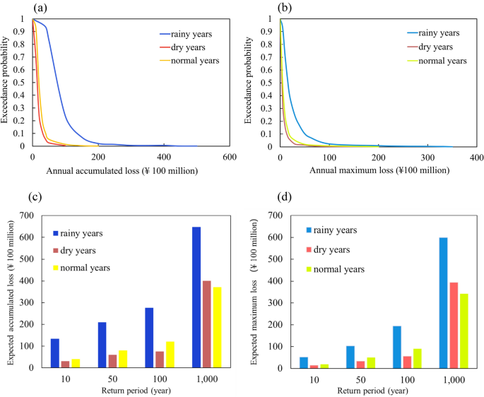
Aggregate exceedance probability (AEP) and occurrence exceedance probability (OEP) curves of the whole province of Hunan, China; and economic losses under different return periods: a AEP curve; b OEP curve; c expected accumulated loss under different return periods; d expected maximum loss under different return periods
-
(2)
Risk assessment for the northern and southern areas of Hunan Province
For the time coefficient of EOF2 of precipitation, the result is more complicated. Since the precipitation pattern corresponding to the time coefficient of EOF2 is a north-south opposite type, we discuss the southern and northern areas of the province separately. From the spatial distribution of the precipitation pattern, 27.5°N is roughly the north-south dividing line. Therefore, we define the area north of 27.5°N as the northern part, and the area south of the line is the southern part. Based on the time coefficient of EOF2 loading values, with ±0.5 standard deviation being used as the standard, the observed years are divided into three categories, corresponding to different regimes of precipitation. During the period from 1984 to 2007, the years when it was rainy in the north while dry in the south are: 1983, 1991, 1995, 1998, and 2003; the years when it was dry in the north while rainy in the south are: 1984, 1988, 1994, 1997, 2000, 2001, 2002, and 2006; the remaining years show normal precipitation for both the north and the south. The probability distributions of flooding frequency and economic losses are fitted. Similarly, according to the goodness-of-fit comparisons, the lognormal distribution provides the best fit for flooding frequency under each precipitation regime. The generalized extreme value distribution and normal distribution provide good fits for the flood economic losses in different data groups. We conducted the same procedures as described above for the whole province and obtained the AEP and OEP curves for the north and the south regions of Hunan Province separately.

In the northern area of the province, the AEP and OEP curves indicate a similar trend as those of the whole province: in rainy years, the flood losses are the most serious, and the flood losses are the lightest in dry years. The maximum loss of certain flooding events is very different from the annual accumulated loss in magnitude under several return periods. For example, when we consider a 1000-year return period condition, the maximum loss is approximately RMB 1.6 billion yuan, whereas the annual accumulated loss is approximately RMB 17 billion yuan, that is 10 times higher.
The AEP and OEP curves in the southern area similarly obey the same rules. However, there is a similarity in the magnitudes of maximum loss and annual accumulated loss under each return period in the southern area, which is very different from the condition in the northern area. This finding is unexpected and very interesting, because logically the accumulated loss should be larger than the maximum loss. Considering the spatially unbalanced economic development in Hunan, especially between the northern and southern areas, we make a rough comparison of flood risk variations in these two areas and analyze the potential reason for this result.
According to the China Statistical Yearbook and the local government report, there is a difference in the economic development between the northern and southern areas in Hunan Province. The northern area includes the Changsha, Zhuzhou, Xiangtan core-city group, which is more economically developed than other areas of the province. From the governmental statistical data, the population in the Changsha, Zhuzhou, Xiangtan core-city group accounts for around 60% of the total population of the province and the per capita GDP of this area is 1.4 times higher than the provincial average. In the southern area of Hunan, the population accounts for 26.9% of the provincial total, and the area contributes 20.4% of the GDP of the whole province (data in 2010).Footnote 1
Figure 7 indicates that in terms of the expected maximum loss, when less serious flooding occurs (with a smaller return period), there is little difference between the two areas. But in the case of catastrophes (larger return period), the related economic losses are much larger in the southern area than in the northern area.

Occurrence exceedance probability (OEP) curves and annual maximum economic loss from flood events under different return periods (from left to right: rainy years, normal years, and dry years) for Hunan Province, China
Figure 8 shows the result of the annual accumulated loss, which is the opposite of the maximum loss result. The southern area suffers more serious maximum loss under the very extreme condition (larger return period). The annual accumulated loss is generally larger in the northern area. We can conclude that the southern area in Hunan Province tends to suffer more losses in a certain flood event, potentially due to its possibly weaker disaster management measures, whereas in the northern area the accumulated economic loss is more serious.

Aggregate exceedance probability (AEP) curves and annual accumulated economic losses from flood events under different return periods (from left to right: rainy years, normal years, and dry years) for Hunan Province, China
4 Conclusion
Flood risk assessment is essential for risk management. In this research, we propose a framework to connect climate factors and flood economic loss risk based on the spatial distribution and temporal variation of flood-season precipitation. We use Hunan Province in China to illustrate how our framework can be used and assess flood risk in Hunan Province, considering that this area is suffering from floods, which are largely influenced by the East Asia monsoon system and global climate change, as well as data accessibility. We find that:
-
1.
The estimated annual accumulated economic loss and maximum loss are more serious in rainy years, followed by normal years and dry years.
-
2.
Annual average loss (AAL) can be obtained by calculating the area of AEP curves, and AAL and estimated economic loss under different return periods can act as the estimation of economic loss risk.
-
3.
There is an obvious difference in flood risk between the northern area and southern area in Hunan Province. For the northern part, the maximum loss is much smaller than the cumulative loss under different return periods and each precipitation regime. In the southern area, these two types of losses are much closer to each other in magnitude.
-
4.
When we further compare the economic loss risks in these two areas, the results indicate that the maximum loss is always larger in the southern area compared with the northern region; however, for the accumulated loss, it is larger in the northern area except for the extreme condition (1000-year return period) under dry years. Economic development, the level of risk management, and the frequency of extreme weather events may be the reasons leading to this result.
-
5.
We have established a prediction model to forecast the time coefficients of EOFs of precipitation several months in advance, and the precipitation regime can be estimated for the next flood season according to our prediction model. We are able to obtain the flood economic loss risk for the whole province as well as separately for the northern and southern parts in the following year from the corresponding AEP and OEP curves, achieving the goal of assessing the flood risk with a lead time of several months.
Generally, we establish a framework using climate factors to predict the time coefficients of EOFs of precipitation and evaluate the economic loss risks under different precipitation regimes. We find that the flood risk differs under different rainfall regimes. Differences in population density and economic development in the northern and southern regions may be the reason that they suffer differently from disaster events with similar magnitude (same return period). The framework method proposed here can be used in regions suffering from flooding caused by extreme precipitation. The main purpose of this article is to introduce the framework and how it works in a region. The climate indices in the prediction model will change when applying this method to other regions, as different regions are influenced by different climate factors.
The limitation of this work arises from the fact that the relationship we explored between time coefficients of precipitation and climate factors is based on historical datasets; therefore, this relationship is relatively stationary. However, this relationship may vary with time (Wang et al. 2019; Yun et al. 2021), as some climate factors have been changing in recent decades and may continue to change in the future (Rodríguez-Fonseca et al. 2016). It is important to discuss how climate factors and related disaster events will change and estimate the related risk in the future. We estimate flood risk based on the historical economic loss data, which also change with socioeconomic development. As our framework can estimate flood risk several months in advance, it can be used as an early warning tool. We verify our precipitation forecast by using correlation and MSPE, while it is difficult to benchmark the estimated risk result.
Notes
https://tjj.hunan.gov.cn/hntj/tjfx/jczx/2011jczxbg/201507/t20150717_3788794.html (a government website, in Chinese)
References
Alexander, L.V., X. Zhang, T.C. Peterson, J. Caesar, B. Gleason, M. Haylock, D. Collins, B. Trewin, et al. 2006. Global observed changes in daily climate extremes of temperature and precipitation. Journal of Geophysical Research, 111(D5): Article D05109.
Almeira, G.J., and B. Scian. 2006. Some atmospheric and oceanic indices as predictors of seasonal rainfall in the Del Plata Basin of Argentina. Journal of Hydrology 329(1–2): 350–359.
Applequist, S., G.E. Gahrs, R.L. Pfeffer, and X.F. Niu. 2002. Comparison of methodologies for probabilistic quantitative precipitation forecasting. Weather and Forecasting 17(4): 783–799.
Arunraj, N.S., S. Mandal, and J. Maiti. 2013. Modeling uncertainty in risk assessment: An integrated approach with fuzzy set theory and Monte Carlo simulation. Accident Analysis & Prevention 55: 242–255.
Chang, Y.S., D. Jeon, H. Lee, H.S. An, J.W. Seo, and Y.H. Youn. 2004. Interannual variability and lagged correlation during strong El Niño events in the Pacific Ocean. Climate Research 27(1): 51–58.
Chen, W., J. Feng, and R. Wu. 2013. Roles of ENSO and PDO in the link of the East Asian winter monsoon to the following summer monsoon. Journal of Climate 26(2): 622–635.
Dai, Y., and B. Tan. 2019. On the role of the eastern Pacific teleconnection in ENSO impacts on wintertime weather over East Asia and North America. Journal of Climate 32(4): 1217–1234.
Dong, W. 2002. Engineering models for catastrophe risk and their application to insurance. Earthquake Engineering and Engineering Vibration 1(1): 145–151.
Doocy, S., A. Daniels, S. Murray, and T.D. Kirsch. 2013. The human impact of floods: A historical review of events 1980–2009 and systematic literature review. PLoS Currents. https://doi.org/10.1371/currents.dis.f4deb457904936b07c09daa98ee8171a.
Duan, D.Y., Y.X. Chen, and J.L. Ju. 1999. Discussion on the division and variation of precipitation in flood season in Hunan Province. Resources and Environment in the Yangtze River Basin 8: 440–444 (in Chinese).
Emerton, R., H.L. Cloke, E.M. Stephens, E. Zsoter, S.J. Woolnough, and F. Pappenberger. 2017. Complex picture for likelihood of ENSO-driven flood hazard. Nature Communications 8(1): 1–9.
Gao, T., and L. Xie. 2014. Multivariate regression analysis and statistical modeling for summer extreme precipitation over the Yangtze River basin China. Advances in Meteorology. https://doi.org/10.1155/2014/269059.
Goddard, L., and M. Dilley. 2005. El Niño: catastrophe or opportunity. Journal of Climate 18(5): 651–665.
Hisamatsu, R., S. Kim, and S. Tabeta. 2019. Estimation of expected loss by storm surges along Tokyo Bay coast. In Proceedings of the International Conference on Ocean, Offshore and Arctic Engineering, OMAE2019-95336, V009T13A005. 9−14 June 2019, Glasgow, Scotland.
Hiwasaki, L., E. Luna, and R. Shaw. 2014. Process for integrating local and indigenous knowledge with science for hydro-meteorological disaster risk reduction and climate change adaptation in coastal and small island communities. International Journal of Disaster Risk Reduction 10: 15–27.
Hsu, W.K., P.C. Huang, C.C. Chang, C.W. Chen, D.M. Hung, and W.L. Chiang. 2011. An integrated flood risk assessment model for property insurance industry in Taiwan. Natural Hazards 58(3): 1295–1309.
Hussung, S., S. Mahmud, A. Sampath, M. Wu, P. Guo, and J. Wang. 2019. Evaluation of data-driven causality discovery approaches among dominant climate modes. http://hpcf-files.umbc.edu/research/papers/CT2019Team2.pdf. Accessed 4 Sept 2021.
IPCC (Intergovernmental Panel on Climate Change). 2018. Global warming of 1.5°C. An IPCC special report on the impacts of global warming of 1.5°C above pre-industrial levels and related global greenhouse gas emission pathways, in the context of strengthening the global response to the threat of climate change, sustainable development, and efforts to eradicate poverty, ed. V. Masson-Delmotte, P. Zhai, H.-O. Pörtner, D. Roberts, J. Skea, P.R. Shukla, A. Pirani, W. Moufouma-Okia, et al. https://www.ipcc.ch/site/assets/uploads/sites/2/2019/06/SR15_Full_Report_Low_Res.pdf. Accessed 29 Sept 2021.
Jia, J.Y., Y. Wang, Z.B. Sun, Y. Liu, and H.S. Chen. 2010. Leading spatial patterns of summer rainfall quasibiennial oscillation and characteristics of meteorological backgrounds over eastern China. Chinese Journal of Geophysics 53(5): 740–749.
Jongman, B., S. Hochrainer-Stigler, L. Feyen, J.C. Aerts, R. Mechler, W.W. Botzen, L.M. Bouwer, and G. Pflug et al. 2014. Increasing stress on disaster-risk finance due to large floods. Nature Climate Change 4(4): 264–268.
Kelman, I., J.C. Gaillard, and J. Mercer. 2015. Climate change’s role in disaster risk reduction’s future: Beyond vulnerability and resilience. International Journal of Disaster Risk Science 6(1): 21–27.
Kiem, A.S., S.W. Franks, and G. Kuczera. 2003. Multi-decadal variability of flood risk. Geophysical Research Letters. https://doi.org/10.1029/2002GL015992.
Kundzewicz, Z.W., M. Szwed, and I. Pińskwar. 2019. Climate variability and floods—A global review. Water 11(7): Article 1399.
Li, S., J. Lu, G. Huang, and K. Hu. 2008. Tropical Indian Ocean basin warming and East Asian summer monsoon: A multiple AGCM study. Journal of Climate 21(22): 6080–6088.
Liu, X.F., H.Z. Yuan, and Z.Y. Guan. 2009. Effects of ENSO on the relationship between IOD and summer rainfall in China. Journal of Tropical Meteorology 15(1): 59–62.
Liu, Z., F. Zhang, Y. Zhang, J. Li, X. Liu, G. Ding, C. Zhang, Q. Liu, and B. Jiang. 2018. Association between floods and infectious diarrhea and their effect modifiers in Hunan province, China: A two-stage model. Science of the Total Environment 626: 630–637.
Lu, S., X. Zhang, H. Peng, M. Skitmore, X. Bai, and Z. Zheng. 2021. The energy-food-water nexus: Water footprint of Henan-Hubei-Hunan in China. Renewable and Sustainable Energy Reviews 135: Article 110417.
Ludescher, J., A. Gozolchiani, M.I. Bogachev, A. Bunde, S. Havlin, and H.J. Schellnhuber. 2014. Very early warning of next El Niño. Proceedings of the National Academy of Sciences 111(6): 2064–2066.
McPhaden, M.J., S.E. Zebiak, and M.H. Glantz. 2006. ENSO as an integrating concept in earth science. Science 314(5806): 1740–1745.
Munich Re. 2019. Natural catastrophe review, 2018. Munich Re, 8 January 2019.
Ning, L., and R.S. Bradley. 2014. Winter precipitation variability and corresponding teleconnections over the northeastern United States. Journal of Geophysical Research: Atmospheres 119(13): 7931–7945.
Nobre, G.G., B. Jongman, J.C.J.H. Aerts, and P.J. Ward. 2017. The role of climate variability in extreme floods in Europe. Environmental Research Letters 12(8): Article 084012.
North, G.R., T.L. Bell, R.F. Cahalan, and F.J. Moeng. 1982. Sampling errors in the estimation of empirical orthogonal functions. Monthly Weather Review 110(7): 699–706.
O’Donnell, E.C., and C.R. Thorne. 2020. Drivers of future urban flood risk. Philosophical Transactions of the Royal Society A 378(2168): Article 20190216.
Raikes, J., T.F. Smith, C. Jacobson, and C. Baldwin. 2019. Pre-disaster planning and preparedness for floods and droughts: A systematic review. International Journal of Disaster Risk Reduction 38: Article 101207.
Rodríguez-Fonseca, B., R. Suárez-Moreno, B. Ayarzagüena, J. López-Parages, I. Gómara, J. Villamayor, E. Mohino, T. Losada, et al. 2016. A review of ENSO influence on the North Atlantic. A non-stationary signal. Atmosphere 7(7): Article 87.
Royse, K.R., J.K. Hillier, L. Wang, T.F. Lee, J. O’Niel, A. Kingdon, and A. Hughes. 2014. The application of componentised modelling techniques to catastrophe model generation. Environmental Modelling & Software 61: 65–77.
Ruiz, J.E., I. Cordery, and A. Sharma. 2005. Integrating ocean subsurface temperatures in statistical ENSO forecasts. Journal of Climate 18(17): 3571–3586.
Shi, H., and B. Wang. 2019. How does the Asian summer precipitation-ENSO relationship change over the past 544 years?. Climate Dynamics 52(7): 4583–4598.
Stapleford, T.A. 2009. The cost of living in America: A political history of economic statistics. Cambridge: Cambridge University Press.
Stephenson, D.B., A. Hunter, B. Youngman, and I. Cook. 2018. Towards a more dynamical paradigm for natural catastrophe risk modeling. In Risk modeling for hazards and disasters, ed. G. Michel, 63–77. Amsterdam: Elsevier.
Steptoe, H., S.E.O. Jones, and H. Fox. 2018. Correlations between extreme atmospheric hazards and global teleconnections: Implications for multihazard resilience. Reviews of Geophysics 56(1): 50–78.
Tabari, H. 2020. Climate change impact on flood and extreme precipitation increases with water availability. Scientific Reports 10(1): 1–10.
Tabari, H., and P. Willems. 2018. Lagged influence of Atlantic and Pacific climate patterns on European extreme precipitation. Scientific Reports 8(1): 1–10.
Tao, F., M. Yokozawa, Z. Zhang, Y. Hayashi, H. Grassl, and C. Fu. 2004. Variability in climatology and agricultural production in China in association with the East Asian summer monsoon and El Niño Southern Oscillation. Climate Research 28(1): 23–30.
Tomozeiu, R., S. Stefan, and A. Busuioc. 2005. Winter precipitation variability and large-scale circulation patterns in Romania. Theoretical and Applied Climatology 81(3): 193–201.
Torgersen, G., J.T. Bjerkholt, K. Kvaal, and O.G. Lindholm. 2015. Correlation between extreme rainfall and insurance claims due to urban flooding — Case study Fredrikstad, Norway. Journal of Urban and Environmental Engineering 9(2): 127–138.
Tozer, C.R., A.S. Kiem, and D.C. Verdon-Kidd. 2017. Large-scale ocean-atmospheric processes and seasonal rainfall variability in South Australia: Potential for improving seasonal hydroclimatic forecasts. International Journal of Climatology 37(S1): 861–877.
Wang, L., and W. Chen. 2014. An intensity index for the East Asian winter monsoon. Journal of Climate 27(6): 2361–2374.
Wang, N., and Y. Zhang. 2015. Evolution of Eurasian teleconnection pattern and its relationship to climate anomalies in China. Climate Dynamics 44(3–4): 1017–1028.
Wang, B., J.Y. Lee, I.S. Kang, J. Shukla, C.K. Park, A. Kumar, J. Schemm, and S. Cocke et al. 2009. Advance and prospectus of seasonal prediction: assessment of the APCC/CliPAS 14-model ensemble retrospective seasonal prediction (1980–2004). Climate Dynamics 33(1): 93–117.
Wang, Y., Z. Li, Z. Tang, and G. Zeng. 2011. A GIS-based spatial multi-criteria approach for flood risk assessment in the Dongting Lake region, Hunan, central China. Water Resources Management 25(13): 3465–3484.
Wang, B., X. Luo, Y.M. Yang, W. Sun, M.A. Cane, W. Cai, S.W. Yeh, and J. Liu. 2019. Historical change of El Niño properties sheds light on future changes of extreme El Niño. Proceedings of the National Academy of Sciences 116(45): 22512–22517.
Wang, B., X. Luo, and J. Liu. 2020. How robust is the Asian precipitation-ENSO relationship during the industrial warming period (1901–2017)?. Journal of Climate 33(7): 2779–2792.
Wang, S.Y.S., W.R. Huang, H.H. Hsu, and R.R. Gillies. 2015. Role of the strengthened El Niño teleconnection in the May 2015 floods over the southern Great Plains. Geophysical Research Letters 42(19): 8140–8146.
Ward, P.J., B. Jongman, M. Kummu, M.D. Dettinger, F.C.S. Weiland, and H.C. Winsemius. 2014. Strong influence of El Niño Southern Oscillation on flood risk around the world. Proceedings of the National Academy of Sciences 111(44): 15659–15664.
Wobus, C., P. Zheng, J. Stein, C. Lay, H. Mahoney, M. Lorie, D. Mills, and R. Spies et al. 2019. Projecting changes in expected annual damages from riverine flooding in the United States. Earth’s Future 7(5): 516–527.
World Bank. 2017. Santa Catarina: Disaster risk profiling for improved natural hazards resilience planning. Washington, DC: World Bank.
Wu, Z., B. Wang, J. Li, and F.F. Jin. 2009. An empirical seasonal prediction model of the East Asian summer monsoon using ENSO and NAO. Journal of Geophysical Research Atmospheres. https://doi.org/10.1029/2009JD011733.
Xiao, J., M. Wang, L. Tian, and Z. Zhen. 2018. The measurement of China’s consumer market development based on CPI data. Physica A: Statistical Mechanics and its Applications 490: 664–680.
Xiao, M., Q. Zhang, and V.P. Singh. 2015. Influences of ENSO, NAO, IOD and PDO on seasonal precipitation regimes in the Yangtze River basin. China. International Journal of Climatology 35(12): 3556–3567.
Yavuz, H., and S. Erdoğan. 2012. Spatial analysis of monthly and annual precipitation trends in Turkey. Water Resources Management 26(3): 609–621.
Yun, K.S., J.Y. Lee, A. Timmermann, K. Stein, M.F. Stuecker, J.C. Fyfe, and E.S. Chung. 2021. Increasing ENSO-rainfall variability due to changes in future tropical temperature–rainfall relationship. Communications Earth & Environment 2(1): 1–7.
Zebiak, S.E., B. Orlove, Á.G. Muñoz, C. Vaughan, J. Hansen, T. Troy, M.C. Thomson, A. Lustig, and S. Garvin. 2015. Investigating El Niño-Southern Oscillation and society relationships. Wiley Interdisciplinary Reviews: Climate Change 6(1): 17–34.
Zhao, J., L. Yang, and G. Feng. 2018. Circulation system configuration characteristics of four rainfall patterns in summer over the East China. Theoretical and Applied Climatology 131(3): 1211–1219.
Zhou, Z.Q., S.P. Xie, and R. Zhang. 2021. Historic Yangtze flooding of 2020 tied to extreme Indian Ocean conditions. Proceedings of the National Academy of Sciences 118(12): Article e2022255118.
Acknowledgement
This research was partially supported by the National Natural Science Foundation of China (grant No. 41671503).
Author information
Authors and Affiliations
Corresponding author
Rights and permissions
Open Access This article is licensed under a Creative Commons Attribution 4.0 International License, which permits use, sharing, adaptation, distribution and reproduction in any medium or format, as long as you give appropriate credit to the original author(s) and the source, provide a link to the Creative Commons licence, and indicate if changes were made. The images or other third party material in this article are included in the article's Creative Commons licence, unless indicated otherwise in a credit line to the material. If material is not included in the article's Creative Commons licence and your intended use is not permitted by statutory regulation or exceeds the permitted use, you will need to obtain permission directly from the copyright holder. To view a copy of this licence, visit http://creativecommons.org/licenses/by/4.0/.
About this article

Cite this article
Hu, X., Wang, M., Liu, K. et al. Using Climate Factors to Estimate Flood Economic Loss Risk. Int J Disaster Risk Sci 12, 731–744 (2021). https://doi.org/10.1007/s13753-021-00371-5
Accepted:
Published:
Issue Date:
DOI: https://doi.org/10.1007/s13753-021-00371-5