Application of hydraulic flow units’ approach for improving reservoir characterization and predicting permeability

Abstract

It is highly essential to characterize the reservoir accurately as possible to implement enhanced oil recovery and development scenarios. Determining complex variations in pore geometry aids in identifying rock types with similar fluid flow properties. Traditional classification of rock types is based on geologic observations and empirical relations between porosity and permeability. However, for a given porosity, permeability can vary by several orders of magnitude. This reveals that porosity only cannot interpret the permeability variation. The proposed approach to define the existence of different rock types in the reservoir is the “hydraulic flow units’ approach.” The approach aims to enhance the reservoir characterization and predict permeability in un-cored wells to reduce the cost of drilling core samples. The approach involves dividing the reservoir into hydraulic flow units (HFUs). It introduces the concept of reservoir quality index and flow zone indicator (FZI) to identify the HFUs. Each unit is imprinted by certain FZI and said to have similar geological and petro-physical properties. Validation of results was done by integrating the HFUs with core description results—particularly samples’ grain sizes—to ascertain the accuracy of the approach. FZI was then integrated with well logs using multiple regression analysis in order to train the logs to recognize the hydraulic flow units in case of absence of core. A regression model was developed for each flow unit, from which FZI can be estimated from logs only. FZI was then correlated with permeability to compute permeability. Results showed that four HFUs exist in the reservoir. Four categories of grain sizes were identified from core analysis. This emphasized the accuracy of the proposed technique. Besides, integration between core data and well-logging ones showed high degree of correlation between well logs and FZI. Expanding this correlation aids in predicting permeability in un-cored well.

Introduction

In the upstream petroleum industry, reservoir characterization plays an important role in giving geologists and reservoir engineers a more accurate and detailed understanding of the subsurface reservoir. Understanding key reservoir properties such as pore geometry, tortuosity, and permeability assists geologists and reservoir engineers in improving the characterization of the reservoir and enhancing its performance and development throughout its lifetime.

Traditionally, several investigators have proposed that permeability can be estimated from a linear regression model, assuming that a linear relationship exists between core porosity and permeability (Busch et al. 1987; Canas et al. 1994). This method ignores the scatter of data, assuming that it is due to measurement errors. Moreover, it ignores the fact that there is no theoretical basis for a relationship between porosity and permeability; as high and low permeability zones with equal porosity values may exist in the same reservoir. In addition to that, fractured limestone can constitute low porosity with high permeability. Consequently, many investigators noted the inadequacy of this classical approach and demonstrated that permeability is not only dependent on porosity, but also dependent on other depositional characteristics such as grain size, pore geometry, tortuosity, which is affected by diagenetic factors such as cementation, fracturing and solution. As a result, a better approach to improve the characterization of the reservoir, taking into account the fundamentals of geology and physics of flow at porous media, is needed. This will attribute the interdependency between permeability and geological variations in the reservoir rock. The proposed approach to do this is the hydraulic flow units’ approach.

Location of the study area

The proposed approach was applied at JG field. JG field is an E-W field discovered in the West of North East of Abu El-Gharadig basin (NEAG concession) in 2001, where Shell Company achieved a commercial discovery from the Jurassic play there. The field is located between longitudes 28°06′ to 28°17′E and between latitudes 30° to 30°34′N. As shown in Fig. 1: JG field lies some 35 km NW of Bed 1 oil field, 35 km NE of Bed 3 gas Field, 25 km NE of Bed 16/17 oil fields. Its total area is about 100.17 km². The approach was applied to three cored wells and one un-cored one in the field.

Fig. 1

Location map of JG field

Petroleum system at the field

JG field comprises the elements of petroleum system, represented in source rock, reservoir rock, migration, trapping and sealing. Khatatba Formation is considered as the main source rock in JG field. Khatatba Formation is Middle Jurassic in age. Underneath it is Ras Qattara formation and above it is Masajid Limestone as shown in Fig. 2. It is composed of four distinctive lithological members: Lower Safa Member at the bottom; Kabrit Member, Upper Safa Member, and Zahra Member at the top. Khatatba Formation indicates a remarkable variation in facies coincided with a remarkable variation in thickness (Moustafa 2008).

Fig. 2

Generalized stratigraphic column of the Western Desert (Shalaby et al. 2013)

Khataba organic shale and coaly shale (Lower Safa A and B Members) are the main source rocks at the field, with high total organic carbon (TOC) amount. Kerogen is of mixed type II–III, which is capable of generating oil and gas (El-Kader 2016).

Sandstone of Lower Safa A and C Members is the main reservoir rock in JG field. Migration takes place across normal fault structures formed during Jurassic rifting. Shale and compact limestone of Kabrit and Zahra members with Masajid Limestone is the main seal.

Theory of hydraulic flow units (HFUs)

The need of defining quasi-geological/engineering units has been recognized by petroleum geologists and engineers to shape the description of reservoir zones as storage containers and reservoir conduits for fluid flow. Flow units are resultant of depositional environment and diagenetic processes. Bear (2013) defined the hydraulic flow unit as the representative elementary volume of the total reservoir rock within which geological and petro-physical properties are the same. These properties are similar in the same flow unit but differ from one unit to another. Porosity and permeability are two key parameters that influence the flow in the reservoir. They can be measured directly by core analysis. In case of absence of a core, indirect methods must be used. Kozeny (1927) and Carman (1937) developed an equation to estimate permeability, where:

$$K = \left( {\frac{1}{{2 \cdot T^{2} \cdot S_{{{\text{v}}_{\text{gr}} }}^{2} }}} \right)*\left( {\frac{{\varPhi^{3} }}{{(1 - \varPhi )^{2} }}} \right)$$

(1)

where k permeability (µm²), T tortuosity of the flow path, $S_{{{\text{v}}_{\text{gr}} }}$: specific surface area per unit grain volume, Φ: effective porosity, fraction.

The factor 2 in Eq. 1 accounts for the assumption that pores are cylindrical. In reality, this is not always the case as pore shape can vary across the reservoir from one unit to another. So, a modification has been developed to the basic model by considering the pore shape as follows:

$$K = \left( {\frac{1}{{F_{\text{s}} \cdot T^{2} \cdot S_{{{\text{v}}_{\text{gr}} }}^{2} }}} \right)*\left( {\frac{{\varPhi^{3} }}{{(1 - \varPhi )^{2} }}} \right)$$

(2)

where $F_{\text{s}}$ is the pore shape factor. Table 1 indicates the shape factors for different pore shapes.

Table 1 Kozeny shape factor F_s (Schön 2015)

where (a) of an ellipse is the distance from the centre to the ellipse along the major axis and (b) is the distance from the centre to ellipse along the minor axis as shown in Fig. 3, whilst (a) of a rectangle is its length and (b) is its width. Different values of (a/b) for ellipse and rectangle are shown in the second column of Table 1, where there is a certain shape factor for each value of (a/b).

Fig. 3

Ellipse with its shape parameters

where (c) is the linear eccentricity.

The term $(F_{\text{s}} \cdot T^{2} \cdot S_{{{\text{V}}_{\text{gr}} }} )$ is a function of the geological characteristics of porous media. It varies with changes in pore geometry. The discrimination of this term is the basis of hydraulic unit classification technique. The term $(F_{\text{s}} \cdot T^{2} )$ is the Kozeny constant. It describes the shape and geometry of the pore channels and usually has a value between 5 and 100 in most reservoir rocks (Tiab and Donaldson 2015)

Kozeny constant varies between flow units, but is constant in a given unit. Amaefule et al. (1993) addressed the variability of the Kozeny constant by dividing Eq. 2 by porosity and taking square root of both sides. This yields:

$$\sqrt {\frac{K}{\varPhi }} = \frac{1}{{\sqrt {F_{\text{s}} } \cdot T \cdot S_{{{\text{v}}_{\text{gr}} }} }} \cdot \frac{\varPhi }{1 - \varPhi }$$

(3)

$${\text{where}}\quad \varPhi = \frac{\varPhi }{1 - \varPhi }$$

(4)

$\phi_{z}$ is the ratio of pore volume to grain volume and is known as the normalized porosity.

If permeability is expressed in millidarcies, the reservoir quality index (RQI) parameter can be defined as follows:

$${\text{RQI}} = \pi *10^{ - 2} *\sqrt {\frac{K}{\varPhi }}$$

(5)

where RQI is expressed in micrometres (µm).

Flow zone indicator (FZI) parameter can be defined from Eq. 3 as:

$${\text{FZI}} = \frac{1}{{\sqrt {F_{\text{s}} } \cdot T \cdot S_{{{\text{v}}_{\text{gr}} }} }}$$

(6)

FZI parameter integrates the geologic attributes of texture and mineralogy in the discrimination of hydraulic flow units. Rocks containing fine-grained, poorly sorted sands with authigenic pore bridging clays tend to exhibit high surface area and high tortuosity and hence low FZI. On the other hand, rocks containing coarse-grained, well-sorted sands exhibit lower surface area and lower tortuosity and hence high FZI.

Substituting Eqs. 4, 5, 6 in Eq. 3 results in:

$${\text{RQI}} = {\text{FZI}}*\phi_{z}$$

(7)

Taking logarithm for both sides of Eq. (7) yields:

$${\text{Log}}\,{\text{RQI}} = { \log }\,{\text{FZI}} + { \log }\,\phi_{z}$$

(8)

Combining Eqs. 5 and 7 yields:

$$K = 1014*({\text{FZI}})^{2} *\frac{{\phi^{3} }}{{(1 - \phi )^{2} }}$$

(9)

The permeability of a sample point can be calculated from the above equation using mean value of FZI and the corresponding sample porosity.

Data processing

A plot of porosity and logarithm of permeability obtained from conventional core analysis of three cored wells in JG field is indicated in Fig. 4, where the conventional form of permeability as a function of porosity is:

Fig. 4

Cross-plot of porosity versus log permeability of the studied cored wells

$${\text{Log}}\,K = a + m\varphi$$

(10)

The figure shows a lot of scatter and some samples of same porosity but different permeability values. This reveals a fact that porosity is not the only parameter that can explain permeability variation. This can be attributed to the existence of more than one rock type (HFU) in the reservoir, where each rock type has fluid flow properties different from the other. Subsequently, better correlation can be obtained if rocks with similar fluid flow properties are identified and grouped together.

Several approaches can be used for clustering core data into HFUs. One of which is the histogram analysis. FZI is strongly dependent on permeability and usually exhibits log-normal distribution. As a result, clustering of FZI is performed on biases of logarithm of FZI. When clusters are distinctly separated, the histogram can delineate each HFU. A histogram of log FZI of the studied cored wells is shown in Fig. 5.

Fig. 5

Histogram of log FZI of the studied cored wells

The figure indicates that it is difficult to separate the overlapped distributions as the transition zones between different HFUs cloud the judgment on their identity. Consequently, histogram is not the appropriate approach.

A second approach is the normal probability plot (cumulative distribution function). It is the integral of probability density function (histogram). It can be used to determine the number of HFUs since a normal distribution forms a distinct straight line on the plot. The number of straight lines indicates the number of HFUs in the reservoir. A probability plot of log FZI of the studied cored wells is shown in Fig. 6.

Fig. 6

Probability plot of log FZI of the studied cored wells

The figure shows less data scatter than the histogram. However, exact number of HFUs cannot be determined due to the superposition effect that may shift or distort the straight lines.

The third approach is the iterative multi-linear regression (IMLR) clustering technique discussed by Al-Ajmi and Holditch (2000), where core data can be used to identify the hydraulic flow units in the reservoir through the following procedures:

• 1. Select core data and compute $\varphi_{z}$ and RQI (Eqs. 4 and 5).

• 2. Plot log $\varphi_{z}$ versus log RQI (Fig. 7).

  Fig. 7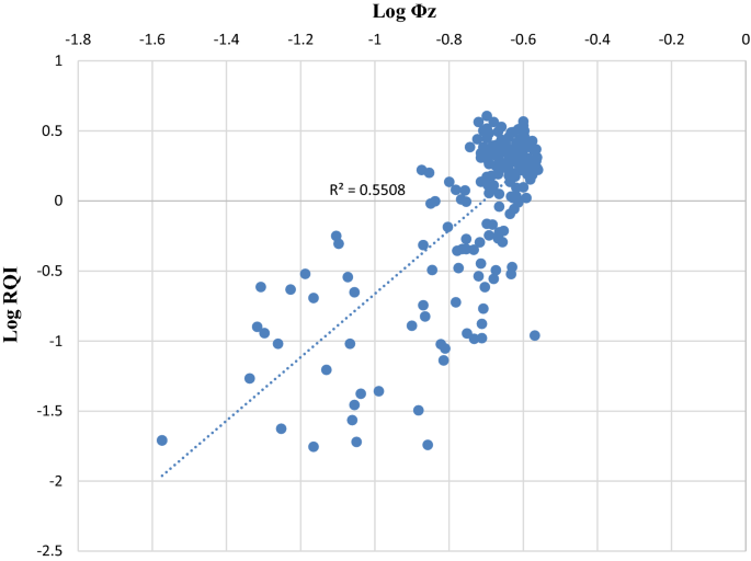

  

  Cross-plot of log-normalized porosity versus log reservoir quality index of core data

• 3. Use an initial reasonable guess of each straight line’s intercept (mean FZI).

• 4. Allocate core sample data to the nearest straight line.

• 5. Recalculate the intercept of HFU using least-square regression equations.

• 6. Compare the old and new values of each straight line’s intercept. If the difference is not within the acceptable tolerance, update the intercept values and go to step 3.

The basis of hydraulic unit classification is identifying group of data samples that achieve unit slope straight lines on the plot as shown in Fig. 8.

Fig. 8

Clustering core data into the optimal number of HFUs using IMLR technique

Figure 7 shows one HFU used to fit the data. The figure shows a lot of scatter with a coefficient of determination 0.5508.

Figure 8 indicates the existence of four hydraulic flow units in the reservoir. Each unit is represented by a straight line with a unit slope and mean FZI value. This reflects that each unit is precipitated at certain geological conditions and has fluid flow properties different from the other unit. The data scattered around the straight line are a result of measurement errors in core data analysis and minor fluctuations around main geological controls on pore throat characteristics of rock samples.

Validation of results

To validate the accuracy of the proposed technique, we validate the results by relating the HFUs to core description information, particularly sample grain size as permeability is strongly affected by sample grain size. Sedimentological analysis was performed to describe the existing cores in terms of lithology, cement, sorting and grain size. Core description results indicate the existence of four sandstone rock types in the reservoir as follows:

• 1. Light to dark grey, very-fine-to fine-grained, well-sorted, well-cemented, siliceous cement.

• 2. Grey, very-fine-to-medium-grained, medium-to-well-sorted, medium- to well-cemented, siliceous cement.

• 3. Light grey, fine-to-medium-grained, medium-to-well-sorted, siliceous cement.

• 4. Yellowish grey, medium-to-coarse-grained, medium-sorted, medium-cemented, siliceous cement.

FZI integration with well-logging data

Core data (represented in FZI) are integrated with well logs in order to train the logs to recognize the hydraulic flow units or the FZI. Integration process involves two procedures:

• 1. Core-log depth match.

• 2. Correlating HFU (FZI) with well logs via multiple regression analysis (MRA).

Core-log depth match

The logging tool was lowered on a cable in the subsurface to record certain formation feature. During pulling up the cable to surface, cable may be stretched and difference occurs between the depth where logging tool records the feature and the depth where the core sample was taken. Consequently, we must compute the difference between the two depths and apply the shift. Gamma ray log is the reference log, since the tool can run in both open and cased holes. GR log is correlated with the core gamma log. The core gamma log is a log created in the laboratory by moving the core past a gamma ray detector. The log can be either of the spectral response in weight concentrations of thorium, uranium and potassium, or of the total gamma ray in API units. Via Techlog software, we input the core gamma log in front of GR log, then determined the difference between the two depths and applied the shift as shown in Fig. 9.

Fig. 9

a Core and log depths before shift. b after shift

Figure 9 shows that depth shift at JG-3 well from depth 3281–3309 m is 4 m. The core-log depth match was applied at the whole cored wells.

The second step in the core-log integration is correlating the hydraulic flow unit (FZI) with the well logs via multiple regression analysis (MRA). Selection of corrected wire-line log data is based on their ability to reflect the pore space attributes.

The general form of multiple regression equation of Y on $X_{1} ,X_{2} ,X_{3} \ldots X_{n}$ is given by:

$$Y = b_{o} + b_{1} X_{1} + b_{2} X_{2} + \cdots + b_{n} X_{n}$$

(11)

where Y is the dependent variable (FZI), ($X_{\text{s}}$) are the independent variables [logging measurements; $x_{1}$ (density), $x_{2}$ (neutron), $x_{3}$ (gamma ray), $x_{4}$ (deep resistivity) and $x_{5}$ (shallow resistivity)], $b_{o} ,b_{1} , \ldots b_{n}$ are the regression coefficients.

Via Minitab software, we input dependent variable (FZI) and independent variables (well logs). In order to choose the best model, we input variables in linear, logarithmic and exponential forms and then the equation that achieves the highest correlation between different variables, and the least residual was chosen. A regression model was developed for each flow unit, where FZI can be computed from logs only $( {\text{FZI}}_{ \log } )$.

A cross-plot of ${\text{FZI}}_{\text{core}}$ versus ${\text{FZI}}_{ \log }$ of all reservoir HFUs is shown in Fig. 10, where correlation coefficient is 0.93 and hence indicates very strong correlation between the two parameters.

Fig. 10

Cross-plot of ${\text{FZI }}_{\text{core }}$ versus ${\text{FZI}}_{ \log }$ for all reservoir HFUs

Posteriorly, we applied Eq. 9 to compute permeability. Cross-plots of measured permeability from core versus calculated one for each HFU are shown in Figs. 11, 12, 13 and 14, where correlation coefficients are 0.92, 0.87, 0.88 and 0.78, respectively. This indicates strong correlation between calculated permeability and measured one.

Fig. 11

Cross-plot of measured permeability versus calculated one of HFU 1

Fig. 12

Cross-plot of measured permeability versus calculated one of HFU 2

Fig. 13

Cross-plot of measured permeability versus calculated one of HFU 3

Fig. 14

Cross-plot of measured permeability versus calculated one of HFU 4

Predicting permeability in un-cored well

There are different ranges of logging measurements (GR, density, neutron and resistivity) that characterize each flow unit. We related the promising un-cored interval to these logging ranges to determine to which HFU the un-cored interval belongs to. The following procedures have been followed to achieve this:

• 1. The promising area of the un-cored interval was selected from the composite log as shown in Fig. 15 (the area between the two black bold lines where low GR curve and crossover between neutron-density curves occur).

  Fig. 15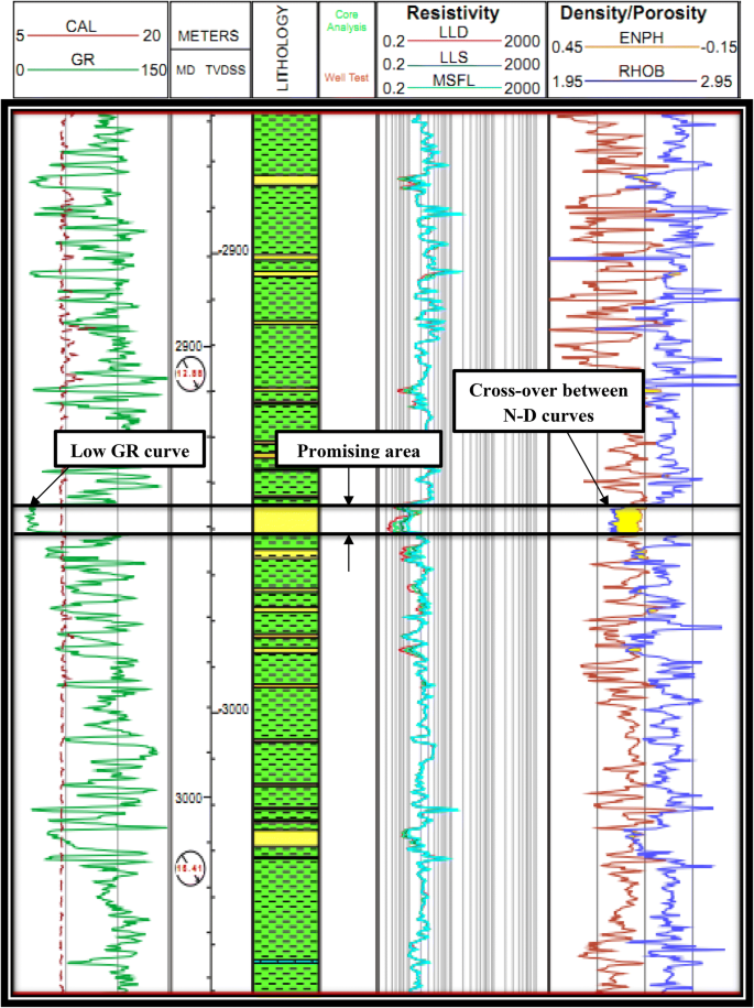

  

  Composite log at promising un-cored interval at JG-12 well

• 2. Logging measurements of the promising area were related to certain HFUs, according to the well-logging measurements’ ranges of previous classified HFUs.

• 3. The suitable regression equation of the flow unit was applied to compute the FZI.

• 4. Equation 9 is used to compute permeability.

We observed that the promising area is related to HFU 4. Consequently, the fourth regression equation was applied to compute FZI; thereafter, permeability is estimated using Eq. 9. Results are shown in Table 2.

Table 2 FZI and predicted permeability values at promising area at JG-12

Summary and conclusions

Routine core analysis data of three cored wells in JG field were used to compute normalized porosity and RQI for the cored sections. Representation of these data showed that the reservoir is composed of different flow units with different fluid flow properties. So, we cannot deal with the reservoir as one unit. Four hydraulic flow units were identified; each has its own FZI mean value. Core-log integration procedure was performed to create a relation between core data (FZI) and logging ones for each flow unit. Finally, expansion of this relation aids in predicting permeability in un-cored well. A flowchart of the procedures taken for predicting permeability in un-cored well is shown in Fig. 16.

Fig. 16

Flowchart of procedures for predicting permeability in un-cored wells

Based on the results of the case studied, we concluded that:

• 1. Hydraulic flow units’ approach is an accurate approach that has the ability to classify the reservoir into units relying on geological and petro-physical characteristics of each unit.

• 2. Combining geological attributes (included in FZI) with logging data is essential in order to train logs to identify HFUs determined from core data.

• 3. Multiple regression analysis is an effective statistical method that can correlate dependent variables (FZI) to independent ones (logging measurements). Expanding this correlation helps us in predicting permeability in un-cored well.

References

Al-Ajmi FA, Holditch SA (2000) SPE annual technical conference and exhibition. Society of Petroleum Engineers
Amaefule JO, Altunbay M, Tiab D, Kersey DG, Keelan DK (1993) SPE annual technical conference and exhibition. Society of Petroleum Engineers
Bear J (2013) Dynamics of fluids in porous media. Courier Corporation, Chelmsford
Busch J, Fortney W, Berry L (1987) Determination of lithology from well logs by statistical analysis. SPE Form Eval 2:412–418
Canas J, Malik Z, Wu C (1994) Permian basin oil and gas recovery conference. Society of Petroleum Engineers
Carman PC (1937) Fluid flow through granular beds. Trans Inst Chem Eng 15:150–166
El-Kader AA (2016) The use of seismic interpretations to discover and evaluate the new hydrocarbon prospects of Jurassic formations in JG field, NEAG concession, North Western Desert. J Pet Sci Eng 147:654–671
Kozeny J (1927) Über Kapillare Leitung des Wassers im Boden.-Sitzung Berichte Akad. Wiss., Wien, Nat
Moustafa A (2008) 3rd symposium on the sedimentary basins of Libya (The geology of East Libya). Earth Science Society of Libya, Tripoli, pp 29–46
Schön JH (2015) Physical properties of rocks: fundamentals and principles of petrophysics. Elsevier, Amsterdam
Shalaby MR, Hakimi MH, Abdullah WH (2013) Modeling of gas generation from the Alam El-Bueib formation in the Shoushan Basin, northern western Desert of Egypt. Int J Earth Sci 102:319–332
Tiab D, Donaldson EC (2015) Petrophysics: theory and practice of measuring reservoir rock and fluid transport properties. Gulf Professional Publishing, Houston
Author information
Authors and Affiliations
Corresponding author
Additional information
Publisher's Note
Springer Nature remains neutral with regard to jurisdictional claims in published maps and institutional affiliations.
Rights and permissions
Open Access This article is distributed under the terms of the Creative Commons Attribution 4.0 International License (http://creativecommons.org/licenses/by/4.0/), which permits unrestricted use, distribution, and reproduction in any medium, provided you give appropriate credit to the original author(s) and the source, provide a link to the Creative Commons license, and indicate if changes were made.
About this article
Cite this article
Khalid, M., Desouky, SD., Rashed, M. et al. Application of hydraulic flow units’ approach for improving reservoir characterization and predicting permeability. J Petrol Explor Prod Technol 10, 467–479 (2020). https://doi.org/10.1007/s13202-019-00758-7
Received:
Accepted:
Published:
Issue Date:
DOI: https://doi.org/10.1007/s13202-019-00758-7