
Abstract
Purpose
Current field emission modelling and toxicity characterisation of pesticides suffer from several shortcomings like mismatches between LCI databases and LCIA methods, missing characterisation factors, missing environmental compartments, and environmental impact pathways. The OLCA-Pest project was implemented to address these aspects and to operationalise the assessment of pesticides in LCA. Based on this effort, we propose an approach to integrate pesticide emissions into LCI databases.
Methods
The PestLCI Consensus Model has been developed in order to estimate emission fractions to different environmental compartments. The initial distribution fractions should be linked to the compartments air, agricultural soil, natural soil, and freshwater. Emissions to off-field surfaces are hereby distributed between agricultural soil, natural soil, and freshwater by using surface cover data. Deposition on the crop surface should be recorded in an emission compartment crop with 13 sub-compartments for crop archetypes for both food and non-food uses. Default emission fractions are provided to calculate the emission fractions for different pesticide application scenarios.
Results and discussion
A sensitivity analysis shows the effects of the application technique, drift reduction, crop and development stage, field width, and buffer zone on the initial distribution fractions of field-applied pesticides. Recommendations are given for the implementation of a set of default initial distribution fractions into LCI databases, for the organisation of metadata, and for the modelling of pesticide residues in food along the supply chain (processing, storage). Priorities for further research are: improving the modelling of pesticide secondary emissions, further extending emission modeling (e.g. additional application techniques, including cover crops), considering metal-based pesticides in emission models, and systematically assessing human health impacts associated with pesticide residues in food crops.
Conclusions
The proposed approach allows to preserve the mass balance of the pesticide emitted after application, to make a consistent assessment of ecotoxicity and human toxicity, to define a clear and consistent interface between the LCI and LCIA phases, to estimate initial emission distribution fractions based on existing data, to document metadata transparently and efficiently within crop datasets, and to model the removal of pesticide residues in food during processing.
1 Introduction
The widespread use of pesticides in agriculture has multiple impacts on the environment (Fantke 2019). It is therefore crucial that pesticides can be properly considered within life cycle assessment (LCA) studies in agriculture and the food sector. Due to the high uncertainty of toxicity impact results and the challenges related to the toxicity assessment of pesticides, many LCA studies in the agri-food sector do not perform an assessment of toxicity impacts of these compounds. This results in an incomplete assessment and bears the risk of overlooking potential hotspots and trade-offs. For example, a comprehensive meta-study of agri-food LCA by Poore and Nemecek (2018) could not successfully collect a sufficient amount of consistent LCA data on ecotoxicity, due the scarcity of studies reporting ecotoxicity impacts and lack of harmonisation of methodology. Current field emission modelling and toxicity characterisation of pesticides suffer from several shortcomings. Clear rules are lacking to distinguish between what matters for the inventory (LCI) of pesticide emissions to environmental compartments (air, soil, and water), and what matters for the fate of pesticides (i.e. degradation and transfers between compartments), which is supposed to be taken into account in the life cycle impact assessment models (LCIA, van Zelm et al. 2014; Rosenbaum et al. 2015). However, models used in impact assessment are of generic nature, which means that the effects of agricultural practices on emissions (e.g. buffer zones on field boundaries), application techniques (e.g. anti-drift nozzles), or local soil and climate conditions are usually not considered (Gentil et al. 2020b).
Databases like ecoinvent (Wernet et al. 2016) or the World Food Life Cycle Database (Nemecek et al. 2015) currently model pesticide emissions as equal to the amount applied, which is — due to lacking alternatives — counted as a direct emission exclusively to agricultural soil. Current category rules are suggesting fixed proportion of emissions (e.g. 90% soil, 9% air, 1% water, European Commission 2019). Toxicity impact assessment methods, however, assume that the emissions to the different environmental compartments are calculated in the inventory phase, which creates potential inconsistencies. In addition, LCA practitioners in agriculture are currently facing the challenge that no impact assessment method covers characterisation factors for all pesticides. As calculating characterisation factors is often too demanding and out of scope of a study, the impacts of such substances are either ignored, or replaced by a proxy value, which considerably increases the uncertainty. In fact, a major portion of a pesticide applied is often deposited on the crop itself. However, we have no corresponding environmental compartment in the impact assessment, so that there is a risk of ignoring related environmental impacts. This poses a particular problem for assessing the impacts of pesticide residues on food, which can e.g. be done by the dynamiCROP model (Fantke et al. 2011a, b). Moreover, some environmental impact pathways are missing, like farming occupational exposure, and residential and non-residential bystanders’ exposure (Fantke 2019). Finally, even if methods for the assessment of direct intake of pesticide via residues on food products have been developed (Fantke and Jolliet 2016), their application in standard LCAs is still facing many obstacles.
In the absence of an easy-to-use consensual approach, most users make the simplifying assumption that 100% of the dose per hectare of pesticide is emitted to the soil or follow simplifying approaches that distribute pesticide emissions (using fixed percentages) on more than one environmental compartment (Berthoud et al. 2011; Margni et al. 2002; Neto et al. 2013). The impact model then calculates the redistribution between air, soil, and water on a macroscopic temporal and spatial scale as illustrated in Fig. 1. On the other hand, more sophisticated models, such as PestLCI version 1 (Birkved et al. 2006) and 2 (Dijkman et al. 2012), estimate emissions to three environmental compartments: air, surface water, and groundwater. PestLCI has been used in various LCA studies (Vazquez-Rowe et al. 2012; Nordborg et al. 2014; Renaud-Gentié et al. 2015; Fantin et al. 2016), but these applications are highly specific and a harmonisation is lacking. In addition, some of these studies took into account the degradation of pesticides over long periods of time, which led to a double counting of these phenomena with LCIA models (Van Zelm et al. 2014).

Modelling of pesticides in LCA before and after the contribution of the OLCA-Pest project
To cope with these challenges, a consensus process was initiated with three scientific workshops (2013 in Glasgow, 2014 in Basel, 2015 in Bordeaux) and a stakeholder workshop (2016 in Dublin), which defined the theoretical framework for pesticide emission modelling (Rosenbaum et al. 2015; Fantke et al. 2017). In order to operationalise and harmonise the emission quantification and impact characterisation of pesticides in LCA and product environmental footprinting (PEF) based on this effort, the OLCA-Pest project “Operationalising Life Cycle Assessment for Pesticides”, 2017–2020, co-funded by ADEME, https://orbit.dtu.dk/en/projects/olca-pest) was implemented with nine partner institutions. Based on the analysis of potential gaps and overlaps between the inventory and impact phases, the PestLCI 2.0 model (Dijkman et al. 2012) was further developed into a consensus version for pesticide emission modelling (Fantke et al. 2017) and operationalised on a web-based platform (https://pestlciweb.man.dtu.dk). Combining it with the dynamiCROP plant uptake model for human exposure and toxicity characterisation with special focus on pesticide residues in food crops (Fantke et al. 2011a, b; Gentil et al. 2020a), and the USEtox scientific consensus model for human toxicity and ecotoxicity characterisation (Rosenbaum et al. 2008; Fantke et al. 2021), we propose a solution for the integration of pesticide emissions into LCI databases, in order to provide a consistent emission and impact modelling for pesticides in LCA as shown in the bottom part of Fig. 1.
This paper summarises the recommendations from the OLCA-Pest project regarding the implementation of the pesticide consensus in LCI databases and LCA software and the consequences for the impact assessment for users modelling generic impacts of pesticides and for background datasets. We start with giving an overview of the different application cases (Sect. 2) and models (Sect. 3). Then, we present the pesticide emission model PestLCI Consensus to derive a set of default initial emission distribution fractions (Sect. 4). Based on this, recommendations are given for the implementation of the pesticide consensus in LCI databases and LCA software, followed by consequences for impact assessment (Sect. 5). Finally, the limitations of the presented approach and future research needs in the field are discussed.
2 Different contexts for pesticide assessment
First, we distinguish two different assessment approaches for toxicity impacts of pesticides (Table 1):
-
Foreground are LCA studies, where the assessment of the cropping systems and of plant protection strategies are the main interest of the study. This means that the investigated pesticide application occurs in the foreground system. These LCA studies are generally conducted for diagnosis and eco-design purposes.
-
Background are LCA studies, where pesticide applications occur somewhere in the life cycle (e.g. in the upstream processes) of any studied system, but where the pesticide application is not the main focus and cannot be directly influenced by the decision maker.
Furthermore, we distinguish three levels of spatial differentiation (Potting and Hauschild 2006):
-
Site-generic: no spatial differentiation is performed and (global) average values are applied,
-
Site-dependent: some spatial differentiation, regionalisation, national level is performed,
-
Site-specific: detailed assessment for a specific site or location (e.g. a farm).
For site-specific (detailed local assessments), generic methods from LCA are not the preferred approach. Instead, spatialised models for emission quantification and impact assessment are favourable and are slowly becoming available for the wide range of organic chemicals, such as the Pangea model (Wannaz et al. 2018a, b, c) or risk assessment models, such as SYNOPS (Gutsche and Rossberg, 1997).
In this paper, we will focus on the background assessments, which cover the majority of LCA studies in agri-food systems.
3 Overview of the considered models and model linking
3.1 PestLCI Consensus emission model
The PestLCI Consensus Model is based on the emission quantification model PestLCI 2.0 (Dijkman et al. 2012) and the outcome and recommendations of the multi-year pesticide consensus building effort (Fantke et al. 2017). In the consensus process, the original model was adapted to comply with the requirements defined by Rosenbaum et al. (2015) and to match current impact assessment methods. The model has been implemented as a web-based tool within the OLCA-Pest project (https://pestlciweb.man.dtu.dk; Melero et al. 2020a, b). The version 1.0 of the model can be run in three modes:
-
1.
Initial or primary distribution (few minutes after the application): requires a minimum set of mandatory input parameters,
-
2.
Secondary emissions: the secondary emissions after a given time interval are calculated together with the initial distribution. This requires additional parameters, divided into mandatory user inputs, optional user inputs, and default model parameters; the latter can be adjusted.
-
3.
Batch mode: simulations for hundreds of scenarios in a single batch run.
It delivers as output a set of initial distribution fractions to the compartments air, field soil surface, field crop leaf surface, and off-field surfaces (OFS). Secondary emission fractions are delivered for the compartments air, field soil, field crops, groundwater, OFS, and a fraction degraded (in field soil and crop).
3.2 DynamiCROP plant uptake and pesticide residue exposure model
The dynamiCROP model (http://dynamicrop.org) is a dynamic mass-balance model for the quantification of human exposure to pesticides applied to food crops via ingestion of pesticide residues found in crop components harvested for human consumption, and related health impacts (Fantke et al. 2011a, b; Fantke and Jolliet 2016). The output data include the mass fraction initially lost to the air, the field soil, paddy water, leaf surfaces, and fruit surfaces. It provides furthermore as main output the residues remaining at harvest on leaves, fruits, stems, roots, and tubers. The human intake fractions consist of intake fractions directly provided by the model for the pesticide residues on/in the harvested and furthermore processed (e.g. washing, cooking) vegetable food products, and the intake via the pesticide mass fractions lost to air and field soil. The dynamiCROP model has been parametrised for six major food crops (Fantke et al. 2012), which are considered as representative for about 50% of global human crop consumption (Fantke et al. 2011b):
-
Wheat → Cereals, grain crops
-
Paddy rice → Paddy cereals, flooded crops
-
Tomato → Herbaceous fruits and vegetables
-
Apple → Fruit trees
-
Lettuce → Leafy vegetable crops
-
Potato → Roots and tuber crops
3.3 USEtox fate, exposure, and human/ecotoxicity impact assessment model
USEtox (https://usetox.org) is a scientific consensus model endorsed by the Life Cycle Initiative by UN Environment for characterising human and ecotoxicological impacts of chemicals (Rosenbaum et al. 2008; Westh et al. 2015). The model is intended to assess the human and ecotoxicological impacts of organic substances and metal ions emitted to the environment, including pesticides. It is recommended by ILCD and the Product Environmental Footprint Category Rules (PEF-CR) of the EU for characterising freshwater ecotoxicity and human toxicity impacts (European Commission 2019).
The main outputs are the characterisation factors for human toxicity and freshwater ecotoxicity at midpoint and endpoint level related to emissions in the following environmental compartments as named in USEtox: continental rural air; continental freshwater (including surface water and groundwater); continental soil, agricultural; continental soil, natural; and continental sea water (referring to coastal water). Characterisation factors are also provided for emissions to other compartments such as indoor air and urban air, which are not relevant for this paper.
3.4 Towards coupling of PestLCI consensus, dynamiCROP, and USEtox
In order to combine the models described above, we analyse first the transfer processes between compartments included in the different models (ESM_1.pdf, Table S1). This shows potential gaps and overlaps in the application-to-damage assessment.
From ESM_1.pdf, Table S1, it becomes clear that several processes are described in both PestLCI Consensus and/or dynamiCROP and/or USEtox. This creates a risk of double counting, when these models are used in combination (Rosenbaum et al. 2015). Furthermore, overlaps can occur, if PestLCI Consensus and dynamiCROP are used in the same study (Gentil et al. 2020a), since both models contain calculations on the fate of pesticides in the cropping system and the environment after application. However, they represent the same processes partly in different ways. Gentil et al. (2020b) propose an approach to link the output of PestLCI Consensus (initial distribution) consistently to the input of dynamiCROP, and illustrate it by the example of tomato production in Martinique. Hereby, dynamiCROP uses the initial distribution from PestLCI Consensus to calculate crop residues and related human toxicity impacts. Calculating characterisation factors (CFs) compatible to USEtox for the different emission fractions directly from the initial distribution fractions ensures a consistent impact assessment for human toxicity and enables the inclusion of the impacts from exposure to pesticide residues on harvested goods. Gentil et al. (2020b) also describe the procedure to link the outputs of the secondary emissions of PestLCI consensus to USEtox and dynamiCROP and more details about the procedure can be found there (see e.g. Fig. 1 from Gentil et al. 2020a). This procedure, however, requires further research, and is therefore currently not recommended as a default method on the emission modelling side. Instead, we currently recommend using the initial emission distribution fractions in LCI, and the following part of this paper is based on the use of the initial distribution fractions.
Table 2 gives an overview, how the results from PestLCI Consensus (initial distribution) should be linked to emission compartments in the LCI databases and to CFs for aquatic ecotoxicity and human toxicity factors from USEtox. It also shows how the estimates of pesticide residues in the harvested crop components (e.g. grains for wheat, leaves for lettuce, and tubers for potatoes) and related human intake fractions and human toxicity CFs from dynamiCROP can be integrated with the output from PestLCI Consensus.
Figure 2 illustrates how to use estimated emission fractions and how to link them to environmental compartments and CFs in the impact assessment. We propose to split the amount applied into emission fractions going to the air, crop surface, soil surface, and off-field surfaces by using the PestLCI Consensus Model. The off-field surfaces can be further divided into the environmental compartments agricultural soil, natural soil, and freshwater by using the share of each land use type and water surfaces in a given area. A major challenge was to deal with the amount of pesticide deposited on the crop surface. We propose to define a new compartment for the crop and to distinguish between food and non-food uses, as explained in Sect. 5.1A). All emission fractions sum up to 100% of the mass, so that the mass balance is preserved. The emission fractions are then linked to the CFs for aquatic ecotoxicity and human toxicity for “air, low population density”, “soil, agricultural”, “soil, natural” (or “soil, forest” in some databases) and “ water, surface/river”.

Proposed linking of pesticide emissions to environmental compartments as well as freshwater ecotoxicity and human toxicity impact assessment. CF, characterisation factor
The buffer zone is considered to be part of the field and we recommend therefore that it should be counted as soil, agricultural (see also van Zelm et al. 2014; Rosenbaum et al. 2015).
4 Modelling initial emission distribution fractions
The initial distribution is calculated by PestLCI Consensus according to the following steps (Fig. 3, see Melero et al. (2020a, b) and Gentil et al. (2021b) for a detailed description):
-
1.
A fixed fraction of the pesticide applied remains airborne, modelled as an initial emission to air (fAir). It depends on the application technique and drift reduction.
-
2.
The fraction fDep deposited outside the field (so called off-field surfaces, OFS) depends on the application technique, drift reduction, and the width of the buffer zone.
-
3.
The remaining substance deposits in the field. It is shared between crop leaf surfaces (ffield→crop) and soil surfaces (ffield→soil) by using the fraction intercepted (Fi). The latter depends on the crop and its development stage at the time of application.

Calculation of the initial distribution in the PestLCI Consensus Model
4.1 Sensitivity analysis of the initial distribution
The sensitivity analysis illustrates the behaviour of the PestLCI Consensus Model and its sensitivity to the most influential parameters. This is important in order to understand and correctly apply the default initial emission distribution fractions. Furthermore, this information is useful for users, to calculate customised emission fractions. The default model parameters used in the sensitivity analysis are given in the Online Resource 1 (ESM_1.pdf, Table S2) and the grouping of application techniques is documented in the Online Resource 1 (ESM_1.pdf, Table S3).
The fractions emitted to the air and the off-field surfaces are primarily determined by the application method (Fig. 4). Aerial applications result in the highest fraction emitted to the air (0.25), and also the emissions to OFS are the highest. This is followed by air blasters, which are often used to treat trees. For viticulture, several techniques are implemented in the model to reduce the emissions to air, which leads to low emission fractions. Boom sprayers and hand-operated sprayers lead to relatively low emissions to OFS.

The effect of the application method on initial emissions to the air and the deposition to off-field surfaces calculated by the PestLCI Consensus Model
After pesticide application, the fractions to air and to OFS are subtracted in the model, while the remaining mass is counted as deposited to the field and split into deposition on crop leaves and on the soil by using the fraction intercepted (Fi, Fig. 5).

The effect of fraction intercepted by the crop on the initial emissions to different compartments (example for a boom sprayer) calculated by the PestLCI Consensus Model
The model assumes the main wind direction is across the field, and a buffer zone is established on the downwind side (Fig. 3). The field width influences the fraction deposited to OFS; wider fields have lower fractions deposited outside the field (Fig. 6), while the field length has no effect in the model. As shown in Fig. 6, the drift curves strongly depend on the application method with the lowest emissions for boom sprayers and the highest for aerial application.

The effect of the field width on the deposition to off-field surfaces for three selected application methods calculated by the PestLCI Consensus Model
Finally, the buffer zone can effectively reduce the emission to the OFS, as shown in Fig. 7. Hereby, the buffer zone is considered as part of the field. A substantial reduction is achieved even for relatively narrow buffer zones in the model: after 1 m for boom sprayers, 3 m for air blasters, and 20 m for aerial application, the emission fractions are close to zero.

The effect of the buffer zone width on the deposition to off-field surfaces for three application methods (appl. = application) calculated by the PestLCI Consensus Model
4.2 Defining default emission fractions
To split the mass of pesticide applied into emission fractions, a table with default emission fractions has been calculated with the model (see illustrative example in Table 3). The procedure is described in the Online Resource 1 (ESM_1.pdf, Sect. S4.2) and in Peña et al. (2020).
The scenarios are calculated in two versions:
-
Without buffer zone
-
With a buffer zone of 3 m width. As shown in Fig. 7, the emissions to OFS stay almost constant for buffer zones of 3-m width and larger and therefore the values can also be used as proxies for wider buffer zones.
Table 3 shows an illustrative example for three application scenarios and the input parameters for the model are also provided in the Online Resource 2 (ESM_2.xlsx) so that users can adapt parameters and rerun simulations in order to calculate customised initial distributions.
4.3 Rules for scenario selection
The scenarios in the Online Resource 2 (ESM_2.xlsx) do not cover all possible combinations of crops and target groups. If no exact match can be found, it is recommended to collect the necessary parameters and to calculate custom emission fractions. Where this is not feasible, we give general guidelines for the selection of appropriate crop archetypes and pesticide target groups in Online Resource 1 (ESM_1.pdf, S4.3).
5 Recommendations for LCI databases and LCA software
In the following, we outline the changes needed in LCI databases, LCIA methods, and LCA software to implement the pesticide consensus recommendations.
5.1 Changes needed in LCI databases: crop level
In crop level LCI datasets (crop production at the farm gate), the following changes are required in LCI databases:
-
A.
Include a new compartment “crop” in LCI databases and LCA software,
-
B.
Split the total pesticide emissions according to emission fractions,
-
C.
Add metadata to the crop datasets.
-
A.
Include a new “crop” compartment
For the amount of pesticide deposited on the crop surface, currently, no adequate emission compartment exists. We propose to define a new emission compartment for the crop to ensure the complete mass balance of the active ingredients applied and to model the pesticide residues in food crop products and related human toxicity impacts.
For the crop compartment, 13 sub-compartments should be defined as shown in Table 4. In order to keep the amount of data manageable, we limit the sub-compartments to the six major food crop groups, represented in the dynamiCROP model.
The crop classes in the PestLCI Consensus Model can be matched with the subcategories of “crop” as shown in Table 5.
-
B.
Split the total pesticide emissions according to emission fractions
To split the amounts of active ingredients applied, two methods are proposed:
Tier 1A method: use default initial emission distribution fractions (recommended)
-
Use the default emission fractions for the initial distribution provided in Online resource 2 (ESM_2.xlsx, see example in Table 3). The emissions (including the crop compartment) are calculated by multiplying the mass applied by the respective emission fraction; all fractions sum up to 1. To use the default emission fractions, we need to know only the crop, and the target class. This information is available in most LCI databases.
-
Split the fraction on the crop into the share of the products used for food and non-food purposes, for example:
-
Wheat 100% for bread making or pasta → 100% grain crops, food
-
Wheat 100% for biofuels → 100% grain crops, non-food
-
Wheat 70% for bread making, 30% for biofuels → 70% grain crops, food and 30% Grain crops, non-food
-
Wheat 100% for use as animal feed → 100% grain crops, non-food
-
If the share of food use is unknown, the default is 100% for crops that are generally used as food.
Tier 1B method: Calculate specific emission fractions
If more specific information about the pesticide application is available and/or the default values appear inappropriate, specific emission fractions can be calculated by means of the PestLCI Consensus Model. The input parameters of the model are provided (see Online Resource 2, ESM_2.xlsx) so that they can be adapted by the users. By this, the assumption for the growth stage and the related fraction intercepted, the buffer zone, the application technique, and the drift reduction can be adapted. The Tier 1B method is recommended for use in foreground systems (see Sect. 2).
If no information on buffer zones is available, no presence of a buffer should be assumed. If a buffer zone is present, users can either use the default values provided in the Online Resource 2 (ESM_2.xlsx) for a buffer zone of 3 m or calculate customised distributions.
-
-
C.
Add metadata to the crop datasets
Although the metadata are not used for emission and impact calculations, the datasets need to be properly documented to ensure their transparency. Figure 8 provides an illustrative example, how the pesticide application information can be represented in a crop dataset. This needs to be adapted to the specific structure of the database. Information should be placed where users are most likely to look for it:
-
a.
General dataset information: information related to crop cultivation, important for pesticide application.
-
b.
Pesticide manufacturing information should be given in the comment fields related to the inputs of pesticides from the manufacturing process.
-
c.
The application technique should be described in the comment field of the related work process for pesticide application.
-
d.
Pesticide emission data should be included in the comment fields of the emission.
Table 4 Sub-compartments proposed for the emissions to the crop surface Table 5 Crop classes in PestLCI Consensus matched to subcategories of crop in dynamiCROP Fig. 8 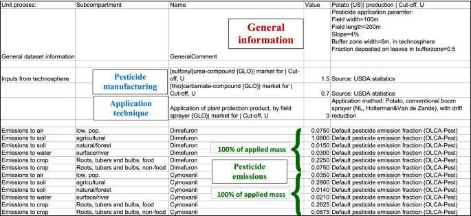
Illustrative example for representing and documenting pesticide application and emission data in crop datasets in LCI databases
-
a.

5.2 Changes needed in LCI databases: food supply chain
In the following, we describe an approach for the modelling of the fate of the active ingredients during later stages in the food supply chain. The initial amount of the pesticide deposited on the crop surface after application should be recorded in the crop dataset. Note that this amount is generally higher than the amount present at harvest, due to processes like degradation or wash-off occurring between the time of pesticide application and crop harvest.
Pesticide residues on food products can also be reduced by further processing or during storage. As these changes take place later in the food supply chain, they should not be modelled in the crop datasets, but in the respective unit process inventories downstream in the food supply chain. Reduction of pesticide residues during processing and storage can be modelled as negative emissions to food, in some cases combined with emissions to non-food or environmental compartments as illustrated in Fig. 9. If degradation occurs e.g., during storage or transport (a), the respective amount is recorded as a negative emission to food. The resulting amount of pesticide and the human toxicity impact will thus be reduced accordingly. In case (b), co-products are generated during processing, which is destined to the feed market. An example is wheat milling, where wheat bran, germs, etc. are produced as by-products, which are typically used as animal feed. In this case, a negative emission to food and a positive emission to non-food of the same amount would be calculated. The third example is washing, which can remove part of the pesticide residues. In this case, a negative emission to food and a positive emission to water of the same size would be recorded. Later treatment of the wastewater in a wastewater treatment plant needs to be modelled in the respective dataset.

Principle of modelling of pesticide residues on food along the food supply chain
5.3 Changes needed in LCIA methods
In order to calculate human toxicity impacts related to pesticide residues on food, six CFs for human toxicity are required for each pesticide active ingredient for the six crop sub-compartments for food use (Table 4) to reflect the impacts on human toxicity through ingestion of pesticide residues on harvested food products. The CFs should relate to the emission to the crop and, therefore will be fully consistent with the emissions to the air, soil, and water compartments. This can be done by the combination of the PestLCI Consensus Model with dynamiCROP as described in Gentil et al. (2020b). For non-food crop sub-compartments, the CFs will be set to zero, which is a simplification in the case of feedstuffs. For the emissions to air, water and soil, the existing USEtox model can be used.
For freshwater ecotoxicity, no specific CFs exist for the crop surface compartment. We propose to use the CFs for agricultural soil as an intermediate solution until more specific CFs are developed. This is an overestimation in many cases, but we consider it as best solution at the time being. If the whole above-ground biomass is harvested and no wash-off and uptake by the crop are taking place, probably most of the active ingredient, which is not degraded before the harvest, is removed from the field. However, in practice, this is seldom the case, and crop residues remain often in the field. We encourage modellers to develop easy-to-use models or rules to define the fraction remaining in the field and the fraction exported by the harvested products. In addition, the development of terrestrial ecotoxicity models including a crop compartment is needed.
5.4 Changes needed in LCA software
The crop compartment with the respective sub-compartments (Table 4) need to be implemented in the LCA software, in order to include the adapted LCI databases and the new CFs.
6 Limitations of the approach and future research needs
6.1 Limitations of the proposed approach
The estimation of emissions fractions in the inventory phase is a strong simplification of real production systems. The initial distribution, proposed as default, is independent of the climate, the soil, the topography of the field, the properties of the active ingredients, and agricultural practices such as soil tillage, irrigation, or drainage. As a consequence, emission-related processes like run-off, leaching, erosion, volatilisation, wash-off, etc. are considered only by generic factors on a continental level in subsequent fate model of USEtox. The proposed approach therefore cannot reflect differences in pedo-climatic conditions or agricultural practices beyond the application technique, the drift reduction, the field width, and the buffer zone. On the other hand, this approach allows for an easy application and is suitable for the implementation in background LCI databases, where a collection of detailed data for each application is not feasible. The only needed information — the crop and the target class of the pesticide — should be available in most LCI databases. The default application scenarios are a simplification, which is however acceptable for most LCA applications. As shown in the sensitivity analysis, the emission fractions react to several parameters related to the situation in the field. However, the largest source of variability and uncertainty stems from the impact assessment, since the ecotoxicity and human toxicity factors have a high uncertainty (Fantke et al. 2018a, b). The users are advised to check, whether the methodology proposed is adequate to reach the goal of their study and to use other models, if needed.
Cover crops cannot be currently considered by the PestLCI Consensus Model, but a method how cover crops can be considered and application in two case studies for tomato and grapevine production is given in Gentil-Sergent et al. (2021a).
Regarding the impact assessment, still CFs for a number of active ingredients are missing. In the OLCA-Pest project, CFs for USEtox for more than hundred active ingredients have been calculated (Fantke et al. 2020). Nevertheless, CFs for certain substances are still lacking. In such cases, users are advised to calculate the missing CFs by the USEtox model, or — where this is not feasible — to use proxies based on the mode of action. Furthermore, potential interactions between different active ingredients cannot currently be assessed; the toxicity impacts are considered as additive, which is in most cases justified where pesticides are not applied simultaneously to the same field. A mixture of active ingredients could in specific cases lead to higher or lower impacts; however, these effects are largely unknown and thus not considered in the presented approach. Toxicity impacts of pesticide degradation metabolites currently cannot be assessed by USEtox. Adjuvants, surfactants, and wetting agents could have effects on the distribution of emissions as well as on the toxicity impacts of pesticides, either directly, because they have a certain level of toxicity for some organisms, or indirectly, through altering the fate or effect of pesticide active ingredients in the formulation.
Finally, microorganisms used as biological pest control agents cannot currently be taken into account, since methods are lacking for their assessment. This also applies to inorganic substances, such as sulphur, as models are missing that can consider the complex reaction kinetics of such substances in the environment (Kirchhübel and Fantke 2019). Microorganisms such as viruses or bacteria can be handled, if they are applied by similar techniques as chemical pesticides (e.g. by spraying or granulates) and CFs are available for the impact assessment.
6.2 Future research needs
The OLCA-Pest project has made a big step forward in the operationalisation of emission modelling and toxicity assessment for pesticides in agri-food LCA. Nevertheless, further research is needed to remedy the weaknesses and gaps in the current methodology. The OLCA-Pest team has identified a number of needs for further research related to the PestLCI Consensus Model.
Further development and testing of the secondary emissions is needed. In particular, care has to be taken to avoid double counting and omissions between the inventory and impact assessment phases, and to ensure a consistent mass balance. This might need a recalculation of CFs. Using secondary emissions would allow a much more specific assessment by better taking into account the effects of soil, climate and agricultural practices in the LCI.
Pesticide application techniques are developing fast. Models should be extended in order to include new application techniques (e.g. sprayers with lower emissions such as adaptive sprayers) and for tropical regions (Gentil-Sergent et al. 2021b). The methods developed for the assessment of production systems with cover crops (Gentil-Sergent et al. 2021a) should be implemented. The pre- and post-treatment phases like preparation of the pesticide slurry, filling of tanks, management of tank bottoms at the end of treatment, and washing/rinsing of equipment should be better integrated into the assessment because they can generate significant contamination of both humans and ecosystems.
Inorganic compounds such as metal-based pesticides or sulphur can be assessed by using the default emission fractions for the initial distribution, but currently cannot be considered in the assessment of the secondary emissions. Metal-based pesticides and active ingredients containing metal ions require the development or adaptation of approaches to be included in emission models (see e.g. Viveros Santos et al. 2018; Owsianiak et al. 2015). Inorganic pesticides require the development of separate emission and characterisation models. Current models are unable to account for the complex reaction kinetics and dynamics of inorganic pesticides and hence need to better account for chemical reaction processes in the different environmental media. Metal emissions from pesticides need to be combined with other sources of metals, such as fertilisers, and be integrated in the overall mass balance of metals.
We identified further several research needs related to the toxicity assessment of pesticides in general. Human impacts of pesticide residues in food crops need to be included systematically in agri-food LCA. Today, dynamiCROP (Fantke et al. 2011a, b) is available for expert practitioners and not included in LCA software. The approach developed by OLCA-Pest proposes a way to include this assessment in a systematic way in mainstream LCA applications, but needs to be further developed. In particular, specific CFs for human toxicity have to be calculated by dynamiCROP, starting from the pesticides deposited on the food crop surface (see Sect. 5.3).
CFs for ecotoxicity need to be developed for the fraction deposited on the crop surface. The fate of pesticides such as volatilisation, wash-off, and degradation as well as the harvested fraction of the biomass should be taken into account.
The exposure of bystanders (Ryberg et al. 2018) and agricultural workers during application and also during pre-post treatment phases require the development or improvement of initial models for characterising exposure and effects of pesticides on human workers and bystanders.
Pollinators and impacts on other ecosystem functional groups require the advancement of initial models to characterise exposure and effects of pesticides on pollinating insects (Crenna et al. 2020), soil organisms, predatory birds, groundwater, and sediment-dwelling organisms need to be newly developed or existing approaches extended and operationalised for a consistent integration into existing LCIA ecotoxicity characterisation.
Metabolites need to be consistently characterised, since various chemical and biological pesticides undergo complex transformation processes. This requires additional data efforts to understand the metabolic fractions, media, and finally physicochemical property and effect data for all metabolites, of which the latter is currently the main limiting aspect.
Accounting for biological pest control technologies (all methods of plant protection using natural mechanisms): organic “natural” compounds, new upcoming application technologies, dissemination and effects of “natural enemies”, etc. Biological pesticides require completely different approaches for characterising emission, fate, exposure, and effect mechanisms. Only based on additional efforts to account for the emission and impact characteristics of each of these biopesticides, it will be possible to ultimately evaluate and compare alternative and chemical pesticide-based farming practices.
7 Conclusions
As mentioned in the introduction, there is a real challenge to improve the consideration of pesticides in agricultural LCA in a consistent way avoiding gaps or overlaps between LCI and LCIA. In addition, the proposed solutions must meet two main expectations that are sometimes difficult to reconcile: (i) LCA for diagnosis and eco-design of agricultural activities (in which pesticides are a major foreground activity) and (ii) LCA of food products life cycle (in which pesticides are a background activity). In this context, the framework proposed in this paper allows to implement the pesticide consensus in LCI databases and LCA software for background applications. It ensures that the mass balance of the pesticide emitted after application is preserved throughout the whole assessment. It allows for a consistent assessment of ecotoxicity and human toxicity, which currently is hindered by inconsistencies between models and databases. This results in a clear and consistent interface between the LCI and LCIA phases. The implementation in LCI databases is possible with the currently available data, which considerably simplifies the procedure. Following the recommendation for the organisation of metadata ensures that the pesticide emissions are transparently documented in crop datasets. A concept is presented to model the removal of pesticide residues on food during further processing, which is consistent with the modelling at crop level and with the general requirements of LCI databases.
We hope that the presented approach will contribute to a systematic and comprehensive inclusion of pesticide emissions and toxicity impact assessment in mainstream LCA applications in the agri-food sector. We encourage LCI database developer, LCA software providers, and LCA practitioners to implement this approach.
Data availability
Data from the OLCA-Pest project are available from https://www.sustainability.man.dtu.dk/english/research/qsa/research/research-projects/olca-pest.
References
Berthoud A, Maupu P, Huet C, Poupart A (2011) Assessing freshwater ecotoxicity of agricultural products in life cycle assessment (LCA): a case study of wheat using French agricultural practices databases and USEtox model. Int J LCA 16(8):841–847
Birkved M, Hauschild MZ (2006) PestLCI - a model for estimating field emissions of pesticides in agricultural LCA. Ecol Model 198:433–451
Crenna E, Jolliet O, Collina E, Sala S, Fantke P (2020) Characterising honey bee exposure and effects from pesticides for chemical prioritisation and life cycle assessment. Environ Int 138:105642. https://doi.org/10.1016/j.envint.2020.105642
Dijkman TJ, Birkved M, Hauschild MZ (2012) PestLCI 2.0: a second generation model for estimating emissions of pesticides from arable land in LCA. Int J LCA 17:973–986
European Commission (2019) Product Environmental Footprint Category Rules Guidance, Version 6.3 – May 2018, 238p. https://eplca.jrc.ec.europa.eu/permalink/PEFCR_guidance_v6.3-2.pdf
Fantin V, Righi S, Buscaroli A, Garavini G, Zamagni A, Dijkman T, Bonoli A (2016) Application of PestLCI model to site-specific soil and climate conditions: the case of maize production in Northern Italy. In: Proceedings of X Conference of Italian LCA Network Association, Ravenna, 23–24
Fantke P, Jolliet O (2016) Life cycle human health impacts of 875 pesticides. Int J LCA 21:722–733
Fantke P (2019) Modelling the environmental impacts of pesticides in agriculture. In: Weidema BP (ed) Assessing the Environmental Impact of Agriculture. Burleigh Dodds Science Publishing, Cambridge, United Kingdom, pp 177–228
Fantke P, Antón A, Grant T, Hayashi K (2017) Pesticide emission quantification for life cycle assessment: a global consensus building process. J LCA Japan 13:245–251
Fantke P, Aylward L, Bare J, Chiu WA, Dodson R, Dwyer R, Ernstoff A, Howard B, Jantunen M, Jolliet O, Judson R (2018a) Advancements in life cycle human exposure and toxicity characterization. Environ Health Perspect 126(12):125001
Fantke P, Aurisano N, Bare J, Backhaus T, Bulle C, Chapman PM, De Zwart D, Dwyer R, Ernstoff A, Golsteijn L, Holmquist H, Jolliet O, McKone TE, Owsianiak M, Peijnenburg W, Posthuma L, Roos S, Saouter E, Schowanek D, van Straalen NM, Vijver MG, Hauschild M (2018b) Toward harmonizing ecotoxicity characterization in life cycle impact assessment. Environ Toxicol Chem 37:2955–2971
Fantke P, Charles R, de Alencastro LF, Friedrich R, Jolliet O (2011a) Plant uptake of pesticides and human health: Dynamic modeling of residues in wheat and ingestion intake. Chemosphere 85:1639–1647
Fantke P, Chiu WA, Aylward L, Judson R, Huang L, Jang S, Gouin T, Rhomberg L, Aurisano N, McKone T, Jolliet O (2021) Exposure and toxicity characterization of chemical emissions and chemicals in products: global recommendations and implementation in USEtox. Int J LCA 26(5):899–915
Fantke P, Juraske R, Antón A, Friedrich R, Jolliet O (2011b) Dynamic multicrop model to characterise impacts of pesticides in food. Environ Sci Technol 45:8842–8849
Fantke P, Wieland P, Juraske R, Shaddick G, Itoiz ES, Friedrich R, Jolliet O (2012) Parameterisation models for pesticide exposure via crop consumption. Environ Sci Technol 46(23):12864–12872
Fantke P, Antón A, Basset-Mens C, Nemecek T, Roux P, Renaud-Gentié C, Naviaux P, Gentil C, Peña N, Melero C (2020) OLCA-Pest – Final Project Report, 12p. https://www.sustainability.man.dtu.dk/english/-/media/centre/qsa/olca-pest/deliverables/olca-pest_finalreport_public.pdf
Gentil C, Basset-Mens C, Manteaux S, Mottes C, Maillard E, Biard Y, Fantke P (2020a) Coupling pesticide emission and toxicity characterisation models for LCA: application to open-field tomato production in Martinique. J Clean Prod 277:124099
Gentil C, Fantke P, Mottes C, Basset-Mens C (2020b) Challenges and ways forward in pesticide emission and toxicity characterization modeling for tropical conditions. The Int J LCA 25(7):1290–1306
Gentil-Sergent C, Basset-Mens C, Gaab J, Mottes C, Melero C, Fantke P (2021a) Quantifying pesticide emission fractions for tropical conditions. Chemosphere 275:130014. https://doi.org/10.1016/j.chemosphere.2021.130014
Gentil-Sergent C, Basset-Mens C, Renaud-Gentié C, Mottes C, Melero C, Launay A, Fantke P (2021b) Introducing ground cover management in pesticide emission modeling. Integr Environ Assess Manage. https://doi.org/10.1021/acs.jafc.1c00151
Gutsche V, Rossberg D (1997) Synops 1.1: a model to assess and to compare the environmental risk potential of active ingredients in plant protection products. Agric Ecosyst Environ 64:181–188
Kirchhübel N, Fantke P (2019) Getting the chemicals right: toward characterizing toxicity and ecotoxicity impacts of inorganic substances. J Clean Prod 227:554–565
Margni M, Rossier D, Crettaz P, Jolliet O (2002) Life cycle impact assessment of pesticides on human health and ecosystems. Agric Ecosyst Environ 93(1–3):379–392
Melero C, Gentil C, Peña N, Renaud-Gentié C, Fantke P (2020a) Documentation of air, soil, and water emission modelling in PestLCI Consensus model. OLCA-Pest deliverable 3.3. https://www.sustainability.man.dtu.dk/english/-/media/centre/qsa/olca-pest/deliverables/olca-pest_d3-3_public.pdf
Melero C, Nemecek T, Fantke P (2020b) Web based system, documentation, user guide for organic and inorganic pesticides. OLCA-Pest deliverable 5.1. https://www.sustainability.man.dtu.dk/english/-/media/centre/qsa/olca-pest/deliverables/olca-pest_d5-1_public.pdf
Nemecek T, Bengoa X, Lansche J, Mouron P, Riedener E, Rossi V, Humbert S (2015) World Food LCA Database: methodological guidelines for the life cycle inventory of agricultural products. Version 3.0. Lausanne and Zurich
Neto B, Dias AC, Machado M (2013) Life cycle assessment of the supply chain of a Portuguese wine: From viticulture to distribution. Int J LCA 18:590–602
Nordborg M, Cederberg C, Berndes G (2014) Modeling potential freshwater ecotoxicity impacts due to pesticide use in biofuel feedstock production: the cases of maize, rapeseed, salix, soybean, sugar cane, and wheat. Environ Sci Technol 48(19):11379–11388
Owsianiak M, Holm PE, Fantke P, Christiansen KS, Borggaard OK, Hauschild MZ (2015) Assessing comparative terrestrial ecotoxicity of Cd Co, Cu, Ni, Pb, and Zn: The influence of aging and emission source. Environ Pollut 206:400–410. https://doi.org/10.1016/j.envpol.2015.07.025
Peña N, Anton A, Melero C, Gentil C, Nemecek T, Fantke P (2020) Definition of a consistent set of archetypes for climate, soil, crop, pesticide, and application method combinations for use in LCA. OLCA-Pest Deliverable 5:3
Poore J, Nemecek T (2018) Reducing food’s environmental impacts through producers and consumers. Science 360:987–998
Potting J, Hauschild M (2006) Spatial differentiation in life cycle impact assessment: a decade of method development to increase the environmental realism of LCIA. Int J LCA 11:11–13
Renaud-Gentié C, Dijkman TJ, Bjørn A, Birkved M (2015) Pesticide emission modelling and freshwater ecotoxicity assessment for Grapevine LCA: adaptation of PestLCI 2.0 to viticulture. Int J LCA 20(11):1528–1543
Rosenbaum R, Anton A, Bengoa X, Bjørn A, Brain R, Bulle C, Cosme N, Dijkman T, Fantke P, Felix M, Geoghegan T, Gottesbüren B, Hammer C, Humbert S, Jolliet O, Juraske R, Lewis F, Maxime D, Nemecek T, Payet J, Räsänen K, Roux P, Schau E, Sourisseau S, van Zelm R, von Streit B, Wallman M (2015) The Glasgow consensus on the delineation between pesticide emission inventory and impact assessment for LCA. Int J LCA 20:765–776
Rosenbaum RK, Bachmann TM, Gold LS, Huijbregts MAJ, Jolliet O, Juraske R, Koehler A, Larsen HF, MacLeod M, Margni M, McKone TE, Payet J, Schuhmacher M, van de Meent D, Hauschild MZ (2008) USEtox-the UNEP-SETAC toxicity model: recommended characterisation factors for human toxicity and freshwater ecotoxicity in life cycle impact assessment. Int J LCA 13:532–546
Ryberg MW, Mosqueron RRK, L, Fantke P (2018) Addressing bystander exposure to agricultural pesticides in life cycle impact assessment. Chemosphere 197:541–549. https://doi.org/10.1016/j.chemosphere.2018.01.088
van Zelm R, Larrey-Lassalle P, Roux P (2014) Bridging the gap between life cycle inventory and impact assessment for toxicological assessments of pesticides used in crop production. Chemosphere 100:175–181. https://doi.org/10.1016/j.chemosphere.2013.11.037
Vázquez-Rowe I, Villanueva-Rey P, Iribarren D, Teresa Moreira M, Feijoo G (2012) Joint life cycle assessment and data envelopment analysis of grape production for vinification in the Rías Baixas appellation (NW Spain). J Clean Prod 27:92–102. https://doi.org/10.1016/j.jclepro.2011.12.039
Viveros Santos I, Bulle C, Levasseur A, Deschênes L (2018) Regionalised terrestrial ecotoxicity assessment of copper-based fungicides applied in viticulture. Sustainability 10:2522. https://doi.org/10.3390/su10072522
Wannaz C, Fantke P, Jolliet O (2018a) Multi-scale spatial modeling of human exposure from local sources to global intake. Environ Sci Technol 52:701–711
Wannaz C, Fantke P, Lane J, Jolliet O (2018b) Source-to-exposure assessment with the Pangea multi-scale framework - case study in Australia. Environ Sci-Proc Imp 20:133–144
Wannaz C, Franco A, Kilgallon J, Hodges J, Jolliet O (2018c) A global framework to model spatial ecosystems exposure to home and personal care chemicals in Asia. Sci Total Environ 622–623:410–420
Wernet G, Bauer C, Steubing B, Reinhard J, Moreno-Ruiz E, Weidema B (2016) The ecoinvent database version 3 (part I): overview and methodology. Int J LCA 21(9):1218–1230
Westh TB, Hauschild MZ, Birkved M, Jørgensen MS, Rosenbaum RK, Fantke P (2015) The USEtox story: a survey of model developer visions and user requirements. Int J LCA 20:299–310
Funding
Open access funding provided by Agroscope. This work was financially supported by the OLCA-Pest project funded by the French Environment and Energy Management Agency, ADEME (GA no. 17–03-C0025).
Author information
Authors and Affiliations
Corresponding authors
Ethics declarations
Conflict of interest
The authors declare no competing interests.
Additional information
Communicated by Brad G. Ridoutt.
Publisher's Note
Springer Nature remains neutral with regard to jurisdictional claims in published maps and institutional affiliations.
Supplementary information
Below is the link to the electronic supplementary material.
Rights and permissions
Open Access This article is licensed under a Creative Commons Attribution 4.0 International License, which permits use, sharing, adaptation, distribution and reproduction in any medium or format, as long as you give appropriate credit to the original author(s) and the source, provide a link to the Creative Commons licence, and indicate if changes were made. The images or other third party material in this article are included in the article's Creative Commons licence, unless indicated otherwise in a credit line to the material. If material is not included in the article's Creative Commons licence and your intended use is not permitted by statutory regulation or exceeds the permitted use, you will need to obtain permission directly from the copyright holder. To view a copy of this licence, visit http://creativecommons.org/licenses/by/4.0/.
About this article

Cite this article
Nemecek, T., Antón, A., Basset-Mens, C. et al. Operationalising emission and toxicity modelling of pesticides in LCA: the OLCA-Pest project contribution. Int J Life Cycle Assess 27, 527–542 (2022). https://doi.org/10.1007/s11367-022-02048-7
Received:
Accepted:
Published:
Issue Date:
DOI: https://doi.org/10.1007/s11367-022-02048-7