
Abstract
Discrete time Markov decision process is studied and the minimum reward risk model is established for the reservoir long-term generation optimization. Different form the commonly used optimization criterion of best expected reward in reservoir scheduling, the probability that the expected generation of the whole period not exceeding the predete reward target to be smallest is chosen as the optimizing target for this random process. For the hydropower tends to operate as peak-clipping mode in Market-based model to gain more profits, the function of electricity price and output can be founded by analyzing on the typical day load course of the electricity system. Compared with the generally used criteria of the largest expectation power generation model, this model is fitted for the decision-making in which the risk is needed to be limited to reflect the risk preference of the policy makers. Stochastic dynamic programming method is adopted to solve the model and the model is tested on the Three Gorges Hydropower Station.
Because of the uncertainty of the inflow runoff, reservoir operation is a random process. Best expected reward is a commonly used optimization criterion in reservoir scheduling, related literatures see (Zhang 1987; Wang et al. 2002b, 2014; Zhang et al. 2006, 2007; Chang et al. 2005; Ahmad et al. 2014). However, this criterion is insensitive on risk, a strategy maximizing the random variable of expected reward may cause it to get a lower value on an unacceptable probability. The criterion is not appropriate to optimization problems which need some directly reflection or restriction of risks. For the scheduling optimization of hydropower station, in order to guaranteeing a certain level of hydropower reward, the scheduling strategy should make the total annual expected hydropower reward as large as possible, meanwhile, it demands the probability that the actual reward lower than a predetermined value should not be greater than a given level. Thus, only taking the expected reward as optimization target is not enough, other optimization criterion is necessary to be chosen to reflect risk of the practical problems and satisfy the decision maker’s will or risk appetite.
This paper presents a minimum reward risk model in reservoir optimization scheduling. According to this model, risk probability is employed as the optimization target to seek for the optimum scheduling strategy. The specific principle of this model can be described as: for the predetermined level of total hydropower profit during scheduling period, the optimum control strategy of reservoir scheduling is seek to minimize the risk probability that the expected generation reward lower than the predetermined value. With the help of this model, the decision makers can select different control policies according to their risk tolerance and preference freely.
1 Markov Decision Process
This paper focus on the study of discrete-time, non-time-homogeneous Markov decision model (Liu 2004), which has the following structure:
where S t is the system state set within period t; \( {A}_t={\displaystyle {\cup}_{i\in {S}_t}{A}_t}(i) \) is the action set. For some state i ∈ S t , a set A t (i) of allowable actions during the t period can be taken; p t = {p a ij , i ∈ S t , j ∈ S t + 1, a ∈ A t (i)} is a system state situation transition probability matrix which satisfies \( {\displaystyle \sum_{j\in {S}_{t+1}}{p}_{ij}^a}=1 \); Function R t = {R t (⋅|i, a, j)} is adopt as the reward distribution and satisfying R([M 1, M 2]|i, a, j) = 1, where constants M 1, M 2 denote the upper and lower bound of reward respectively.
Model (1) describes a stochastic decision making process at each discrete time t = 0,......, T. Variables i t , a t , b t mean the system state, action-taken and period reward at time t respectively. System operation can be described as follows: supposing the system is in state i t = i at time t, taking an action a t = a ∈ A t (i), then:
-
(1)
the system transfers to the next state i t + 1 = j with probability p a ij , which meaning Pr ob(i t + 1 = j|i t = i, a t = a) = p a ij ;
-
(2)
Obtain the period reward r t , which is a random variable obeying R(⋅|i, a, j) probability distribution.
Once the system transferred to a new State, it will take new actions and thus developing continuously.
π = {a t , t = 1 … T} is defined as a control sequence composed of action set which satisfy a t ∈ A t (i), t = 1.... T. A Markov decision process is determined by a special action sequence π and the initial state i 1 = i. r t (i, a, j) is called the reward function for replacing the R t (⋅|i, a, j) if R t (⋅|i, a, j); i ∈ S t , j ∈ S t + 1, a ∈ A t (i) follows degenerating distribution and meets R t ({r t (i, a, j)}|i, a, j) = 1. r t (i, a, j) is the function of i, a, j.
2 Minimum Reward Risk Model based on Markov Decision Process
Taking variable \( {B}_T^{\pi }={\displaystyle \sum_{t=1}^T{r}_t} \) as the total expected reward produced by applying strategy π.
2.1 Minimum Risk Model
For a given case including constants of predetermined reward x, the number of T stages and the initial state i 1 of the system, decision control target is to achieve minimal risk probability that the total expected reward lower than the predetermined reward at the end of stage T. Let π ∈ ∏ and seeking policy π* as:
Where i t , x t , a t , e t = (i t , x t ), r t are system state, target reward value, action-taken, decision state and the obtained stage reward respective. π* is the optimal scheduling strategy, Π is a set of decision sequences which are called decision sequence space.
2.2 Objective Function and Optimal Value Function
Taking formula
as the objective function resulted by the strategy π where E is the decision state set. Thus, the formula
is the optimal value function of the minimum risk model. Supposing a control sequence π* ∈ Π subject to \( {F}_T^{\pi^{*}}\left(i,x\right)={F}_T^{*}\left(i,x\right),\begin{array}{cc}\hfill \hfill & \hfill \forall \left(i,x\right)\in E\hfill \end{array} \), π* is the optimal scheduling strategy during stage T.
3 Solution Algorithm of Minimum Risk Model
Supposing the finite set W = {r 1, r 2, r 3......., r m }, r 1 < r 2 < … < r m satisfies R t (W|i, a, j) = 1, \( i\in {S}_t,j\in {S}_{t+1},a\in {A}_t(i),\begin{array}{cc}\hfill \hfill & \hfill t=1.....T\hfill \end{array} \), let p a ijr = p a ij R t ({r}|i, a, j). Inverse timing recursive algorithm is adopted to solve the model.
3.1 Dynamic Recursive Equation of Remaining Profit Risk Function
Taking
as the dynamic recursive equation of remaining profit risk function with boundary condition:
Let I [0,+ ∞](x) be the characteristic function of set [0, + ∞], which means
Denoting:
where b t (i, x, a) denotes the system probability that the total reward lower than x in stage t from current to the end of scheduling period, when system is in state i for target x, taking action a. I t (i, x) is the minimum expected probability taking the optimal action in period t.
3.2 Inverse Time Sequence Recursion Process
Based on the stochastic dynamic programming principle, the recursive optimization process include following three steps complying with Inverse time sequence (Askew 1974).
-
Step 1
This step is for the last period of decision-making.
The relevant variable values can be calculated by the following formula
$$ {b}_{T-1}\left(i,{r}_k,a\right)={\displaystyle \sum_{j\in {S}_T}{\displaystyle \sum_{r\le {r}_K}{p}_{ijr}^a}}\begin{array}{ccc}\hfill, \hfill & \hfill \hfill & \hfill \hfill \end{array}\begin{array}{cc}\hfill \hfill & \hfill i\in {S}_{T-1}\hfill \end{array},a\in {A}_{T-1}(i) $$(9)$$ {I}_{T-1}\left(i,{r}_k\right)=\underset{a\in {A}_{T-1}(i)}{ \min}\left\{{b}_{T-1}\left(i,{r}_k,a\right)\right\},\begin{array}{cc}\hfill \hfill & \hfill i\in {S}_{T-1}\hfill \end{array} $$(10)$$ {A}_{T-1}^{*}\left(i,{r}_k\right)=\left\{a\left|a\in {A}_{T-1}(i),\right.\begin{array}{cc}\hfill \hfill & \hfill {b}_{T-1}\hfill \end{array}\left(i,{r}_k,a\right)={I}_{T-1}\left(i,{r}_k\right)\right\} $$(11)For the formula (11), which means that there perhaps to be more than on decisions can achieve the same minimum risk value. One of them is enough of course. Here variable g T − 1(i, r k ) is used as the optimal decision action for the last period.
$$ {g}_{T-1}\left(i,{r}_k\right)\in {A}_{T-1}^{*}\left(i,{r}_k\right),k=1,2......m-1;\begin{array}{cc}\hfill \hfill & \hfill {g}_{T-1}\left(i,{r}_m\right)\hfill \end{array}\in {A}_{T-1}(i) $$(12)Variable r means the current period generating profit, which is divided into m score ascending.
Second, during the actual scheduling decision-making time for the predetermined generation profit x and system state i, following formula can be adopted to decide the optimal decision action and its corresponding minimum risk probability.
$$ {F}_{T-1}^{*}\left(i,x\right)=\left\{\begin{array}{l}0,\begin{array}{cccc}\hfill \hfill & \hfill \hfill & \hfill \hfill & \hfill \begin{array}{cc}\hfill \hfill & \hfill x<{r}_1,\hfill \end{array}\hfill \end{array}\\ {}{I}_{T-1}\left(i,{r}_k\right),\begin{array}{cc}\hfill \hfill & \hfill {r}_k\le x<{r}_{k+1},k=1\dots m-1\hfill \end{array}\\ {}1\begin{array}{cccc}\hfill \hfill & \hfill \hfill & \hfill \hfill & \hfill \begin{array}{cc}\hfill \hfill & \hfill x\ge {r}_m\hfill \end{array}\hfill \end{array}\end{array}\right. $$(13)$$ {A}_{T-1}^{*}\left(i,x\right)=\left\{\begin{array}{l}{A}_{T-1}(i)\begin{array}{cc}\hfill \begin{array}{cc}\hfill \hfill & \hfill \hfill \end{array}\hfill & \hfill x<{r}_1,x\ge {r}_m\hfill \end{array}\\ {}{A}_{T-1}^{*}\left(i,{r}_k\right)\begin{array}{cc}\hfill \hfill & \hfill {r}_k\le x<{r}_{k+1},k=1\dots m-1\hfill \end{array}\end{array}\right. $$(14)$$ {g}_{T-1}\left(i,x\right)=\left\{\begin{array}{l}{g}_{T-1}\left(i,{r}_m\right),\begin{array}{ccc}\hfill \hfill & \hfill x<{r}_1\begin{array}{cc}\hfill \hfill & \hfill or\hfill \end{array}\hfill & \hfill x\ge {r}_m\hfill \end{array}\\ {}{g}_{T-1}\left(i,{r}_k\right),\begin{array}{cc}\hfill \hfill & \hfill {x}_k\le x<{r}_{k+1},k=1....m-1.\hfill \end{array}\end{array}\right. $$(15) -
Step 2
Supposing F * t (i, x)(∀ i ∈ S t )、 A * t 、 g t have been obtained for some period t. The predetermined generation profit variable X from current t period to the scheduling end is divided into M score as x 1 < x 2 < … < x M . Following is the special recursive calculation method to achieve the optimal scheduling action and the corresponding minimum risk probability for period t − 1.
Form period t − 1 to the scheduling end, the predetermined generation profit variable can be expressed as x k + r h , where k = 1, 2....., M, h = 1, 2...., m. Variable U can be taken as this predetermined generation profit. Hence for any transferring state j form period t − 1 to t,
$$ j\in {S}_t,r\in W,\kern1em {F}_t^{*}\left(j,x-r\right)=\left\{\begin{array}{l}0\begin{array}{cccc}\hfill \hfill & \hfill \hfill & \hfill \hfill & \hfill \begin{array}{cc}\hfill \hfill & \hfill x<{u}_1\hfill \end{array}\hfill \end{array}\\ {}{F}_t^{*}\left(j,{u}_k-r\right)\begin{array}{cc}\hfill \hfill & \hfill {u}_k\le x<{u}_{k+1},1\le k<N\hfill \end{array}\\ {}1\begin{array}{cccc}\hfill \begin{array}{cc}\hfill \hfill & \hfill \hfill \end{array}\hfill & \hfill \hfill & \hfill \hfill & \hfill x\ge {u}_N\hfill \end{array}\end{array}\right. $$(16)Then, the special optimal scheduling action and the corresponding minimum risk probability for period t − 1 can be calculate as:
$$ {b}_{t-1}\left(i,{u}_k,a\right)={\displaystyle \sum_{j\in {S}_t}{\displaystyle \sum_{r\in W}{p}_{ijr}^a}}{F}_t^{*}\left(j,{u}_k-r\right),i\in {S}_{t-1},a\in {A}_{t-1}(i) $$(17)$$ {I}_{t-1}\left(i,{u}_k\right)=\underset{a\in {A}_{t-1}(i)}{ \min}\left\{{b}_{t-1}\left(i,{u}_k,a\right)\right\},i\in {S}_{t-1} $$(18)$$ {A}_{t-1}^{*}\left(i,{u}_k\right)=\left\{\left.a\right|a\in {A}_{t-1}(i),{b}_{t-1}\left(i,{u}_k,a\right)={I}_{t-1}\left(i,{u}_k\right)\right\},\begin{array}{cc}\hfill \hfill & \hfill i\in {S}_{t-1}\hfill \end{array} $$(19)Choose g t − 1(i, u k ) ∈ A * t − 1 (i, u k ), k = 1,......, N − 1, g t − 1(i, u N ) ∈ A t − 1(i) as the t − 1 period optimal scheduling action.
As similar as the step 1, for a given predetermined generation profit x and system state i, the corresponding optimization decision for period t − 1 can be achieve as follows:
$$ {F}_{t-1}^{*}\left(i,x\right)=\left\{\begin{array}{l}0\begin{array}{cccc}\hfill \hfill & \hfill \hfill & \hfill \begin{array}{cc}\hfill \hfill & \hfill \hfill \end{array}\hfill & \hfill x<{u}_1\hfill \end{array}\\ {}{I}_{t-1}\left(i,{u}_k\right),\begin{array}{cc}\hfill \hfill & \hfill {u}_k\le x<{u}_{k+1},k=1,....N-1,\hfill \end{array}\\ {}1\begin{array}{cccc}\hfill \hfill & \hfill \hfill & \hfill \hfill & \hfill \begin{array}{cc}\hfill \hfill & \hfill x\ge {u}_N\hfill \end{array}\hfill \end{array}\end{array}\right. $$(20) (21)
(21) (22)
(22) -
Step 3
If t − 1 > 0, replacing t by t − 1 in step 2 and return to step 2. If t − 1 = 0, the iteration stop. From the steps above, the optimal value function F *0 and the best policy π* = {g 0, g 1,.... g T ) can be calculated for the whole scheduling period T.


4 Application of Minimum Risk Model in Hydropower Optimal Scheduling
For the reservoir mid-long term optimized operation system, the whole scheduling period is often 1 year and is divided into several periods by a month or 10 days, related literatures see (Wang et al. 2002b; Huang and Wu 1993; Jahandideh-Tehrani and Bozorg Haddad 2015; Liu et al. 2006; Xie et al. 2012) The reservoir storage level and period of runoff composed of the system state variables (Z t , Q t ), t = 0,.... T. Variable X is the predetermined generation profit and (Z t , Q t , X) being the decision state. Reservoir outflow U t is the decision variable. The period generation reward r t is the product of generation output N t and electricity price p t , r t = p t N t . In this study, period electricity price r t is assumed as a function of output N t , \( {p}_t={p}_t\left({N}_t\right),\begin{array}{cc}\hfill \hfill & \hfill t=0,....N\hfill \end{array} \).
Usually, to obtain greater generation benefit, the hydropower tends to peak cutting operate basis on electricity market mode. Therefore, the relationship between N t and p t can be determined by analyzing of the typical daily load curve of the power system.
4.1 Mathematical Model
-
①
Dynamic recursive equation of remaining profit risk function
$$ {F}_t^{*}\left(i,x\right)=\underset{u_t}{ \min}\left\{{\displaystyle \sum_{j\in {S}_{t+1},r\in W}{p}_{ijr}^{u_t}}{F}_{t+1}^{*}\left(j,x-{r}_t\right)\right\}\kern0.75em i\in {S}_t=\left({Z}_t\times {Q}_t\right) $$(23)With boundary condition: F * T (i, x) = I [0,+ ∞](x).
r t (z t , q t , u t ) is the generating profit function of the t scheduling period, which depends on the factors of actual output, penalty terms and the electricity price, r t = p t × (N t + min{0, α(N t − N f )}). N f is the firm power and α the penalty coefficient, which can be calculated by using of iterative trial method to meet the requirement of given guarantee rate (Wang et al. 2002b).
-
②
Constraint condition:
-
a.
State transition equation of water storage: V t + 1 = V t + (Q t − U t )Δt;
-
b.
Outflow process constraint: \( {U}_t\le {U}_t\le {\overline{U}}_t \);
-
c.
Reservoir storage process constraint: \( {\overline{V}}_{death}\le {V}_t\le {\overline{V}}_t \)
-
d.
Guarantee rate constraint: p(N t > N f ) ≥ p f
-
a.
-
③
Function of period reward price and generation output
Under the mode of power market-based, price, discharge and water head are three variable factors influencing the operation of hydropower plant. Generator capacity price related to its operating position in the system load chart: peak load electricity price is the highest while valley load price lowest. Due to hydropower’s premium performance of peak regulation and frequency modulation, the hydropower tends to peak cutting operate to get greater profit in actual operation. With increasing in work hours, the average electricity price is reduced as hydropower operating position moves down in the system load chart. Therefore, based on the reasonable assumption that hydropower tends to peak cutting operate, how to determine the functional relationship between hydropower duration and average price is the key of establishing the functional relationship of average period price and the output.
This paper analyzes typical daily load process of power system for each period to determine the functional relationship p = p(t) of average electricity price p and work duration t, which consists of the following steps. Although this paper study mid-long term optimized operation system for hydropower stations and the period is month, the special daily running is supposed as following peak cutting operation principle. That is to say: power demand in peak load period should always be met first whenever in dry seasons or wet seasons; and if water quantity is rich, operating position may move down to base load on condition of target of the maximum hydropower profit.
-
a.
Select typical daily load curve of the power system during each scheduling period t, the values between the minimum and maximum of the load curve are discretized from high to low. once the curve according to duration time has been drawn again, the curve of load P and duration t is obtained, as show in Fig. 1;
Fig. 1 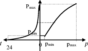
Curve of output-price and curve of load-cumulative duration
-
b.
Suppose the maximum load price p max and the minimum load price p min. Make linear interpolation due to load sizes and get corresponding price dp i at every discrete load points dP i ;
-
c.
When \( \frac{{\displaystyle \sum d{P}_id{p}_i\varDelta t}}{{\displaystyle \sum d{P}_i\varDelta t}}=\overset{-}{p_t} \), the iteration stops; where \( {\overline{p}}_t \) is the average electricity price in period t based on historical price data;
-
d.
According to the determined value p max、 p min and make linear interpolation due to the load size, determine relationship curve of load P and price p(P), as described in Fig. 1;
-
e.
According to Fig. 1, draw relationship curve p(t) ~ t of duration and price, as shown in Fig. 2.
Fig. 2 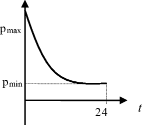
Curve of price-cumulative duration
Supposing average output of hydropower plant of current period is Nt and the capacity of hydropower plant is N0, the daily minimum work hours are t = Nt/N0 . The average electricity price corresponding to output N t can be calculated through interpolation of the curve p(t) ~ t.
-
a.
-
④
Convergence Condition
Inverse timing recursion begin from Tth period at the end of the hydrological cycle until to the 0th beginning period . The first loop is completed, which can be expressed as F (1) T → F (1)0 , let F (2) T = F (1)0 ; then continue the second loop F (2) T → F (2)0 and the kth loop F (k) T → F (k)0 in sequence. Under the appropriate condition, \( \underset{k\to \infty }{ \lim}\left({F}_0^{(k)}-{F}_T^{(k)}\right)= const \) will appear and the stable policy is gained. Then the loop stops (Wang et al. 2002a).
In figures above, where the unit of variable t is hour, output P is WM, price p is Yuan/WM。


5 Case Application
The China’s three gorges hydropower station is selected as a case study, the minimum reward risk model in mid-long term optimized operation system is proposed. Because mature electricity markets have not been established in china, the price data of market is not available. But author considers a reasonable estimation that the electricity price can be obtained by analyzing the actual operation of the power system and hydropower plant. For three gorges hydropower plant, we assume its average period price is 0.25 Yuan/KW.h. As supplement and perfection to the original model, the optimal target changes into the maximum electricity reward when the given risk of electricity reward is 0 or 1.
Discrete the state variables: both the discrete number of reservoir storage level and runoff are 10, the expected value of generation has a descending discretization number of \( 10\times \left(12-t\right)\begin{array}{cc}\hfill \hfill & \hfill t=0,\ldots 11\hfill \end{array} \). Points of the first scheduling period is 120 with range [0,12P] and points in the last period is 10 with range [0, P]. P denotes total capacity of the three gorges hydropower station, P = 18,200 MW.
Through correlation regression analysis of the historical measured runoff data, we establish seasonal AR(1)model which accord with Markov process. Transition matrix of runoff conditional probability is calculated by massive simulated series. Due to space limitation, detailed description has not been put here.
Through inverse timing iterative calculation and for each discrete decision points (Z t , Q t , X t ), the statistical parameters of release policy during optimal period, expected generation reward and expected guarantee rate and so on is determined by applying of the minimum reward risk model while the model converges.
For a special decision state in current period given as e t = (z, q, x) t , scheduling policy in current state can be adopted by interpolation according to generated policies with discrete decision state. Decision state is three dimensional vector, therefore it belongs to 3D-interpolation. The steps are as follows:
-
① Determine position of decision states, where z i ≤ z < z i + 1, q j ≤ q < q j + 1, x k ≤ x < x k + 1;
-
② Fixed z、 q, x is calculated by using linear interpolation:
According to the optimal risk values corresponding to (z i , q j , x k ) and (z i , q j , x k + 1), risk value of (z i , q j , x) can be determined by interpolating; in the same way, the optimal risk values of the following discrete state points (z i , q j + 1, x), (z i + 1, q j , x), (z i + 1, q j , x), (z i + 1, q j , x) can be determined successively.
-
③ Fixed z, x, q is determined by using linear interpolation:
According to risk values corresponding to generated discrete state points (z i , q j , x) and (z i , q j + 1, x), the risk value corresponding to (z i , q, x) can be obtained by interpolating; so the risk value corresponding to (z i + 1, q, x) can be calculated;
-
④Fixed q、 x, z is determined by using linear interpolation:
According to risk values corresponding to generated points (z i , q, x) and (z i + 1, q, x), the risk value corresponding to (z, q, x) can be determined.
For the Three Gorges Hydropower Station, part of the calculation results statistically as shown in Table 1 when scheduling period starts from early June with the first period water level 145 m and discharge 12,656 m3/s.
Table 1 Statistical table of part of the calculation results
6 Conclusions
Different from the conventional power generation optimization criterion of best expected reward, a minimum decision risk model is developed to generate reservoir scheduling plan, which is the most significant innovation in reservoir scheduling. Event risk probability is put to be the optimal target and optimal control strategy is sought by stochastic dynamic programming method. With the advantage of this model, decision makers have the chance to select different control policies according to their risk tolerance and preference.
Under market mode, this scheduling model is more appropriate to operators and management staff of hydropower station who can make scheduling policy to reflecting their own risk preference according to actual anti-risk abilities of company finance and of reservoir characteristics and so on. Generally speaking, companies with abundant capital power and reservoirs possess good regulation performance have strong ability to resist risk and tend to select the scheduling policies of high income with high risks, vice versa. This will increase the decision flexibility for decision to make the operation of hydropower stations closer to their companies’ reality.
References
Ahmad A, El-Shafie A, Razali SFM, Mohamad ZS (2014) Reservoir optimization in water resources: a review. Water Resour Manag 28:3391–3405. doi:10.1007/s11269-014-0700-5
Askew AJ (1974) Chance constrained dynamic programming and the optimization of water resources systems [J]. Water Resour Res 20:1099–1106
Chang JX, Huang Q, Wang YM (2005) Genetic algorithms for optimal reservoir dispatching. Water Resour Manag 19:321–331. doi:10.1007/s11269-005-3018-5
Huang WC, Wu CM (1993) Diagnostic checking in stochastic dynamic programming[J]. Water Resour Plan Manag ASCE 119(4):490–494
Jahandideh-Tehrani M, Bozorg Haddad O (2015) Hydropower reservoir management under climate change: the karoon reservoir system. Water Resour Manag 29:749–770. doi:10.1007/s11269-014-0840-7
Liu K (2004) Practical Markov decision processes [M]. Tsinghua University Press, Beijing(in Chinese)
Liu B, Chen HP, Zhang GY, Xu SJ (2006) A grid-based system for the multi-reservoir optimal scheduling in huaihe river basin. Lect Notes Comput Sci 3842:672–677
Wang J, Yuan X, Zhang Y (2002a) Application of stochastic dynamic programming in long-term generation operation for three gorges cascade [J]. Power Autom Equip 22(8):54–56, (in Chinese)
Wang J, Shi Q, Wu Y et al (2002b) Long-term optimal generation scheduling model of hydroelectric system and its solution [J]. Power Syst Autom 26(24):22–30, (in Chinese)
Wang XM, Zhou JZ, Shuo OY, Li CL (2014) Research on joint impoundment dispatching model for cascade reservoir. Water Resour Manag 28:5527–5542. doi:10.1007/s11269-014-0820-y
Xie WW, Li BJ, Wang S, Zhang WJ, Fan LZ (2012) Status and prospect of Chinese reservoir scheduling management. Water Resour Power 30(9):59–62
Zhang Y (1987) Optimal management of hydropower [M]. Huazhong University of science and Technology Press, Wuhan(in Chinese)
Zhang M, Ding Y, Yuan X, Li C (2006) Study of optimal generation scheduling in cascaded hydroelectric stations[J]. J Huazhong Univ Sci Technol (Nat Sci Ed) 34(6):90–92
Zhang M, Li C, Yuan X, Zhong Q (2007) Long-term optima scheduling of large-scale hydropower systems for energy maximization. J Wuhan Univ (Eng Technol Ed) 40(3):45–49
Acknowledgments
This study is financially supported by the National Natural Science Foundation of China (Reservoir generating income-risk balancing strategy research basing on time-varying factors dynamic coupling, No:51209138) and (The theory and method of multi factors of concrete dam under the coordination of long-term service, No:51139001).
Author information
Authors and Affiliations
Corresponding author
Rights and permissions
Open Access This article is distributed under the terms of the Creative Commons Attribution 4.0 International License (http://creativecommons.org/licenses/by/4.0/), which permits unrestricted use, distribution, and reproduction in any medium, provided you give appropriate credit to the original author(s) and the source, provide a link to the Creative Commons license, and indicate if changes were made.
About this article

Cite this article
Zhang, M., Yang, F., Wu, JX. et al. Application of Minimum Reward Risk Model in Reservoir Generation Scheduling. Water Resour Manage 30, 1345–1355 (2016). https://doi.org/10.1007/s11269-015-1218-1
Received:
Accepted:
Published:
Issue Date:
DOI: https://doi.org/10.1007/s11269-015-1218-1