Group Collaborative Representation for Image Set Classification

Abstract

With significant advances in imaging technology, multiple images of a person or an object are becoming readily available in a number of real-life scenarios. In contrast to single images, image sets can capture a broad range of variations in the appearance of a single face or object. Recognition from these multiple images (i.e., image set classification) has gained significant attention in the area of computer vision. Unlike many existing approaches, which assume that only the images in the same set affect each other, this work develops a group collaborative representation (GCR) model which makes no such assumption, and which can effectively determine the hidden structure among image sets. Specifically, GCR takes advantage of the relationship between image sets to capture the inter- and intra-set variations, and it determines the characteristic subspaces of all the gallery sets. In these subspaces, individual gallery images and each probe set can be effectively represented via a self-representation learning scheme, which leads to increased discriminative ability and enhances robustness and efficiency of the prediction process. By conducting extensive experiments and comparing with state-of-the-art, we demonstrated the superiority of the proposed method on set-based face recognition and object categorization tasks.

Appendices

Appendix 1: Theoretical Proof

In this appendix, we prove the two properties of the proposed PSsR representation that are described in Theorem 1 and Theorem 2 respectively. It can be seen that both theorems provide bounds that quantify these expected behaviors by directly relating the stability properties of the PSsR representation to those of the ridge regression representation.

Actually, when $\lambda _1 = 0,$ the PSsR representation of an image $\varvec{x}$ reduces to ridge regression:

$$\begin{aligned} \varvec{z}^\star = \mathrm {argmin}_{\varvec{z}} \Vert \varvec{x} - \varvec{D} \varvec{z}\Vert _2^2 + \lambda _2\Vert \varvec{z}\Vert _2^2. \end{aligned}$$

For brevity we will refer to the solution to this problem as $\beta _{RR}(\varvec{x}; \lambda _2);$ straightforward calculations give the closed-form expression

$$\begin{aligned} \varvec{\beta }_{RR}(\varvec{x}; \lambda _2) = (\varvec{D}^T \varvec{D} + \lambda _2 \varvec{I})^{-1} \varvec{D}^T \varvec{x}. \end{aligned}$$

Our main tool in proving these results is the following characterization of the PSsR representation.

Lemma 1

Consider the PSsR representation of image $\varvec{x}$, given by

$$\begin{aligned} \varvec{z}^\star = \mathrm {argmin}_{\varvec{z}}\ \frac{1}{2} \Vert \varvec{x} - \varvec{D}\varvec{z}\Vert _2^2+\lambda _1 \sum _{j=1}^{g}{w_j\Vert \varvec{z}_{G_j}\Vert _2}+\lambda _2 \Vert \varvec{z}\Vert _2^2. \end{aligned}$$

Define

$$\begin{aligned} \tilde{\varvec{D}}&= \varvec{D}^T \varvec{D} + \lambda _2 \varvec{I} \\ \tilde{\varvec{x}}&= \tilde{D}^{-1/2} \varvec{D}^T \varvec{x}, \text { and } \\ S&= \left\{ \varvec{v} \,: \, \Vert (\tilde{\varvec{D}}^{1/2} \varvec{v})_j\Vert _2 \le \lambda _1 w_j \text { for } j=1,\ldots ,g\right\} . \end{aligned}$$

The PSsR representation satisfies

$$\begin{aligned} \varvec{z}^\star = \varvec{\beta }_{RR}(\varvec{x}; \lambda _2 ) - \tilde{\varvec{D}}^{-1/2} P_S(\tilde{\varvec{x}})), \end{aligned}$$

where $P_S(\tilde{\varvec{x}})$ denotes the projection of $\tilde{\varvec{x}}$ onto the convex set S.

Proof

The optimization problem defining $\varvec{z}^\star$ is equivalent to

$$\begin{aligned} \min _{\begin{array}{c} \varvec{z} \\ \Vert \varvec{z}_{G_j} \Vert _2 \le \nu _j \end{array}}\ \frac{1}{2} \Vert \varvec{x} - \varvec{D}\varvec{z}\Vert _2^2+\lambda _1 \sum _{j=1}^{g}{w_j\nu _j}+\lambda _2 \Vert \varvec{z}\Vert _2^2. \end{aligned}$$

It is clear that $\nu _j^\star = \Vert \varvec{z}^\star _{G_j}\Vert _2.$ Furthermore, there are strictly feasible points, so by Slater’s condition, strong duality holds. The claimed characterization of $\varvec{z}^\star$ follows from identifying the constraints on the dual optimal point.

To find the Lagrangian function, we observe that the constraints require that $(\varvec{z}_{G_j}, \nu _j)$ be in the Lorentz cone, which is self-dual, so the associated dual variables $(\varvec{\beta }_{G_j}, \gamma _j)$ are also in the Lorentz cone, and the Lagrangian is

$$\begin{aligned} L(\varvec{z}, \varvec{\nu }, \varvec{\beta }, \varvec{\gamma })= & {} \frac{1}{2} \Vert \varvec{x} - \varvec{D}\varvec{z}\Vert _2^2+\lambda _1 \sum _{j=1}^{g}{w_j\nu _j} \\&+\,\lambda _2 \Vert \varvec{z}\Vert _2^2 - \sum _{j=1}^g \left( \begin{array}{c} \varvec{z}_{G_j}\\ \nu _j \end{array} \right) ^T \left( \begin{array}{c} \varvec{\beta }_{G_j}\\ \gamma _j \end{array} \right) . \end{aligned}$$

Primal optimality requires

$$\begin{aligned} \nabla _{\varvec{z}_{G_j}} L&= (\varvec{D}^T \varvec{D} - 2 \lambda _2 \varvec{I}) \varvec{z} - \varvec{D}^T \varvec{x} - \varvec{\beta }= \varvec{0} \text { and } \\ \nabla _{\nu _j} L&= \lambda _1 \varvec{w} - \varvec{\gamma }= \varvec{0}. \end{aligned}$$

It follows that the Lagrangian dual optimization problem is equivalent to

$$\begin{aligned}&\min _{ \Vert \varvec{\beta }_j\Vert _2 \le \lambda _1 w_j } (\varvec{\beta }+ \varvec{D}^T \varvec{x} ) \tilde{\varvec{D}}^{-1}(\varvec{\beta }+ \varvec{D}^T \varvec{x}) \\&\quad =\min _{ \Vert \varvec{\beta }_j\Vert _2 \le \lambda _1 w_j } \Vert \tilde{\varvec{D}}^{-1/2} \varvec{\beta }+ \tilde{\varvec{x}}\Vert _2^2. \end{aligned}$$

Define $\tilde{\varvec{\beta }} = -\tilde{\varvec{D}}^{-1/2} \varvec{\beta }$, then this optimization problem is equivalent to

$$\begin{aligned} \min _{\Vert (\tilde{\varvec{D}}^{1/2} \tilde{\varvec{\beta }})_j\Vert _2 \le \lambda _1 w_j } \Vert \tilde{\varvec{x}} - \tilde{\varvec{\beta }}\Vert _2^2. \end{aligned}$$

The minimizer of this problem is the projection of $\tilde{\varvec{x}}$ onto the constraint set S; it follows that the dual optimal variable is $\varvec{\beta }^\star = -\tilde{\varvec{D}}^{1/2} P_S(\tilde{\varvec{x}}),$ and by the primal optimality condition, the corresponding optimal primal variable is

$$\begin{aligned} \varvec{z}^\star&= (\varvec{D}^T \varvec{D} + \lambda _2 \varvec{I})^{-1}(\varvec{\beta }^\star + \varvec{D}^T \varvec{x}) \\&= \varvec{\beta }_{RR}(\varvec{x}; \lambda _2) - \tilde{\varvec{D}}^{-1/2}P_{S}(\tilde{\varvec{x}}) \end{aligned}$$

as claimed. $\square$

Our first stability result in Theorem 1 quantifies the sense in which similar images have similar PSsR representations.

Theorem 1The PSsR representations of any two images$\varvec{x}_1$ and $\varvec{x}_2$satisfy

$$\begin{aligned} \Vert \varvec{z}_1 - \varvec{z}_2\Vert _2 \le \Vert \varvec{\beta }_{RR}(\varvec{x}_1; \lambda _2) - \varvec{\beta }_{RR}(\varvec{x}_2; \lambda _2)\Vert _2 + 2\frac{\lambda _1}{\lambda _2}. \end{aligned}$$

Proof

Let $\varvec{w}^i$ denote the group sparsity weights associated with image $\varvec{x}_i$ for $i=1,2.$ Using the notation of Lemma 1, let

$$\begin{aligned} S_1&= \left\{ \varvec{v} \,: \, \Vert (\tilde{\varvec{D}}^{1/2} \varvec{v})_j\Vert _2 \le \lambda _1 w_j^1 \text { for } j=1,\ldots ,g \right\} \text { and } \\ S_2&= \left\{ \varvec{v} \,: \, \Vert (\tilde{\varvec{D}}^{1/2} \varvec{v})_j\Vert _2 \le \lambda _1 w_j^2 \text { for } j=1,\ldots ,g\right\} . \end{aligned}$$

By Lemma 1,

$$\begin{aligned} \Vert \varvec{z}_1 - \varvec{z}_2 \Vert _2\le & {} \Vert \varvec{\beta }_{RR}(\varvec{x}_1; \lambda _2) - \varvec{\beta }_{RR}(\varvec{x}_2; \lambda _2) \Vert _2 \\&+\, \Vert \tilde{\varvec{D}}^{-1}\Vert _2 \Vert \tilde{\varvec{D}}^{1/2} P_{S_1}(\tilde{\varvec{x}}_1) - \tilde{\varvec{D}}^{1/2}P_{S_2}(\tilde{\varvec{x}}_2)\Vert _2 \end{aligned}$$

The definition of $S_1$ implies that

$$\begin{aligned} \Vert \tilde{\varvec{D}}^{1/2} P_{S_1}(\tilde{\varvec{x}}_1)\Vert _2^2&= \sum \nolimits _{j=1}^g \left\| (\tilde{\varvec{D}}^{1/2} P_{S_1}(\tilde{\varvec{x}}_1))_j\right\| _2^2 \\&\le \lambda _1^2 \Vert \varvec{w}^1\Vert _2^2 \le \lambda _1^2, \end{aligned}$$

where the final inequality follows from the fact that $\varvec{w}^1$ is a probability distribution, so has $\ell _2$-norm at most one; similarly, $\Vert \tilde{\varvec{D}}^{1/2} P_{S_2}(\tilde{\varvec{x}}_2) \Vert _2 \le \lambda _1.$

Observe also that

$$\begin{aligned} \Vert \tilde{\varvec{D}}^{-1}\Vert _2 = \lambda _{\text {min}}(\varvec{D}^T \varvec{D} + \lambda _2 \varvec{I})^{-1} \le \lambda _{\text {min}}(\lambda _2 \varvec{I})^{-1} = \lambda _2^{-1}. \end{aligned}$$

The desired bound on $\Vert \varvec{z}_1 - \varvec{z}_2\Vert _2$ follows by combining these pieces:

$$\begin{aligned} \Vert \varvec{z}_1 - \varvec{z}_2 \Vert _2&\le \Vert \varvec{\beta }_{RR}(\varvec{x}_1; \lambda _2) - \varvec{\beta }_{RR}(\varvec{x}_2; \lambda _2) \Vert _2 \\&\quad + \Vert \tilde{\varvec{D}}^{-1}\Vert _2 \left( \left\| \tilde{\varvec{D}}^{1/2} P_{S_1}(\tilde{\varvec{x}}_1)\right\| _2 + \left\| \tilde{\varvec{D}}^{1/2}P_{S_2}(\tilde{\varvec{x}}_2)\right\| _2 \right) \\&\le \Vert \varvec{\beta }_{RR}(\varvec{x}_1; \lambda _2) - \varvec{\beta }_{RR}(\varvec{x}_2; \lambda _2) \Vert _2 + 2\frac{\lambda _1}{\lambda _2}. \end{aligned}$$

$\square$

Before stating our second stability result, we present a useful technical lemma.

Lemma 2

Let $\varvec{R}$ have orthonormal rows, so $\varvec{R} \varvec{R}^T = \varvec{I},$ and let $\varvec{M}$ be a positive semidefinite matrix. Then for any vector $\varvec{x},$

$$\begin{aligned} \Vert \varvec{R} \varvec{M} \varvec{x}\Vert _2 \ge \lambda _{\text {min}}(\varvec{M}) \Vert \varvec{R} \varvec{x}\Vert _2. \end{aligned}$$

Proof

Since $\varvec{M} \succeq \lambda _{\text {min}}(\varvec{M}) \varvec{I}$ and conjugation preserves the semidefinite order, $\varvec{R} \varvec{M} \varvec{R}^T \succeq \lambda _{\text {min}}(\varvec{M}) \varvec{I}.$ It follows that the smallest eigenvalue of $(\varvec{R} \varvec{M} \varvec{R}^T)^2$ is no smaller than $\lambda _{\text {min}}(\varvec{M})^2$, so

$$\begin{aligned} \varvec{R} \varvec{M} \varvec{R}^T \varvec{R} \varvec{M} \varvec{R}^T \succeq \lambda _{\text {min}}(\varvec{M})^2 \varvec{I}. \end{aligned}$$

Conjugating both sides by $\varvec{R}$, we observe that

$$\begin{aligned} \varvec{P}_{\varvec{R}^T} \varvec{M} \varvec{R}^T \varvec{R} \varvec{M} \varvec{P}_{\varvec{R}^T} \succeq \lambda _{\text {min}}(\varvec{M})^2 \varvec{R}^T \varvec{R}, \end{aligned}$$

where $\varvec{P}_{\varvec{R}^T} = \varvec{R}^T \varvec{R}$ is the orthogonal projector onto the row space of $\varvec{R}.$ We therefore conclude that $\varvec{M} \varvec{R}^T \varvec{R} \varvec{M} \succeq \lambda _{\text {min}}(\varvec{M})^2 \varvec{R}^T \varvec{R},$ which implies that

$$\begin{aligned} \Vert \varvec{R}\varvec{M} \varvec{x}\Vert _2^2= & {} \varvec{x}^T \varvec{M} \varvec{R}^T \varvec{R} \varvec{M} \varvec{x} \ge \lambda _{\text {min}}(\varvec{M})^2 \varvec{x}^T \varvec{R}^T \varvec{R} \varvec{x} \\= & {} \lambda _{\text {min}}(\varvec{M})^2 \Vert \varvec{R} \varvec{x}\Vert _2^2. \end{aligned}$$

$\square$

Our second stability result in Theorem 2 quantifies the extent to which similar galleries induce similar coordinates in the PSsR representation of a single image.

Theorem 2 Let $\varvec{z}^\star$ denote the PSsR representation of an image $\varvec{x}.$ Each pair $(\varvec{z}^\star _{G_j}, \varvec{z}^\star _{G_k})$ of subgroups of coordinates satisfies

$$\begin{aligned} \Vert \varvec{z}^\star _{G_j} - \varvec{z}^\star _{G_k} \Vert _2\le & {} \Vert \varvec{\beta }_{RR}(\varvec{x}; \lambda _2)_{G_j} - \varvec{\beta }_{RR}(\varvec{x}; \lambda _2)_{G_k} \Vert _2 \\&+ \frac{\lambda _1}{\lambda _2}(w_j + w_k). \end{aligned}$$

Proof

Let $\varvec{R}_j$ denote the matrix that maps a vector $\varvec{z}$ to $\varvec{z}_{G_j}$ and, similarly, let $\varvec{R}_k$ denote the matrix that maps $\varvec{z}$ to $\varvec{z}_{G_k}.$ By Lemma 1, $\varvec{z}^\star = \varvec{\beta }_{RR}(\varvec{x}; \lambda _2) - \tilde{\varvec{D}}^{-1/2} P_S(\tilde{\varvec{x}})$, so

$$\begin{aligned} \Vert \varvec{z}_{G_j}^\star - \varvec{z}_{G_k}^\star \Vert _2\le & {} \Vert \varvec{\beta }_{RR}(\varvec{x}; \lambda _2)_{G_j} - \varvec{\beta }_{RR}(\varvec{x}; \lambda _2)_{G_k}\Vert _2 \\&+\, \Vert (\varvec{R}_j - \varvec{R}_k) \tilde{\varvec{D}}^{-1/2}P_S(\tilde{\varvec{x}})\Vert _2. \end{aligned}$$

The matrix $\varvec{R}_j$ has orthonormal rows, so by Lemma 2,

$$\begin{aligned}&\Vert \varvec{R}_j \tilde{\varvec{D}}^{-1/2} P_S(\tilde{\varvec{x}})\Vert _2 = \Vert \varvec{R}_j \tilde{\varvec{D}}^{-1} \tilde{\varvec{D}}^{1/2} P_S(\tilde{\varvec{x}})\Vert _2 \\&\quad \le \Vert \tilde{\varvec{D}}^{-1}\Vert _2 \Vert (\tilde{\varvec{D}}^{1/2} P_S(\tilde{\varvec{x}}))_{G_j}\Vert _2 \le \frac{\lambda _1}{\lambda _2}w_j. \end{aligned}$$

The last inequality holds because of the definition of S and the observation that

$$\begin{aligned} \Vert \tilde{\varvec{D}}^{-1}\Vert _2 = \lambda _{\text {min}}(\varvec{D}^T \varvec{D} + \lambda _2 \varvec{I})^{-1} \le \lambda _2^{-1}. \end{aligned}$$

A similar argument shows that

$$\begin{aligned} \Vert \varvec{R}_k \tilde{\varvec{D}}^{-1/2} P_S(\tilde{\varvec{x}})\Vert _2 \le \frac{\lambda _1}{\lambda _2} w_k. \end{aligned}$$

From these estimates, we conclude that

$$\begin{aligned} \Vert \varvec{z}_{G_j}^\star - \varvec{z}_{G_k}^\star \Vert _2= & {} \Vert \varvec{\beta }_{RR}(\varvec{x}; \lambda _2)_{G_j} - \varvec{\beta }_{RR}(\varvec{x}; \lambda _2)_{G_k}\Vert _2 \\&+\, \frac{\lambda _1}{\lambda _2} (w_j + w_k) \end{aligned}$$

as claimed. $\square$

The previous bound relates the stability of the PSsR representation to that of the ridge regression representation; for completeness, we use standard arguments to estimate the stability of the ridge regression representation, resulting in a direct relationship between the similarity of $\varvec{D}_j$ and $\varvec{D}_k$ and that of $\varvec{z}_{G_j}$ and $\varvec{z}_{G_k}.$

Corollary 1

Let $\varvec{z}^\star$ denote the PSsR representation of an image $\varvec{x}$ and $\varvec{r} = \varvec{x} - \varvec{D} \beta _{RR}(\varvec{x}; \lambda _2)$ denote the residual of the ridge regression representation. Each pair $(\varvec{z}^\star _{G_j}, \varvec{z}^\star _{G_k})$ of subgroups of coordinates satisfies

$$\begin{aligned} \Vert \varvec{z}^\star _{G_j} - \varvec{z}^\star _{G_k} \Vert _2 \le \frac{1}{\lambda _2}\Vert \varvec{D}_j - \varvec{D}_k \Vert _2 \Vert \varvec{r}\Vert _2 + \frac{\lambda _1}{\lambda _2}(w_j + w_k). \end{aligned}$$

Proof

The ridge regression coordinates are the solution to the smooth unconstrained optimization problem

$$\begin{aligned} \mathrm {argmin}_{\varvec{z}} \Vert \varvec{x} - \varvec{D} \varvec{z}\Vert _2^2 + \lambda _2\Vert \varvec{z}\Vert _2^2, \end{aligned}$$

so they are characterized by the property that the gradient of the objective vanishes at $\varvec{\beta }_{RR}(\varvec{x}; \lambda _2)$:

$$\begin{aligned} (\varvec{D}^T \varvec{D} + \lambda _2 \varvec{I}) \varvec{\beta }_{RR}(\varvec{x}; \lambda _2) - \varvec{D}^T \varvec{x} = \varvec{0}. \end{aligned}$$

In particular, by considering the appropriate blocks of coordinates in this gradient, we see that

$$\begin{aligned} \varvec{D}_j^T \varvec{D} \varvec{\beta }_{RR}(\varvec{x}; \lambda _2) + \lambda _2 \varvec{\beta }_{RR}(\varvec{x}; \lambda _2)_{G_j} - \varvec{D}_j^T \varvec{x}&= \varvec{0} \text { and } \\ \varvec{D}_k^T \varvec{D} \varvec{\beta }_{RR}(\varvec{x}; \lambda _2) + \lambda _2 \varvec{\beta }_{RR}(\varvec{x}; \lambda _2)_{G_k} - \varvec{D}_k^T \varvec{x}&= \varvec{0}. \end{aligned}$$

It follows that

$$\begin{aligned}&\varvec{\beta }_{RR}(\varvec{x}; \lambda _2)_{G_j} - \varvec{\beta }_{RR} (\varvec{x}; \lambda _2)_{G_k}\\&\quad = \frac{1}{\lambda _2}(\varvec{D}_j - \varvec{D}_k)^T (\varvec{x} - \varvec{D} \varvec{\beta }_{RR}(\varvec{x}; \lambda _2) ), \end{aligned}$$

so

$$\begin{aligned} \Vert \varvec{\beta }_{RR}(\varvec{x}; \lambda _2)_{G_j} - \varvec{\beta }_{RR}(\varvec{x}; \lambda _2)_{G_k}\Vert _2 \le \frac{1}{\lambda _2} \Vert \varvec{D}_j - \varvec{D}_k\Vert _2 \Vert \varvec{r}\Vert _2. \end{aligned}$$

Using this estimate in Lemma 2 gives the desired result. $\square$

Appendix 2: Optimization Procedures

1.1 Optimization for PSsR

The optimization problem (8) for PSsR is convex and can be solved by various methods. For simplicity in dealing with the group lasso penalty, we employ the alternating direction multiplier method (ADMM) (Boyd et al. 2011) to find the optimal solution. To do so, we introduce an auxiliary vector $\varvec{a}\in {\mathbb {R}}^{cg}$ of the same size as $\varvec{z}$, and replace (8) with the equivalent problem

$$\begin{aligned} \min _{\varvec{z},\varvec{a}} \frac{1}{2}\Vert \varvec{x}-\varvec{D} \varvec{a}\Vert _2^2+\lambda _1 \sum _{j=1}^{g}{w_j\Vert \varvec{z}_{G_j}\Vert _2}+\lambda _2 \Vert \varvec{z}\Vert _2^2,\quad \ \text{ s.t. }\ \varvec{a}=\varvec{z}. \end{aligned}$$

(18)

The augmented Lagrangian function of (18) is

$$\begin{aligned} \begin{aligned} \mathscr {L}(\varvec{z},\varvec{a},\varvec{\gamma }, \varvec{\eta })&= \frac{1}{2}\Vert \varvec{x}-\varvec{D} \varvec{a}\Vert _2^2+\lambda _1 \sum _{j=1}^{g}{w_j\Vert \varvec{z}_{G_j}\Vert _2}+\lambda _2 \Vert \varvec{z}\Vert _2^2\\&\quad +\langle \varvec{\gamma },\varvec{z}-\varvec{a} \rangle + \frac{\eta }{2}\Vert \varvec{z}-\varvec{a}\Vert _2^2, \end{aligned} \end{aligned}$$

(19)

where $\varvec{\gamma }\in {\mathbb {R}}^{cg}$ is the Lagrange multiplier, $\eta$ is a positive number that is adaptively updated, and $\langle \cdot ,\cdot \rangle$ denotes the inner product between two vectors. The optimization problem (18) can be solved by minimizing (19) by fixing two variables of $(\varvec{z}, \varvec{a}, \varvec{\gamma })$, minimizing over the free variable, and alternating over the choice of optimization variable until convergence.

In more detail, to determine $a^{(\tau +1)}$, the value of $\varvec{a}$ at step $\tau + 1,$ set $\varvec{z}=\varvec{z}^{(\tau )}$, $\varvec{\gamma }= \varvec{\gamma }^{(\tau )}$ and $\eta =\eta ^{(\tau )}$ and solve

$$\begin{aligned} \arg \min _{\varvec{a}} \frac{1}{2}\Vert \varvec{x}-\varvec{D} \varvec{a}\Vert _2^2+\frac{\eta }{2}\left\| \varvec{z}-\varvec{a}+\frac{\varvec{\gamma }}{\eta }\right\| _2^2. \end{aligned}$$

(20)

This quadratic program is optimized when its derivative with respect to $\varvec{a}$ is zero, i.e. when

$$\begin{aligned} \varvec{D}^T\varvec{Da}-\varvec{D}^T\varvec{x}+\eta \varvec{a} -\eta \varvec{z}-\varvec{\gamma }=0, \end{aligned}$$

so $\varvec{a}^{(\tau +1)}$ is given by

$$\begin{aligned} \varvec{a}^{(\tau +1)}=(\varvec{D}^T\varvec{D}+\eta \varvec{I})^{-1}(\varvec{D}^T \varvec{x}+\eta \varvec{z}+\varvec{\gamma }). \end{aligned}$$

(21)

It is clear that the inverse of $(\varvec{D}^T\varvec{D}+\eta \varvec{I})$ exists as the matrix is symmetric positive definite.

Similarly, when we fix $\varvec{a} = \varvec{a}^{(\tau +1)}$, $\varvec{\gamma }= \varvec{\gamma }^{(\tau )}$ and $\eta =\eta ^{(\tau )}$, then $\varvec{z}^{(\tau +1)}$ is determined by solving

$$\begin{aligned} \arg \min _{\varvec{z}}\, \lambda _1 \sum _{j=1}^{g}{w_j\Vert \varvec{z}_{G_j}\Vert _2} +\lambda _2 \Vert \varvec{z}\Vert _2^2 +\frac{\eta }{2}\left\| \varvec{z}-\left( \varvec{a}-\frac{\varvec{\gamma }}{\eta }\right) \right\| _2^2.\nonumber \\ \end{aligned}$$

(22)

It turns out that (22) is equivalent to the following problem,

$$\begin{aligned} \begin{aligned}&\arg \min _{\varvec{z}}\, \frac{2\lambda _1}{\sqrt{\eta +2\lambda _2}} \sum _{j=1}^{g}{w_j\left\| \sqrt{\eta +2\lambda _2}\varvec{z}_{G_j}\right\| _2}\\&\quad + \left\| \sqrt{\eta +2\lambda _2}\varvec{z}-\frac{\eta }{\sqrt{\eta +2\lambda _2}}\left( \varvec{a}-\frac{\varvec{\gamma }}{\eta }\right) \right\| _2^2. \end{aligned} \end{aligned}$$

(23)

Using the change of variables $\hat{\varvec{x}}=\frac{\eta }{\sqrt{\eta +2\lambda _2}} (\varvec{a}-\frac{\varvec{\gamma }}{\eta })$ and $\hat{\varvec{z}}=\varvec{z}\sqrt{\eta +2\lambda _2}$, rewrite (23) as

$$\begin{aligned} \arg {\min _{\hat{\varvec{z}}}{\frac{1}{2}}\Vert \hat{\varvec{x}}-\hat{\varvec{z}}\Vert _2^2+\frac{\lambda _1}{\sqrt{\eta +2\lambda _2}} \sum _{j=1}^{g}{w_j\Vert \hat{\varvec{z}}_{G_j}\Vert _2}}. \end{aligned}$$

(24)

Following the analysis in Bach et al. (2012), one can show that

$$\begin{aligned} \hat{\varvec{z}}_{G_j}=\frac{\hat{\varvec{x}}_{G_j}}{\Vert \hat{\varvec{x}}_{G_j}\Vert _2}\max \bigg ( \Vert \hat{\varvec{x}}_{G_j}\Vert _2-\frac{w_j\lambda _1}{\sqrt{\eta +2\lambda _2}},0\bigg ), \end{aligned}$$

and the update rule for $\varvec{z}$ follows from the definitions of $\hat{\varvec{x}}$ and $\hat{\varvec{z}}$:

$$\begin{aligned} \varvec{z}_{G_j}^{(\tau +1)}=\frac{\varvec{t}_{G_j}}{\Vert \varvec{t}_{G_j}\Vert _2}\max \bigg (\frac{\Vert \varvec{t}_{G_j}\Vert _2-w_j\frac{\lambda _1}{\eta }}{1+\frac{2\lambda _2}{\eta }},0\bigg ) \end{aligned}$$

(25)

where $\varvec{t}_{G_j}=(\varvec{a}-\frac{\varvec{\gamma }}{\eta })_{G_j}$.

Now let $\varvec{a} = \varvec{a}^{(\tau +1)}$, $\varvec{z} = \varvec{z}^{(\tau +1)}$ and $\eta =\eta ^{(\tau )}$. We update the Lagrange multiplier by the amount by which the constraint $\varvec{a}^{(\tau +1)}= \varvec{z}^{(\tau +1)}$ is violated, via

$$\begin{aligned} \varvec{\gamma }^{(\tau +1)}=\varvec{\gamma }^{(\tau )}+\eta (\varvec{z}-\varvec{a}). \end{aligned}$$

(26)

The choice of the penalty parameter $\eta$ plays a crucial role in the efficiency of the algorithm. Although in theory a larger value of $\eta$ leads to faster convergence, too large a value can cause numerical difficulties. In general, the correct choice of $\eta$ is problem-dependent. Fortunately, an adaptive updating strategy was proposed in Tao and Yuan (2011); Lin et al. (2011) that dynamically updates $\eta$ via

$$\begin{aligned} \eta ^{(\tau +1)}=\min \{\rho \eta ^{(\tau )},\eta _{max}\}. \end{aligned}$$

(27)

Here $\eta _{max}$ is a given upper bound for $\{\eta ^{\tau }\}$, and $\rho \ge 1$ is a constant. In practice, we set $\eta _{max}=10^4$ and $\rho =1.1$.

Algorithm 1 details the procedure for determining PSsR coordinates using the ADMM method. In each iteration, updating $\varvec{a}$ in (21) requires the construction of $(\varvec{D}^T \varvec{x}+\eta \varvec{z}+\varvec{\gamma })$, which costs O(dcg). After precomputing the eigenvalue decomposition of $\varvec{D}^T \varvec{D}$ in time $O((cg)^3)$, one can apply the inverse of $(\varvec{D}^T\varvec{D}+\eta \varvec{I})$ at each iteration with cost $O((cg)^2)$. Clearly the updates for $\varvec{z}$ and the Lagrange multiplier $\varvec{\gamma }$, (25) and (26), can be computed in time O(cg), the size of $\varvec{z}$. Consequently, assuming a constant number of iterations of ADMM, the complexity of identifying the PSsR representation for an image is $O(dcg + (cg)^2 +(cg)^3)$. Also, the $O((cg)^3)$ cost of the decomposition of $\varvec{D}^T \varvec{D}$ needs only be paid once, then the result can be used in finding the PSsRs of subsequent images. We remark that the computational complexity can be reduced by considering inexact versions of ADMM Ng et al. (2011) or by using suitable surrogate functions Razaviyayn et al. (2013).

1.2 Optimization for SSsR

SSsRs are obtained by solving the optimization problem (9). We find it convenient to rewrite (9) as

$$\begin{aligned} \begin{aligned}&\min _{\varvec{z},\varvec{y}} \left\| \begin{bmatrix}\varvec{U}_r^i&\phantom {0}-\varvec{D}\end{bmatrix}\begin{bmatrix} \varvec{y} \\ \varvec{z}\end{bmatrix}\right\| _2^2 + \lambda _1 \sum _{j=1}^{g}{w_j\left\| \bigg (\begin{bmatrix}\varvec{0}&\varvec{I}\end{bmatrix}\begin{bmatrix} \varvec{y} \\ \varvec{z}\end{bmatrix} \bigg )_{G_j}\right\| _2} \\&\quad + \lambda _2 \left\| \begin{bmatrix}\varvec{0}&\varvec{I}\end{bmatrix}\begin{bmatrix} \varvec{y} \\ \varvec{z}\end{bmatrix}\right\| _2^2 + \lambda _3\left\| \begin{bmatrix}\varvec{I}&\varvec{0}\end{bmatrix}\begin{bmatrix} \varvec{y} \\ \varvec{z}\end{bmatrix}\right\| _2^2\ \ \\&\quad \text {s.t.}\ \begin{bmatrix}\varvec{1}&\varvec{0}\end{bmatrix}\begin{bmatrix} \varvec{y} \\ \varvec{z}\end{bmatrix}=1. \end{aligned} \end{aligned}$$

(28)

For convenience, define

$$\begin{aligned} \varvec{a}&= \begin{bmatrix} \varvec{y} \\ \varvec{z}\end{bmatrix} \in {\mathbb {R}}^{m_r^i + cg} \\ \varvec{V}&= \begin{bmatrix} \varvec{U}_r^i&{\phantom {0}-\varvec{D}} \end{bmatrix} \in {\mathbb {R}}^{d \times (m_r^i + cg)} \\ \varvec{Q}&= \begin{bmatrix} \varvec{I}&\varvec{0} \end{bmatrix} \in {\mathbb {R}}^{m_r^i\times (m_r^i+cg)}, \quad \text {where } \varvec{I} \in {\mathbb {R}}^{m_r^i \times m_r^i} \text { and } \varvec{0} \in {\mathbb {R}}^{m_r^i \times cg} \\ \varvec{f}&= \begin{bmatrix} \varvec{1} \\ \varvec{0} \end{bmatrix} \in {\mathbb {R}}^{m_r^i + cg}, \quad \text {where } \varvec{1} \in {\mathbb {R}}^{m_r^i} \text { and } \varvec{0} \in {\mathbb {R}}^{cg} \\ \varvec{M}&= \begin{bmatrix}\varvec{0}&\varvec{I} \end{bmatrix} \in {\mathbb {R}}^{cg \times (cg + m_r^i)}, \quad \text {where } \varvec{I} \in {\mathbb {R}}^{cg \times cg} \text { and } \varvec{0} \in {\mathbb {R}}^{cg \times m_r^i} \end{aligned}$$

and rewrite (28) as

$$\begin{aligned} \begin{aligned}&\min _{\varvec{a}} \Vert \varvec{V} \varvec{a}\Vert _2^2 + \lambda _1 \sum _{j=1}^{g}w_j\Vert (\varvec{M} \varvec{a})_{G_j}\Vert _{_2} + \lambda _2 \Vert \varvec{M} \varvec{a}\Vert _2^2 + \lambda _3\Vert \varvec{Q}\varvec{a}\Vert _2^2 \\&\quad \text {s.t.}\ \ \varvec{f}^T\varvec{a} =1. \end{aligned} \end{aligned}$$

(29)

We again opt to solve this optimization problem via ADMM; to do so we introduce an auxiliary variable $\varvec{b}$ to write the equivalent problem

$$\begin{aligned} \begin{aligned}&\min _{\varvec{a},\varvec{b}} \Vert \varvec{V} \varvec{a}\Vert _2^2 + \lambda _1 \sum _{j=1}^{g}w_j\Vert \varvec{b}_{G_j}\Vert _{_2} + \lambda _2 \Vert \varvec{b}\Vert _2^2 + \lambda _3\Vert \varvec{Q}\varvec{a}\Vert _2^2 \\&\quad \text {s.t.}\ \ \varvec{f}^T\varvec{a} =1,\, \varvec{b} =M\varvec{a}, \end{aligned} \end{aligned}$$

(30)

which has the augmented Lagrangian

$$\begin{aligned} \begin{aligned}&\mathscr {L}(\varvec{a},\varvec{b},\varvec{\gamma }_1,\varvec{\gamma }_2) \\&\quad = \Vert \varvec{Va}\Vert _2^2+\lambda _1 \sum _{j=1}^{g}{w_j\Vert \varvec{b}_{G_j}\Vert _2}+\lambda _2 \Vert \varvec{b}\Vert _2^2 + \lambda _3\Vert \varvec{Qa}\Vert _2^2 \\&\qquad +\langle \varvec{\gamma }_1,\varvec{b}-\varvec{Ma}\rangle +\frac{\eta }{2}\Vert \varvec{b}-\varvec{Ma}\Vert _2^2+\langle \varvec{\gamma }_2,\varvec{f}^T \varvec{a}- 1\rangle \\&\qquad + \frac{\eta }{2}|\varvec{f}^T\varvec{a}-1|^2, \end{aligned} \end{aligned}$$

(31)

where $\varvec{\gamma }_1$ and $\varvec{\gamma }_2$ are Lagrange multipliers and $\eta$ is a penalty parameter. We find the SSsR by minimizing this augmented Lagrangian with respect to each of the variables $(\varvec{a},\varvec{b},\varvec{\gamma }_1,\varvec{\gamma }_2)$ in an alternating manner.

Variable $\varvec{a}$ is updated by fixing $\varvec{b} = \varvec{b}^{(\tau )}$, $\varvec{\gamma }_1 = \varvec{\gamma }_1^{(\tau )}$, $\varvec{\gamma }_2 = \varvec{\gamma }_2^{(\tau )}$ and $\eta =\eta ^{(\tau )}$ and solving

$$\begin{aligned}&\arg \min _{\varvec{a}}\Vert \varvec{Va}\Vert _2^2+\lambda _3\Vert \varvec{Qa}\Vert _2^2+\frac{\eta }{2}\left| \varvec{f}^T\varvec{a}-1+\frac{\varvec{\gamma }_2}{\eta }\right| ^2\nonumber \\&\quad +\frac{\eta }{2}\left\| \varvec{b}-\varvec{Ma}+\frac{\varvec{\gamma }_1}{\eta }\right\| _2^2. \end{aligned}$$

(32)

The objective is a quadratic in $\varvec{a}$ with minimizer

$$\begin{aligned} \begin{aligned} \varvec{a}^{(\tau +1)}=&\left( 2\varvec{V}^T \varvec{V}+2\lambda _3\varvec{Q}^T \varvec{Q}+\eta \varvec{f} \varvec{f}^T+ \eta \varvec{M}^T \varvec{M}\right) ^{-1}\\&\left( ( \eta - \gamma _2) \varvec{f} + \varvec{M}^T (\eta \varvec{b} + \varvec{\gamma }_1) \right) . \end{aligned} \end{aligned}$$

(33)

Note that $\varvec{M}^T \varvec{M} + \varvec{Q}^T \varvec{Q} = \varvec{I},$ so the matrix inversion in (33) is well-defined.

The new value for $\varvec{b}$ is obtained by fixing $\varvec{a} = \varvec{a}^{(\tau +1)}$, $\varvec{\gamma }_1 = \varvec{\gamma }_1^{(\tau )}$, $\varvec{\gamma }_2 = \varvec{\gamma }_2^{(\tau )}$ and $\eta =\eta ^{(\tau )}$ and optimizing

$$\begin{aligned}&\arg \min _{\varvec{b}} \lambda _1 \sum _{j=1}^{g}{w_j\Vert \varvec{b}_{G_j}\Vert _2}+\lambda _2 \Vert \varvec{b}\Vert _2^2\nonumber \\&\quad +\frac{\eta }{2}\left\| \varvec{b}-\left( \varvec{M}\varvec{a}-\frac{\varvec{\gamma }_2}{\eta }\right) \right\| _2^2, \end{aligned}$$

(34)

which has the same form as (22). Applying similar reasoning as leads to (25), we have that

$$\begin{aligned} \varvec{b}_{G_j}^{(\tau +1)}=\frac{\varvec{t}_{G_j}}{\Vert \varvec{t}_{G_j}\Vert }\max \bigg (\frac{\Vert \varvec{t}_{G_j}\Vert _2-w_j\frac{\lambda _1}{\eta }}{1+\frac{2\lambda _2}{\eta }}, 0\bigg ) \end{aligned}$$

(35)

where $\varvec{t}_{G_j}= \left( \varvec{Ma}-\frac{\varvec{\gamma }_2}{\eta } \right) _{G_j}$.

The Lagrange multipliers $\varvec{\gamma }_1$ and $\varvec{\gamma }_2$, and penalty parameter $\eta$ are updated via

$$\begin{aligned} \varvec{\gamma }_1^{(\tau +1)}&=\varvec{\gamma }_1^{(\tau )}+\eta (\varvec{b}-\varvec{M} \varvec{a}), \end{aligned}$$

(36)

$$\begin{aligned} \varvec{\gamma }_2^{(\tau +1)}&=\varvec{\gamma }_2^{(\tau )}+\eta (\varvec{f}^T\varvec{a}-1), \end{aligned}$$

(37)

and

$$\begin{aligned} \eta ^{(\tau +1)} =\min (\rho \eta ^{(\tau )},\eta _{max}). \end{aligned}$$

(38)

The complete algorithm for obtaining SSsR coordinates is summarized in Algorithm 2.

Fig. 11

Impact of c (the number of subsets in each gallery set) on GCR in terms of classification accuracy where each probe set is represented with five subsets

Appendix 3: Impact of Parameters

The proposed GCR models uses four hyperparameters: the number of subspaces c and the trade-off parameters $\lambda _1$, $\lambda _2,$ and $\lambda _3$, appearing in (8) and (9).

1.1 Number of Subspaces

As discussed in Sect. 3, the dictionary $\varvec{D}$ is extracted by dividing each gallery set into c subsets and taking the columns of $\varvec{D}$ to be the means of these subsets. The probe sets are also separated into c subsets, each of which is modeled in terms of $\varvec{D}.$ Thus, c plays an important role in both GCR models.

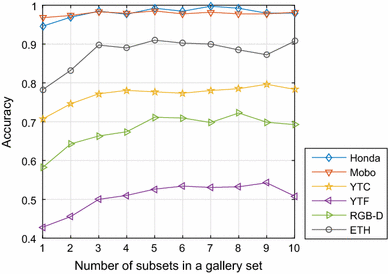
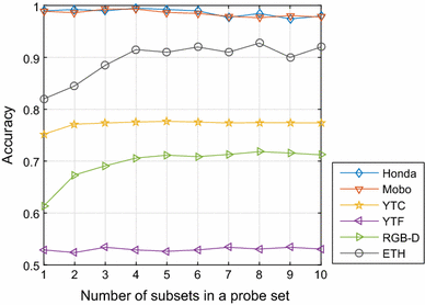
To determine the effect of c on the GCR representations, we evaluated the accuracy of ridge regression classifiers fit on six datasets using GCR representations with different values of c. Figure 11 shows the accuracy when c is fixed to 5 for the probe set representations and is varied for the gallery set representations, and Fig. 12 shows the accuracy when c is fixed to 5 for the gallery set representations and varied for the probe set representations. The reported accuracies are 10-fold cross-validated.

Fig. 12

Impact of c (the number of subsets in each probe set) on GCR in terms of classification accuracy where each gallery set is represented with five subsets

We see from Fig. 11 that the accuracy is low when c is small for the gallery set representations, and becomes relatively stable when c is in [3, 10]. This is reasonable, because when c is small, we are merging together image clusters and losing useful information, but when c is larger, we do not pay any accuracy price for potentially over-partitioning the image clusters. From Fig. 12, we find that the accuracy increases and then decreases as the number of clusters used to represent the probe sets increases. Here large c means that the probe set is over-segmented relative to the gallery sets, which makes the voting scheme more sensitive to outliers and violates the voting consistency (as discussed in Sect. 4) required in the prediction process. Based on these observations, we set c as 5 for the representations of both gallery and probe sets.

1.2 Trade-off Parameters $\lambda _1$, $\lambda _2$ and $\lambda _3$

There are three terms in the PSsR model (8). In this subsection, we will demonstrate the effect of the two regularizers, the second term ($\ell _2$-norm constraint on new representation) and the third term (group sparsity constraint on new representation).

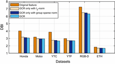
In the first experiment, we calculate the Davies–Bouldin index (DBI) (Davies and Bouldin 1979) of six datasets for four representations (the original pixel features, PSsR with only $\ell _2$-norm regularization (i.e., $\lambda _1=0$), PSsR with only group lasso regularization (i.e., $\lambda _2=0$), and PSsR with the full objective). The DBI measure simultaneously evaluates intra-cluster compactness and inter-cluster separation, and is defined as

$$\begin{aligned} DBI=\frac{1}{L}\sum _{i=1}^L\max _{i\ne j}\frac{C_i+C_j}{S_{i,j}} \end{aligned}$$

(39)

where $C_i=\frac{1}{n_i}\sum _{k=1}^{n_i}\Vert \varvec{x}_k - \varvec{\mu }_i\Vert _2$ measures the compactness of the ith category and $S_{i,j}=\Vert \varvec{\mu }_i - \varvec{\mu }_j\Vert _2$ measures the separation between the ith and jth categories. Here L is the number of classes, $\varvec{\mu }_i$ is the mean of the images in the ith class, and $n_i$ is the number of images in the ith class. Lower DBI values indicate that a representation is better able to capture intra- and inter-set relationships.

Fig. 13

The quality of four choices of features used to represent the all six datasets measured in terms of the Davies–Bouldin index (Davies and Bouldin 1979, the smaller the better)

Fig. 14

Effect of $\lambda _1$ and $\lambda _2$ on GCR in terms of classification accuracy for six datasets a Honda, b Mobo, c YTC, d YTF, e RGB-D and f ETH

The DBIs of four representations evaluated on the Honda video training dataset ($L=20$) are shown in Fig. 13. Clearly the lowest DBI value is obtained by the PSsR, which demonstrates that the collaborative nature of the GCR model as well as the mixture of group sparsity and $l_2$ penalties encourages learning representations that are discriminative and result in compact classes.

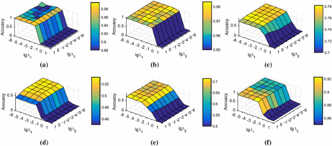
From the above results, it can be roughly seen that the parameters $\lambda _1$ and $\lambda _2$ control the trade-offs between group sparsity, ridge regularization, and the reconstruction loss in the PSsR objective (8). To demonstrate the effect of these parameters in detail, we conducted extensive experiments by varying $\lambda _1$ and $\lambda _2$ on six datasets, as shown in Fig. 14. Ridge regression is used and the accuracies reported are 10-fold cross-validated. For simplicity, we set $\lambda _1$ and $\lambda _2$ in the SSsR objective (9) to the same values as those used in the PSsR objective. Since the $\lambda _3$ parameter in the SSsR objective plays a similar role to $\lambda _2$, we take $\lambda _3 = \lambda _2.$

Both parameters took values in $\{10^{-6},10^{-5},\ldots ,10^{0},10^{1}\}$. It can be seen that GCR performs stably over a wide range of settings for $\lambda _1$ and $\lambda _2.$ In particular, the representations’ accuracy is insensitive to $\lambda _2.$ Note, however, that large values of $\lambda _1$ ($>10^{-2}$) tend to result in overly sparse coefficients, which leads to information loss and decreased accuracy. Based on these results, in all other experiments, we set $\lambda _1=10^{-3}$, $\lambda _2=10^{-1}$ and $\lambda _3=10^{-1}$.

The ridge-regression parameter used in fitting the RR and KRR classifiers (10) was tuned among the values $\{10^{-5}, 10^{-4},\ldots ,10^{3},10^{4}\}$. The experimental results show that the classification accuracy is insensitive to $\beta$. Thus we fix $\beta$ in our experiments (with both the RR and KRR classifiers) at $10^{-3}$.

References

Arandjelovic, O., Shakhnarovich, G., Fisher, J., Cipolla, R., & Darrell, T. (2005). Face recognition with image sets using manifold density divergence. In IEEE conference on computer vision and pattern recognition (Vol. 1, pp. 581–588). IEEE.
Bach, F., Jenatton, R., Mairal, J., Obozinski, G., et al. (2012). Structured sparsity through convex optimization. Statistical Science, 27(4), 450–468.
Boyd, S., Parikh, N., Chu, E., Peleato, B., & Eckstein, J. (2011). Distributed optimization and statistical learning via the alternating direction method of multipliers. Foundations and Trends in Machine Learning, 3(1), 1–122.
Cai, D., He, X., Han, J., & Huang, T. S. (2011). Graph regularized nonnegative matrix factorization for data representation. IEEE Transactions on Pattern Analysis and Machine Intelligence, 33(8), 1548–1560.
Cevikalp, H., & Triggs, B. (2010). Face recognition based on image sets. In IEEE conference on computer vision and pattern recognition (pp. 2567–2573). IEEE.
Chen, S., Sanderson, C., Harandi, M. T., & Lovell, B. C. (2013). Improved image set classification via joint sparse approximated nearest subspaces. In IEEE conference on computer vision and pattern recognition (pp. 452–459). IEEE.
Davies, D. L., & Bouldin, D. W. (1979). A cluster separation measure. IEEE Transactions on Pattern Analysis and Machine Intelligence, 1(2), 224–227.
Deng, W., & Yin, W. (2016). On the global and linear convergence of the generalized alternating direction method of multipliers. Journal of Scientific Computing, 66(3), 889–916.
Gross, R., & Shi, J. (2001). The CMU motion of body (mobo) database. Technical report.
Harandi, M. T., Sanderson, C., Shirazi, S., & Lovell, B. C. (2011). Graph embedding discriminant analysis on Grassmannian manifolds for improved image set matching. In IEEE conference on computer vision and pattern recognition (pp. 2705–2712). IEEE.
Hayat, M., Bennamoun, M., & An, S. (2014). Reverse training: An efficient approach for image set classification. In European conference on computer vision (pp. 784–799). Springer.
Hayat, M., Bennamoun, M., & An, S. (2015). Deep reconstruction models for image set classification. IEEE Transactions on Pattern Analysis and Machine Intelligence, 37(4), 713–727.
Hu, Y., Mian, A. S., & Owens, R. (2012). Face recognition using sparse approximated nearest points between image sets. IEEE Transactions on Pattern Analysis and Machine Intelligence, 34(10), 1992–2004.
Huang, Z., Wang, R., Shan, S., & Chen, X. (2014). Learning Euclidean-to-Riemannian metric for point-to-set classification. In 2014 IEEE conference on computer vision and pattern recognition (CVPR) (pp. 1677–1684). IEEE.
Kim, M., Kumar, S., Pavlovic, V., & Rowley, H. (2008). Face tracking and recognition with visual constraints in real-world videos. In IEEE conference on computer vision and pattern recognition (pp. 1–8). IEEE.
Kim, T. K., Kittler, J., & Cipolla, R. (2007). Discriminative learning and recognition of image set classes using canonical correlations. IEEE Transactions on Pattern Analysis and Machine Intelligence, 29(6), 1005–1018.
Lai, K., Bo, L., Ren, X., & Fox, D. (2011). A large-scale hierarchical multi-view RGB-D object dataset. In IEEE international conference on robotics and automation (pp. 1817–1824). IEEE.
Lee, K. C., Ho, J., Yang, M. H., & Kriegman, D. (2003). Video-based face recognition using probabilistic appearance manifolds. In IEEE conference on computer vision and pattern recognition (Vol. 1, pp 1–313). IEEE.
Lin, Z., Liu, R., & Su, Z. (2011). Linearized alternating direction method with adaptive penalty for low-rank representation. In Advances in neural information processing systems (pp. 612–620).
Lu, C. Y., Min, H., Zhao, Z. Q., Zhu, L., Huang, D. S., & Yan, S. (2012). Robust and efficient subspace segmentation via least squares regression. In Proceedings of the 12th European conference on computer vision (pp. 347–360). Springer.
Lu, J., Wang, G., Deng, W., Moulin, P., & Zhou, J. (2015). Multi-manifold deep metric learning for image set classification. In Proceedings of the IEEE conference on computer vision and pattern recognition (pp. 1137–1145).
Lu, J., Wang, G., & Moulin, P. (2013). Image set classification using holistic multiple order statistics features and localized multi-kernel metric learning. In IEEE international conference on computer vision (pp. 329–336). IEEE.
Mahmood, A., Mian, A., & Owens, R. (2014). Semi-supervised spectral clustering for image set classification. In Proceedings of the IEEE conference on computer vision and pattern recognition (pp. 121–128).
Ng, M. K., Wang, F., & Yuan, X. (2011). Inexact alternating direction methods for image recovery. SIAM Journal on Scientific Computing, 33(4), 1643–1668.
Parkhi, O. M., Vedaldi, A., & Zisserman, A. (2015). Deep face recognition. In British machine vision conference (Vol. 1, p. 6).
Razaviyayn, M., Hong, M., & Luo, Z. Q. (2013). A unified convergence analysis of block successive minimization methods for nonsmooth optimization. SIAM Journal on Optimization, 23(2), 1126–1153.
Saunders, C., Gammerman, A., & Vovk, V. (1998). Ridge regression learning algorithm in dual variables. In Proceedings of the 15th international conference on machine learning (pp. 515–521). Morgan Kaufmann.
Shakhnarovich, G., Fisher, J. W., & Darrell, T. (2002). Face recognition from long-term observations. In European conference on computer vision (pp. 851–865). Springer.
Simonyan, K., & Zisserman, A. (2014). Very deep convolutional networks for large-scale image recognition. arXiv preprint arXiv:14091556.
Tao, M., & Yuan, X. (2011). Recovering low-rank and sparse components of matrices from incomplete and noisy observations. SIAM Journal on Optimization, 21(1), 57–81.
Uzair, M., Mahmood, A., & Mian, A. (2014). Sparse kernel learning for image set classification. In Asian conference on computer vision (pp. 617–631). Springer.
Vidal, R. (2011). Subspace clustering. IEEE Signal Processing Magazine, 28(2), 52–68.
Viola, P., & Jones, M. J. (2004). Robust real-time face detection. International Journal of Computer Vision, 57(2), 137–154.
Wang, R., & Chen, X. (2009). Manifold discriminant analysis. In IEEE conference on computer vision and pattern recognition (pp. 429–436). IEEE.
Wang, R., Guo, H., Davis, L. S., & Dai, Q. (2012). Covariance discriminative learning: A natural and efficient approach to image set classification. In IEEE conference on computer vision and pattern recognition (pp. 2496–2503). IEEE.
Wang, R., Shan, S., Chen, X., & Gao, W. (2008). Manifold–manifold distance with application to face recognition based on image set. In IEEE conference on computer vision and pattern recognition (pp. 1–8). IEEE.
Wang, W., Wang, R., Huang, Z., Shan, S., & Chen, X. (2015). Discriminant analysis on Riemannian manifold of Gaussian distributions for face recognition with image sets. In Proceedings of the IEEE conference on computer vision and pattern recognition (pp. 2048–2057).
Wolf, L., Hassner, T., & Maoz, I. (2011). Face recognition in unconstrained videos with matched background similarity. In IEEE conference on computer vision and pattern recognition (pp. 529–534). IEEE.
Yang, M., Zhu, P., Van Gool, L., & Zhang, L. (2013). Face recognition based on regularized nearest points between image sets. In 2013 10th IEEE international conference and workshops on automatic face and gesture recognition (FG) (pp. 1–7). IEEE.
Yuan, M., & Lin, Y. (2006). Model selection and estimation in regression with grouped variables. Journal of the Royal Statistical Society: Series B (Statistical Methodology), 68(1), 49–67.
Zhang, D., Yang, M., & Feng, X. (2011). Sparse representation or collaborative representation: Which helps face recognition? In Proceedings of the 13th international conference on computer vision (pp. 471–478). IEEE.
Zhu, P., Zhang, L., Zuo, W., & Zhang, D. (2013). From point to set: Extend the learning of distance metrics. In 2013 IEEE international conference on computer vision (ICCV) (pp. 2664–2671). IEEE.
Zhu, P., Zuo, W., Zhang, L., & Shiu, S. C. (2014). Image set based collaborative representation for face recognition. IEEE Transactions on Information Forensics and Security, 9(7), 1120–1132.
Zou, H., & Hastie, T. (2005). Regularization and variable selection via the elastic net. Journal of the Royal Statistical Society: Series B (Statistical Methodology), 67(2), 301–320.
Zou, H., Zhu, J., Hastie, T., et al. (2008). New multicategory boosting algorithms based on multicategory fisher-consistent losses. The Annals of Applied Statistics, 2(4), 1290–1306.
Acknowledgements
Funding was provided by National Natural Science Foundation of China (Grant Nos. 61632004, 61773050) and Opening Project of Beijing Key Lab of Traffic Data Analysis and Mining (Grant No. BKLTDAM2017001).
Author information
Authors and Affiliations
Corresponding author
Additional information
Communicated by M. Hebert.