Online signal extraction by robust regression in moving windows with data-adaptive width selection

Abstract

Online (also ‘real-time’ or ‘sequential’) signal extraction from noisy and outlier-interfered data streams is a basic but challenging goal. Fitting a robust Repeated Median (Siegel in Biometrika 69:242–244, 1982) regression line in a moving time window has turned out to be a promising approach (Davies et al. in J. Stat. Plan. Inference 122:65–78, 2004; Gather et al. in Comput. Stat. 21:33–51, 2006; Schettlinger et al. in Biomed. Eng. 51:49–56, 2006). The level of the regression line at the rightmost window position, which equates to the current time point in an online application, is then used for signal extraction. However, the choice of the window width has a large impact on the signal extraction, and it is impossible to predetermine an optimal fixed window width for data streams which exhibit signal changes like level shifts and sudden trend changes. We therefore propose a robust test procedure for the online detection of such signal changes. An algorithm including the test allows for online window width adaption, meaning that the window width is chosen w.r.t. the current data situation at each time point. Comparison studies show that our new procedure outperforms an existing Repeated Median filter with automatic window width selection (Schettlinger et al. in Int. J. Adapt. Control Signal Process. 24:346–362, 2010).

Appendices

Appendix A: Monte Carlo approximation of $\hat{\mbox {V}} ( \ell,1 )$ and $\hat{\mbox {V}} ( r,1 )$

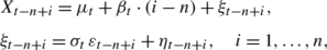
We approximate $v_{n} := \hat{\mbox {V}} ( n,1 )$ for n=5,…,300 by the empirical variance of RM slopes which are estimated on samples coming from

$$ X_{t-n+i} = \mu_t + \beta_t \cdot(i-n) + \varepsilon_{t-n+i},\quad i = 1,\ldots,n, $$

with standard normal i.i.d. errors ε _t−n+i ∼N(0,1). W.l.o.g. we set μ _t =β _t =0 because of the regression equivariance of the RM slope (Rousseeuw and Leroy 1987), i.e. X _t−n+i =ε _t−n+i .

We generate time series (x _t ) consisting of 100,000+300−1=100,299 observations. Then for each n=5,…,300 we move a time window {t−n+1…,t} over the time series, starting at time point t=300. Hence, for each n we obtain 100,000 RM slopes, and v _n is the empirical variance computed on these 100,000 RM slopes. Due to this time series design the RM slopes are autocorrelated, as they are in practice. However, in another simulation study we also approximated the RM slope variance for independent samples. These estimates are comparable to those obtained by the time series design.

As was to be expected, the variance of the RM slope decreases monotonically with increasing window size n, see Fig. 9. In order to obtain approximations v _n for n>300, we model the relationship between n and v _n and find that the function

$$ v(n)= 4.77 \cdot10^{-7} + 17.71 \cdot n^{-3} $$

gives an appropriate fit with standard error 0.0004 and coefficient of determination 0.9983.

Fig. 9

Empirical variance of 100,000 RM slopes estimated on standard normal samples of size n=5,…,50

Appendix B: The empirical distribution of the SCARM test statistic

This Monte Carlo study analyzes the distribution of the SCARM test statistic T _t under the null hypothesis. That is, we compute T _t on samples x _t that come from model (4):

where we set μ _t =β _t =0 w.l.o.g. due to the regression equivariance of the RM slope. First of all we consider standard normal errors, as assumed in the theoretical development of the SCARM test, i.e. η _t−n+i =0 and $\sigma_{t} \, \varepsilon_{t-n+i} \sim N(0,\sigma_{t}^{2})$, and w.l.o.g. we set σ _t =1. We generated 10,000 samples of length n=ℓ+r for r∈{5,10,…,100} and ℓ∈{r,r+5,…,100}. Thus, for any combination ℓ,r we obtained 10,000 realizations of the SCARM test statistic T _t .

We find that the distribution of the SCARM test statistic can be well approximated by a t-distribution with f degrees of freedom, where f depends on ℓ and r. For each combination (ℓ,r), we compare the empirical α- and (1−α)-quantiles, α=0.01,0.02,…,0.05, of the SCARM test statistic to the corresponding theoretical quantiles of a t-distribution with degrees of freedom f=0.1,0.2,…,100, in order to find a suitable f for each combination (ℓ,r). For each (ℓ,r)-combination, we choose that f that minimizes the mean absolute difference between the empirical and the theoretical quantiles. Table 4 lists the suitable degrees of freedom f(ℓ,r) for r∈{5,10,…,50} and ℓ∈{r,r+5,…,50}. The degrees of freedom f, and thus the quantiles t _f,α/2 and t _f,1−α/2, are expected to be monotonically increasing in ℓ and r. However, this is not true for the approximations of f(ℓ,r) in Table 4. Therefore, for r∈{5,…,100} and ℓ∈{r,…,100} we set

$$ f(\ell,r) = \min\limits _{\ell' \geq\ell} \min\limits _{r' \geq r} \bigl\{ f\bigl( \ell',r'\bigr) \bigr\}, $$

(20)

with r′∈{5,10,…,50} and ℓ′∈{r′,r′+5,…,50} to achieve monotonic degrees of freedom f and thus monotonic critical values t _f,α/2 and t _f,1−α/2. By taking the minimum in (20) we decide for larger absolute critical values in order that the test keeps the chosen level of significance α. If ℓ or r is larger than 100, we use standard normal quantiles as critical values.

Table 4 Approximation of the SCARM test statistic distribution by a t-distribution: suitable degrees of freedom f(ℓ,r)

2.1 B.1 Other error types

We further investigate the distribution of T _t for heavy-tailed, skewed, and contaminated errors ξ _t−n+i , in particular:

• Noise type 1: heavy-tailed errors from a standardized t-distribution with three degrees of freedom;

• Noise type 2: skewed errors from a standardized Weibull distribution with scale and shape parameter two and one;

• Noise type 3: standard normal errors with 10 % contamination from N(10,1);

• Noise type 4: standard normal errors with 10 % contamination from $N(0,\sigma_{t}^{2}=100)$.

Table 5 gives the empirical (1−α/2)-quantiles, α=0.01,0.005,0.001, of the computed SCARM test statistics for the four noise types and for different combinations (ℓ,r). Furthermore, the table lists the quantiles of the t _f(ℓ,r)-distribution which are used as critical values for test decision. The empirical quantiles are generally lower than the t _f -quantiles that are used for test decision, except for (ℓ,r)=(10,10) and given the skewed noise type 2. That is, the test keeps the chosen level of significance, even if the noise is heavy-tailed or contaminated. However, if the noise is skewed, ℓ and r should both not be too small.

Table 5 Quantiles of a t _f(ℓ,r) distribution and empirical quantiles of the SCARM test statistic computed on different types of noise

References

Bernholt, T., Fried, R.: Computing the update of the repeated median regression line in linear time. Inf. Process. Lett. 88(3), 111–117 (2003)
Bernholt, T., Fried, R., Gather, U., Wegener, I.: Modified repeated median filters. Stat. Comput. 16, 177–192 (2006)
Borowski, M., Schettlinger, K., Gather, U.: Multivariate real time signal processing by a robust adaptive regression filter. Commun. Stat., Simul. Comput. 38(2), 426–440 (2009)
Chen, C., Chan, J., Gerlach, R., Hsieh, W.: A comparison of estimators for regression models with change points. Stat. Comput. 21(3), 395–414 (2011)
Davies, P., Gather, U.: Breakdown and groups. Ann. Stat. 33(3), 977–1035 (2005)
Davies, P., Fried, R., Gather, U.: Robust signal extraction for on-line monitoring data. J. Stat. Plan. Inference 122, 65–78 (2004). Special Issue: Contemporary Data Analysis: Theory and Methods in Honor of John W. Tukey
Fried, R.: Robust filtering of time series with trends. J. Nonparametr. Stat. 16(3–4), 313–328 (2004)
Fried, R.: On the robust detection of edges in time series filtering. Comput. Stat. Data Anal. 52, 1063–1074 (2007)
Fried, R., Bernholt, T., Gather, U.: Repeated median and hybrid filters. Comput. Stat. Data Anal. 50(9), 2313–2338 (2006)
Fried, R., Einbeck, J., Gather, U.: Weighted repeated median smoothing and filtering. J. Am. Stat. Assoc. 102, 1300–1308 (2007)
Fried, R., Schettlinger, K., Borowski, M.: Getting started with robfilter (2012a). http://www.statistik.tu-dortmund.de/1543.html
Fried, R., Schettlinger, K., Borowski, M., robfilter: Robust time series filters (2012b). http://CRAN.R-project.org/package=robfilter, with manual
Gather, U., Fried, R.: Methods and algorithms for robust filtering. In: Proceedings in Computational Statistics (COMPSTAT 2004), pp. 159–170. Physica, Heidelberg (2004)
Gather, U., Schettlinger, K., Fried, R.: Online signal extraction by robust linear regression. Comput. Stat. 21, 33–51 (2006)
Gelper, S., Schettlinger, K., Croux, C., Gather, U.: Robust online scale estimation in time series: a model-free approach. J. Stat. Plan. Inference 139(2), 335–349 (2009)
Rousseeuw, P., Hubert, M.: Regression-free and robust estimation of scale for bivariate data. Comput. Stat. Data Anal. 21(1), 67–85 (1996)
Rousseeuw, P., Leroy, A.: Robust Regression and Outlier Detection. Wiley, New York (1987)
Schettlinger, K.: Signal and variability extraction for online monitoring in intensive care. Ph.D. thesis, Faculty of Statistics, TU Dortmund University (2009)
Schettlinger, K., Fried, R., Gather, U.: Robust filters for intensive care monitoring: beyond the running median. Biomed. Eng. 51, 49–56 (2006)
Schettlinger, K., Fried, R., Gather, U.: Real time signal processing by adaptive repeated median filters. Int. J. Adapt. Control Signal Process. 24, 346–362 (2010)
Siegel, A.: Robust regression using repeated medians. Biometrika 69, 242–244 (1982)
Ylvisaker, D.: Test resistance. J. Am. Stat. Assoc. 72, 551–556 (1977)
Acknowledgements
The financial support of the Deutsche Forschungsgemeinschaft (SFB 823, Statistical modelling of nonlinear dynamic processes) is gratefully acknowledged. The authors thank the referees for their helpful comments.
Author information
Authors and Affiliations
Corresponding author