Runtime verification of real-time event streams under non-synchronized arrival

Abstract

We study the problem of online runtime verification of real-time event streams. Our monitors can observe concurrent systems with a shared clock, but where each component reports observations as signals that arrive to the monitor at different speeds and with different and varying latencies. We start from specifications in a fragment of the TeSSLa specification language, where streams (including inputs and final verdicts) are not restricted to be Booleans but can be data from richer domains, including integers and reals with arithmetic operations and aggregations. Specifications can be used both for checking logical properties and for computing statistics and general numeric temporal metrics (and properties on these richer metrics). We present an online evaluation algorithm for the specification language and a concurrent implementation of the evaluation algorithm. The algorithm can tolerate and exploit the asynchronous arrival of events without synchronizing the inputs. Then, we introduce a theory of asynchronous transducers and show a formal proof of the correctness such that every possible run of the monitor implements the semantics. Finally, we report an empirical evaluation of a highly concurrent Erlang implementation of the monitoring algorithm.

1 Introduction

We study the online runtime verification of real-time event streams and signals that arrive at different speeds and with different and varying delays to the monitor.

Runtime verification (RV) is an applied formal technique for software reliability. In contrast to static verification, in RV, only one trace of the system under scrutiny is considered. Thus, RV sacrifices completeness guarantees to obtain an immediately applicable and formal extension of testing and debugging. Central problems in runtime verification are (1) how to generate monitors from formal specifications and (2) how to evaluate these monitors against input traces from the running system (for a more detailed overview of RV, see Havelund and Goldberg (2005) and Leucker and Schallhart (2009) for surveys and Bartocci and Falcone (2018) for a reference book).

In this paper, we study how to perform runtime verification of concurrent systems whose components share a global clock that is used to time-stamp their internal events. These events emitted by the components are sent to the monitor at different speeds, and arrive to the monitor with different and varying delays. This assumption is inspired by the timed-asynchronous model of computation (Cristian and Fetzer 1999) from distributed computing, where distributed components have a globally synchronized clock (like in synchronous distributed computing) but the messages can experience unbounded delays (like in asynchronous distributed computing). This assumption is common, for example, when observing embedded systems or when observing low-level execution traces of software running on multi-core processors, which is our main target practical application. At the low-level software analysis, the signals that these systems emit are real-time signals that remain constant between two observations, also known as piece-wise constant signals or timed event-streams.

We are targeting embedded and cyber-physical systems using multi-core processors and thus are generating a huge amount of events. Consider a producer-consumer setting where multiple producers and consumers are running on different cores of a multi-core processor. The producers write events into a ring buffer and the consumers read and process those values, where every value is only allowed to be read once. Such a system would generate a huge amount of events like when a value is inserted into the ring buffer, one is read from it, one is processed, pointer which point at different buffer cells are moved, and so on. Processing all those events to, for example, find values which are read twice or pointers that are not moved in time which means that producers or consumers interfere each other needs a fast monitoring infrastructure which can process as many events as possible in parallel.

As described before, we are interested in online monitoring, which is performed while the system is running (as opposed to offline monitoring through post-mortem analysis of dumped traces). The target application of low-level software analysis of embedded systems also requires non-intrusive monitoring, meaning that the monitoring activity cannot perturb the execution of the system under observation. To achieve non-intrusiveness, the monitoring infrastructure uses some hardware capabilities, like processor debug interfaces, to obtain runtime information without instrumenting the code while the concurrent system executes. This information is dispatched to an external monitoring executing infrastructure that executes outline by reconstructing the path the execution took through the source code (as opposed to inlining the monitors within the system itself which is common in runtime verification for high-level software). See Leucker (2011) for a definition and classification of these RV concepts.

In this paper, we study the problem of monitoring under the non-synchronized arrival of real-time event streams, that is: (1) all events from all components are time-stamped according to the global clock, (2) events from a given component arrive to monitor ordered according to their time-stamp (locally ordered streams), but (3) events from different components do not necessarily arrive in the order of their time-stamps (non globally ordered streams).

Since the order and time at which events are processed are both important, we introduce here the explicit distinction between system time and monitor time. System time refers to the moments at which events are produced within the observed system, and the implied ordering between these events. These instants are captured by the synchronized global clock, which is used to time-stamp events by the instrumentation of the system under analysis. Monitor time refers to the instants at which events arrive at the monitor and when these events are processed to produce verdicts. The order in which arrival, processing and generation of outputs happen in the monitor depends not only on the implementation of the monitor but also on the arrival time and order of the input events.

The semantics of the specification languages to express monitors are typically defined in two styles. First, denotational semantics associate (unique) output streams of values for given input streams of values. The time in this semantics only verse about system time, as denotational semantics do not reason about when these outputs are produced. Second, operational semantics explain how the output streams are incrementally produced from given input streams. Even though the output streams generated must coincide with the denotational semantics (ultimately the streams must be the same), two operational semantics can differ on the instant (monitoring time) at which each piece of the output is produced. That is, the correctness of the monitoring process is determined by the system time and the values observed, while the instants at which the monitor can produce the output in an incremental fashion is determined by the monitor time. For example, a monitor that awaits for the whole input to be received before producing any output is correct but it is sometimes preferable to have a monitor that produces as much output as possible after every input event is received.

Event streams from hardware processors, like in embedded or cyber-physical systems possibly using multi-core processors, come at very high speeds, which imposes the additional requirement of crafting highly efficient monitoring implementations. We explore in this paper software monitors that can exploit the parallelism available in modern multi-core platforms, while still formally guaranteeing the correctness of the monitors such that we can process incoming events online much faster and can handle more incoming events. To effectively exploit the parallelism, these monitors must tolerate the non-synchronized arrival of events and progress as much as possible with only events from some sources.

Our solution for this problem starts from a specification language based on stream runtime verification. Stream runtime verification (SRV) is very appealing as an approach for our purposes, because the dependencies between streams allow to decompose specifications into components that can be executed concurrently and asynchronously. We use here an acyclic fragment of the TeSSLa specification language (Convent et al. 2018), an incarnation of SRV for real-time event streams. We call this fragment TeSSLa_a. TeSSLa stands for Temporal Stream-Based Specification Language, and has already been used for creating monitors in FPGA hardware in Decker et al. (2018) and Decker et al. (2017). Our acyclic fragment TeSSLa_a restricts TeSSLa to non-recursive specifications, which means that no cycles are allowed in a specification. The functionality that recursion allows with a few core operators in TeSSLa is encapsulated in TeSSLa_a in a collection of building blocks. This allows us to build in this paper a simpler asynchronous evaluation algorithm, for TeSSLa_a as a software monitor. In this solution, a specification is translated into a software monitor whose components can execute asynchronously in parallel communicating using message queues. Each stream defined in the specification is thus translated individually. This compositional operational semantics brings a lot of potential to exploit algorithmic advantages beyond the exploitation of concurrency that we show here, like for example monitoring.

Related work

Early specification languages for RV were based on their counterparts in static verification, typically logics like LTL (Manna and Pnueli 1995) or past LTL adapted for finite paths (Bauer et al. 2011; Eisner et al. 2003; Havelund and Roşu 2002). Similar formalisms proposed are based on regular expressions (Sen and Roşu 2003), timed regular expressions (Asarin et al. 2002), rule-based languages (Barringer et al. 2004), or rewriting (Roşu and Havelund 2005). Stream runtime verification, pioneered by the tool LOLA (D’Angelo et al. 2005), is an alternative to define monitors using streams. In SRV, one describes the dependencies between input streams of values (observable events from the system under analysis) and defined streams (alarms, errors, and output diagnosis information). These dependencies can relate the current value of a depending stream with the values of the same or other streams at the present moment, in past instants (like in past temporal formulas), or in future instants. In SRV, there is a clean separation between the evaluation algorithms—that exploit the explicit dependencies between streams—and the data manipulation—expressed by each individual operation.

SRV allows to generalize well-known evaluation algorithms from runtime verification to perform collections of numeric statistics from input traces. SRV resembles synchronous languages (Caspi and Pouzet 1996)—like Esterel (Berry 2000), Lustre (Halbwachs et al. 1987), or Signal (Gautier et al. 1987)—but these systems are causal because their intention is to describe systems and not observations, while SRV removes the causality assumption allowing to refer to future values. Another related area is functional reactive programming (FRP) (Eliot and Hudak 1997), where reactive behaviors are defined using functional programs as building blocks to express reactions. As with synchronous languages, FRP is a programming paradigm and not a monitoring specification language, so future dependencies are not allowed in FRP. On the other hand, SRV was initially conceived for monitoring synchronous systems, where the execution happens in cycles (see Bozelli and Sánchez 2014; Goodloe and Pike 2010; Pike et al. 2010) and not for real-time streams. The semantics of temporal logics can be defined using declarative dependencies between streams of values (see, for example, temporal testers (Pnueli and Zaks 2006) for LTL), which has been implemented for example in the tool R2U2 (Reinbacher et al. 2014). Likewise, the semantics of signal temporal logic (STL) (Donzé et al. 2012; Maler and Nickovic 2004) is defined in terms of the relation between a defined signal and the signals for its sub-expressions, based on metric interval temporal logic (Alur et al. 1996).

The specification language TeSSLa_a that we use extends SRV with support for real-time piece-wise constant signals. Most previous approaches to SRV assume synchronous sampling and synchronous arrivals of events in all input streams. It is theoretically feasible, at least in some cases, to reduce the setting in this paper to synchronous SRV (for example by assuming that all samples are made at instants are multiple of a minimum quantum delay, and executing the specification synchronously after every delay). However, the fast arrival of events would render such an approach impractical due to the large number of processing steps that would be required. That is, the monitor must be able to execute efficiently both at times of spread events and also under fast bursts. There are extensions of SRV for real-time signals, most notably RTLola (Faymonville et al. 2019; Baumeister et al. 2019) and Striver (Gorostiaga and Sánchez 2018). However, all the monitoring algorithms proposed and implemented for these logics, similarly to full TeSSLa, are not able to exploit concurrency and asynchronous evaluation. Moreover, the correctness of the operational semantics of these formalisms requires synchronous arrivals. Figure 1 summarizes the main SRV tools and features.

Fig. 1

Summary of features of stream runtime verification tools and languages

There are other assumptions in different target application domains that differ from the assumptions here. For example, for network monitoring (a target of Faymonville et al. 2016), it is reasonable to consider that input events modelled as a single source can arrive at different input “ports”, which must be processed in parallel. In the work in this paper, a single source arrives from a component of low-level embedded software through the instrumentation infrastructure, so it always arrives at single port and locally ordered. Also, the assumption on the system differs from the truly distributed nature of the problem of predicate detection in distributed systems (Chase and Garg 1998), where a global clock is not assumed to be available to the components of the system.

STL has also been used to create monitors on FPGAs (Jaksic et al. 2015) and for monitoring in different application areas (see for example Jaksic et al. 2016; Selyunin et al. 2016). However, the assumptions of STL on the signals are different than those of ours, because the goal of STL is to analyze arbitrary continuous signals and not necessarily changes from digital circuits with accurate clocks. Sampling ratios and sampling instants are important issues in STL, while the signals we assume here are accurately represented by the stream of events at the changing points of the signal. In timed regular expressions (TRE) (Asarin et al. 2002), the signals are also assumed to be piece-wise constant. Additionally, our framework can handle much richer data domains of data and verdicts than TREs and STL.¹ TREs have been combined with STL (Selyunin et al. 2017) to get the advantages of both domains but again the signals analyzed are not necessarily piece-wise constant. Consequently, the results are approximate and sampling becomes, again, an important issue.

Contributions

In summary, the contributions of this paper are as follows:

• 1. A method for the systematic generation of parallel and asynchronous online monitors for software monitoring of TeSSLa_a specifications. These monitors handle the non-synchronized arrival of events from different input stream sources.

• 2. A computational model for proving correctness of asynchronous concurrent monitors, introduced in Section 3, which enables to study a concurrent online evaluation algorithm for TeSSLa_a specifications.

• 3. A prototype implementation developed in Erlang, described in Section 4, and an empirical evaluation.

• 4. The precise syntax and semantics of TeSSLa_a, an acyclic fragment of TeSSLa, presented in Section 2, including the core and library functions.

Terminology

To clarify, we summarize here the terminology used in the rest of the paper:

• Real-time event streams: Our model of streams is that of real-time event streams, where streams are sequences of events. Each event contains a value (of the appropriate domain of the stream) and a time-stamp from a real-time domain. Each event is stamped in increasing with respect to previous events in the stream. Also, we assume that streams are non-Zeno, which means that for every time interval, there is a finite number of events with a time-stamp within the interval.

• Piece-wise constant signals: These are continuous signals that remain constant between the points of change, and that only have a finite number of points of change in any given time interval. Piece-wise constant signals and event streams are equivalent models of data streams.

• Locally ordered streams: A monitoring infrastructure guarantees locally ordered streams when timed-event streams that arrive to the monitor from a given component arrive in order of their time-stamps. In this work, we assume locally ordered streams.

• Globally ordered streams: a monitoring infrastructure that guarantees that events arrive to the monitor in order of their time-stamps even when these events come from different concurrent components. In this work, we do not assume globally ordered streams.

• Non-synchronized arrival: We use non-synchronized arrival to refer to locally ordered but non-globally ordered monitoring infrastructure.

• System time: This refers to the line of time of the shared global clock that is used to time-stamp events.

• Monitor time: The moments at which actions take place in the monitor. For example, the arrival of an event to the monitor or the instant of generation of an output from the monitor.

• Evaluation engine: An executable monitor expressed as a collection of computational nodes that can execute in parallel and asynchronously and communicate through message passing using queues.

• Computational node: Each of the elements (sometimes also called actors) of an evaluation engine.

Journal version

An earlier version of this paper appeared in Leucker et al. (2018), in the Proceedings of the 33rd Symposium on Applied Computing (SAC’18). This paper contains the following additional contributions: Section 2 now contains a full description of the TeSSLa_a language, as well as the formal semantics of each operator and the operational semantics of the implementation of each building block. Section 3 now contains a revisited and extended version of evaluation engines that encode the operational semantics of online monitors and that now consider bounded queues as well as unbounded queues. This section also includes a model of computation that can handle unbounded streams as ω-words. New theorems and full proofs of all results are now presented, including the proof that a fair scheduler is all that is needed to guarantee that all concurrent monitor executions preserve the denotational semantics. The empirical evaluation in Section 4 has also been extended to a larger study that illustrates how the implementation allows to exploit parallelism automatically. Finally, the tool chain is now described in Section 4.3.

2 Syntax and semantics of TeSSLa_a

We describe in this section the real-time specification language TeSSLa_a.² We first present some preliminaries, and then introduce the syntax and semantics.

2.1 Preliminaries

We use two types of stream models as underlying formalism: piece-wise constant signals and event streams. We use $\mathbb {T}$ for the time domain (which can be $\mathbb {N}$, $\mathbb {Q}$, $\mathbb {R}$, etc), and D for the collection of data domains (Booleans, integers, reals, etc). Values from these data domains model observations and the output verdicts produced by the monitors. In this manner, output verdicts can be numerical statistics or complex data collected from the trace.

Definition 1 (Event stream)

An event stream is a partial function $\eta : \mathbb {T} \rightharpoondown D$ such that $E(\eta ) := \{t \in \mathbb {T} \mid \eta (t) \text { is defined}\}$ does not contain bounded infinite subsets.

The set of all event streams is denoted by $\mathcal {E}_{D}$. The set E(η) is called the set of event points of η. When η is not defined at a time point t, that is $t \in \mathbb {T} \setminus E(\eta )$, we write η(t) = ⊥.

We use ⊤ as the “unit” value (the only value in a singleton domain). A finite event stream η can be naturally represented as a timed word, that is, a sequence $s_{\eta } = (t_{0},\eta (t_{0}))(t_{1},\eta (t_{1})){\dots } \in (E(\eta ) \times D)^{*}$ ordered by time (t_i < t_i+ 1) that contains a D value at all event points.

The second type of stream model that we consider is piece-wise constant signals, which have a value at every point in time. These signals change value only at a discrete set of positions and remain constant between two change points. This allows a smoother definition of the functions available in TeSSLa_a and delivers a more convenient model to the user.

Definition 2 (Signal)

A signal is a total function $\sigma : \mathbb {T} \rightarrow D$ such that the set of change points

$$ {\Delta}(\sigma) := \{t \in \mathbb{T} \mid \nexists t^{\prime} < t: \forall t^{\prime\prime}. t^{\prime} < t^{\prime\prime} < t: \sigma(t) = \sigma(t^{\prime\prime})\} $$

does not contain bounded infinite subsets.

The set of all signals is denoted by $\mathcal {S}_{D}$. Every piece-wise constant signal can be exactly represented by an event stream that contains the change points of the signal as events, and whose value is the value of the signal after the change point. Hence, one can convert signals into event streams and vice-versa. Note that while in STL, sampling provides an approximation of fully continuous signals, in TeSSLa_a, event streams represent piece-wise constant signals with perfect accuracy.

Example 1

Consider the following streams e, s, and e2, where e and e2 are interpreted as event streams and s as a signal.

The signal s has been created from e by using the value of the last event on e as value, with a default value 0. In turn, stream e2 is defined as the changes in value of s. When converting signals into event streams, only events that represent actual changes are generated.

We want to define monitors that run concurrently and asynchronously with the system under analysis, and we want to reason about their correctness. Then, it is very important to distinguish between the time at which an event e happens and that is used to time-stamp the event, and the time at which a given monitor receives the event. We use t(e) for the time of the occurrence of the event in the system, and rt(e) for the time at which e reaches the specified monitor.

Definition 3 (In-order streams)

A stream s is called in-order whenever for every two events e and $e^{\prime }$, ${t}(e) < {t}(e^{\prime }) \Rightarrow rt(e) < rt(e^{\prime })$ holds.

2.2 Syntax of TeSSLa_a

We begin with an example to illustrate a simple TeSSLa_a specification. Specifications are declarative, defining streams in terms of other streams, and ultimately in terms of input streams. Streams marked as out are the verdict of the monitor and their values will be reported to the user.

Example 2

Consider the following TeSSLa_a specification:

The first two lines define two input streams, e (an event stream without values) and s (a signal of integers). The Boolean signal comp is true if the number of events of e (denoted by eventCount(e)) is greater than the current value of s, and false otherwise. The Boolean signal allowed is true when there is an event that has not been filtered out from e in the interval [− 1,+ 1] around the current instant. The function filter eliminates an event if the Boolean signal as the second parameter is false. Finally, the Boolean signal ok is false whenever s is greater than 5 and allowed is false. Consider the input shown in the box below.

When allowed is true, so will be ok. The signal ok will also be true as long as s is lower than 5. When s becomes 7, not enough events have happened on e and then comp is false. Consequently, no event is left through the filter and allowed is false too. But because s is greater than 5, ok becomes false. When s is set back to 6 and more events on e have happened, allowed becomes true again.

The basic syntax of a TeSSLa_a specification spec is

$$ \begin{array}{@{}rcl@{}} {\mathit{spec}} \text{ ::= } &&\texttt{\textbf{define }} {\mathit{name}}[\texttt{\textbf{:}}\ stype] \texttt{\textbf{ := }} texpr \mid \texttt{\textbf{out }} {\mathit{name}} \mid \\ && \texttt{\textbf{in }} {\mathit{name}}\texttt{\textbf{:}}\ stype \mid {\mathit{spec}} {\mathit{spec}}\\ texpr \text{ ::= } && expr[\texttt{\textbf{:}}\ type] \\ expr \text{ ::= } && name \mid literal \mid name\texttt{\textbf{(}}texpr(\texttt{\textbf{, }}texpr)^{*}\texttt{\textbf{)}}\\ type \text{ ::= } && btype \mid stype \\ stype \text{ ::= } && \texttt{\textbf{Signal<}}btype\texttt{\textbf{>}} \mid \texttt{\textbf{Events<}}btype\texttt{\textbf{>}} \end{array} $$

A name is a non-empty string. Basic types btype cover typical types found in programming and verification like Int, Float, String, or Bool. One of the main contributions of SRV is to generalize existing monitoring algorithms for logics (that produce Boolean verdicts) to algorithms that compute values from richer domains (D’Angelo et al. 2005; Sánchez 2018). The production in introduces input stream variables, and define introduces defined stream variables (also called output variables). Given a specification φ, we use I for the set of input variables and O for the set of output variables, and write φ(I,O). For example, in Example 2 above, I = {e,s} and O = {comp,allowed,ok}. The marker out is used to denote those output variables that are the result of the specification and will be reported to the user. Each defined variable x is associated with a defining equationE_x given by the expression on the right-hand side of the := symbol. Literals literal denote explicit values of basic types such as integers $-1,0,1,2,\dots$, floating point numbers 0.1,− 3.141593 or strings "foo", "bar" (enclosed in double quotes). Available basic types and literal representation are implementation dependent. A flat specification is one such that every defining equation E_x is either a name, a literal, or an expression of the form f(x₁,…,x_n) where x_i are all stream names. Every specification can be transformed into an equivalent flat specification by introducing additional variables for each sub-expression.

We expand the syntax of basic TeSSLa_a by adding builtin functions, user defined macros and timing functions.

$$ \begin{array}{@{}rcl@{}} {\mathit{name}} &\text{ ::= } & {\mathit{defName}} \mid {\mathit{timingFun}} \mid {\mathit{builtinFun}} \mid {\mathit{macro}} \\ {\mathit{timingFun}} &\text { ::= } & {\textit{delay}} \mid {\textit{shift}} \mid {\textit{within}} \end{array} $$

A defName is simply a name of a previously defined stream or constant. Timing functions allow to describe timing dependencies between streams. The function delay delays the values of a signal (or events of an event stream) by a certain amount of time. The function shift shifts the values of an event stream one unit into the future, that is, the first event becomes the second event, etc. The function within defines a signal which is true as long as some event of the given stream exists within the specified interval.

Macros are user-defined functions identified by the construct fun. Macros can be expanded at compile time using their definition on a purely syntactical level because macros are not recursive. Macros can be defined with the following production, which is added to spec:

$$ \begin{array}{@{}rcl@{}} {\textit{macro}} \text{ := } & {\texttt{\textbf{fun}}} {\mathit{name}} \texttt{\textbf{(}}{\mathit{name}}(\texttt{\textbf{, }} {\mathit{name}} )^{*}\texttt{\textbf{)}} \texttt{\textbf{ := }} {\textit{texpr}} \mid {\textit{macro}} {\textit{macro}} \end{array} $$

where the texpr can use the names of the macro arguments.

Example 3

An example of a macro has already been used in the Example 2 because implies is not a builtin function. Instead, implies is defined by the following macro:

The expressivity of TeSSLa_a is obtained by the use a set of builtin functions. We first define in Section 2.3 the semantics of the temporal core of TeSSLa_a, which is enough to define the semantics of TeSSLa_a in Section 2.4. Then, we give semantics of the non-temporal building blocks in Section 2.5.

2.3 Semantics of timing functions

There are three timing functions: delay, shift, and within. The function delay is overloaded for signals

$$ \begin{array}{@{}rcl@{}} {\textit{delay}} &:& \mathcal{S}_{D} \times \mathbb{T} \times D \rightarrow \mathcal{S}_{D} \\ {\textit{delay}}(\sigma,d,v)(t) & =& \left\{\begin{array}{lllll} \sigma(t-d) & \text{if } t-d \geq 0\\ v & \text{otherwise} \end{array}\right. \end{array} $$

and for event streams

$$ \begin{array}{@{}rcl@{}} {\textit{delay}} &:& \mathcal{E}_{D} \times \mathbb{T} \rightarrow \mathcal{E}_{D} \\ {\textit{delay}}(\eta,d)(t) & =& \left\{\begin{array}{lllll} \eta(t-d) & \text{if } t-d \geq 0\\ \bot & \text{otherwise} \end{array}\right. \end{array} $$

The function delay delays a signal or an event stream by a given amount of time. Since signals must always carry a value, a value v is provided as default in case the signal being delayed is fetched outside its domain. For event streams, the occurrence of each event is delayed by the indicated amount of time (and an undefined value is used if the original event is fetched outside the boundaries). In other words, an input event at t is associated with the same event at t + d.

The shift function receives an event stream and produces the event stream that results from moving the value of each event to the next event. We use the following notation. Let s_η be an arbitrary event stream:

$$ s_{\eta} = (t_{0},\eta(t_{0}))(t_{1},\eta(t_{1}))(t_{2},\eta(t_{2}))\dots, $$

we use $s_{\eta }^{\rightarrow }$ for the stream $(t_{1},\eta (t_{0}))(t_{2},\eta (t_{1}))\dots$. The signature and interpretation of shift is:

$$ \begin{array}{rl@{}rl} {\textit{shift}} &: \mathcal{E}_{D} \rightarrow \mathcal{E}_{D} \\ {\textit{shift}}(s_{\eta}) & = \left\{\begin{array}{lllll} \varepsilon & \text{if $s_{\eta}=(t_{0},\eta(t_{0}))$ or $s_{\eta}=\varepsilon$}\\ s_{\eta}^{\rightarrow} & \text{otherwise} \end{array}\right. \end{array} $$

The last timing function is within, which already appeared in Example 2. The function within produces a Boolean-valued signal that captures whether there is an event within the timing window provided:

$$ \begin{array}{rl@{}rl} {\textit{within}} &: {\mathbb{T}} \times {\mathbb{T}} \times \mathcal{E}_{D} \rightarrow \mathcal{S}_{\mathbb{B}} \\ {\textit{within}}(a,b,\eta)(t) & = \left\{\begin{array}{lllll} \mathit{true} & \text{ if } E(\eta)\cap[t+a,t+b]\not= \emptyset\\ \mathit{false} & \text{ otherwise} \end{array}\right. \end{array} $$

2.4 Semantics of TeSSLa_a

We define the semantics of TeSSLa_a in terms of evaluation models, as commonly done in SRV (D’Angelo et al. 2005). The intended meaning of TeSSLa_a specifications is to define output signals and event streams from input signals and event streams. In case of Boolean-valued outputs, these outputs are verdicts that can represent errors, but richer domains can be used to capture richer information like statistics of the execution.

Consider a TeSSLa_a specification over input variables I and defined output variables O. A valuation of a signal variable x of type D is an element of $\mathcal {S}_D$. Similarly, a valuation of a stream variable y of type D is an element of $\mathcal {E}_D$. We extend valuations to sets of variables in the usual way. If σ_I and σ_O are valuations of sets of variables I and O with I ∩ O = ∅ then we use σ_I ∪ σ_O for the valuation of I ∪ O that coincides with σ_I on I and σ_O on O.

Let [ [l] ] be the value of a literal l, which is an element of its corresponding domain. Also, given a function name f we use [ [f] ] for the mathematical function that gives an interpretation of f (that is, a map from elements of the domain to an element of the co-domain). Given a valuation σ for each of the variables I ∪ O of a specification φ(I,O), we can give a meaning to each expression E over variables I and O, written [ [E,σ] ], recursively as follows:

• variable name (E = name):

  $${[\![ \mathit{name},\sigma ]\!]}=\sigma(\mathit{name});$$

• literal (E = l):

  $${[\![ l,\sigma ]\!]} = {[\![ l ]\!]};$$

• function application (E = f(e₁,…,e_n)):

  $${[\![ E,\sigma ]\!]}={[\![ f ]\!]}({[\![ e_{1},\sigma ]\!]},\ldots,{[\![ e_{n},\sigma ]\!]})$$

An evaluation model of a specification φ(I,O) is a valuation σ for variables I and O, such that the valuation of every output variable x coincides with the valuation of its defining equation E_x:

$$ {[\![ x,\sigma ]\!]}={[\![ E_{x},\sigma ]\!]}. $$

Informally, a valuation σ is an evaluation model whenever, for every defined variable x, the value that results when evaluating x and when evaluating its defining expression E_x coincide. We say that a specification φ(I,O) is well-defined whenever for every valuation σ_I of input variables I there is a unique valuation σ_O of output variables O such that σ_I ∪ σ_O is an evaluation model of φ. Note that a candidate σ to be an evaluation model assigns a signal (or event stream) to each input and output variable. In other words, the semantics we just introduced allow to check whether a candidate output signal assignment is an evaluation model for the given input signals. We will give in Section 3 an iterative algorithm to compute, for a given specification, the (unique) output for a given input.

Non-recursive specifications

In order to guarantee that every specification is well-defined, we restrict legal TeSSLa_a specifications such that no variable x can depend circularly on itself. More formally, given a specification φ(I,O), we say that a variable x directly depends on a variable y if y appears in the defining equation E_x, and we write $x \rightarrow y$. We say that x depends on y if $x\rightarrow ^{+} y$ (where $\rightarrow ^{+}$ is the transitive closure of →). The dependency relation $x\rightarrow ^{+} y$ gives a necessary condition for y to affect in any way the value of x. The dependency graph has variables as nodes and the dependency relation as edges. Note that input variables and constants are leafs in the dependency graph. The dependency graph of legal TeSSLa_a specifications must be non-recursive (i.e., for every x, $x \not \rightarrow ^{+} x$), which is easily checkable at compile time.

If this is the case, the dependency graph is a DAG and a reverse topological order gives an evaluation order to compute the unique evaluation model. If all variables y preceding x have been assigned a valuation (the only one for which [ [y] ] = [ [E_y] ]), then [ [E_x] ] can be evaluated, which is the only possible choice for x.

Hence, this restriction guarantees that all TeSSLa_a specifications are well-defined. Figure 2 shows the dependency graph of the specification from Example 2.

Fig. 2

The dependency graph for the spec in Example 2. Inputs are shown in brown, constants in blue, outputs in green, computation nodes in red, and some possible merges of computation nodes in dashed red

In Section 3, we will use the dependency graph to define operational semantics of an evaluation engine for TeSSLa_a specifications. Note also that if one merges a node n and the nodes upon which n directly depends on, and replaces the function of n with the composition of the functions of the merged nodes, the resulting graph is still a DAG, and the streams computed will be the same. For example, in Fig. 2, nodes > and eventCount could be merged.

Such a node is called computation node or node for short. A node either corresponds to a single function or to multiple composed functions in the TeSSLa_a specification. LOLA (D’Angelo et al. 2005) allows recursive specifications at the price of definedness (meaning not all specifications have a unique evaluation model). The main result in D’Angelo et al. (2005) concerning well-definedness of synchronous specifications is that well-formed specifications are well-defined. A well-formed stream specification is such that all recursive dependencies of a variable x must be either all strictly forward or all strictly backwards. In TeSSLa_a, however, all specifications are well-defined because dependencies are guaranteed to be non-recursive. This apparent limitation, however, allows the following expressive power to TeSSLa_a. In TeSSLa_a the delay dependencies between one variable and another need not be restricted to be constants, because the analysis of dependency cycles performed for well-formedness is not required. A specification in TeSSLa_a can allow, for example, delays extracted from values of input signals, which are only known dynamically. It is easy that for any given input stream, the output event streams of a TeSSLa_a specification as defined above only contain events only at either (1) the instants at which the input stream have events, or (2) at prefixed delay from events in the input streams. It follows that the output of TeSSLa_a spec is non-Zeno (there is a finite number of events in any given interval) if the input is non-Zeno. To guarantee non-Zenoness of the extension proposed with dynamic delays, one possibility is to bound the delays (e.g., there is a fixed lowest negative delay) or lower bounds in within operators. This extension is currently not reflected in the semantics above but could be a possible future extension.

2.5 A library of builtin functions and their semantics

There are five types of functions in TeSSLa_a, apart from logical functions: arithmetic functions, aggregations, stream manipulators, timing functions (explained above), and temporal property functions. Figures 3, 4, 5, and 6 show the set of functions provided by TeSSLa_a as well as their semantics.

Fig. 3

Arithmetic operations with their semantics

Fig. 4

Logical operations with their semantics

Fig. 5

Aggregation operators with their semantics

Fig. 6

Stream manipulation operators with their semantics

Simple arithmetic functions provide capabilities for performing arithmetic operations on streams. In general, these functions take a set of signals as input and output another signal.

Examples include basic arithmetic operations like add and mul. More complex calculation functions in TeSSLa are aggregations, which take event streams as input and output a signal. Examples are sum that computes the sum of all events that happened on an event stream, and eventCount that counts the events. Another important aggregation function is $\textit {mrv}: \mathcal {E}_{D} \times D \rightarrow \mathcal {S}_{D}$ which converts an event stream into a signal that receives the most recent value in the event stream (or a default value of type D provided as second argument). This function is important for transforming event streams into signals.

Sampling functions convert a signal into an event stream. The function $\textit {changeOf}: \mathcal {S}_{D} \rightarrow \mathcal {E}_{D}$ returns an event stream with an event at the point in time at which the signal changes. The function $\textit {sample}: \mathcal {S}_{D} \times \mathcal {E}_{D} \rightarrow \mathcal {E}_{D}$ samples a signal by an event stream and returns an event stream with the values obtained from the signal. Stream manipulators allow to process event streams. Examples include a filter operator which allows to delete events and merge which fuses two event streams.

Example 4

Consider the following specification:

The specification is about the opening and closing of files. We assume that there are two functions that open a file and one which closes a file in the system under analysis. The specification establishes that the method which closes files should not be called more often than the two which open files together. In the first three lines, the functions to observe are declared. In the fourth line, the number of closing events is counted and in line five, the two open event streams are merged before the number of opens is counted. In line six, it is checked if the number of close events is larger than the number of open events and in line seven, the signal which is true as long as too many close events occurred (hence, which is true if an error happened), is the output.

The stream picture above shows a possible run.

3 Online evaluation of efficiently monitorable specifications

The semantics provided in the previous section is denotational in the sense that these semantics allow to check whether an input valuation and an output candidate valuation satisfy the specification. Even though it is guaranteed that every TeSSLa_a specification has a unique output for every input, these semantics do not give a method to compute the only output. Moreover, these denotational semantics require the whole input to be available to the monitor. This restriction implies that a naive monitor would have to wait for the whole execution to be available, which is not only impractical for online monitoring but even theoretically unfeasible. For example, in this section, we consider unbounded executions as infinite traces, and these cannot be in general fully stored. Furthermore, when we talk about time in this section, we refer to the time at which the event occurs in the system.

The main activity in runtime verification is the study of how to generate monitors from formal specifications. In online monitoring, these monitors inspect the input as it is received producing the verdict incrementally. We develop now an iterative operational semantics for online monitoring of TeSSLa_a specifications. To ease the presentation in this section, we restrict TeSSLa_a specifications to refer to present and past values only (even though the results can be easily extended to arbitrary TeSSLa_a specifications). These specifications are known as efficiently monitorable (D’Angelo et al. 2005) and satisfy that the value of an output stream variable x at a position t can be immediately resolved to their unique possible values (by evaluating E_x on the variables lower in the dependency graph) when inputs are known up to some time $t^{\prime }$ (typically $t^{\prime }=t$). Efficiently monitorable specifications satisfy the important property that the resources (memory and time per event) that the monitor needs to perform the evaluation can be calculated statically, and are independent on the length of the trace (they only depend linearly on the size of the specification). This property is also known as trace-length independence (Bauer et al. 2013) and allows monitoring arbitrarily large traces (or performed continuous monitoring, modeled as infinite traces) with a priori bounded resources, for example using hardware monitors. Specifications that use future delays can also be monitored but require the monitor to wait until some future events (or their absence) are observed before producing an output.

We show in this section how TeSSLa_a specifications can be compiled into a single monitor that receives multiple inputs from the system under observation. Each input is received at an input source, which is associated with an input stream variable from the TeSSLa_a specification. Recall that at runtime, the monitor can receive events at each input source at different speeds and with different delays (even though all events or signal changes are stamped with a time value from a global clock). However, at each source, (1) the input events received will be in order according to their time-stamps and (2) there are only a finite number of events between any two time instants.

3.1 Online monitors as evaluation engines

We define now monitors as evaluation engines, which are essentially a network of cooperating computational nodes that can execute in parallel and that communicate by sending messages (here called events) using queues. The model of computation of evaluation engines provides operational semantics of TeSSLa_a specifications. We show how to translate a TeSSLa_a specification into an evaluation engine that serves as an online monitor. Our evaluation engines allow the concurrent execution of its internal components to handle the different speed of arrival and exploit the parallelism of the underlying platform that executes the monitor. We later develop a theory of time transducers to reason about the correctness of online monitors by covering the range of different possible behaviors of an evaluation engine.

Given a specification, every defined stream variable is translated into a building block called a node (an actor in the terminology of Agha 1986). Nodes communicate using event queues, including the input queues associated with input sources. In Section 3.3, we describe how each specific construct of TeSSLa_a gets translated into a node. The translation of a TeSSLa_a specification is then the evaluation engine obtained by translating every node and connecting the queues corresponding to stream variables used in defining expressions.

Definition 4 (Evaluation Engine)

An evaluation engine 〈N,node,Q,in〉 consists of:

• a set of nodes N,

• a set of queues Q

• where $\textit {node}:Q\rightarrow N$ gives the node that owns a queue, and

• $\textit {in}:Q\rightarrow N$ indicates the node that feeds a given queue.

such that the graph $\langle N,\rightarrow \rangle$ formed by edges $\rightarrow =\{(\textit {in}(q),\textit {node}(q)) | q\in Q\}$ is acyclic.

Let φ(I,O) be a TeSSLa_a specification (which, without loss of generality we assume to be flat). Let G be the dependency graph of φ where N is the collection of vertices of G. The evaluation engine generated from φ contains one execution node per vertex in N. These nodes can execute concurrently and asynchronously. Nodes that read input sources have no queue and are called input nodes.

Nodes communicate using timed letters which we call events. A timed letter(v,d,t) consists of a stream variable v ∈ V, a value d ∈ D_v of the sort of variable v, and a time-stamp t. There is one queue q per edge in the graph G, where in(q) is the target node of the edge and node(q) is the source. At runtime, events are sent along the reversed edges of G, because edges in the dependency graph represent information dependency and events represent the propagation of information. The node n will only inspect and extract events from the heads of its input queues, while nodes that n directly depends on generate events and insert these events through the tail of the corresponding queue. When a node n produces an event, this event is copied to all queues q for which in(q) = n.

Example 5

Figure 7 shows the evaluation engine obtained from specification from Example 2. Nodes e and s are input nodes, and node ok is an output node.

Fig. 7

An evaluation engine for the specification from Example 2

Every event output from e is copied into two queues: one that belongs to eventCount and another to filter. Then, the eventCount node and the filter node will process their copy of the event independently.

Queues support the standard operations for extracting the head, and appending to the tail. Every queue q has a size $\textit {size}(q)\in \mathbb {N}\cup {\infty }$ (with size(q) ≥ 1) that represents the maximum number of events that can be stored in the queue. Note that we can model both bounded and unbounded queues.

Definition 5 (Queue Operations)

The operations on a queueq are:

• enqueue(q,e): adds e to the tail of q,

• dequeue(q): removes the head element from the queue and returns it,

• peek(q): returns the same as dequeue(q) without changing q,

• last(q): returns the last element which was dequeued from q.

The only non-standard operation is last(q) which simply allows to remember the last element extracted from the queue. Our queues are typed in the sense that each queue stores events which value has sort D_v (the sort of the corresponding stream variable v). The predicate size(q) is true if the number of elements in the queue equals size(q).

3.2 Model of computation

Formally, we model an evaluation engine as a transition system E : 〈S,T,s₀〉, where the set of states S consists of the internal state of each node n, together with the state of each input queue of every node. In the initial state s₀ ∈ S, all queues are empty and all internal states of the nodes are set to their initial values. An evaluation engine can be fed with input events at the input nodes. During execution, the evaluation engine can produce output events emitted at the queues of nodes that correspond to output stream variables. A transitionτ ∈ T of an evaluation engine involves the execution of exactly one node. A transition is called enabled when there is at least one event present in every input queue of the node and all the output queues are not full, or if the corresponding node is an input source and there are input events received in the node. Firing a transition corresponds to executing one step of the (small step) operational semantics of the TeSSLa_a operation associated with the execution node. Firing a transition consumes at least one event from some of the node’s input queues and produces one event into all the output queues, and updates the internal state of the node. In particular, if t is the oldest time-stamp among the events in the heads of the input queues, firing a node will consume all heads of all queues that have time-stamp t. The events produced are pushed to the corresponding queues of the nodes directly depending on the executing node. For convenience, we add the special transition λ ∈ T for the empty transition where no event is consumed, which is always enabled. We use apply : S × T → S for the application of a transition to a state of the evaluation engine. It is important to remark that firing a transition only removes events from the input queues, only places events in the output queues, and preserves the internal states of all nodes except possibly the firing node. The function node : T ∖{λ}→ N provides the node corresponding to a transition. A run is obtained by the repeated application of transitions.

Definition 6 (Run)

A run of an evaluation engine E is a sequence r = (λ,s₀)(τ₁,s₁)(τ₂,s₂)… ∈ (T × S)^ω of transitions and states such that for every i > 1, node(τ_i) is enabled at state s_i− 1 and apply(s_i− 1,τ_i) = s_i.

We consider here both finite and infinite input and output streams. Note that every finite run prefix can be extended to an infinite run by adding λ transitions at the end if necessary.

A finite stream of events on source node x will always contain a final event $(x,\textit {prog},\infty )$ (see below) to indicate that the stream corresponding to x contains no further event on any future time-stamp. We call these terminating streams which they are modeled by finite stream of events. For infinite words, the stream is modeled by an ω-word whose time-stamps grow beyond any bound.

We will reason about the output of a run for a given engine and input. Let V = I ∪ O be the finite collection of stream variables in a specification φ(I,O). We use Σ_v for the alphabet of timed letters (v,d,t) for stream variable v, Σ_in = ∪_v∈IΣ_v for the input alphabet and Σ_in = ∪_v∈OΣ_v for the output alphabet. We use ${\Sigma }_{\textit {in}}^{*}$ to denote finite strings from Σ_in (in increasing order of time-stamps), ${\Sigma }_{\textit {in}}^{\omega }$ for ω strings of events from Σ_in (in increasing order and with a finite number of events between any two bounds) and ${\Sigma }_{\textit {in}}^{\infty }$ for the union of ${\Sigma }_{\textit {in}}^{*}$ and ${\Sigma }_{\textit {in}}^{\omega }$. The definitions of ${\Sigma }_{\textit {out}}^{*}$, ${\Sigma }_{\textit {out}}^{\omega }$ and ${\Sigma }_{\textit {out}}^{\infty }$ are analogous.

Given a timed letter a we use t(a) to denote its time component, we use source(a) to represent the source of a and value(a) for the value. Given a timed word w, we use L(w) for the timed letters occurring in w and pos(w,a) for the position of a letter a in w. The time-stamps of letters model the system time (the time in terms of the global clock of the system at which the event was stamped). The relative order of positions of a letter in the word models the order of actions according to the monitoring time because the moment at which the monitor produced or received the event is ordered with respect to the processing instant of other events. Given a run r, we use output(r) for the concatenation of the outputs produced in r, and output(r,x) for the output produced at the queue corresponding to stream variable x ∈ O. The notion of output of a run can also be applied to a run prefix. We will later show that every possible execution of an evaluation engine generates an equivalent output if each input stream is the same even if the streams are non-synchronized, as long as these streams are in-order.

Definition 7 (Locally and Globally ordered)

A word w is

• locally ordered whenever for every a,b ∈ L(w) if pos(w,a) < pos(w,b) and source(a) = source(b) then t(a) ≤ t(b).

• globally ordered whenever for every a,b ∈ L(w) if pos(w,a) < pos(w,b) then t(a) ≤ t(b).

Example 6

Consider two input sources x and y, and let x receive the input $(x,\mathbb {T},0)(x,\mathbb {T},3)$ and y receive (y,F,1)(y,F,6).

The following two inputs

• $w_{1}: (x,\mathbb {T},0)(y,\textsc {F},1)(x,\mathbb {T},3)(y,\textsc {F},6)$ and

• $w_{2}: (x,\mathbb {T},0)(y,\textsc {F},1)(y,\textsc {F},6)(x,T,3)$

are locally ordered. However, w₁ is globally ordered but w₂ is not, because in w₂, $(x,\mathbb {T},3)$ is received after (y,F,6) but 3 is an earlier time-stamp than 6. The input w₂ is still locally ordered because the sources are different for the letters received in reverse order of time-stamps.

Note that we get the output of the evaluation engine by concatenating all the output events produced in the run. It is possible that more than one node is enabled in a given state. A scheduler chooses a transition to fire among the enabled transitions. Therefore, the transition system is non-deterministic to allow to model different possible concurrent executions of evaluation engines. We assume that all input streams are received in increasing time order and that all nodes produce events in increasing time order if their inputs are received in increasing time order. However, outputs produced by different nodes may not be ordered among each other, so concatenating output streams does not necessarily lead to a globally ordered sequence.

3.2.1 Output completeness and progress

An actual event carries information about its occurrence, but we also need to be able to convey information about the absence of events up to a given time. We illustrate this problem with the following example.

Example 7

Consider again the evaluation engine from Fig. 7. If the filter node never generated an event because its input always gets filtered out, then node within would never receive any input event. In turn, within would never pass an event to implies and ok would generate any output as verdict.

We introduce a new kind of events, called progress events, whose only purpose is to inform nodes downstream in the evaluation engine about the absence of events up to the time-stamp of the progress event. In particular, an event $(a,\textit {prog},\infty )$ corresponds to the information that the stream that a models has no events in the future (modeling a terminating stream).

Definition 8 (Output complete)

A node n of an evaluation engine is called output complete if every time n fires, it produces at least one event in its output queue. The event produced can be either a real event or a progress event.

Example 8

In our example, since the actual node implementing the filter is output complete, it will inform within about the absence of actual events (due to the filtering) by sending a progress event. In turn, the within would generate either a change to false or a progress event (continuing with false to indicate an absence of change), which allows implies to generate the right output.

In order to guarantee progress of all nodes beyond any time bound, we design the operational semantics of the evaluation engine nodes corresponding to the building blocks of TeSSLa_a operators to be output complete. At the same time, the translation of each TeSSLa_a operator implements the denotational semantics that model the intended functionality.

For signals, the signal that corresponds to an event stream does not have a value until the first event occurs in the stream. Consequently, nodes with multiple inputs that realize a stateless function on signals (e.g., the addition of two inputs) do not produce any value until all inputs have received their first event. Also, if such a node n receives a progress event, instead of an event carrying the change of a value, n knows that the signal has not changed up to the time-stamp attached to the progress event. With that knowledge, n can produce the output for the time instant of the change in the other inputs (or generate itself a progress event if no input has changed its value). Recall that nodes are enabled whenever all of their input queues contain at least one event (real or progress). For state-full functions, the change required to process progress events depends on the particular function. It is easy to see that with output complete building blocks, all nodes, when fired, consume at least one input and generate exactly one output.

The next definition captures whether a node eventually generates output covering an arbitrary instant.

Definition 9 (Progressing node)

We say that a node n is progressing whenever the output of n progresses beyond any time t, provided that all its inputs are eventually available beyond any time $t^{\prime }$ (and the node is fired enough times).

Note that if a node n is enabled (all its inputs have at least an event and output queues are not full), then n will be continuously enabled until fired. This is because all other transitions can only add events to the input queues of n and only remove events from the output queues of n. Hence, the only requirement for every node to eventually generate output beyond any time bound is that the scheduler eventually fires every enabled node, a property that is usually known as fairness of the scheduler. In particular, a run is fair if every enabled transition is eventually taken. Using output complete progressing nodes, in fair runs, all events in all queues are eventually processed, and all queues eventually progress beyond any bound.

Theorem 1

Let E be an evaluation engine and let all its nodes be progressing and output complete. Then, in every fair run of E, all outputs for all queues eventually progress beyond any bound.

Proof

By contradiction, assume that there is a run of E for which some node does not progress beyond some bound t. Let t be the smallest time such that some node does not progress beyond it. Let n be one such node that is minimal in a reverse topological order of G (that is, all nodes upstream between input source nodes and n progress beyond any bound in the run). It follows, by the progress of all nodes of E, that all queues upstream from n progress beyond any bound, in particular the nodes directly connected to n. Since all nodes are complete, this means that the input queues of n contain events beyond any bound, and therefore n has events in all its input queues. If the output queue of some successor m of n is full, m has processed only up-to time $t^{\prime }<t$ because the head of the queue must have a smaller time-stamp than that of n. If m does not progress further in the run, then m and $t^{\prime }$ contradict the minimality of t. Otherwise, m will make the queue non-full and make n enabled. If n is not taken then the run is not fair, which is a contradiction. Therefore, in every fair execution, all nodes generate output beyond any bound, as desired. □

We say that a word v is complete up-to t if the last event in v has a time-stamp $t^{\prime }$ with $t^{\prime }\geq t$. Given a word v and a time-stamp t, we use $v\rvert _{t}$ for the word that results by eliminating all progress events and all events with a time-stamp higher than t. Consider two finite streams v and w for the same source x. We say that v is complete up-to t if the last event in v has a time-stamp $t^{\prime }$ with $t^{\prime }\geq t$. We say that v and w coincide up-to t if $v\rvert _{t}=w\rvert _{t}$.

3.3 TeSSLa library of builtin functions. Operational semantics

We now present the operational semantics of the TeSSLa_a functions listed in Section 2. All the nodes presented—when fired—only modify their internal state, always process the oldest input event, and always generate at least one output event (that is, all nodes are output complete). The fact that the oldest event is always processed implies that all input events are processed beyond any bound in a finite number of firings, because the inputs are non-zeno. Moreover, we will show that output events generated by the nodes grow beyond any bound in a finite number of firings (that is, all nodes are progressing). Hence, all TeSSLa_a specifications satisfy the conditions of Theorem 1 and all runs under a fair scheduler progress beyond any bound.

The operational semantics defined here correspond with the denotational semantics from Section 2.4. In order to see this, consider a node n that has processed all inputs up to t and generated the output up-to $t^{\prime }$. It is sufficient to show that for every valuation of the input streams that extends the input processed, the only output valuation corresponds with the output generated up to $t^{\prime }$. If this holds, after a finite number of firings, all output streams correspond with the only possible outputs according to the denotational semantics of TeSSLa_a. Different schedulers can produce different runs for the same inputs (which can also arrive at different times), but after enough time every output stream will be the same.

The computational nodes that we describe now are enabled if for all input queues q we have peek(q)≠nil. We use the statement emit(a) to indicate that a is sent to the output, that is a is enqueued to the corresponding input queues of all nodes directly connected to the output of the running node in the dependency graph.

3.3.1 Binary arithmetic functions

We start with $\operatorname {add}: \mathcal {S}_{D} \times \mathcal {S}_{D} \to \mathcal {S}_{D}$ that has two input queues A and B and the following code:

Note that for the progress events, we assume an automatic storage and proper initialization of the last value, e.g., for a queue q iff peek(q).value = progress, we have the following implicit behavior for a call of dequeue(q):

Furthermore, for signals, the command emit does only emit the first event if called multiple times in a row with exactly the same event. Otherwise, the above implementation of processing progress events would lead to multiple emission of the same event. Finally, unless the domain is unit, emit converts events with a value into progress events if the value is the same as the value of the last emitted event.

By changing the applied arithmetics, the code above can be applied to the following binary operators on signals as well: sub, mul, div, gt, geq, leq, eq, max, min, and, and or. This is simply achieved by replacing line 24 as follows.

• For sub:

  

• For mul:

  

• For div:

  

• For gt:

  

• For geq:

  

• For leq:

  

• For eq:

  

• For max:

  

• For min:

  

• For and:

  

• For or:

  

3.3.2 Unary arithmetic functions

For $\operatorname {abs}: \mathcal {S}_{D} \to \mathcal {S}_{D}$, we have one input queue A and the following code:

By changing the applied arithmetics, the code above can be applied to the following unary operators as well: $\operatorname {abs}: \mathcal {E}_{D} \to \mathcal {E}_{D}$, $\operatorname {not}: \mathcal {S}_{\mathbb {B}} \to \mathcal {S}_{\mathbb {B}}$, $\operatorname {neg}: \mathcal {E}_{\mathbb {B}} \to \mathcal {E}_{\mathbb {B}}$, $\operatorname {time-stamps}: \mathcal {E}_{D} \to \mathcal {E}_{\mathbb {T}}$, $\operatorname {mrv}: \mathcal {E}_{D} \times D \to \mathcal {S}_{D}$ and $\operatorname {changeOf}: \mathcal {S}_{D} \to \mathcal {E}_{\{\top \}}$. This is accomplished by changing line 4 in the code of abs with the corresponding operation.

3.3.3 Aggregation functions

For $\operatorname {sum}: \mathcal {E}_{D} \to \mathcal {S}_{D}$, we have one input queue A, the internal state ∈ D initialized with 0 and the following code:

By changing the applied arithmetics, the code above can be applied to the following aggregating operators as well: $\operatorname {maximum}: \mathcal {E}_{D} \times D \to \mathcal {S}_{D}$, $\operatorname {maximum}: \mathcal {S}_{D} \to \mathcal {S}_{D}$, $\operatorname {minimum}: \mathcal {E}_{D} \times D \to \mathcal {S}_{D}$, $\operatorname {minimum}: \mathcal {S}_{D} \to \mathcal {S}_{D}$ and $\operatorname {sma}: \mathcal {E}_{D} \times D$. This is accomplished by replacing line 4 with the right operation.

For $\operatorname {eventCount}: \mathcal {E}_{D_{1}} \times \mathcal {E}_{D_{2}} \to \mathcal {S}_{\mathbb {N}}$ we have two input queues A and B, the internal $\operatorname {state} \in \mathbb {N}$ initialized with 0 and the following code:

3.3.4 Filtering functions

For $\operatorname {ifThen}: \mathcal {E}_{D_{1}} \times \mathcal {S}_{D_{2}} \to \mathcal {E}_{D_{2}}$, we have two input queues A and B and the following code:

For $\operatorname {filter}: \mathcal {E}_{D} \times \mathcal {S}_{\mathbb {B}} \to \mathcal {E}_{D}$, we have two input queues A and B and the following code:

For $\operatorname {ifThenElse}: \mathcal {S}_{\mathbb {B}} \times \mathcal {S}_{D} \times \mathcal {S}_{D} \to \mathcal {S}_{D}$, we have three input queues A, B, and C, but apart from more cases, the operative semantics is very similar to ifThen and filter above.

For $\operatorname {merge}: \mathcal {E}_{D} \times \mathcal {E}_{D} \to \mathcal {E}_{D}$, we have two input queues A and B and the following code:

With slight modifications, the code above can be applied to $\operatorname {occursAny}: \mathcal {E}_{D_{1}} \times \mathcal {E}_{D_{2}} \to \mathcal {E}_{\{\top \}}$ and $\operatorname {occursAll}: \mathcal {E}_{D_{1}} \times \mathcal {E}_{D_{2}} \to \mathcal {E}_{\{\top \}}$ as well.

3.3.5 Timing functions

For ${\textit {delay}}: \mathcal {S}_{D} \times \mathbb {T} \times D \rightarrow \mathcal {S}_{D}$, we have one input queue A and a constant $d \in \mathbb {T}$ and the following code:

Taking into account the additional default value, this can be extended to ${\textit {delay}}: \mathcal {E}_{D} \times \mathbb {T} \rightarrow \mathcal {E}_{D}$ on signals, too.

For ${\textit {shift}}: \mathcal {E}_{D} \rightarrow \mathcal {E}_{D}$, we only have one input queue A and the following code:

For ${\textit {within}}: {\mathbb {T}} \times {\mathbb {T}} \times \mathcal {E}_{D} \rightarrow \mathcal {S}_{\mathbb {B}}$, we have one input queue X belonging to a stream $x \in \mathcal {E}_{D}$ and the two constants $a, b \in {\mathbb {T}}$, such that the node iteratively computes within(a,b,x). For the operative semantics, we assume a < b ≤ 0. We then have the following code:

All the constructs are deterministic and have no loops; all constructs consume at least one event from at least one input queue (all the oldest events) and produce one event. Moreover, the inputs are consumed in increasing time-stamps and the outputs are also generated in increasing time-stamps. The operational semantics for all functions except the timing functions only use time-stamps that already occur in the input for their outputs.

3.4 Correctness: asynchronous transducers

We introduce now a mathematical theory of timed transducers to prove that all runs of an evaluation engine (i.e., the monitor) for a given input compute the same output, in spite of the (fair) scheduling and of the relative arrival times of the input events.

A “classical” synchronous transducer is simply an element of (Σ_in ×Σ_out)^∗. We model here asynchronous transducers to decouple the rate of arrival at input sources from the internal execution of the evaluation engine. In a nutshell, our transducers capture the set of executions of an evaluation engine on a given input, abstracting away the non-determinism caused by the concurrent execution of its internal nodes.

A timed transducerF is $F\subset {\Sigma }_{\textit {in}}^{\infty }\times {\Sigma }_{\textit {out}}^{\infty }$. Our timed transducers will relate every input to some output (possibly ε). A timed transducer F is complete if for all $w\in {\Sigma }_{\textit {in}}^{\infty }$ there is some $v\in {\Sigma }_{\textit {out}}^{\infty }$ such that (w,v) ∈ F. Our intention is to use F as the set of outputs of executions of an engine, such that by reading w, the engine that F models can produce v.

Definition 10

A timed transducer F is strictly deterministic if for all $w\in {\Sigma }_{\textit {in}}^{\infty }$, and for all $v,v^{\prime }\in {\Sigma }_{\textit {out}}^{\infty }$, if (w,v) ∈ F and $(w,v^{\prime })\in F$, then $v=v^{\prime }$.

In the theory of transducers, a strictly deterministic transducer is sometimes called a functional transducer.

Example 9

Consider a transducer that delays every input letter (whose domain is that of real numbers) by one time instant. This transducer is complete and strictly deterministic and would translate (a,17.1,0)(b,21.3,1)(a,7.0,2) into (a,17.1,1)(b,21.3,2)(a,7.0,3).

Strict determinism is too fine grained for our purposes because we want to allow output letters to be produced out of order; that is, we want to allow the monitor to produce earlier a verdict with a later time-stamp (for a different output stream). We use the timed reordering function ${\mathit {timed}}:{\Sigma }_{\textit {out}}^{\infty }\rightarrow {\Sigma }_{\textit {out}}^{\infty }$ which removes progress events and reorders a word according to the time-stamps of its timed letters (and breaks ties according to some lexicographic order in the source). The following notion of asynchronous determinism captures more precisely the deterministic nature of asynchronous evaluation engines.

Definition 11 (Asynchronous determinism)

A timed transducer F is called asynchronous deterministic if for all $w\in {\Sigma }_{\textit {in}}^{\infty }$ and for all $v,v^{\prime }\in {\Sigma }_{\textit {out}}^{\infty }$ with (w,v) ∈ F and $(w,v^{\prime })\in F$, ${\mathit {timed}}(v)={\mathit {timed}}(v^{\prime })$.

Asynchronous determinism allows non-deterministic transducers to produce different outputs for the same input prefix as long as the outputs are identical up-to reordering. Essentially, asynchronous determinacy captures that all outputs coincide on the projections on given source.

Finally, we introduce observational equivalence between transducers. We will show that the transducers corresponding to different (fair) schedulers of the same evaluation engine are observationally equivalent, which allows to reason about runs using deterministic schedulers but use highly concurrent schedulers at runtime.

Definition 12 (Observational Equivalence)

Let F and G be two timed transducers over the same input and output alphabets, and let $w\in {\Sigma }_{\textit {in}}^{\infty }$. We say that F and G are observational equivalent, and we write F≡_OG whenever for all $v,u\in {\Sigma }_{\textit {out}}^{\infty }$ with (w,v) ∈ F and (w,u) ∈ G, timed(v) = timed(u).

It is easy to see that observational equivalence is an equivalence relation for asynchronous deterministic transducers, because the definition of ≡_O is symmetric and transitive, and if F is asynchronous deterministic, then F ≡_OF. The main purpose of observational equivalence is to prove that two fair schedulers (one that induces F and one that induces G) generate the same output for a given input. Therefore, the scheduler does not affect the output generated by an evaluation engine. Before we prove the main result of evaluation engines as asynchronous transducers, we show two auxiliary lemmas.

Lemma 1

Let r and $r^{\prime }$ be two arbitrary runs of E on the same input.

The output generated at every node x is the same in r and in $r^{\prime }$, that is, ${\mathit {output}}(r,x)={\mathit {output}}(r^{\prime },x)$.

Proof

By contradiction, assume that the outputs are different and let n be the lowest node in a reverse topological order in G whose output differ.

Then, in r and $r^{\prime }$, even though the input queues to n are identical, n generates different outputs, which is a contradiction because the individual transitions of all engines (including n) are deterministic. □

Lemma 2

Let r and $r^{\prime }$ be two runs of E such that ${\mathit {output}}(r,x)={\mathit {output}}(r^{\prime },x)$ for every x.

Then ${\mathit {timed}}({\mathit {output}}(r))={\mathit {timed}}({\mathit {output}}(r^{\prime }))$.

Proof

By contradiction, assume ${\mathit {timed}}({\mathit {output}}(r))\neq {\mathit {timed}}({\mathit {output}}(r^{\prime }))$ and let (x,a,t) be the first event after the common prefix of r and $r^{\prime }$. That means that the projection on x of the common prefix of r and $r^{\prime }$ before (x,a,t) is equal, and (x,a,t) is the next event in output(r,x), but this event is not in $\mathit {output}(r^{\prime },x)$, which contradicts Lemma 1. □

Lemma 2 implies directly the following result.

Theorem 2

Let E be an evaluation engine. The following hold:

• the transducer for any set of fair runs of E is asynchronous deterministic;

• the transducers of E for two fair schedulers are observationally equivalent.

4 Implementation and evaluation

We report here an empirical evaluation of an implementation of the TeSSLa_a evaluation engine.³ Our implementation consists of two parts. First, a compiler translates a TeSSLa_a specification into a dependency graph (and performs type checking, macro expansion, and type inference for the defined streams, and also checks that the specification is non-recursive). Then, the evaluation engine, written in Elixir,⁴ takes an input trace and the dependency graph generated by the compiler and produces an output trace.

Elixir is built on top of Erlang, the Erlang virtual machine BEAM and the Erlang runtime library, called The Open Telecom Platform (OTP). One of the key concepts of Erlang/OTP is the usage of the actor model (Hewitt et al. 1973) to deploy code over multiple cores or even distributed machines in a network. An actor is basically a self-contained entity that holds a state and can receive and send messages to other actors. Since an actor manages its own state and is the only one that can manipulate it, an actor can be scheduled on any core as long as the runtime guarantees transparent message delivery. Our implementation realizes the computational nodes as actors and relies on Erlang/OTP for the scheduling of those. Since the scheduler of Erlang is fair (every actor that is ready to run while eventually execute), Theorem 2 guarantees that all runs of an engine are observationally equivalent, independently of the (fair) scheduler. Hence, this implementation is correct independently of the concrete realization of the Erlang/OTP scheduler.

A bounded queue, which can store at least one message, for every input stream on every node would be sufficient for a correct implementation. However, in order to exploit the parallelism in a maximal way, we equipped every computational node with an unbounded input queue.

Every enabled computational node can always immediately write new events to its output queue and full output queues never back pressure throughout the evaluation engine.

4.1 Practical TeSSLa_a specifications

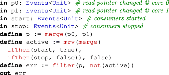
In order to evaluate our approach with TeSSLa_a specifications of some practical relevance, we took some specifications from the use case presented in Decker et al. (2017). Figure 8 shows the architecture of the use case: two physical cores running one thread producing data and multiple threads consuming data. The producer is writing to and the consumers are reading from a memory section shared between the two cores, which is organized as a ring buffer. The consumers are activated and deactivated by an external signal. For this system, the following three data race–related correctness properties are given in TeSSLa_a:

• (1) Starting and stopping the consumers work properly; i.e., the read pointer of the ring buffer is only modified if the consumers are currently active:

  

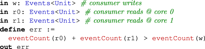
• (2) There are not more read operations than write operations; i.e., the sum of read operations performed by all consumers should be less than the sum of write operations performed by the producer:

  

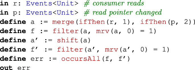
• (3) One entry in the ring buffer is not read twice; i.e, reading from the ring buffer and advancing the read pointer of the buffer must be an alternating event pattern:

  

Fig. 8

Overview of the ring buffer scenario from Decker et al. (2017)

4.2 Evaluation

With the empirical evaluation, we pursue to answer the following questions:

• (A) How well does the implementation exploit parallelism? The evaluation engine discussed in this paper uses a slight form of synchronization (essentially only the queues of events between nodes are added) that still guarantees a correct output. Hence, our implementation should be able to automatically utilize the parallel computational power of multiple cores.

• (B) How is the runtime influenced by the length of the input trace? The evaluation engine exchanges messages along the reversed dependency graph, which is acyclic. If the runtime of the computation nodes itself is constant per processed message, every additional input event should add a constant delta to the overall runtime.

• (C) What is the relation between the specification size and the runtime? Adding one extra computation node to the specification should add a constant delta to the runtime, because every event is now processed by one extra computational node.

• (D) What is the memory consumption of the implementation? In addition to the runtime, we are interested in the memory consumption in the scenarios described in the above questions, too.

To investigate these questions and evaluate the performance of our implementation, we measured the execution time and the memory consumption in relation to the number of processor cores, the length of the input trace, and the size of the specification. We took the specifications (1) to (3) presented in Section 4.1 as samples in order to derive specifications which cover all edge cases of practical specifications and can be varied in their size. Topologically, practical TeSSLa_a specifications are typically a variation and combination of long chains of computation nodes, tree-like structures distributing a single event to multiple computational nodes, and inverse trees combining and aggregating outputs of different computational nodes into a single verdict. Figure 9 shows the simplified dependency graphs of the specifications (1) to (3) presented in Section 4.1. The evaluation should only consider computation nodes, which store at most the previous input. Hence, the assumption of constant computation time per node is justified. Furthermore, we do not want to filter any events, and input values in the input events should not influence how the events are processed. Otherwise, adding more input events would not always have the same effect and the measurements would be biased.

Fig. 9

Simplified dependency graphs for the correctness properties (1), (2), and (3) and for the derived generalized chain scenario (4) and tree scenario (5)

Under these premises, we created two scenarios: the chain scenario and the tree scenario shown as (4) and (5) in Fig. 9. The chain scenario consists of a chain of abs functions. Every computation node directly depends on the output of the previous node. This is a worst case scenario in the sense that there are no two independent paths in the dependency graph, and each block sequentially depends on the previous node. The tree scenario goes one step further by first reusing the same input event multiple times repeatedly and then recombining all those by joining two inputs each in a logarithmic binary tree. This scenario has a maximal synchronization requirement, since the output node—the root of the tree—depends on all the intermediate computation nodes. One can observe from Fig. 9 that these two specifications are the two corner cases regarding interdependencies and hence required synchronization effort and thus can be seen as good representatives for practical TeSSLa_a specifications.

All benchmarks were performed on the same machine with up to 12 cores and 32 GB of RAM. The results displayed in Fig. 10 and Tables 1, 2, and 3 summarize the average of 20 runs. In addition to the overall runtime, the tables show the number of outliers ignored in the average, the error—i.e., the maximal deviation of the individual executions from the average—and the relative runtime per event or node, respectively.

• (A) Number of cores. For this benchmark, we used the chain specification with 16 nodes and the tree specification with 48 nodes. The input trace contains exactly 10,000 events. The results in Fig. 1 and the left plot in the first row of Fig. 10 shows that the execution time decreases drastically with an increase on the number of cores available, suggesting that our implementation is able to make an effective use of parallelism, even in the case of the completely linear dependency graph. The answer to question (A) is that our asynchronous implementation is able to exploit parallelism automatically in a pipeline fashion. Even though it is intuitively clear that independent nodes of the dependency graph can be executed in parallel, these results indicate that our implementation is also able to effectively exploit the potential parallelism when a chain of operators that are linearly dependent operate on different input events, by scheduling the corresponding nodes as actors as an asynchronous pipeline.

• (B) Number of events in the input. To study the dependency of the execution time with the input length, we reused the same specifications and modified the input sizes. The results are shown in Fig. 2 and the left plot of the second row of Fig. 10. The plots in cyan and magenta show the average time per event. With an increase on the input length, the static overhead is quickly amortized and the length of the trace becomes less relevant for the average event time. Consequently, in both cases, the relative time shows a decay towards a constant as more events are added.

• (C) Number of nodes in the specification. The execution time also grows more or less linearly in the size of the specification for both specifications. For this benchmark, we used input traces of 1000 events and increased the number of computation nodes in both specifications. The results are shown in Fig. 3 and the left plot of the bottom row of Fig. 10. Again, the relative time per event depicted in cyan and magenta shows a decay as more nodes are added, because the static overhead becomes less relevant. Even with the number of computation nodes now being exactly the same in the chain and the tree specification, the runtime for the tree specification is slightly higher. The tree specification has many more edges between the computation nodes than the chain specification and hence the message passing overhead is higher in this benchmark.

• (D) Memory consumption. Next to the runtime, Tables 1, 2, and 3 contain the memory usage, too. In Fig. 10, the memory consumption is shown in the corresponding plots on the right side. One can clearly see that increasing the number of used cores increases the memory usage. Since every computational nodes is realized as an actor in Elixir and every actor is equipped with a queue for every input, the number of actors and the number of queues are independent of the number of cores. The number of used cores influences the memory usage anyhow, because the Erlang virtual machine has to start threads on the cores and manage the communication between the different cores. One can further see that the number of input events influences the memory consumption due to the unbound queues in the actors: Since the input events are read from an input file, new events are incoming faster than they are processed in this setting and an increasing number of events are stored in the queues. Finally, memory consumption is influenced by the number of nodes in the specification since every node in the specification corresponds to a computational node equipped with input queues.

Fig. 10

Benchmarks. The plots on the left show the runtime and the plots on the right show the memory consumption. The blue/cyan lines with circle/triangle marks indicate the runtime of the chain specification and the red/magenta lines with square/diamond marks indicate the runtime of the tree specification. The blue/red lines show total values with labels on the left side of the plot. The cyan/magenta lines show relative values per event or node, resp. with labels on the right side of the plots

Table 1 Benchmarking the chain specification with 16 nodes (left) and the tree specification with 48 nodes (right), both with 10 ,000 input events and a varying number of cores. Average runtime of 20 executions without the outliers, error being the maximal deviation of the individual executions from the average

Table 2 Benchmarking the chain specification with 16 nodes (left) and the tree specification with 48 nodes (right), both with 12 cores and a varying number of input events. Average runtime of 20 executions without the outliers, error being the maximal deviation of the individual executions from the average

Table 3 Benchmarking the chain specification (left) and the tree specification (right), both with 10, 000 input events, 12 cores, and a varying number of nodes in the specification. Average runtime of 20 executions without the outliers, error being the maximal deviation of the individual executions from the average

Even though measurements can never fully cover all arbitrary TeSSLa_a specifications, these measurements have been chosen to represent extreme cases of the dependencies between computational nodes. Our empirical evaluation supports the feasibility of our distributed asynchronous monitoring approach in terms of efficiency.

4.3 Instrumentation and tool chain

As mentioned in Section 1, TeSSLa_a is designed to simplify FPGA-based implementations of the evaluation engine. Additionally, we also implemented auxiliary tools to use TeSSLa_a for the runtime verification of C programs, like a simple software instrumentation tool realized as a compiler pass of the LLVM Compiler Infrastructure. We added the TeSSLa_a functions function_call and function_return which generate an input stream with an event every time the function is called or returns, respectively, during the run of the program. This additional TeSSLa_a functions are pre-processed into a list of functions that need to be instrumented and replaced with input streams for further processing of the specification. This leads to the following tool chain from a TeSSLa_a specification φ:

• 1. Process φ into dependency graph G and identify the functions to instrument.

• 2. Compile the C code to LLVM IR code.

• 3. Instrument the LLVM IR code and compile the result to an executable.

• 4. Run the executable, which generates the input trace r.

• 5. Run the TeSSLa_a evaluation engine with G and r as inputs.

Steps 4 and 5 can be executed concurrently in tandem (online monitoring where the trace is processed while being generated) or running step 4 first, dumping the trace r to storage, and step 5 afterwords using the dumped stored trace as input.

This tool chain using the TeSSLa_a evaluation engine analyzed in this paper is available as an Atom plugin integrating all the steps described above. The plugin for the Atom editor is shown in Fig. 11. Other TeSSLa implementations not restricted to the acyclic TeSSLa_a fragment are discussed in Convent et al. (2018) and are available on the TeSSLa website.⁵

Fig. 11

Atom plugin for TeSSLa_a-based runtime verification of C programs. More information on the Atom plugin are available at https://www.tessla.io/acyclic/

5 Conclusion

We studied in this paper the problem of efficiently monitoring stream runtime verification specifications of real-time events and signals. In particular, our goal was to support the arrival of events at different speeds of input event streams and with different and varying latencies. The language we support in our solution is TeSSLa_a, an acyclic fragment of the stream-based runtime verification language TeSSLa for non-synchronized streams of piece-wise constant real-time signals. We introduced the notion of evaluation engines as an abstraction of online monitors that can execute asynchronously, based on independent building blocks that communicate using message passing. The main result is that, assuming a few local properties in each of the concurrent nodes (output completeness and progress), all executions for a given input compute an equivalent output. The possible differences between the outputs are in terms of the relative order of the output produced, but not in terms of the streams they compute. A novel notion of asynchronous transducers allows to formalize these equivalences, both for terminating and unbounded executions.

We then defined the operational semantics of TeSSLa_a in terms of evaluation engines. To achieve output completeness, we introduce the notion of progress events that allows the explicit communication of the absence of events in a given stream. Our results enable different evaluation engines, including asynchronous evaluation engines based on actors—which allow to exploit multi-core parallelism—and evaluation engines implemented in FPGAs which enable the utilization of massive hardware parallelism. Finally, we report in this paper an implementation of an evaluation engine written in Elixir/Erlang. Future work includes the extension of the approach to support richer specification languages, as well as supporting input streams that contain missing or approximate information or errors in their values or precise timings.

References

Agha, G. (1986). Actors: a model of concurrent computation in distributed systems. Cambridge: MIT Press.
Alur, R., Feder, T., & Henzinger, T.A. (1996). The benefits of relaxing punctuality. Journal of the ACM.
Asarin, E., Caspi, P., & Maler, O. (2002). Timed regular expressions. Journal of the ACM, 49(2), 172–206.
Barringer, H., Goldberg, A., Havelund, K., & Sen, K. (2004). Rule-based runtime verification. In Proc. of VMCAI’04, LNCS 2937 (pp. 44–57): Springer.
Bartocci, E., & Falcone, Y. (Eds.). (2018). Lectures on runtime verification - introductory and advanced topics, LNCS, Vol. 10457. Berlin: Springer.
Bauer, A., Leucker, M., & Schallhart, C. (2011). Runtime verification for LTL and TLTL. ACM Transactions on Software Engineering and Methodology, 20(4), 14.
Bauer, A., Küster, J. C., & Vegliach, G. (2013). From propositional to first-order monitoring. In Proc. of RV’13, LNCS, (Vol. 8174 pp. 59–75): Springer.
Baumeister, J., Finkbeiner, B., Schwenger, M., & Torfah, H. (2019). Fpga stream-monitoring of real-time properties. In EMSOFT. ACM.
Berry, G. (2000). Proof, language, and interaction: essays in honour of Robin Milner, chap. The foundations of Esterel, (pp. 425–454). Cambridge: MIT Press.
Bozelli, L., & Sánchez, C. (2014). Foundations of Boolean stream runtime verification. In In Proc. RV’14, LNCS, (Vol. 8734 pp. 64–79): Springer.
Caspi, P., & Pouzet, M. (1996). Synchronous Kahn Networks. In Proc. of ICFP’96 (pp. 226–238): ACM Press.
Chase, C.M., & Garg, V.K. (1998). Detection of global predicates: techniques and their limitations. Distributed Computing, 11(4), 191–201.
Convent, L., Hungerecker, S., Leucker, M., Scheffel, T., Schmitz, M., & Thoma, D. (2018). Tessla: temporal stream-based specification language. In Formal methods: foundations and applications - 21th Brazilian symposium, SBMF 2018, Recife, Brazil, November 26 - November 30, 2018. Proceedings lecture notes in computer science: Springer.
Cristian, F., & Fetzer, C. (1999). The timed asynchronous distributed system model. IEEE Transactions on Parallel and Distributed Systems, 10(6), 642–657.
D’Angelo, B., Sankaranarayanan, S., Sánchez, C., Robinson, W., Finkbeiner, B., Sipma, H.B., Mehrotra, S., & Manna, Z. (2005). LOLA: runtime monitoring of synchronous systems. In Proc. of TIME’05 (pp. 166–174): IEEE.
Decker, N., Gottschling, P., Hochberger, C., Leucker, M., Scheffel, T., Schmitz, M., & Weiss, A. (2017). Rapidly adjustable non-intrusive online monitoring for multi-core systems. In 20th Brazilian symposium on formal methods (SBMF 2017): Springer.
Decker, N., Dreyer, B., Gottschling, P., Hochberger, C., Lange, A., Leucker, M., Scheffel, T., Wegener, S., & Weiss, A. (2018). Online analysis of debug trace data for embedded systems. In DATE: IEEE.
Donzé, A., Maler, O., Bartocci, E., Nickovic, D., Grosu, R., & Smolka, S.A. (2012). On temporal logic and signal processing. In In Proc. of ATVA’12, LNCS, (Vol. 7561 pp. 92–106): Springer.
Eisner, C., Fisman, D., Havlicek, J., Lustig, Y., McIsaac, A., & Campenhout, D.V. (2003). Reasoning with temporal logic on truncated paths. In Proc. of CAV’03, LNCS 2725, (Vol. 2725 pp. 27–39): Springer.
Eliot, C., & Hudak, P. (1997). Functional reactive animation. In Proc. of ICFP’07 (pp. 163–173): ACM.
Faymonville, P., Finkbeiner, B., Schirmer, S., & Torfah, H. (2016). A stream-based specification language for network monitoring. In Proc. of the 16th Int’l conf. on runtime verification (RV’16), LNCS, (Vol. 10012 pp. 152–168): Springer, DOI https://doi.org/10.1007/978-3-319-46982-9_10.
Faymonville, P., Finkbeiner, B., Schledjewski, M., Schwenger, M., Stenger, M., Tentrup, L., & Hazem, T. (2019). StreamLAB: stream-based monitoring of cyber-physical systems. In Proc. of the 31st Int’l conf. on computer-aided verification (CAV’19), LNCS, (Vol. 11561 pp. 421–431): Springer.
Gautier, T., Le Guernic, P., & Besnard, L. (1987). SIGNAL: a declarative language for synchronous programming of real-time systems. In Proc. of FPCA’87, LNCS 274 (pp. 257–277): Springer.
Goodloe, A.E., & Pike, L. (2010). Monitoring distributed real-time systems: a survey and future directions. Tech. rep., NASA Langley Research Center.
Gorostiaga, F., & Sánchez, C. (2018). Striver: Stream runtime verification for real-time event-streams. In Proc. of the 18th int’l conf on runtime verification (RV’18), LNCS, (Vol. 11237 pp. 282–298): Springer.
Halbwachs, N., Caspi, P., Pilaud, D., & Plaice, J. (1987). Lustre: a declarative language for programming synchronous systems. In Proc. of POPL’87 (pp. 178–188): ACM Press.
Havelund, K., & Goldberg, A. (2005). Verify your runs. In Proc. of VSTTE’05, LNCS 4171 (pp. 374–383): Springer.
Havelund, K., & Roşu, G. (2002). Synthesizing monitors for safety properties. In Proc. of TACAS’02, LNCS 2280 (pp. 342–356): Springer.
Hewitt, C., Bishop, P., & Steiger, R. (1973). A universal modular ACTOR formalism for artificial intelligence. IJCAI, 235–245.
Jaksic, S., Bartocci, E., Grosu, R., Kloibhofer, R., Nguyen, T., & Nickovic, D. (2015). From signal temporal logic to FPGA monitors. In Proc. of MEMOCODE 2015 (pp. 218–227).
Jaksic, S., Bartocci, E., Grosu, R., & Nickovic, D. (2016). Quantitative monitoring of STL with edit distance. In Prov. of RV’16, LNCS, (Vol. 10012 pp. 201–218).
Leucker, M. (2011). Teaching runtime verification. In Proc. of RV’11, no. 7186 in LNCS (pp. 34–48): Springer.
Leucker, M., & Schallhart, C. (2009). A brief account of runtime verification. J. Logic Algebr. Progr., 78(5), 293–303.
Leucker, M., Sánchez, C., Scheffel, T., Schmitz, M., & Schramm, A. (2018). TeSSLa: runtime verification of non-synchronized real-time streams. In Proc. of the 33rd symposium on applied computing (SAC’18): ACM.
Maler, O., & Nickovic, D. (2004). Monitoring temporal properties of continuous signals. In FTRTFT (pp. 152–166).
Manna, Z., & Pnueli, A. (1995). Temporal verification of reactive systems: safety. New York: Springer.
Pike, L., Goodloe, A., Morisset, R., & Niller, S. (2010). Copilot: a hard real-time runtime monitor. In Proc. of RV’10, LNCS 6418: Springer.
Pnueli, A., & Zaks, A. (2006). PSL model checking and run-time verification via testers. In Proc. of FM’06, LNCS 4085 (pp. 573–586): Springer.
Reinbacher, T., Rozier, K.Y., & Schumann, J. (2014). Temporal-logic based runtime observer pairs for system health management of real-time systems. In Proc. of the 20th Int’l conf. on tools and algorithms for the construction and analysis of systems (TACAS’14), no. 8413 in LNCS (pp. 357–372): Springer.
Roşu, G., & Havelund, K. (2005). Rewriting-based techniques for runtime verification. Automated Software Engineering, 12(2), 151–197.
Sánchez, C. (2018). Online and offline stream runtime verification of synchronous systems. In Proc. of the 18th Int’l conf. on runtime verification (RV’18), LNCS, (Vol. 11237 pp. 138–163): Springer.
Selyunin, K., Nguyen, T., Bartocci, E., & Grosu, R. (2016). Applying runtime monitoring for automotive electronic development. In Proc. of RV’16, LNCS, (Vol. 10012 pp. 462–469).
Selyunin, K., Jaksic, S., Nguyen, T., Reidl, C., Hafner, U., Bartocci, E., Nickovic, D., & Grosu, R. (2017). Runtime monitoring with recovery of the sent communication protocol. In Proc. of CAV’17, LNCS, (Vol. 10426 pp. 336–355): Springer.
Sen, K., & Roşu, G. (2003). Generating optimal monitors for extended regular expressions. ENTCS, 89(2), 226–245.
Acknowledgments
We thank Jannis Harder and Sebastian Hungerecker for their work on TeSSLa and its compiler.
Funding
This work was funded in part by the BMBF project ARAMIS II with funding ID 01 IS 16025, the EU H2020 project COEMS under no. 732016, the EU H2020 project Elastest under no. 731535, the Madrid Regional Government under project “S2018/TCS-4339 (BLOQUES-CM)” and the Spanish National Project “BOSCO (PGC2018-102210-B-100)”.
Author information
Authors and Affiliations
Corresponding author
Additional information
Publisher’s note
Springer Nature remains neutral with regard to jurisdictional claims in published maps and institutional affiliations.
Rights and permissions
Open Access This article is licensed under a Creative Commons Attribution 4.0 International License, which permits use, sharing, adaptation, distribution and reproduction in any medium or format, as long as you give appropriate credit to the original author(s) and the source, provide a link to the Creative Commons licence, and indicate if changes were made. The images or other third party material in this article are included in the article's Creative Commons licence, unless indicated otherwise in a credit line to the material. If material is not included in the article's Creative Commons licence and your intended use is not permitted by statutory regulation or exceeds the permitted use, you will need to obtain permission directly from the copyright holder. To view a copy of this licence, visit http://creativecommons.org/licenses/by/4.0/.
About this article
Cite this article
Leucker, M., Sánchez, C., Scheffel, T. et al. Runtime verification of real-time event streams under non-synchronized arrival. Software Qual J 28, 745–787 (2020). https://doi.org/10.1007/s11219-019-09493-y
Published:
Issue Date:
DOI: https://doi.org/10.1007/s11219-019-09493-y