
Abstract
The coronal magnetic field is the primary driver of solar dynamic events. Linear and circular polarization signals of certain infrared coronal emission lines contain information about the magnetic field, and to access this information either a forward or an inversion method must be used. We study three coronal magnetic configurations that are applicable to polar-crown filament cavities by doing forward calculations to produce synthetic polarization data. We analyze these forward data to determine the distinguishing characteristics of each model. We conclude that it is possible to distinguish between cylindrical flux ropes, spheromak flux ropes, and sheared arcades using coronal polarization measurements. If one of these models is found to be consistent with observational measurements, it will mean positive identification of the magnetic morphology that surrounds certain quiescent filaments, which will lead to a better understanding of how they form and why they erupt.
1 Introduction
To understand coronal evolution and predict dynamic events such as coronal mass ejections (CMEs) and solar flares, we need to measure the coronal magnetic field. However, this is no trivial task. Much of the difficulty is due to the optically thin nature of the coronal plasma and the relatively weak intensities of coronal emission lines. Measuring the field will resolve many long-standing debates about the corona, including the magnetic-field morphology surrounding prominences.
Prominences can be extremely stable on the solar surface; some polar-crown filaments survive for many rotations (Gibson et al. 2006), but they are also known to erupt suddenly. When prominences are seen on the limb and are aligned with an observer’s line-of-sight (LOS), they are often seen to be embedded in coronal cavities. These cavities are typically depleted in density by a factor of about two relative to the surrounding streamer (Fuller and Gibson 2009; Schmit and Gibson 2011). Cavities are the coronal manifestation of the magnetic system that also includes the filament channel and the prominence (Hudson et al. 1999; Gibson et al. 2006; Heinzel et al. 2008; Gibson et al. 2010). Because the cavity comprises the bulk of the system volume, the magnetic structure of the system can be determined from measurements of the cavity. The cavity–prominence structure is known to erupt bodily as a CME (Maričić et al. 2004; Régnier, Walsh, and Alexander 2011). The initiation of these eruptions depends critically on the magnetic field threading through, and around, the prominence.
Flux-rope models with magnetic field wrapped around a distinct axis, and sheared-arcade models without such an axis, have both been posited as possible morphologies of prominences and their surrounding magnetic field (see Mackay et al., 2010 and references therein). Flux-rope systems have also been explicitly compared with cavities (Low and Hundhausen 1995; Gibson et al. 2006; Dove et al. 2011). Both morphological models contain dipped field lines where mass can cool and condense into prominence material. Coronal polarization measurements could provide a means of distinguishing between these structures, which would lead to a better understanding of not only the quiescent nature of prominences and cavities, but would also help in understanding how they are formed, and how they destabilize and erupt. Our objective in this article is to determine the characteristic polarization signatures of these different models of prominence cavities.
In Section 2 we discuss the difficulties of measuring the coronal magnetic field and the specifics of the Stokes vector in the Fe xiii 1074.7 nm coronal emission line. Section 3 describes the forward calculations, followed by details of the three individual coronal models in Section 4. We analyze these synthetic forward-modeled observations and look for distinguishing features, which can be compared to solar observations of prominence–cavity systems to identify magnetic morphologies. We present these features in Section 5 and conclude with a discussion of our results in Section 6.
2 Measuring the Coronal Magnetic Field
There are several methods currently employed to determine the magnetic field in the corona. Given that the thermal conductivity along the field is higher than across the field, the bright loops seen in extreme ultra-violet (EUV) and X-ray images of the corona trace out magnetic field lines. Using EUV images, it is possible to follow these lines subject to projection effects (Aschwanden et al. 1999). However, this method does not produce a measure of the magnitude of the field, and full three-dimensional (3D) traces require tomographic inversions and/or stereoscopic methods, which can be tricky in the optically thin coronal plasma. Moreover, this technique only provides magnetic morphology information on specific bright loops, and not the full volume containing the magnetic field.
Measuring Faraday rotation along an LOS to a known radio source supplies information about the LOS magnetic field, if the plasma density is known. This technique has been used to study the corona (Patzold et al. 1987; Jensen 2007), but a limited number of sight lines exist along which this technique is valid. Gyroresonant emission in radio wavelengths is related to the total magnetic-field strength in the emitting region, but is limited to areas of strong magnetic field (> 200 Gauss) such as active regions (White and Kundu 1997), although instrumentation with a broader spectral range, such as the Frequency Agile Solar Radiotelescope (FASR: Bastian, 2005) would allow for more extensive application. Observation of modified bremsstrahlung emission in radio and microwave frequencies provides information on the LOS magnetic field in the corona on the disk. These measurements sample a thin layer in the lower corona/upper chromosphere, not in the full coronal volume (Gelfreikh 1994; Grebinskij et al. 2000). In some coronal emission lines, particularly in forbidden magnetic-dipole emission lines in the infrared, resonant scattering of anisotropic light in a magnetized plasma can produce polarized emission subject to the Hanle and the Zeeman effects. We now discuss the use of coronal emission-line polarization in more detail and further proceed to forward-modeling of this emission.
2.1 Coronal Stokes Vector
Charvin (1965) was one of the first to show that linear-polarization signals from forbidden coronal emission-line transitions could be used to determine the plane-of-sky (POS) magnetic-field direction. Harvey (1969) was the first to attempt to use circular polarization to measure the LOS magnetic-field strength. Compared with modern technology, early detectors of the coronal Stokes vector had significantly lower signal-to-noise ratios, coarser resolution, and required longer integration times, which in turn limited temporal resolution. One such early detector was the Coronal Emission Line Polarimeter (Querfeld 1977), which was a scanning photodiode polarimeter. A full-Sun measurement with this instrument would typically take about two hours and contain 1408 data points from 1.01R⊙ to 1.65R⊙ (Querfeld 1977; Arnaud and Newkirk 1987).
In the intervening 40 years, there has been steady progress in the field of coronal polarization. Today, there are two main coronal polarimeters currently in use: The first is the Optical Fiber-bundle Imaging Spectropolarimeter (OFIS) on the Solar Observatory for Limb Active Regions and Coronae (SOLARC) at Mt. Haleakala (Lin, Kuhn, and Coulter 2004). It generates 128 spectra from a 16×8 fiber optic array that subtends 5×2.5 arcminutes. It is capable of measuring full Stokes profiles at each of the 128 positions. This instrument has been used to successfully measure the linear-polarization strength and direction in the Fe xiii 1074.7 nm line, and to determine an LOS field strength from circular-polarization signals above an active region (Lin, Kuhn, and Coulter 2004; Liu and Lin 2008). The second instrument is the Coronal Multi-channel Polarimeter (CoMP: Tomczyk et al., 2008), which is installed at the Mauna Loa Solar Observatory, and began taking full-corona measurements in October 2010. CoMP is an imaging coronagraph polarimeter with a tunable birefringent filter capable of detecting the Fe xiii 1074.7 nm and 1079.8 nm lines as well as the He i 1083 nm line. The new CoMP observations provide, for the first time, daily full-Sun observations of the magnetic field in the corona. The primary observables of CoMP are the four Stokes parameters (I, Q, U, V).
These observations are taken above the solar limb in the corona, which is optically thin in these wavelengths, and thus the measurements contain information from an extended LOS source. The polarization signal strength is weaker than the line intensity (linear polarization/intensity \(\thickapprox10^{-2}\) and circular polarization/intensity \(\thickapprox10^{-4}\) for a one-Gauss field: Arnaud and Newkirk, 1987; Lin, Penn, and Tomczyk, 2000). It takes on the order of a few minutes to obtain a useable full-Sun linear-polarization measurement with CoMP, and circular-polarization measurements of sufficient signal-to-noise are made by averaging over an hour of data (Tomczyk et al. 2008). The polarization is the result of resonant scattering of anisotropic incident radiation by highly ionized coronal plasma in the presence of an external magnetic field. However, different aspects of this unified process dominate the linear- and circular-polarization signals of the coronal emission lines (e.g. Casini and Judge, 1999; Casini, 2002; Judge, 2007; Rachmeler, Casini, and Gibson, 2012, and references therein). We restrict the rest of this discussion to the Fe xiii 1074.7 nm coronal emission line. This is also the line used in the forward calculations.
The linear-polarization signal is completely dominated by the Hanle effect: a depolarization of scattered light associated with a radiation-induced population imbalance of the atomic levels (Trujillo Bueno 2001). The atomic alignment [σ] describes this population imbalance. The transverse Zeeman effect, which is due to the energy splitting of the magnetic sublevels by the coronal field, is a secondary source of linear polarization, because the splitting is smaller than the thermal width of these coronal lines (the transverse Zeeman effect is quadratic in the field strength). The Larmor frequency is higher than the inverse lifetime of the excited state, so the linear polarization signal occurs in the strong-field regime, also known as the saturated Hanle effect. In this regime, the linear-polarization strength and direction is dependent on the angle of the magnetic field, but no information about the magnitude is contained in the signal.
The strength of the total linear polarization [\(L=\sqrt{Q^{2}+U^{2}}\)] (same as P in Dove et al., 2011; Rachmeler, Casini, and Gibson, 2012) is dependent on the angle [Θ] between the LOS and the local magnetic-field vector. Specifically, L ∝ sin2Θ such that L is strong when the magnetic field is in the POS, and weak when the magnetic field is along the LOS. The relative strengths of Q and U are used to determine the azimuth angle [Ψ; U/Q=tan2Ψ], the POS angle of the LOS integrated magnetic field. There is a 90∘ ambiguity known as the Van Vleck effect (van Vleck 1925; House 1977) such that the magnetic-field direction could be parallel or perpendicular to the measured Ψ. When the local magnetic field is at the Van Vleck angle of roughly 54.7∘ with respect to solar radial, the light becomes unpolarized, and the strength of L goes to zero. When the magnetic field is less than 54.7∘ from radial, Ψ is parallel to the direction of the POS component of B, but switches to perpendicular when that angle is surpassed (see, e.g., Figure 5(c)). The Van Vleck effect results in linear polarization directions in the corona that are mostly radial (Arnaud and Newkirk 1987). If the location of the Van Vleck inversion can be identified, the 90∘ ambiguity can be removed, although a 180∘ ambiguity remains.
A measure of the magnetic-field strength is not possible with linear polarization in this regime, but the circular polarization does contain information about its magnitude along the LOS. The Stokes-V profile is proportional to BcosΘ. The longitudinal Zeeman effect (which is linear in the field strength) is the main contributor to the circular-polarization signal. However, the atomic alignment can yield a significant correction to this signal, changing the amplitude of the anti-symmetric V profile, and therefore affecting the diagnostics of the magnetic-field strength (Casini and Judge 1999).
Stokes I, Q, U, and V are all dependent on the plasma parameters in the emitting region. They are weakly dependent on the temperature as long as the emission line is excited. All Stokes components are directly weighted by the density. At a given location along the LOS, the density dependence cancels when analyzing the relative polarizations [L/I and V/I], but this is not the case in a signal that is integrated along the LOS. For an integrated measurement, the signal will be dominated by the areas along the LOS that have the highest density. Since collisions tend to equalize the sublevel populations, a density dependence also enters into the Stokes vector through σ.
There are two general methods for interpreting the coronal-polarization measurements. The first is by inverting the signals into physical properties of the magnetic field. This is the approach taken with photospheric polarization data. However, because the plasma is optically thin in the corona, the signal is coming from an elongated source along an LOS. Inversions generally solve for a single point of emission, so not all calculations will converge to a solution. Inversions of these polarization signals require numerous initial assumptions about the emitting plasma, and are quite difficult due to multiple integrals that must be inverted. These calculations are known to be ill-posed (Judge 2007). Information about atomic level-populations, and hence the plasma parameters, at each point along the LOS is required to solve the POS magnetic-field direction. To determine the field strength and direction everywhere, tomographic inversions are needed. The tomographic inversion process requires multiple viewpoints of the field, and if only one is available, as is currently the case, solar rotation must be used to generate these viewpoints (Kramar, Inhester, and Solanki 2006; Kramar and Inhester 2007). This adds the additional assumption that the coronal field does not change appreciably over rotational timescales. An alternate approach to extracting information from coronal-polarization data is forward-modeling.
Our forward technique involves creating simulated polarimetric observables from models of the corona (Judge and Casini 2001; Judge, Low, and Casini 2006). In the work presented here, we use this technique to study the differences between several pre-CME magnetic morphologies, and expand upon the work begun by Judge, Low, and Casini (2006). The ultimate goal of this research is to determine if it is possible to use coronal polarization to positively identify flux ropes, or other magnetic morphologies, in the cavities that surround pre-CME filaments.
3 Description of the Forward Calculations
The basic procedure of our forward technique is to calculate the Stokes vector produced along a given LOS in a magnetic model and build an image from a grid of sight lines. To do this, the magnetic field, temperature, density, and velocity at every location along each LOS are used. Given this information, we calculate the level populations and the emitted polarization profiles for the Fe xiii 1074.7 nm transition at each location using the publicly available Fortran code (FORCOMP) discussed by Judge and Casini (2001). The forward model has an IDL user interface and is publicly available for download and use ( people.hao.ucar.edu/sgibson/FORWARD/ ).
FORCOMP first calculates the statistical-equilibrium equations based on the location and the local plasma parameters from the model: height above the solar surface [h], density [ρ], temperature [T], magnetic field [B], and velocity [v]. Using standard atomic data, the statistical-equilibrium equations determine the relevant level populations of the atomic system for the transition in question. The code treats inelastic and superelastic collisional processes, but neglects elastic collisions. This omission affects the magnitude, but not the direction, of L and leads to a small uncertainty in V. The LOS field strength and the POS field direction are not strongly affected by the elastic collisions. Once the level populations are determined, FORCOMP solves the radiative-transfer equations to calculate the polarization of the reemitted radiation in the direction of the observer (Judge and Casini 2001). The signals are then integrated over wavelength into a single number for each pixel (or LOS), and are assembled into an image.
The benefit of the forward technique is that we can easily calculate the simulated polarization signals from a theoretical model of a magnetic system and then compare these images with observations. It allows us to test the theories against an observable that is directly sensitive to the magnetic field in the corona. Additionally, it allows for comparison between the models themselves.
The forward-model outputs Stokes I, Q, U, V and combinations thereof. We use mainly intensity [I], relative linear polarization [L/I], azimuth [Ψ], and relative circular polarization [V/I].
4 MHD Models
For our study of magnetic flux rope and sheared-arcade signatures in the corona, we used three models, each having a distinct magnetic morphology: The first model is a 3D analytic spheromak flux rope in exact equilibrium (Gibson and Low 1998, 2000). The second is an azimuthally symmetric (2.5D) cylindrical flux rope taken from an MHD simulation created to study current-sheet formation during CME initiation (Fan and Gibson 2006). The last is a 2.5D sheared arcade taken from MHD simulations of CME initiation by the multipolar breakout mechanism (Antiochos, DeVore, and Klimchuk, 1999; Karpen, Antiochos, and DeVore, 2012, and references therein). All models are in, or near, equilibrium and have been argued as models for prominence magnetic structure. The two flux-rope models contain a region of concave-up magnetic dips that can support prominence plasma against gravity, and they also capture many observed properties of coronal cavities (Hudson et al. 1999; Gibson and Low 2000; Mackay et al. 2010; Reeves et al. 2012). Sheared arcades in 2.5D typically contain only concave-down regions that can support time-dependent prominence condensations if the field is sufficiently flat (Karpen et al. 2001). In three dimensions, sheared arcades can develop regions of concave-up field lines like those in flux ropes, and they then can support the plasma statically against gravity (Antiochos, Dahlburg, and Klimchuk, 1994; Luna, Karpen, and DeVore, 2012, and references therein).
We used a single snapshot from the two time-dependent MHD models. Because we are studying the steady-state pre-CME magnetic structure, all velocities were set to zero. The times used are those where the field is near equilibrium, and thus have close to zero velocity everywhere.
Two of our models are 2.5D. Azimuthal symmetry creates structures that are elongated along the LOS. When structures are highly 3D, the magnetic information can become smeared along the LOS, making magnetic signatures more difficult to identify. We used 2.5D models because the observational signatures of the magnetic field we are studying are clear coronal cavities. When a coronal filament channel and associated neutral line are along the LOS – nearly parallel with the solar Equator – a cavity commonly becomes visible, which implies that cavities are elongated along the LOS (Gibson et al. 2010). The 2.5D assumption is thus justified by cavity observations.
For the spheromak model, we used the density and temperature provided by the analytic model. The parameters were chosen such that the density and temperature vary only slightly in the calculation domain (Dove et al. 2011). For the two MHD models, a range of plasma parameters was explored. The goal of this work is to study the impact of the magnetic morphology on the polarization signatures. We looked at our models both with the original plasma distributions from the MHD simulations and with simple spherically symmetric plasma profiles. These new plasma distributions are not strictly in equilibrium with the magnetic fields. However, they serve the useful purpose of providing a means of distinguishing the features in the polarization data that are caused by the magnetic morphology from those that are heavily influenced by the plasma parameters. In addition, any effects of changing the plasma distributions on the magnetic-field structures would be very weak, since the prominence and cavity are in the low-β regime and are nearly in force-free equilibrium in both MHD examples.
Coronal Stokes vectors were calculated for each theoretical system using the forward code described in Section 3. We compared these polarization signatures with each other to determine their similarities and differences and to identify their distinguishing features.
4.1 Model Descriptions
The first magnetic system we explored is that of an analytic spheromak flux rope. A more detailed study of forward-model results from this particular flux rope can be found in Dove et al. (2011). The spheromak model (Figure 1) is an exact solution to the MHD equations in full magnetostatic equilibrium (Gibson and Low 1998). The magnetic field of the flux rope is a closed, twisted-flux system attached to the photosphere, which has been shown to reproduce observational features of a three-part CME including the cavity and the bright prominence (Gibson and Low 2000). The external field has a split bipolar configuration with a hydrostatic density background. We used an orientation such that the flux-rope axis, and hence the prominence material, is oriented along the LOS, and the axial magnetic field is directed toward the observer (Figure 1(b)). As stated by Dove et al. (2011), we chose a parameter set such that the density is close to spherically symmetric. The background-density profile was taken from Schmit and Gibson (2011). The density decreases from around 5×108 cm−3 at photosphere to about 3×107 cm−3 near the top of the spheromak at 1.3R⊙. The temperature is between 7×10⁵ and 1×10⁶ K. The magnetic-field strength is strongest at the axis, where it is around 1 G, and the external field strength near the flux rope is about 0.1 G. Thus, the plasma β is high outside the spheromak, above 100, and between 1 and 10 in most of the flux rope.

Field-line traces in the analytic spheromak flux-rope model seen from two different view points. Prominence material would theoretically sit below the thick black line, which traces the flux-rope axis, in the dips of the magnetic field. We used the orientation in b) in the forward calculations, with the magnetic field along the axis pointed toward the observer. An animated version of this figure is available in the electronic supplementary material.
The second model is a 2.5D axisymmetric cylindrical flux rope (Figure 2) and is described in Fan and Gibson (2006). This numerical model comprises a 2×10⁶ K isothermal atmosphere occupied by a potential arcade field under which a twisted toroidal flux tube kinematically emerges. With continual emergence, the system is quasi-static until time t=114R⊙/v A0, where v A0 is the characteristic Alfvén speed, after which the flux rope erupts. If the emergence is stopped before that, the system remains stable. We analyzed a time step at t=114 where the emergence was stopped at t=112. The model extended from 1R⊙ to 14.4R⊙ radially and from π/3 to 2π/3 in latitude. For the forward analysis, the system was oriented such that the flux rope was in the equatorial plane and the axial field pointed away from the observer. The magnetic-field strength at the axis was about 10 G. The electron density in the flux rope was on the order of 106−7 cm−3. The plasma β was below 0.1 except near the footprint of the arcade immediately surrounding the flux rope.

Field lines traced from the 2.5D axisymmetric cylindrical flux rope. Colors on the field lines represent the strength of the y-, or axial, component of the field. An animated version of this figure is available in the electronic supplementary material.
The third model (Figure 3) is a 2.5D axisymmetric numerical datacube of a breakout quadrupolar system (Karpen, Antiochos, and DeVore 2012). The computational domain extended from 1 to 125R⊙ radially and over π radians in latitude. The system was energized by shearing the innermost polarities near the neutral line. The shearing resulted in a field that is pointed away from the observer in our orientation. The field that connects these two polarities sheared and expanded both radially and laterally. Because a simple adiabatic energy equation and a closed lower-boundary condition were used, the plasma entrained in the sheared field rarefied and adiabatically cooled relative to the background. This configuration did not form a flux rope with a central axis until flare reconnection set in after the eruption. The time shown in Figure 3 is t=60 000 seconds; stopping the shearing motions at this time resulted in a stable equilibrium state, while continuing the motions led inexorably to an eruption. In and around the sheared arcade, the magnetic-field strength was about 1 G. In this same area, the plasma densities were 106−7 cm−3. The temperature reached a local minimum around 3×10⁵ K within the sheared field, while it was about 106 in the surrounding, unsheared field. The plasma β was below 0.01 in the sheared region and of order unity in the unsheared region (except, of course, in the immediate vicinity of the null point, where β becomes very high).

Field lines traced from the 2.5D sheared arcade model. Colors on the field lines represent the strength of the y-, or axial, component of the field. An animated version of this figure is available in the electronic supplementary material.
5 Results
Interpreting a polarization image is not necessarily straightforward (see Judge, 2007; Rachmeler, Casini, and Gibson, 2012 for detailed descriptions of the signal interpretation). For L/I images (i.e. Figure 4(b)), the magnitude of the signal is always positive, and the images are usually plotted on a logarithmic scale. Bright areas indicate magnetic field that is primarily in the POS. Dark areas generally indicate magnetic field that is along the LOS. Sharp, elongated dark structures are usually indicative of Van Vleck inversions, marking where the magnetic field is at an angle of ≈ 54∘ from radial. The L/I images may have the magnetic-field direction overlaid as arrows or lines. In the images presented in this article, the red arrows indicate the true POS direction of the magnetic field in a thin POS slice that bisects the Sun. The blue lines indicate the azimuth direction of the linear polarization, which is subject to the 90∘ Van Vleck ambiguity (Section 2.1). They are generally parallel when the magnetic field is close to radial, and perpendicular when it is not. V/I images are plotted on a linear scale with blue as negative and red as positive; white is zero. In our coordinate system, positive Stokes V (blue) indicates magnetic field toward the observer.

Forward-model results of the spheromak flux rope. a) Stokes intensity, b) relative linear polarization, c) relative linear polarization with magnetic-field direction plotted as red arrows and integrated polarization azimuth direction plotted as blue lines, d) relative circular polarization.
5.1 Spheromak Flux Rope
We used the parameter set from Dove et al. (2011) to demonstrate the main features for the spheromak flux rope. In the LOS-integrated images, the following features are identifiable and are robust signatures of this magnetic morphology: Figure 4 shows the forward-model results, as presented also in Dove et al. (2011). We summarize the conclusions from that analysis as follows:
-
i)
Dark L/I central core. A dark core is clearly visible at the location of the flux-rope axis in the L/I image (Figure 4(b); Z=0, Y=1.1). This is due to the LOS field associated with the axis. The axis of this type of flux rope is particularly clear because it is straight along the LOS, and not curved like the axis of the cylindrical flux rope. The dark central core is visible if the axis is oriented within about 30∘ of the LOS.
-
ii)
Dark L/I outer ring. A ring of darker L/I is visible at the edge of the spheromak bubble (Figure 4(b)), and it is also associated with LOS field. This ring is much fainter than the axis field because B on the outer edge of the bubble is only aligned with the LOS in a relatively narrow volume of space.
-
iii)
Bright L/I ring. Between i) and ii) is a bright ring in L/I (Figure 4(b)), which is due to the POS field in the flux rope.
-
iv)
Radial azimuth. The linear polarization direction shows no clear Van Vleck inversion locations (blue lines in Figure 4(c)). Although there are Van Vleck inversions within the spheromak, the rotation of the field along the LOS smears these out such that they are not visible in the integration.
-
v)
Bi-directional circular polarization (V/I). The circular polarization comprises a clear circular positive signal around the axis surrounded by a weaker rung of negative signal (Figure 4(d)). The presence of both positive and negative Stokes-V is not found in either of the other models studied here.
5.2 Cylindrical Flux Rope
Figure 5 shows the forward-model results for the cylindrical flux-rope configuration. To test the robustness of the magnetic signatures in the polarization signals, we ran the forward calculations on three cases. Case F1 used the original density and isothermal temperature of T=2×10⁶ K from the MHD model (Figure 5). Case F2 used an isothermal hydrostatic density fall-off with a scale height of \((2\mathrm{R}_{\odot}k_{b}T)/(G\mathrm{M}_{\odot}m_{p})\thickapprox 0.13\mathrm{R}_{\odot}\) [R⊙ and M⊙ are the solar radius and mass, k b is the Boltzmann constant, G is the universal gravity constant, m p is the mass of a proton, and T=1.5×10⁶ K is the temperature] and a density at the coronal base of 5.8×10⁸ electrons cm−3. Case F3 used a hydrostatic power-law density and temperature function derived from fits to coronal-streamer densities (Gibson et al. 1999). The magnetic field in this model was in nearly force-free equilibrium. The imposed plasma was also low-β. If re-relaxed to true equilibrium, the scale-height of the plasma along field lines would be altered, but the field topology would remain nearly unchanged.

Forward-model results from the flux-rope model case F1 with the density of the original MHD data cube and a temperature of 2×10⁶ K. a) Stokes intensity, b) relative linear polarization, c) relative linear polarization with magnetic-field direction plotted as red arrows and integrated polarization azimuth direction plotted as blue lines, d) relative circular polarization.
Stokes-I changed noticeably when a spherically symmetric density was used. Almost none of the structure seen in F1 (Figure 5(a)) is present in F2 or F3 (not shown). This is not surprising because the intensity of emitted radiation is strongly dependent on the local plasma density, so a spherically symmetric density results in a virtually spherically symmetric Stokes-I. The relative linear polarization signals varied little between the three cases (Figure 6); these differences are discussed at the end of this section. We first analyze the signatures of F1.
-
i)
Dark ∨-shaped Van Vleck inversions in the arcade. These are the Van Vleck inversions in the external arcade field (Figure 5(b); Y=1.4 to 2). The field outside of the ∨ is less than 54∘ from radial, and the field inside the ∨ is greater than that. This is clearly visible (Figure 5(c)) in the shift of the linear-polarization direction (blue lines) from parallel to perpendicular to the POS magnetic-field direction (red arrows). These two Van Vleck inversions extend downward into the flux rope.
-
ii)
Darker central region in L/I. In general, the region near the flux-rope axis (Z=0, Y=1.35) is slightly darker (Figure 5(b)). This is because there is more LOS field in this region, so the linear-polarization signal is lower. However, because of the LOS integration and the curvature of the central flux-rope axis, the location of the axis is unclear. See also iii) below.
-
iii)
Dark beads in L/I near the axis. These are visible in F1 and F3, but not in F2 (Figure 6). These locations are dark because they are signatures of the LOS field in the flux-rope axis. This flux rope is axisymmetric, so it curves around the limb of the Sun. The curvature results in a perspective effect such that the location of the LOS field is only co-spatial with the location of the flux-rope axis in the central POS slice. The true location of the flux-rope axis is not readily apparent in the integrated data because the volume of space where they are co-located is a small. The location of the LOS field follows a ⊃-shaped arc whose legs coincide with iv).
Figure 6 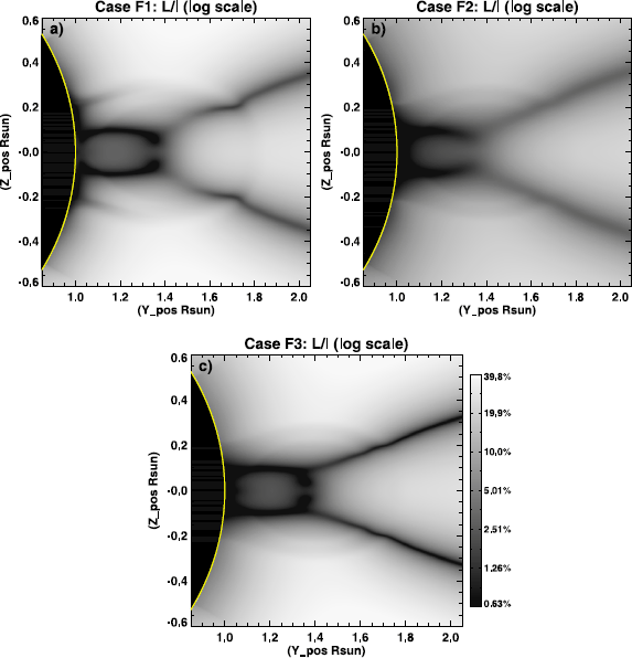
Comparison of the relative linear polarization for the three cases of the cylindrical flux rope. All three images use the same scale.
-
iv)
Two dark horizontal lines in L/I intersecting the photosphere. These are a combination of a Van Vleck inversion in the lower part of the flux rope and the LOS field from the legs of the ⊃-shape described in iii) and are thus the darkest features in the image.
-
v)
Slightly spoked azimuth direction. The azimuth directions are mostly radial, but there is a slight spoke-like signature around the flux-rope axis (Figure 5(c)). Since the Van Vleck inversion locations are obvious (in this model), the 90∘ ambiguity can be removed, and the flux-rope nature of the field becomes evident. Even without removing the ambiguity, the slight spoke may be a feature that can help to identify this type of magnetic morphology. Note that the linear-polarization azimuth direction (blue lines) everywhere is close to radial.
-
vi)
Bulb of circular polarization. The circular polarization has the same sign throughout (Figure 5(d)). The strongest signal comes from above the limb and surrounds the location of the flux-rope axis.

Although almost all these listed features are present in each case, some are more pronounced in certain cases. For instance, the dark beads in iii) are distinctly visible in F3, but not at all in F2. The density differences in each case change the weighting of the signal along the LOS. Thus, certain features are more or less clear depending on whether the signal is concentrated at the central POS, or spread out along the LOS. Case F2 has the most gradual density drop with height, and thus the dark beads from iii) are overcome by brighter signal in the foreground and background.
5.3 Sheared Arcade
Much like the cylindrical flux-rope model, we ran the forward calculations on the sheared-arcade model with several different density and temperature profiles. The cases presented here are as follows: S0 – the density and temperature provided by the MHD model; S2 – the density provided by the MHD model and isothermal temperature of 1.5×10⁶ K; S3 – hydrostatic streamer density and temperature fit from Gibson et al. (1999). We did not relax the configuration to equilibrium with the imposed plasma parameters. In all cases, the plasma was low-β except in the region of the null-line. We do not discuss the results from S0 because the temperature of the plasma falls below the minimum temperature threshold for the forward-calculations (around 5×10⁵ K). Most of the sheared-field plasma is at or below this temperature, due to the assumption of adiabatic energy transport, so any calculations on the original data only produce signal from the unsheared field, which is not useful for this work.
Figure 7(g), (h) shows the comparison of the integrated L/I for the S2 and S3 cases in the sheared region. We have looked at the polarization signals from thin POS slices along the LOS, and found that for any given slice, the L/I is qualitatively similar between the two cases. The differences seen in Figure 7 arise from the relative contributions to the integrated signal from the sheared field versus the background unsheared field. Stokes I, Q, and U are weighted by density. Hence, higher-density regions contribute more to the integrated signal than lower-density regions. The original density was used in S2 and a spherically symmetric density was used in S3. These densities are plotted in Figure 7(a), (b). Note that in S2, the density in the unsheared field is about an order of magnitude more dense than the sheared field because of the large volumetric expansion of the sheared field and the closed lower boundary condition imposed in the simulation. From a broad range of observations, it is known that streamers tend to be about a factor of two more dense than the embedded cavity (Fuller and Gibson 2009; Schmit and Gibson 2011). Thus, the S3 results emphasize the sheared field too much, and the S2 results emphasize this region to little compared with observations.

Forward-model results from the sheared arcade system. The left column shows case S2 and the right column shows case S3. a) and b) Density in the central region, the electron number density is given by 10X cm−3, where X is the value indicated by the color bar; c) and d) relative linear polarization of the entire system; e) and f) relative linear polarization of the central region; g) and h) same as above overlaid with red field vectors and blue azimuth directions; i) and j) relative circular polarization of the inner region.
The following list describes the features that are present in the data. After the list we analyze in more detail features that are found to a lesser degree or not at all in one of the cases.
-
i)
Quadrupolar Van Vleck signal. A clear Van Vleck signature is associated with the quadrupolar field (Figure 7(c), (d)). Even in the absence of any sheared field, there would be three pairs of Van Vleck inversions associated with the inner three loop systems. These pairs are the top two, the middle two, and the lower two elongated Van Vleck nulls.
-
ii)
∨-shaped Van Vleck inversion. At the top of the central loop system, there are Van Vleck lines in a ∨-shape (Figure 7(e), (f); at a height of 1.6 – 2R⊙), which is analogous to property i) in the cylindrical flux-rope model. The sheared field is confined to the central part of this system (i.e., the areas of negative V/I in Figure 7(i), (j)) and the ∨-shaped Van Vleck lines are associated with the unsheared portion of this central magnetic-loop system (dark-blue loops above the sheared field in Figure 3).
-
iii)
Parallel Van Vleck inversions. In the sheared field, there are two dark parallel Van Vleck inversion lines (Figure 7(e), (f); at a height of 1 – 1.6R⊙) that emanate from the photosphere and connect to the ∨-shape listed in ii). The parallel Van Vleck inversion lines are associated with the legs of the sheared region. This field is inclined toward/away from the observer at ≈ 54∘ from radial. These inversions are more pronounced in S3 than in S2.
-
iv)
Dark LOS core in L/I. The central sheared area generally has a lower linear polarization magnitude due to the presence of fields that are more LOS than the surrounding field. This effect is stronger in S3 than in S2.
-
v)
Anomalous LOS signal in L/I. A dark spot in L/I is visible in the sheared-field region in case S3 (Figure 7(f); Z=0, Y=1.35). This is not due to an axis of LOS field. This anomalous LOS signal (Rachmeler, Casini, and Gibson 2012) arises from cancellation in the LOS-integrated Stokes Q and U due to the symmetry in the system and is dependent on the relative density in the sheared and unsheared regions. This feature is not present in S2 (Figure 7(e)).
-
vi)
Non-radial azimuth direction. In the sheared-field region, the linear-polarization azimuth direction is parallel to the limb in the S3 case (blue lines in Figure 7(h)), which creates an illusion of a cylindrical flux rope. In this area the magnetic-field angle exceeds the Van Vleck angle, so the true field is perpendicular to the observed azimuth direction. Note that at this location, the field is actually predominantly in the LOS, and the POS component is weak. This feature is not present in S2 (Figure 7(g)).
-
vii)
Strongest circular polarization near limb (V/I). The relative circular polarization is shown in Figure 7(i), (j). The shear is not concentrated above the limb, as in the flux-rope case, but at the limb. The features within the negative V/I in S2 are due to density variations (Figure 7(a)). The V/I in the S3 case shows a smooth profile.
Most of these features are present in both cases, but they are not always obvious in the integrated S2 data. The locations of the Van Vleck inversion and the LOS field i) – iii) are the same in both cases. Figure 8 shows the LOS integrated values of Stokes Q and U [\(L=\sqrt{Q^{2}+U^{2}}\)] for cases S2 and S3. The locations of lowest Q and U are the same for both cases, but there are no true nulls in Q inside the sheared-field region in S2. Thus, the integrated L/I for S2 (Figure 7(e)) does not show true Van Vleck nulls. The inversions are there, but the signal from the unsheared portion of the LOS obscures them.

Integrated Stokes Q and U signals from cases S2 and S3 of the sheared-arcade model. Lines of zero Q or U are shown in magenta.
There is clearly no anomalous LOS signal iv) in S2 (Figure 7(e)). This is because the background dominates the integrated signal at all heights in this case. Investigation of the polarization generated in thin POS slices shows that the unsheared field in all cases produces a negative Stokes-Q signal, and the sheared field produces a signal that is predominantly positive. The relative density in the sheared and background field determines where the sheared field dominates in the integrated Stokes profiles. The integrated Stokes-Q signal for S3 (Figure 8(b)) is positive in the central region, showing that the sheared field dominates the LOS signal there. Where a zero-line in Stokes Q crosses a zero-line in Stokes U (Figure 8(b), (d)) there is an anomalous LOS signal (Figure 7(f)) (Rachmeler, Casini, and Gibson 2012). Since the sheared field in S2 has a lower density, the integrated Stokes Q is always dominated by the background field (Figure 8(a)) and is never negative. Thus there is no anomalous LOS signal in S2.
The relative weighting of the sheared versus the unsheared field also causes the difference in the azimuth direction for cases S2 and S3. The volume of space that contains a sheared field lies inside a Van Vleck inversion – such that the azimuth is perpendicular to the POS magnetic-field direction – and inspections of a thin POS slice reveals azimuth directions that are consistent with Figure 7(h). The integrated L/I in case S2 shows radial azimuths because the background field dominates, so the non-radial azimuth signal is overwhelmed.
6 Discussion
We have presented three coronal models and their synthetic polarization signatures. We found that each of these models is distinct and distinguishable, even when using linear polarization alone. The spheromak flux rope is the most recognizably different, while the cylindrical flux rope and the sheared-arcade models are somewhat similar.
This work highlights the importance of using a forward approach on coronal emission-line polarization. It can teach us what to look for in observations, such as Van Vleck inversions and LOS field. It also calls attention to the fact that we cannot trust our intuition to pick out magnetic morphologies. The sheared-arcade model is a good example of this. On initial inspection, the polarization signatures of the S3 sheared arcade resemble a flux rope; the azimuth direction is parallel to the limb between the inner Van Vleck inversions, and a false axial signature may be present. Both of these signatures can be logically explained when analyzing the forward results, but this example underlines the need for forward or inverse analysis before magnetic-structure identification can be made. Another important strength of the forward approach is that it fully takes into account the LOS integration of the polarization signal. The optically thin plasma is a significant challenge for the inverse technique and so is often seen as a limitation for coronal polarization data as a whole, but the forward approach incorporates the lack of opacity. By looking at a given magnetic configuration with multiple plasma profiles, we can also learn about how the signatures change due to the plasma parameters alone. We have shown that for cavities that are about half as dense as the surrounding streamer, the polarization signature from the streamer can obscure some of the features that are present in the cavity. For future observations, it is clear that knowledge of the LOS density structures is important for analysis and interpretation. Density diagnostics that determine a 3D density distribution could be used in conjunction with polarization observations and forward calculations.
Our work is not the first to use this forward approach to understand hypothetical or actual observations. Judge, Low, and Casini (2006) applied the same forward code to study prominence-supporting magnetic fields and current sheets. Liu and Lin (2008) compared observations of an active region on the limb with potential-field extrapolations to study how the LOS affects the fit of the forward calculation to the observations. Dove et al. (2011) compared the spheromak model presented here with an early CoMP observation of a large cavity. The next important step is to take the knowledge gained with these forward studies and apply it directly to observations, looking for the specific morphologies; this work is already underway. Baķ-Stȩślicka et al. (2013) have found that cavities observed in CoMP in 2011 and 2012 usually have a characteristic “rabbit-head” signature in L/I. This signature consists of two Van Vleck inversions, with or without a dark central region indicating an LOS field. They have shown that this observation is consistent with a 3D flux-rope topology where the height of the dark central “head” is approximately co-spatial with the center of the cavity.
Observations carry their own challenges because of noise and small-scale density structures in the corona. CoMP is an occulted coronagraph and the occulter is at approximately 1.05R⊙, which means that especially for small cavities, the distinguishing characteristics such as azimuth direction would most likely be obscured by the occulter. We used extremely simplified density structures to isolate the magnetic features, but in reality, the Stokes-I observations are highly structured. By analyzing relative linear and circular polarization, we removed some of the density component, but the signal is still density dependent, and we showed that the relative importance of the structures along the LOS is highly dependent on their density. Our current approach is more applicable in coronal cavities, which are, in general, fairly smooth in intensity compared with active regions with clear bright loops. In future forward-modeling research, more realistic density models are needed. The observational noise, the occulter, and the highly structured coronal density make it difficult to uniquely characterize observed cavities, as they may be consistent with more than one model.
We are just beginning to scratch the surface of what the polarization data can teach us about the solar corona. Here we have studied idealized equilibrium structures. Not only is there a wide range of magnetic morphologies left to study, there is also the important aspect of time-dependence that is still open for exploration. The forward approach is only one of the methods available for analyzing these data, and there is still much to do with comparisons with observations, true forward-fitting for given observations, and looking at the Sun as a whole as opposed to specific magnetic structures. We look forward to witnessing the advances that come out of these data in conjunction with both forward and inverse techniques.
References
Antiochos, S.K., Dahlburg, R.B., Klimchuk, J.A.: 1994, The magnetic field of solar prominences. Astrophys. J. Lett. 420, L41 – L44. doi: 10.1086/187158 .
Antiochos, S.K., DeVore, C.R., Klimchuk, J.A.: 1999, A model for solar coronal mass ejections. Astrophys. J. 510, 485 – 493. doi: 10.1086/306563 .
Arnaud, J., Newkirk, G. Jr.: 1987, Mean properties of the polarization of the Fe XIII 10747 Å coronal emission line. Astron. Astrophys. 178, 263 – 268.
Aschwanden, M.J., Newmark, J.S., Delaboudinière, J.-P., Neupert, W.M., Klimchuk, J.A., Gary, G.A., Portier-Fozzani, F., Zucker, A.: 1999, Three-dimensional stereoscopic analysis of solar active region loops. I. SOHO/EIT observations at temperatures of (1.0–1.5)×106 K. Astrophys. J. 515, 842 – 867. doi: 10.1086/307036 .
Baķ-Stȩślicka, U., Gibson, S.E., Fan, Y.E., Bethge, C.W., Forland, B., Rachmeler, L.A.: 2013, The magnetic structure of solar prominence cavities: new observable. Astrophys. J. Lett. 770, L28. doi: 10.1088/2041-8205/770/2/L28 .
Bastian, T.S.: 2005, The frequency agile solar radiotelescope. In: Gary, D.E., Keller, C.U. (eds.) Solar and Space Weather Radiophysics, Astrophys Space Sci. Lib. 314, 47 – 69. doi: 10.1007/1-4020-2814-8_3 .
Casini, R.: 2002, The Hanle effect of the two-level atom in the weak-field approximation. Astrophys. J. 568, 1056 – 1065. doi: 10.1086/338986 .
Casini, R., Judge, P.G.: 1999, Spectral lines for polarization measurements of the coronal magnetic field. II. Consistent treatment of the Stokes vector for magnetic-dipole transitions. Astrophys. J. 522, 524 – 539. doi: 10.1086/307629 .
Charvin, P.: 1965, Étude de la polarisation des raies interdites de la couronne solaire. Application au cas de la raie verte λ 5303. Ann. Astrophys. 28, 877.
Dove, J.B., Gibson, S.E., Rachmeler, L.A., Tomczyk, S., Judge, P.: 2011, A ring of polarized light: evidence for twisted coronal magnetism in cavities. Astrophys. J. Lett. 731, L1. doi: 10.1088/2041-8205/731/1/L1 .
Fan, Y., Gibson, S.E.: 2006, On the nature of the X-ray bright core in a stable filament channel. Astrophys. J. Lett. 641, L149 – L152. doi: 10.1086/504107 .
Fuller, J., Gibson, S.E.: 2009, A survey of coronal cavity density profiles. Astrophys. J. 700, 1205 – 1215. doi: 10.1088/0004-637X/700/2/1205 .
Gelfreikh, G.B.: 1994, Radio measurements of coronal magnetic fields. In: Rusin, V., Heinzel, P., Vial, J.-C. (eds.) Solar Coronal Structures, IAU Coll. 144, VEDA Slovak Acad. Sciences, 21 – 28.
Gibson, S.E., Fludra, A., Bagenal, F., Biesecker, D., del Zanna, G., Bromage, B.: 1999, Solar minimum streamer densities and temperatures using whole sun month coordinated data sets. J. Geophys. Res. 104, 9691 – 9700. doi: 10.1029/98JA02681 .
Gibson, S.E., Foster, D., Burkepile, J., de Toma, G., Stanger, A.: 2006, The calm before the storm: the link between quiescent cavities and coronal mass ejections. Astrophys. J. 641, 590 – 605. doi: 10.1086/500446 .
Gibson, S.E., Kucera, T.A., Rastawicki, D., Dove, J., de Toma, G., Hao, J., Hill, S., Hudson, H.S., Marqué, C., McIntosh, P.S., Rachmeler, L., Reeves, K.K., Schmieder, B., Schmit, D.J., Seaton, D.B., Sterling, A.C., Tripathi, D., Williams, D.R., Zhang, M.: 2010, Three-dimensional morphology of a coronal prominence cavity. Astrophys. J. 724, 1133 – 1146. doi: 10.1088/0004-637X/724/2/1133 .
Gibson, S.E., Low, B.C.: 1998, A time-dependent three-dimensional magnetohydrodynamic model of the coronal mass ejection. Astrophys. J. 493, 460. doi: 10.1086/305107 .
Gibson, S.E., Low, B.C.: 2000, Three-dimensional and twisted: an MHD interpretation of on-disk observational characteristics of coronal mass ejections. J. Geophys. Res. 105, 18187 – 18202. doi: 10.1029/1999JA000317 .
Grebinskij, A., Bogod, V., Gelfreikh, G., Urpo, S., Pohjolainen, S., Shibasaki, K.: 2000, Microwave tomography of solar magnetic fields. Astron. Astrophys. Suppl. 144, 169 – 180. doi: 10.1051/aas:2000202 .
Harvey, J.W.: 1969, Magnetic fields associated with solar active-region prominences. PhD thesis, University of Colorado at Boulder.
Heinzel, P., Schmieder, B., Fárník, F., Schwartz, P., Labrosse, N., Kotrč, P., Anzer, U., Molodij, G., Berlicki, A., DeLuca, E.E., Golub, L., Watanabe, T., Berger, T.: 2008, Hinode, TRACE, SOHO, and ground-based observations of a quiescent prominence. Astrophys. J. 686, 1383 – 1396. doi: 10.1086/591018 .
House, L.L.: 1977, Coronal emission-line polarization from the statistical equilibrium of magnetic sublevels. I – Fe XIII. Astrophys. J. 214, 632 – 652. doi: 10.1086/155289 .
Hudson, H.S., Acton, L.W., Harvey, K.L., McKenzie, D.E.: 1999, A stable filament cavity with a hot core. Astrophys. J. Lett. 513, L83 – L86. doi: 10.1086/311892 .
Jensen, E.A.: 2007, High frequency Faraday rotation observations of the solar corona. PhD thesis, University of California, Los Angeles.
Judge, P.G.: 2007, Spectral lines for polarization measurements of the coronal magnetic field. V. Information content of magnetic dipole lines. Astrophys. J. 662, 677 – 690. doi: 10.1086/515433 .
Judge, P.G., Casini, R.: 2001, A synthesis code for forbidden coronal lines. In: Sigwarth, M. (ed.) Advanced Solar Polarimetry – Theory, Observation, and Instrumentation CS-236, Astron. Soc. Pacific, 503.
Judge, P.G., Low, B.C., Casini, R.: 2006, Spectral lines for polarization measurements of the coronal magnetic field. IV. Stokes signals in current-carrying fields. Astrophys. J. 651, 1229 – 1237. doi: 10.1086/507982 .
Karpen, J.T., Antiochos, S.K., DeVore, C.R.: 2012, The mechanisms for the onset and explosive eruption of coronal mass ejections and eruptive flares. Astrophys. J. 760, 81. doi: 10.1088/0004-637X/760/1/81 .
Karpen, J.T., Antiochos, S.K., Hohensee, M., Klimchuk, J.A., MacNeice, P.J.: 2001, Are magnetic dips necessary for prominence formation? Astrophys. J. Lett. 553, L85 – L88. doi: 10.1086/320497 .
Kramar, M., Inhester, B.: 2007, Inversion of coronal Zeeman and Hanle observations to reconstruct the coronal magnetic field. Mem. Soc. Astron. Ital. 78, 120.
Kramar, M., Inhester, B., Solanki, S.K.: 2006, Vector tomography for the coronal magnetic field. I. Longitudinal Zeeman effect measurements. Astron. Astrophys. 456, 665 – 673. doi: 10.1051/0004-6361:20064865 .
Lin, H., Kuhn, J.R., Coulter, R.: 2004, Coronal magnetic field measurements. Astrophys. J. Lett. 613, L177 – L180. doi: 10.1086/425217 .
Lin, H., Penn, M.J., Tomczyk, S.: 2000, A new precise measurement of the coronal magnetic field strength. Astrophys. J. Lett. 541, L83 – L86. doi: 10.1086/312900 .
Liu, Y., Lin, H.: 2008, Observational test of coronal magnetic field models. I. Comparison with potential field model. Astrophys. J. 680, 1496 – 1507. doi: 10.1086/588645 .
Low, B.C., Hundhausen, J.R.: 1995, Magnetostatic structures of the solar corona. 2: The magnetic topology of quiescent prominences. Astrophys. J. 443, 818 – 836. doi: 10.1086/175572 .
Luna, M., Karpen, J.T., DeVore, C.R.: 2012, Formation and evolution of a multi-threaded solar prominence. Astrophys. J. 746, 30. doi: 10.1088/0004-637X/746/1/30 .
Mackay, D.H., Karpen, J.T., Ballester, J.L., Schmieder, B., Aulanier, G.: 2010, Physics of solar prominences: II – Magnetic structure and dynamics. Space Sci. Rev. 151, 333 – 399. doi: 10.1007/s11214-010-9628-0 .
Maričić, D., Vršnak, B., Stanger, A.L., Veronig, A.: 2004, Coronal mass ejection of 15 May 2001: I. Evolution of morphological features of the eruption. Solar Phys. 225, 337 – 353. doi: 10.1007/s11207-004-3748-1 .
Patzold, M., Bird, M.K., Volland, H., Levy, G.S., Seidel, B.L., Stelzried, C.T.: 1987, The mean coronal magnetic field determined from HELIOS Faraday rotation measurements. Solar Phys. 109, 91 – 105. doi: 10.1007/BF00167401 .
Querfeld, C.W.: 1977, A near-infrared coronal emission-line polarimeter. In: Azzam, R.M.A., Coffeen, D.L. (eds.) Optical Polarimetry: Instrumentation and Applications, Proc. SPIE 112, 200 – 208.
Rachmeler, L.A., Casini, R., Gibson, S.E.: 2012, Interpreting coronal polarization observations. In: Rimmele, T.R., Tritschler, A., Wöger, F., Collados Vera, M., Socas-Navarro, H., Schlichenmaier, R., Carlsson, M., Berger, T., Cadavid, A., Gilbert, P.R., Goode, P.R., Knölker, M. (eds.) Second ATST-EAST Meeting: Magnetic Fields from the Photosphere to the Corona. CS-463, Astron. Soc. Pac., 227.
Reeves, K.K., Gibson, S.E., Kucera, T.A., Hudson, H.S., Kano, R.: 2012, Thermal properties of a solar coronal cavity observed with the X-ray telescope on Hinode. Astrophys. J. 746, 146. doi: 10.1088/0004-637X/746/2/146 .
Régnier, S., Walsh, R.W., Alexander, C.E.: 2011, A new look at a polar crown cavity as observed by SDO/AIA. Structure and dynamics. Astron. Astrophys. 533, L1. doi: 10.1051/0004-6361/201117381 .
Schmit, D.J., Gibson, S.E.: 2011, Forward modeling cavity density: a multi-instrument diagnostic. Astrophys. J. 733, 1. doi: 10.1088/0004-637X/733/1/1 .
Tomczyk, S., Card, G.L., Darnell, T., Elmore, D.F., Lull, R., Nelson, P.G., Streander, K.V., Burkepile, J., Casini, R., Judge, P.G.: 2008, An instrument to measure coronal emission line polarization. Solar Phys. 247, 411 – 428. doi: 10.1007/s11207-007-9103-6 .
Trujillo Bueno, J.: 2001, Atomic polarization and the Hanle effect. In: Sigwarth, M. (ed.) Advanced Solar Polarimetry – Theory, Observation, and Instrumentation CS-236, Astron. Soc. Pac., 161.
van Vleck, J.H.: 1925, On the quantum theory of the polarization of resonance radiation in magnetic fields. Proc. Natl. Acad. Sci. USA 11, 612 – 618. doi: 10.1073/pnas.11.10.612 .
White, S.M., Kundu, M.R.: 1997, Radio observations of gyroresonance emission from coronal magnetic fields. Solar Phys. 174, 31 – 52. doi: 10.1023/A:1004975528106 .
Acknowledgements
The authors would like to thank R. Casini, P. Judge, and S. Tomczyk for many helpful conversations on coronal polarization and CoMP in general, and this article in specific. We would also like to thank all those who have contributed to the continued expansion of the FORWARD model. LAR acknowledges the HAO visitors’ fund, STFC (UK), and PRODEX grant C90193 managed by the European Space Agency in collaboration with the Belgian Federal Science Policy Office for financial support. This work was also supported in part by NASA grant NNX08AU30G. CRD acknowledges support from NASA for his participation. NCAR is sponsored by the National Science Foundation.
Author information
Authors and Affiliations
Corresponding author
Additional information
Coronal Magnetometry
Guest Editors: S. Tomczyk, J. Zhang, and T.S. Bastian
Electronic Supplementary Material
Rights and permissions
Open Access This article is distributed under the terms of the Creative Commons Attribution License which permits any use, distribution, and reproduction in any medium, provided the original author(s) and the source are credited.
About this article
Cite this article
Rachmeler, L.A., Gibson, S.E., Dove, J.B. et al. Polarimetric Properties of Flux Ropes and Sheared Arcades in Coronal Prominence Cavities. Sol Phys 288, 617–636 (2013). https://doi.org/10.1007/s11207-013-0325-5
Received:
Accepted:
Published:
Issue Date:
DOI: https://doi.org/10.1007/s11207-013-0325-5