
Abstract
Purpose
Results from previous studies examining the dimensionality and factorial invariance of the Satisfaction with Life Scale (SWLS) are inconsistent and often based on small samples. This study examines the factorial structure and factorial invariance of the SWLS in a Norwegian sample.
Methods
Confirmatory factor analysis (AMOS) was conducted to explore dimensionality and test for measurement invariance in factor structure, factor loadings, intercepts, and residual variance across gender and four age groups in a large (N = 4,984), nationally representative sample of Norwegian men and women (15–79 years).
Results
The data supported a modified unidimensional structure. Factor loadings could be constrained to equality between the sexes, indicating metric invariance between genders. Further testing indicated invariance also at the strong and strict levels, thus allowing analyses involving group means. The SWLS was shown to be sensitive to age, however, at the strong and strict levels of invariance testing.
Conclusion
In conclusion, the results in this Norwegian study seem to confirm that a unidimensional structure is acceptable, but that a modified single-factor model with correlations between error terms of items 4 and 5 is preferred. Additionally, comparisons may be made between the genders. Caution must be exerted when comparing age groups.
Introduction
Satisfaction with life is one of several aspects of positive mental health. It is not a direct, verifiable experience, nor a known personal fact, but a cognitive product that involves a comparative process between the individual’s current life situation and internalized standards, allowing respondents to use the information they subjectively deem relevant when evaluating their own lives [1].
The Satisfaction with Life Scale (SWLS) [2, 3] is perhaps the most commonly used measure of life satisfaction worldwide. The scale consists of five statements (Table 1) and was originally developed to circumvent problems inherent in previous scales based on single items, or scales based toward domain or culture-specific items. As people derive their life satisfaction from different sources and vary considerably in their ideas about what constitutes a good life, the SWLS measures people’s perception of their life as a whole, using items that are supposedly free from the varying criteria people use when evaluating their lives. The scale thus reflects a global evaluative judgment, partly determined by the respondent’s current mood and immediate context, and partly by stable personality factors [4, 5] and genetic influences [6].
Although the SWLS is extensively studied and shows good psychometric properties including validity, internal consistency, and test–retest reliability [2, 3, 7, 8], there are still important issues that need to be addressed.
One issue concerns the dimensionality of the scale. Many studies have supported a unidimensional model, attesting a single latent factor accounting for a majority of the variance in life satisfaction scores [2, 9–12]. Some of these studies were based on traditional factor analysis, however, and when there are well founded hypotheses about dimensionality, confirmatory factor analysis (CFA) is a preferred analytical method. Some studies report the fifth item to be more weakly associated with the latent life satisfaction construct than the remaining four items (Table 1). Other studies claim essential, but not strict unidimensionality, as item 5 shows a weaker association with the latent variable than the remaining four items [13–18]. Yet other studies support a modified unidimensional structure [19]. Some studies even suggest that a two-factor structure consisting of strongly correlated “present” (i.e., items 1–3 measure the status at the moment) and “past” (i.e., items 4 and 5 measure the individual to reflect the status over the life sequence) factors should be considered [14, 20]. Most studies involved small, non-random samples, however.
Another issue concerns the invariance of the scale. Measurement invariance indicates that the same underlying construct is measured across the relevant comparison groups. This ensures that group differences can be interpreted in terms of group differences in the underlying construct. Should the assumption of invariance not hold, comparisons across groups may not be valid, the subsequent interpretations may not be meaningful, and the conclusions incorrect.
Findings concerning the invariance of the SWLS are somewhat inconsistent. Some studies have reported the SWLS to be invariant (factor loadings, unique variances, factor variance) across gender [21] and age groups [22–24], whereas other studies have reported sensitivity to either sex [25] or age [26]. These inconsistencies may partly be explained by inadequate sample sizes and/or composition of samples. To explore invariance sufficiently well, respondents should represent the entire adult life span and both genders. Most studies, however, are based on small to moderately sized, e.g., [21, 26, 27] or highly homogenous samples such as Spanish junior high school students [25], Taiwanese [18] and British [21] university students and Swedish student teachers [14] and consequently exhibit both a restricted age range, biased sex ratio, and limited socio-demographic profiles.
This study explores the dimensionality and measurement invariance of the SWLS across gender and age in a large (N = 4,984), nationally representative subsample of persons aged 15–79, thus including both male and female participants from emerging to older adulthood. The respondents are Norwegian and along with the other Scandinavian countries, Norwegian SWLS scores generally rank among the highest in the world, perhaps due to the distribution of welfare benefits in these countries. Scandinavian studies may therefore provide insights into differences in SWLS that may relate to benefits associated with the welfare state that attempt to equalize income and social/health benefits over the entire age span.
Method
Sample
The data are from the 2005 wave of a regularly repeated (every 3 years) health investigation in Norway. The cross-sectional investigation is based on a nationally representative subsample of 10,000 persons living at home. The data are selected to be representative based on a stratified selection by municipality of residence. Information was collected through a postal questionnaire (one reminder) that each individual completed and returned through the postal services. Of the 9,187 that received the questionnaire, 5,212 responded (57%). Individuals with 3 or more missing values on SWLS, or missing gender or age were removed prior to analysis, leaving altogether 4,984 respondents. The final sample consisted of 2,369 men (mean age 46.2 years) and 2,615 women (mean age 44.1 years). Sample size by age group can be found in Table 3.
The study was approved by the Regional Committees for Medical Health and Research Ethics, and each participant gave informed consent.
Measures
Satisfaction with life was measured using the five-item Satisfaction with Life Scale (SWLS) [2, 3]. Responses were rated on a Likert scale ranging from 1 (strongly disagree) to 7 (strongly agree) (Table 1). This battery includes the following five questions:
“Using the 1–7 scale below, indicate your agreement with each of the items by placing the appropriate number on the line preceding that item. Please be open and honest in your responding.
-
1.
In most ways my life is close to ideal
-
2.
The conditions of my life are excellent
-
3.
I am satisfied with my life
-
4.
So far, I have gotten the important things I want in life
-
5.
If I could live my life over, I would change almost nothing”
Statistical methods
All preliminary analyses were performed by the Statistical Package for Social Sciences (SPSS) version 17.0. Factor analysis operations were then conducted using Maximum Likelihood (ML) estimation by means of Analysis of Moment Structures (AMOS 17) [28].
There were 26, 33, 33, 67, and 15 cases with missing values for questions 1–5, respectively. For respondents with two or less missing items, the Expectation Maximization (EM) option in SPSS was used to impute missing values for each SWLS item using the remaining SWLS items. The EM procedure is a process of regression imputation based on the observed relationship between variables. Missing values are replaced iteratively until successful iterations are sufficiently similar, and yield a complete set of data.
The data were handled as continuous data based on observations that 7-point Likert scales are best handled using continuous methodology [29]. To test the validity of handling the data as continuous, the analyses were repeated using Bayesian methodology, which is the preferred method for ordinal data.
To evaluate the dimensional structure, we performed confirmatory factor analyses (CFA) [30] using responses both from the entire sample and from each of the different subgroups. The analyses were run by means of ML estimation. The use of ML estimation can cause problems when using non-normal data, but is considered to be robust when used with moderately non-normal data from large samples [31].
The data were tested for normality and found to be univariate normal (highest kurtosis value was 2.42) [32], but not multivariate normally distributed (multivariate kurtosis was equal to 25.4; Marida’s normalized estimate 73.9) [33]. The analyses were therefore repeated using asymptotic free distribution (ADF) estimation. In addition, the data were normalized using Tukey’s formula, and ML estimation repeated on normalized data. Finally, results of analyses using ML were tested with Bootstrapping, using 2,000 samples, 95% CI, and significance tested with bias corrected confidence intervals.
Due to inconsistencies in the previous literature regarding the factorial structure (dimensionality) of the scale (Table 2), two alternative baseline models were specified. Altogether four models were tested in this study:
-
1.
A simple one-factor model
-
2.
A two-factor model including “past” (last two items) and “present” (first three items)
-
3.
A modified one-factor model allowing the residual terms of items 4 and 5 to be correlated. This model is nested under model 1 and the modification based on modification indices (Fig. 1)
Fig. 1 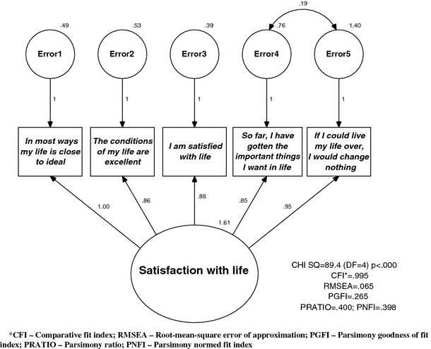
The best fitting model, with unstandardized estimates, based on results of Confirmatory Factor Analysis of the five items in the Satisfaction with Life Scale. This modified one-factor model (correlation between item 4 and 5) was used for all further analyses (Norwegian health interview survey 2005; N = 4,984)
-
4.
A model testing for inter-item correlation when the items were presented consecutively and successively rather than scattered throughout the questionnaire [34]

As the chi² has been shown to be problematic for assessing model fit in large samples [33, 35], model fit was primarily assessed using the root mean square error of approximation (RMSEA) with values of 0.08, 0.05, and 0, and the comparative fit index (CFI), with values 0.90, 0.95, and 1.0 demonstrating reasonable, close, and exact fit, respectively. It is strongly recommended to include measures of parsimony that control for degrees of freedom, especially when testing complex models [33, 35]. Parsimony was evaluated here using the parsimony ratio (PRATIO), the parsimony goodness of fit index (PGFI) and the parsimony normed fit index (PNFI).
Testing of measurement invariance was conducted by multigroup CFAs using ML estimation in AMOS 17. This method employs successive analyses where constraints to the models are added consecutively. The baseline model is an unconstrained model, with one-factor loading constrained to unity. The weak (metric) model, nested under the baseline model, constrains the factor loadings to be equal across groups. Non-significance at this level allows comparing relationships. The strong (scalar) model also constrains factor loadings and intercepts to equality across comparison groups, thus allowing comparing means, and the strict model additionally constrains the residuals. Invariance at the strict level is very seldom achieved.
The chi² alone was not deemed useable in this large sample, but the ΔChi² was measured and reported when comparing the model fit in different subgroups. The ΔCFI was considered a more appropriate test, however, and a cut-off ≤0.01 has been suggested when testing for significant differences between subgroups [33, 35].
Partial measurement invariance was examined with a successive removal of constraints at each level of invariance testing based on examination of modification indices [36]. Level 1 removed constraints on factor loadings one by one. Thereafter constraints were removed for the intercepts keeping the factor loading structure achieved in the partial variance testing at level 1. This method was then repeated at the strict level with progressive removal of constraints on the variances [37]. Tables 5 and 6 indicate which parameters are constrained at each level.
Results
Descriptives
The average response category endorsed by respondents for items 1 through 5 of the SWLS were 5.1, 5.6, 5.6, 5.3, and 4.6, respectively, on a scale of 1–7. Cronbach’s alpha was estimated to be 0.91. This is consistent with values found elsewhere in the literature [16, 38].
Common factoring with principal axis extraction and varimax rotation resulted in 74% of variance explained by a single factor.
Dimensionality
CFAs were then used to compare a one-factor (F1) to a two-factor solution (F2). The two-factor model including “past” (last two items) and “present” (first three items) factors yielded better fit than the unconstrained one-factor model (CFI = 0.995 vs. 0.986); RMSEA = 0.065 vs. 0.094). However, the correlation between the factors was close to unity (r = 0.93), indicating that the two factors could not be easily differentiated. In addition, parsimony was slightly better with the unidimensional model (PNFI: F1 = 0.493, F2 = 0.398).Footnote 1
A modified unidimensional model allowing the residual variance for items 4 and 5 to correlate (F1cov) showed improved fit relative to the baseline model (CFI: F1 = 0.986, F1cov = 0.995; RMSEA: F1 = 0.094, F1cov = 0.065) and identical fit to the two-factor solution (Fig. 1), since the two models are equivalent [39]. This latter model reflects, however, the time dependency in items 4 and 5 more specifically.
A fourth variant suggested by Vautier [34] tested for inter-item correlation when the items were presented to the participants consecutively and successively rather than scattered throughout the questionnaire. The fit of this model was very high (CFI = 0.999; RMSEA = 0.043), but consideration of parsimony indicated that this model should be rejected (PNFI = 0.100, P6FI = 0.067).
Since the correlation between the two factors in the two-factor model was very high (0.93) and minor secondary factors are inherent in most psychological measures [17], the modified single-factor model (Fig. 1) was retained for the subsequent analyses.
Table 3 and Fig. 1 shows the factor loadings and fit measures for the modified single-factor model—for the total sample and for the different subgroups. The factor loadings showed basically the same pattern across subgroups and were generally high (>0.70). For the youngest age group, however, factor loadings for items 4 and 5 were estimated to be <0.70 and relatively lower for item 2 (0.72) than observed in the remaining age groups (0.82–0.90). In the oldest age group, the factor loading for item 5 was also <0.70.
Since the responses are based on a 7-point Likert scale, we assumed continuous variables. The analyses were repeated using Bayesian techniques, however, which are recommended for ordinal data. The results from the two estimation techniques were identical principally to the third decimal (Table 4).
To further examine the effect of the non-normality of the data on results obtained using ML estimation, we also reran the analysis (main model, Fig. 1) using asymptotically distribution free (ADF) testing on the original data set (Table 4). Comparing results from ML estimation with ADF testing resulted in very similar estimates of factor loadings and variance, and all parameters were significant using both methods. Model fit using ADF testing was slightly worse when measured by CFI and PNFI and slightly better when measured by RMSEA.
To further examine the effect of non-normality of the data, the ML testing were repeated on data normalized using Tukey’s formula. The estimated factor loadings, intercepts, and variance differed as expected from those based on ML estimation. The factor loadings remained, however, significant, but the intercepts were no longer found to be significant. Additionally, tests of model fit resulted in worse fit as measured by CFI and parsimony (Table 4).
Finally, bootstrapping, the recommended analysis technique for non-normal data, confirmed the results obtained with standard ML estimation and indicated significance for factor loadings, intercepts, and variance (Table 4).
A total assessment based on Table 4, thus seems to indicate that ML yields satisfactory results even when accounting for the non-normality and ordinal nature of the data.
Measurement invariance
Gender
The results of the tests for multigroup invariance between genders are given in Table 5. No significant differences in Δchi2 were found, indicating weak (metric) invariance between the sexes. Both the strong and the strict invariance tests indicated significant differences across men and women. Due to the large sample sizes, tests involving chi² can be misleading, however. We therefore used the ΔCFI test which is more appropriate for large sample sizes [33, 40]. The ΔCFI results (Table 5) indicate measurement invariance at the weak, strong, and strict levels between genders. Partial invariance techniques indicated invariance at the strict level.
Model fit as measured by RMSEA improved as more constraints were imposed to the model while fit measured by CFI remained consistently high.
Age groups
Results of the tests for multigroup invariance between age groups are shown in Table 6. All three tests (weak, strong, strict) indicated non-invariance across age as measured by significant differences in Δchi². The ΔCFI test, however, indicated invariance at the weak level, but not at the strong or strict levels of invariance testing. Partial invariance testing, however, did indicate invariance at the weak level when removing constraints on factor loadings for item 1 (data not shown), as well as better model fit. Further testing of partial invariance at the strong and strict level did not support measurement invariance across age. In conclusion, the finding of invariance at the weak level assures that comparisons can be made as to the relationships between the factors (factor coefficients) across age groups. The results indicate, however, that caution should be used in analyses involving comparison of means between groups.
Discussion
The Satisfaction with Life Scale [3] is perhaps the most widely used measure of well-being worldwide. The dimensionality of SWLS has been widely discussed, but most studies have been based on specialized sample groups limited in size and biased with respect to gender, age, and relevant socio-demographic parameters. This study aimed to examine the dimensionality of the SWLS in a large and representative sample from Norway (including nearly 5,000 respondents), and to study the robustness of the scale in different subpopulations. This was done by exploring the (1) dimensional structure and (2) measurement invariance across gender and age. No other study has studied dimensionality or subgroup invariance across a continuous age distribution in a comparatively large community sample.
This study also examined the comparability of results from different estimation techniques, including standard ML estimation using raw scores, Bayesian estimation, ADF estimation, and ML estimation using normalized data. The results were consistent regardless of estimation technique, indicating that use of standard ML estimation is satisfactory when studying dimensionality of SWLS when scored on a 7-point Likerts scale.
Dimensions
Our data essentially support a single-factor solution for the SWLS with 74% of variance explained by this single factor. The loadings are on the high side compared to previous studies, and there is a tendency for the last two items to load on a second, less important factor reflecting past accomplishments. This finding is in accordance with several previous reports, but the finding has been interpreted differently across the studies. The correlation between the two factors estimated in this study was very high (r = 0.93), however, and similar to previously reported estimates [14, 18], indicating that the two factors could not be easily differentiated. A post-hoc modification test on the data showed gained fit for the single-factor model when allowing the residual variances for items 4 and 5 to be correlated. This modified single-factor model improved the fit relative to the baseline model and produced fit measures identical to the two-factor model. The single-factor model also agrees with the theoretical development of the scale and measurement processes have been shown to elicit minor secondary factors for psychological measures [17]. In consideration of the arguments put forth by Vautier [34], a separate test of the effect of successive as opposed to scattered positioning of the 5 items of SWLS was therefore performed. This model was rejected based on parsimony. Taken together, our results therefore indicate that a single factor is sufficient to explain the data in this large community sample and even more importantly that the SWLS can be regarded as reflecting a single underlying dimension across the entire adult life span.
The two last items obviously share residual variance over and above what is accounted for by the main latent construct. In the present study, for example, the single-factor model fitted the data better for men than for women, and gave better fit for the two youngest age groups than for the two older age groups. Despite the fact that the last items, perhaps due to their reference to past accomplishments rather than current conditions, appear to involve a somewhat different cognitive search, the overall results support a single dimension in all the subgroups investigated.
Invariance
Between genders
No gender differences were observed at the level of factor loadings, indicating metric or “weak” invariance across gender in the total sample. This attests that the latent variable is related to the items in the same way for men and women. Further constraints equating the intercepts (strong invariance) and the residuals (strict invariance) resulted in significantly reduced fit in terms of the chi² test. Analyses based on large samples may result in high chi² values, however, and increased risk for rejecting good models. In the current study, additional fit indices were either improved (RMSEA) or only slightly decreased (CFI) when adding further constraints (equating intercepts and residuals) to the baseline model. This suggests that the intercepts and residuals may be fixed to equality in men and women, thereby supporting the assumption of strict invariance across gender. This implies that group means on the latent variable as well as analyses involving correlations with the latent variable are comparable across gender. This finding corroborates a number of previously described findings [14, 18, 21, 41], although Atienza et al. [25] in Spanish junior high students did not agree.
Between age groups
People differ in what they require for a satisfying life, and different dimensions of well-being seem to be meaningful to people of varying age. Different ages and life circumstances may cause systematic shifts in how people evaluate their life situation. Oishi and colleagues [42] have, for example, proposed a “value as moderator model” which predicts that as individual’s age, changes in values lead to changes in the determinants of their life satisfaction. Ryff [43] found middle-aged individuals to stress the importance of self-confidence, self-acceptance, job, and career issues, whereas older respondents focus more on health issues. In the present analyses, we find that the SWLS is sensitive to age at the strong and strict levels indicating that life satisfaction as measured by the SWLS does not have the same meaning across the life span.
The results from our current study also indicate that the underlying construct is not fully comparable across the age groups. Our finding is in accordance with previous reports, [14, 26] although others [13, 22–24] found invariance among age groups. These studies were based on far more age homogenous samples (mainly students) and were therefore not able to examine invariance across the entire adult life span. By including respondents from 15 to 79 years, the present study shows that intercepts and residuals vary across the adult life span. Manifest and latent SWLS scores are therefore only partially comparable across age groups. This important finding may partly be due to different adaptation strategies, cohort effects, socialization practises, age specific circumstances influencing interpretations, and conceptualizations of the items on the SWLS as well as increased individual differences in physical health and mobility [44]. Older individuals have been shown to make more global evaluations, be more present oriented and to stress interpersonal aspects, whereas younger people focus more on intrapersonal and specific evaluations [44]. The temporal framing of the items may also be important. The SWLS scale incorporates items referring to both current conditions and past accomplishments, and the time perspectives are likely to vary across age groups [16].
Strengths and limitations of this study
Our study has two major advantages: (1) the relatively large sample size and (2) respondents representing the entire country—all levels of society and a large age span. The shortcomings are related to a moderate response rate, perhaps leading to a less representative sample. When compared to population statistics, women and the age group from 45 to 64 years are overrepresented in this study. The eldest population group (>65 years) consists of fewer individuals, and only includes those living at home, and not in institutions. Likewise, immigrants with a non-Western ethnic background are clearly underrepresented in this material. In addition, using the AMOS analytical package did not allow robust ML testing (Satorra-Bentler scaled statistic) that would have strengthened the analysis when using ordinal non-normal data.
Conclusions
The overall results indicate that the one-factor latent structure of the SWLS is valid in the Norwegian data and that comparing men and women is feasible whereas some caution should be exerted when comparing age groups.
Notes
Detailed results of the analyses of these two models and the model for inter-item correlation is available from the corresponding author.
Abbreviations
- AMOS:
-
Analysis of moment structures
- CFA:
-
Confirmatory factor analysis
- CFI:
-
Comparative fit index
- CI:
-
Confidence interval
- EM:
-
Expectation-Maximization
- ML:
-
Maximum likelihood
- PGFI:
-
Parsimony goodness of fit index
- PRATIO:
-
Parsimony ratio
- PNFI:
-
Parsimony normed fit index
- RMSEA:
-
Root mean square error of approximation
- SE:
-
Standard error
- SPSS:
-
Statistical Package for Social Sciences
- SWLS:
-
Satisfaction with life score
- F1:
-
Simple one-factor model
- F2:
-
Two-factor model
- F1cov:
-
One-factor model with covariance between residuals of items 4 and 5
- ADF:
-
Asymptotically distribution free
References
Cummins, R. A., & Nistico, H. (2002). Maintaining life satisfaction: The role of positive cognitive bias. Journal of Happiness Studies, 3, 37–69.
Diener, E., Emmons, R. A., Larsen, R. J., & Griffin, S. (1985). The satisfaction with life scale. Journal of Personality Assessment, 49, 71–75.
Pavot, W., Diener, E., Colvin, C. R., & Sandvik, E. (1991). Further validation of the satisfaction with life scale: Evidence for the cross-method convergence of well-being measures. Journal of Personality Assessment, 57, 149–161.
Fujita, F., Diener, E., & Sandvik, E. (1991). Gender differences in negative affect and well-being: The case for emotional intensity. Journal of Personality and Social Psychology, 61, 427–434.
Lucas, R. E., & Fujita, F. (2000). Factors influencing the relation between extraversion and pleasant affect. Journal of Personality and Social Psychology, 79, 1039–1056.
Stubbe, J. H., Posthuma, D., Boomsma, D. I., & De Geus, E. J. (2005). Heritability of life satisfaction in adults: A twin-family study. Psychological Medicine, 35(11), 1581–1588.
Lucas, R. E., Diener, E., & Suh, E. (1996). Discriminant validity of well-being measures. Journal of Personality and Social Psychology, 71, 616–628.
Pavot, W., & Diener, E. (1993). Review of the Satisfaction with Life Scale. Psychological Assessment, 5, 164–172.
Anaby, D., Jarus, T., & Zumbo, B. (2010). Psychometric evaluation of the Hebrew language version of the Satisfaction with Life Scale. Social Indicators Research, 96, 267–274.
Arrindell, W. A., Heesink, J., & Feij, J. A. (1999). The Satisfaction with Life Scale (SWLS): Appraisal with 1700 healthy young adults in The Netherlands. Personality and Individual Differences, 26, 815–826.
Balatsky, G., & Diener, E. (1993). A comparison of the well-being of Soviet and American students. Social Indicators Research, 28, 225–243.
Lewis, C. A., Shevlin, M. E., Smekal, V., & Dorahy, M. J. (1999). Factor structure and reliability of a Czech translation of the Satisfaction with Life Scale among Czech university students. Studia Psychologica, 41, 239–244.
Gouveia, V., Milfont, T., da Fonseca, P., & Coelho, J. (2009). Life satisfaction in Brazil: Testing the psychometric properties of the Satisfaction with Life Scale (SWLS) in five Brazilian samples. Social Indicators Research, 90, 267–277.
Hultell, D., & Gustavsson, J. P. (2008). A psychometric evaluation of the Satisfaction with Life Scale in a Swedish nationwide sample of university students. Personality and Individual Differences, 44, 1070–1079.
Oishi, S. (2006). The concept of life satisfaction across cultures: An IRT analysis. Journal of Research in Personality, 40, 411–423.
Pavot, W., & Diener, E. (2008). The Satisfaction with Life Scale and the emerging construct of life satisfaction. The Journal of Positive Psychology: Dedicated to furthering research and promoting good practice, 3, 137–152.
Slocum-Gori, S., Zumbo, B., Michalos, A., & Diener, E. (2009). A note on the dimensionality of quality of life scales: An illustration with the Satisfaction with Life Scale (SWLS). Social Indicators Research, 92, 489–496.
Wu, Ch., & Yao, G. (2006). Analysis of factorial invariance across gender in the Taiwan version of the Satisfaction with Life Scale. Personality and Individual Differences, 40, 1259–1268.
Sachs, J. (2003). Validation of the Satisfaction with Life Scale in a sample of Hong Kong university students. Psychologia: An International Journal of Psychology in the Orient, 46, 225–234.
McDonald, R. P. (1999). Test theory: A unified treatment. Mahwah, N.J: Lawrence Erlbaum Associates.
Shevlin, M., Brunsden, V., & Miles, J. N. V. (1998). Satisfaction With Life Scale: analysis of factorial invariance, mean structures and reliability. Personality and Individual Differences, 25, 911–916.
Blais, M. R., Vallerand, R. J., Pelletier, L. G., & Briere, N. M. (1989). L’echelle de satisfaction de vie: Validation Canadienne-Francaise du “Satisfaction With Life Scate” [French-Canadian validation of the Satisfaction With Life Scale]. Canadian Journal of Behavioral Science, 21, 210–223.
Durak, M., Senol-Durak, E., & Gencoz, T. (2010). Psychometric properties of the Satisfaction with Life Scale among Turkish university students, Correctional officers, and elderly adults. Social Indicators Research. doi:10.1007/s11205-010-9589-4.
Siedlecki, K. L., Tucker-Drob, E. M., Oishi, S., & Salthouse, T. A. (2008). Life satisfaction across adulthood: Different determinants at different ages? The Journal of Positive Psychology, 3, 153–164.
Atienza, F. L., Balaguer, I., & Garcia-Merita, M. L. (2003). Satisfaction with Life Scale: Analysis of factorial invariance across sexes. Personality and Individual Differences, 35, 1255–1260.
Pons, D., Atienza, F. L., Balaguer, I., & Garcia-Merita, M. L. (2000). Satisfaction with Life Scale: Analysis of factorial invariance for adolescents and elderly persons. Perceptual and Motor Skills, 91, 62–68.
Tucker, K., Ozer, D., Lyubomirsky, S., & Boehm, J. (2006). Testing for measurement invariance in the Satisfaction with Life Scale: A comparison of Russians and North Americans. Social Indicators Research, 78, 341–360.
Arbuckle, J. L., & Wothke, W. (2008). AMOS 17.0 User’s Guide. Chicago: SPSSinc.
Rhemtulla, M., Brosseau-Liard, P., & Savalei, V. (2010). How many categories is enough to treat data as continuous? A comparison of robust continuous and categorical SEM estimation methods under a range of non-ideal situations. Manuscript under review, pp. 1–51.
Bollen, K. (1989). Sructural equations with latent variables. New York: John Wiley.
Ory, D. T., & Mokhtarian, P. L. (2010). The impact of non-normality, sample size and estimation technique on goodness-of-fit measures in structural equation modeling: Evidence from ten empirical models of travel behavior. Quality & Quantity, 44, 427–445.
West, S. G., Finch, J. F., & Curran, P. J. (1995). Structural equation models with non-normal variables: Problems and remedies. In R. H. Hoyle (Ed.), Structural equation modeling: Concepts issues and applications (pp. 56–75). Thousand Oaks: Sage.
Byrne, B. M. (2010). Structural equation modeling with AMOS-basic concepts, applications and programming. New York, London: Routledge, Taylor and Francis group, LLC.
Vautier, S., Mullet, E., & Jmel, S. (2004). Assessing the structural robustness of self-rated Satisfaction With Life: A SEM analysis. Social Indicators Research, 68, 235–249.
Hooper, D., Coughlan, J., & Mullen, M. R. (2008). Structural equation modelling: Guidelines for determining model fit. The Electronic Journal of Business Research Methods, 6, 53–60.
Byrne, B. M., Shavelson, R. J., & Muthen, B. (1989). Testing for the equivalence of factor covariance and mean structures: The issue of parital measurement invariance. Psychological Bulletin, 105, 456–466.
Brown, T. A. (2006). Confirmatory factor analysis for applied research. New York: The Guilford Press.
Vassar, M. (2008). A note on the score reliability for the Satisfaction With Life Scale: An RG study. Social Indicators Research, 86, 47–57.
MacCallum, R. C., Wegener, D. T., Uchino, B. N., & Fabrigar, L. R. (1993). The problem of equivalent models in applications of covariance structure analysis. Psychological Bulletin, 114, 185–199.
Meade, A. W., Johnson, E. C., & Braddy, P. W. (2008). Power and sensitivity of alternative fit indices in tests of measurement invariance. Journal of Applied Psychology, 93, 568–592.
Swami, V., & Chamorro-Premuzic, T. (2009). Psychometric evaluation of the Malay Satisfaction With Life Scale. Social Indicators Research, 92, 25–33.
Oishi, S., Diener, E., Suh, E., & Lucas, R. E. (1999). Value as a moderator in subjective well-being. Journal of Personality, 67, 157–184.
Ryff, C. D. (1989). In the eye of the beholder: Views of psychological well-being among middle-aged and older adults. Psychology and Aging, 4, 195–201.
Westerhof, G. J., Dittmann-Kohli, F., & Thissen, T. (2001). Beyond life satisfaction: Lay conceptions of well-being among middle-aged and elderly adults. Social Indicators Research, 56, 179–203.
Acknowledgments
We would like to thank the Norwegian Directorate of Health for financing the study, as well as Statistics Norway for handling the data collection.
Open Access
This article is distributed under the terms of the Creative Commons Attribution Noncommercial License which permits any noncommercial use, distribution, and reproduction in any medium, provided the original author(s) and source are credited.
Author information
Authors and Affiliations
Corresponding author
Rights and permissions
Open Access This is an open access article distributed under the terms of the Creative Commons Attribution Noncommercial License (https://creativecommons.org/licenses/by-nc/2.0), which permits any noncommercial use, distribution, and reproduction in any medium, provided the original author(s) and source are credited.
About this article
Cite this article
Clench-Aas, J., Nes, R.B., Dalgard, O.S. et al. Dimensionality and measurement invariance in the Satisfaction with Life Scale in Norway. Qual Life Res 20, 1307–1317 (2011). https://doi.org/10.1007/s11136-011-9859-x
Accepted:
Published:
Issue Date:
DOI: https://doi.org/10.1007/s11136-011-9859-x