Asymptotics for the stationary distribution in a discrete-time two-dimensional quasi-birth-and-death process

Abstract

We consider a discrete-time two-dimensional process $\{(L_{n}^{(1)},L_{n}^{(2)})\}$ on $\mathbb{Z}_{+}^{2}$ with a background process {J _n } on a finite set, where individual processes $\{L_{n}^{(1)}\}$ and $\{L_{n}^{(2)}\}$ are both skip free. We assume that the joint process $\{Y_{n}\}=\{(L_{n}^{(1)},L_{n}^{(2)},J_{n})\}$ is Markovian and that the transition probabilities of the two-dimensional process $\{(L_{n}^{(1)},L_{n}^{(2)})\}$ are modulated depending on the state of the background process {J _n }. This modulation is space homogeneous, but the transition probabilities in the inside of $\mathbb{Z}_{+}^{2}$ and those around the boundary faces may be different. We call this process a discrete-time two-dimensional quasi-birth-and-death (2D-QBD) process, and obtain the decay rates of the stationary distribution in the coordinate directions. We also distinguish the case where the stationary distribution asymptotically decays in the exact geometric form, in the coordinate directions.

Appendices

Appendix A: Some vectors in Theorem 3.1

Here we give $\tilde{\boldsymbol{g}}^{(1)}_{i}(z_{1}^{\max}),\, i=1,2,3$, by following Li and Zhao [12]; $\tilde{\boldsymbol {g}}^{(2)}_{i}(z_{1}^{\max}), i=1,2,3$, are analogously given and we therefore omit them. Denote by $J(z_{1}^{\max})$ the Jordan canonical form of $R_{1}(z_{1}^{\max })$, then by using a nonsingular matrix $T(z_{1}^{\max})$, it is represented as

where we use $\underline{z}_{2}(z_{1}^{\max})=\bar{z}_{2}(z_{1}^{\max})$ and define $\varLambda(z_{1}^{\max})$ as $\varLambda(z_{1}^{\max})= \operatorname{diag}(J_{k}(z_{1}^{\max}), k\nobreak=2,3,\ldots ,m_{0})$; m ₀ is the number of different eigenvalues of $R(z_{1}^{\max})$ and $J_{k}(z_{1}^{\max}),\ k\nobreak=2,3,\ldots,m_{0}$, are the Jordan blocks. We denote $T(z_{1}^{\max})^{-1}$ in the following block form:

where $t_{11}(z_{1}^{\max})$ is a scalar, $T_{12}(z_{1}^{\max})$ a row vector with dimension s ₁₁−1, $T_{21}(z_{1}^{\max})$ a column vector with the same dimension, and $T_{22}(z_{1}^{\max})$ a square matrix with the same dimension. We also represent $\boldsymbol{w}_{1}^{(1)} N_{1}(z_{1}^{\max}) T(z_{1}^{\max})$ in the following block form:

where ψ is a scalar and ψ a row vector with dimension s ₁₁−1. In terms of the notations above, $\tilde {\boldsymbol{g}}^{(1)}_{i}(z_{1}^{\max}),\, i=1,2,3$, are given as

(36)

(37)

(38)

Appendix B: Proof of Proposition 4.2

Proof

Define diagonal matrix Δ _x as $\varDelta _{\boldsymbol{x}}=\operatorname{diag}\ \boldsymbol{x}$ and matrix Q as $Q= \varDelta _{\boldsymbol{x}}^{-1} (z R^{(1)})^{\top} \varDelta _{\boldsymbol{x}}$. This Q is stochastic since, from the definition, we have Q≥O and $Q \boldsymbol{e}= \varDelta _{\boldsymbol{x}}^{-1} (z \boldsymbol{x}R^{(1)})^{\top}= \varDelta _{\boldsymbol{x}}^{-1} \boldsymbol{x}^{\top}= \boldsymbol{e}$. Furthermore, Q is irreducible since R ⁽¹⁾ is irreducible by Assumption 2.5. From the matrix-geometric form (3), we have, for any n≥1,

We consider two cases for Q; one is that Q is positive recurrent and the other that Q is not positive recurrent.

The case where Q is positive recurrent::

We denote by π=(π _k,j ) the stationary distribution of the stochastic matrix Q. From the assumption $\bar {d}_{1}(z,\boldsymbol{x})<\infty$, we have

$$\sup_{k\ge0} \max_{j\in\mathcal{S}_1(k)} \frac{\nu _{1,k,j}}{x_{k,j}} = \sup_{k,j} \frac{\nu_{1,k,j}}{x_{k,j}} < \infty. $$

Thus, by the bounded convergence theorem and by the limit theorem for Markov chains, we obtain

where $d_{1}^{\dagger}= \sum_{k\ge0} \sum_{j\in\mathcal{S}_{1}(k)} \frac{\nu_{1,k,j}}{x_{k,j}} \pi_{k,j}$.

The case where Q is not positive recurrent::

In this case, Q is null recurrent or transient, and we cannot use the limit theorem for Markov chains to obtain inequalities (26). Hence we apply a technique used in the proof of Proposition 3.2 of Miyazawa [16] to this case. From the assumption $\bar{d}_{1}(z,\boldsymbol{x})<\infty$, there exists an integer k ₀ for any ε>0 such that

$$\max_{j\in\mathcal{S}_1(k)} \frac{\nu_{1,k,j}}{x_{k,j}} \le\bar{d}_1(z, \boldsymbol{x}) + \varepsilon,\quad k>k_0. $$

Thus, we have

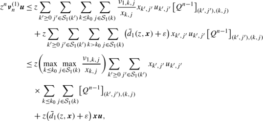
where we use the fact that Q is stochastic. Since Q is null recurrent or transient and ε is arbitrary, we obtain, by the dominated convergence theorem,

$$\limsup_{n\to\infty} z^n \boldsymbol{\nu}_n^{(1)} \boldsymbol{u} \le z \bar{d}_1(z,\boldsymbol{x})\,\boldsymbol{x} \boldsymbol{u}. $$

Thus, setting $\bar{d}_{1}^{\dagger}(\boldsymbol{x})$ as $\bar {d}_{1}^{\dagger}(\boldsymbol{x})=\max(d_{1}^{\dagger},\bar {d}_{1}(z,\boldsymbol{x}))$, we obtain the right hand side inequality of expression (26). The left hand side inequality of expression (26) is analogously obtained, where $\underline{d}_{1}^{\dagger}(\boldsymbol{x})$ is set as $\underline{d}_{1}^{\dagger}(\boldsymbol{x})=\min(d_{1}^{\dagger},\underline{d}_{1}(z,\boldsymbol{x}))$. If Q is positive recurrent, then $d_{1}^{\dagger}>0$. This implies that if $\underline {d}_{1}(z,\boldsymbol{x})>0$, then we always have $\underline {d}_{1}^{\dagger}(\boldsymbol{x})>0$. □

Appendix C: Proof of Proposition 4.4

Proof

Let $\underline{\xi}_{1}^{*}$ and $\underline{\xi}_{2}^{*}$ be defined as

$$\underline{\xi}_1^* = \inf_{k\in\mathbb{Z}_+,\,j\in\mathcal {S}_1(k)} \underline{ \xi}_1(k,j),\qquad\underline{\xi}_2^* = \inf_{k\in\mathbb{Z}_+,\,j\in\mathcal{S}_2(k)} \underline{\xi}_2(k,j). $$

For $\beta_{1}\in[0,\underline{\xi}_{1}^{*}]$ and for $\beta_{2}\in [0,\underline{\xi}_{2}^{*}]$, we define functions f ₁(β ₂) and f ₂(β ₁) as follows:

In the definition of f ₁(β ₂), since we have $\theta_{2} < \beta _{2} \le\underline{\xi}_{2}^{*}$, θ ₁ and θ ₂ satisfy condition (31) of Corollary 4.2 and we obtain $\theta_{1} \le\underline{\xi }_{1}^{*}$. This implies that $f_{1}(\beta_{2}) \le\underline{\xi}_{1}^{*}$. Through the same argument, we also obtain $f_{2}(\beta_{1}) \le\underline {\xi}_{2}^{*}$. We next inductively define the following sequences $\beta_{1}^{(n)}$ and $\beta_{2}^{(n)}$ for n∈ℤ₊ with $\beta_{1}^{(0)}=\beta _{2}^{(0)}=0$:

Since $\beta_{2}^{(0)}=0\le\underline{\xi}_{2}^{*}$, we inductively obtain $\beta_{1}^{(n)}\le\underline{\xi}_{1}^{*}$ and $\beta_{2}^{(n)}\le \underline{\xi}_{2}^{*}$ for all n=0,1,… By the definitions, f ₁(x) and f ₂(x) are obviously nondecreasing in x, and hence f ₁(f ₂(x)) and f ₂(f ₁(x)) are also nondecreasing in x. For i=1,2, since and $\beta_{i}^{(0)}=0\le\beta_{i}^{(1)}$, we inductively obtain, for any n≥1,

$$\beta_i^{(n+1)}-\beta_i^{(n)} = f_i \bigl(f_{3-i} \bigl(\beta_i^{(n)} \bigr)-f_i \bigl(f_{3-i} \bigl(\beta_i^{(n-1)} \bigr) \bigr)\ge0. $$

Thus, $\beta_{1}^{(n)}$ and $\beta_{2}^{(n)}$ are bounded and nondecreasing in n, and this implies that the limits of them exist; we denote the limits by $\beta_{1}^{(\infty)}$ and $\beta_{2}^{(\infty )}$, respectively. Then, we have

Thus, for i=1,2, if we can prove that $\beta_{i}^{(\infty)} = \zeta _{i}$, then we obtain $\zeta_{i}\le\underline{\xi}_{i}^{*}$.

To this end, we first prove that $\beta_{1}^{(n)}\le\zeta_{1}$ and $\beta_{2}^{(n)}\le\zeta_{2}$ for all n∈ℤ₊. By the definitions of and , f ₁(β ₂) and f ₂(β ₁) are represented as

This implies that $\beta_{1}^{(n)}\le\theta_{1}^{(c)}$ and $\beta _{2}^{(n)}\le\eta_{2}^{(c)}$ for all n∈ℤ₊. Since $\log\underline{z}_{2}(e^{s})$ is convex in $s\in[0,\theta _{1}^{\max}]$, if $\beta_{2}\le\theta_{2}^{\max}$ then “$\log \underline{z}_{2}(e^{\theta_{1}})< \beta_{2}$” implies that $\theta_{1} < \log\bar{z}_{1}(\beta_{2})$, otherwise it implies that $\theta_{1} < \theta_{1}^{\max}$. Thus we obtain

Note that $\log\bar{z}_{1}(e^{s})$ is concave and increasing in $s\in [0,\theta_{2}^{\max}]$. For a given n, consider $f_{1}(\beta_{2}^{(n)})$ in three cases, as follows. (a) If $\beta_{2}^{(n)}\le\theta_{2}^{(c)}\le\theta_{2}^{\max}$, then we have $\log\bar{z}_{1}(e^{\beta_{2}^{(n)}})\le\log\bar {z}_{1}(e^{\theta_{2}^{(c)}})=\theta_{1}^{(c)}$. Thus, if (C1) or (C3) holds, we have $\zeta_{1}=\theta_{1}^{(c)}$; if (C2) holds, we have $\beta_{2}^{(n)}\le\eta_{2}^{(c)}\le\theta_{2}^{(c)}$ and $\log\bar {z}_{1}(e^{\beta_{2}^{(n)}})\le\log\bar{z}_{1}(e^{\eta_{2}^{(c)}})=\bar {\eta}_{1}^{(c)}=\nobreak\zeta_{1}$. We, therefore, obtain $\min\{\log\bar {z}_{1}(\beta_{2}),\,\theta_{1}^{(c)}\}=\log\bar{z}_{1}(\beta_{2}^{(n)})\le \zeta_{1}$. (b) If $\theta_{2}^{(c)}< \beta_{2}^{(n)}\le\theta_{2}^{\max}$, then we have $\theta_{1}^{(c)}=\log\bar{z}_{1}(e^{\theta_{2}^{(c)}})<\log\bar {z}_{1}(e^{\beta_{2}^{(n)}})$. Furthermore, we have $\theta_{2}^{(c)}< \beta_{2}^{(n)}\le\eta_{2}^{(c)}$ and this implies that (C1) or (C3) holds. Thus, we obtain $\min\{\log\bar{z}_{1}(\beta_{2}^{(n)}),\,\theta _{1}^{(c)}\}=\theta_{1}^{(c)}=\zeta_{1}$. (c) If $\beta_{2}^{(n)}> \theta_{2}^{\max}$, then we have $\theta _{2}^{(c)}\le\theta_{2}^{\max}< \beta_{2}^{(n)}\le\eta_{2}^{(c)}$. This implies that (C1) or (C3) holds and we obtain $\zeta_{1}=\theta_{1}^{(c)}$. As a result, $f_{1}(\beta_{2}^{(n)})$ is given by

Since $f_{1}(\beta_{2}^{(n)})$ and $f_{2}(\beta_{1}^{(n)})$ are symmetric in a certain sense, we also obtain

Next, for a given n, consider $f_{1}(f_{2}(\beta_{1}^{(n)}))$ in four cases, as follows. (a) If $\beta_{1}^{(n)}\le\eta_{1}^{(c)}$ and $\log\bar{z}_{2}(e^{\beta _{1}^{(n)}})\le\theta_{2}^{(c)}$, then we have $f_{1}(f_{2}(\beta _{1}^{(n)}))=\log\bar{z}_{1}(\bar{z}_{2}(e^{\beta_{1}^{(n)}})$. From the fact that $\bar{z}_{2}(\underline{z}_{1}(\bar{z}_{2}(e^{\beta_{1}^{(n)}}))) = \bar{z}_{2}(\bar{z}_{1}(\bar{z}_{2}(e^{\beta_{1}^{(n)}}))) = \bar {z}_{2}(e^{\beta_{1}^{(n)}})$, we have $\beta_{1}^{(n)}$ is given by $\log \underline{z}_{1}(\bar{z}_{2}(e^{\beta_{1}^{(n)}}))$ or by $\log\bar {z}_{1}(\bar{z}_{2}(e^{\beta_{1}^{(n)}}))$, but since $\beta_{1}^{(n)}\le \eta_{1}^{(c)}$, $\beta_{1}^{(n)}$ must be equal to $\log\underline {z}_{1}(\bar{z}_{2}(e^{\beta_{1}^{(n)}}))$, i.e.,

In this expression, equality holds only when $\beta_{1}^{(n)}=\eta _{1}^{(c)}$, and in such a case, since , (C2) holds and we obtain $f_{1}(f_{2}(\beta_{1}^{(n)}))\!=\!\log\bar{z}_{1}(\bar{z}_{2}(e^{\eta _{1}^{(c)}}))\!=\bar{\eta}_{1}^{(c)}=\zeta_{1}$. (b) If $\beta_{1}^{(n)}\le\eta_{1}^{(c)}$ and $\log\bar{z}_{2}(e^{\beta _{1}^{(n)}})> \theta_{2}^{(c)}$, then we have $f_{1}(f_{2}(\beta _{1}^{(n)}))=\theta_{1}^{(c)}$. In this case, (C1) or (C3) is holds and we have $\zeta_{1}=\theta_{1}^{(c)}$. (c) If $\beta_{1}^{(n)}> \eta_{1}^{(c)}$ and $\eta_{2}^{(c)}\le\theta _{2}^{(c)}$, then we have $\eta_{1}^{(c)}<\beta_{1}^{(n)}\le\theta _{1}^{(c)}$. Thus, (C2) holds and we obtain $f_{1}(f_{2}(\beta _{1}^{(n)}))=\log\bar{z}_{1}(e^{\eta_{2}^{(c)}})=\bar{\eta }_{1}^{(c)}=\zeta_{1}$. (d) If $\beta_{1}^{(n)}> \eta_{1}^{(c)}$ and $\eta_{2}^{(c)}> \theta _{2}^{(c)}$, then (C1) holds and we obtain $f_{1}(f_{2}(\beta _{1}^{(n)}))=\theta_{1}^{(c)}=\zeta_{1}$. As a result, $f_{1}(f_{2}(\beta_{1}^{(n)}))$ is given by

(39)

If $\beta_{1}^{(\infty)}<\zeta_{1}$, then by expression (39), we obtain

$$\beta_1^{(\infty)} = f_1 \bigl(f_2 \bigl( \beta_1^{(\infty)} \bigr) \bigr) = \log \bar{z}_1 \bigl( \bar{z}_2 \bigl(e^{\beta_1^{(\infty)}} \bigr) \bigr) > \log\underline{z}_1 \bigl(\bar{z}_2 \bigl(e^{\beta_1^{(\infty)}} \bigr) \bigr) = \beta_1^{(\infty)}, $$

but this is a contradiction. Hence we obtain $\beta_{1}^{(\infty )}=\zeta_{1}$. Through the same argument, we also obtain $\beta _{2}^{(\infty)}=\zeta_{2}$, and this completes the proof. □

References

Boxma, O.J., Groenendijk, W.P.: Two queues with alternating service and switching times. In: Boxma, O.J., Syski, S. (eds.) Queueing Theory and Its Applications, pp. 261–282. North-Holland, Amsterdam (1988)
Fayolle, G., Malyshev, V.A., Menshikov, M.V.: Topics in the Constructive Theory of Countable Markov Chains. Cambridge University Press, Cambridge (1995)
Haque, L., Zhao, Y.Q.: Sufficient conditions for a geometric tail in a QBD process with many countable levels and phases. Stoch. Models 21(1), 77–99 (2005)
He, Q.-M., Li, H., Zhao, T.Q.: Light-tailed behavior in QBD processes with countably many phases. Stoch. Models 25, 50–75 (2009)
Katou, K., Makimoto, N., Takahashi, Y.: Upper bound for the decay rate of the marginal queue-length distribution in a two-node Markovian queueing system. J. Oper. Res. Soc. Jpn. 47, 314–338 (2004)
Katou, K., Makimoto, N., Takahashi, Y.: Upper bound for the decay rate of the joint queue-length distribution in a two-node Markovian queueing system. Queueing Syst. 58, 161–189 (2008)
Kijima, M.: Quasi-stationary distributions of single-server phase-type queues. Math. Oper. Res. 18(2), 423–437 (1993)
Kingman, J.F.C.: A convexity property of positive matrices. Q. J. Math. 12, 283–284 (1961)
Kobayashi, M., Miyazawa, M.: Revisit to the tail asymptotics of the double QBD process: Refinement and complete solutions for the coordinate and diagonal directions. In: Matrix-Analytic Methods in Stochastic Models. Springer, Berlin (2012, to appear)
Latouche, G., Ramaswami, V.: Introduction to Matrix Analytic Methods in Stochastic Modeling. SIAM, Philadelphia (1999)
Li, Q.-L., Zhao, Y.Q.: A constructive method for finding β-invariant measures for transition matrices of M/G/1 type. In: Latouche, G., Taylor, P. (eds.) Matrix-Analytic Methods: Theory and Applications, pp. 237–263. World Scientific, Singapore (2002)
Li, Q.-L., Zhao, Y.Q.: β-invariant measures for transition matrices of GI/M/1 type. Stoch. Models 19(2), 201–233 (2003)
Li, H., Miyazawa, M., Zhao, Y.Q.: Geometric decay in a QBD process with countable background states with applications to a join-the-shortest-queue model. Stoch. Models 23(3), 413–438 (2007)
Li, H., Zhao, Y.Q.: Exact tail asymptotics in a priority queue—characterizations of the non-preemptive model. Queueing Syst. 68(2), 165–192 (2011)
Miyazawa, M., Zhao, Y.Q.: The stationary tail asymptotics in the GI/G/1 type queue with countably many background states. Adv. Appl. Probab. 36(4), 1231–1251 (2004)
Miyazawa, M.: Tail decay rates in double QBD processes and related reflected random walks. Math. Oper. Res. 34(3), 547–575 (2009)
Miyazawa, M.: Light tail asymptotics in multidimensional reflecting processes for queueing networks. Top 19(2), 233–299 (2011)
Motyer, A.J., Taylor, P.G.: Decay rates for quasi-birth-and-death processes with countably many phases and tridiagonal block generators. Adv. Appl. Probab. 38, 522–544 (2006)
Neuts, M.F.: Matrix-Geometric Solutions in Stochastic Models. Dover Publications, New York (1994)
Ozawa, T.: Waiting time distribution in a two-queue model with mixed exhaustive and gated-type K-limited services. In: Hasegawa, T., Takagi, H., Takahashi, Y. (eds.) Performance and Management of Complex Communication Networks, pp. 233–252. Chapman & Hall, London (1998)
Resing, J.A.C.: Polling systems and multiple branching processes. Queueing Syst. 13, 409–426 (1993)
Seneta, E.: Non-negative Matrices and Markov Chains, Revised Printing. Springer, New York (2006)
Takagi, H.: Queueing analysis of polling models: progress in 1990–1994. In: Dshalalow, J.H. (ed.) Frontiers in Queueing: Models, Methods and Problems, pp. 119–146. CRC Press, Boca Raton (1997)
Takagi, H.: Analysis and application of polling models. In: Haring, G., Lindemann, C., Reiser, M. (eds.) Performance Evaluation: Origins and Directions. Lecture Notes in Computer Science, pp. 424–442. Springer, Berlin (2000)
Takahashi, Y., Fujimoto, K., Makimoto, N.: Geometric decay of the steady-state probabilities in a quasi-birth-and-death process with a countable number of phases. Stoch. Models 17(1), 1–24 (2001)
Tweedie, R.L.: Operator-geometric stationary distributions for Markov chains with applications to queueing models. Adv. Appl. Probab. 14, 368–391 (1982)
Winands, E.M.M., Adan, I.J.B.F., van Houtum, G.J., Down, D.G.: A state-dependent polling model with k-limited service. Probab. Eng. Inf. Sci. 23, 385–408 (2009)
Xue, J., Alfa, A.S.: Geometric tail of queue length of low-priority customers in a nonpreemptive priority MAP/PH/1 queue. Queueing Syst. 69(1), 45–76 (2011)
Acknowledgement
The author would like to thank the anonymous reviewers for their valuable comments.
Author information
Authors and Affiliations
Corresponding author