
Abstract
The phenomenon of quasi-periodicity in deterministic dynamical systems describes stationary solutions, which neither exhibit a finite period length nor are chaotic. Recently, an increasing demand for robust numerical methods is driven by applied dynamics and industrial applications. In this context, direct time integration proves to be impractical due to extensive integration intervals. Therefore, in a first step, this contribution aims on giving an application oriented survey of the basic theory as well as alternative concepts. In the following, the focus is set on the direct computation of invariant manifolds (surfaces) on which quasi-periodic solutions evolve. This approach offers a unique framework from which classical methods (e.g., the multi-harmonic-balance) can be systematically deduced and mutual similarities between different methods may be revealed. This contribution starts with a brief summary of related mathematical basics, which is followed by an overview of available methods. Subsequently, the computation of invariant manifolds by means of solving a partial differential equation is emphasized. These PDEs may be formulated using different parametrization strategies. Here, the concept of hyper-time parametrization is particularly interesting, since it is a promising starting point for the development of numerical schemes with general applicability in engineering problems. In order to solve the underlying PDE, various methods may be used. The implementation of a Fourier-Galerkin method as well as a finite difference method is presented and compared on the basis of computational results of the van-der-Pol equation (with and without forcing). Moreover, it is demonstrated that both methods apply to periodic as well as quasi-periodic solutions alike. In order to exemplify the practical use, these methods are applied to a generic rotordynamic model problem.
1 Motivation and introduction
Stationary solutions play a major role in the analysis and characterization of dynamical systems. Within this work, the term “stationary” refers to solution types which persist in infinite time intervals (also called“steady state”). Very well known types of stationary solutions in deterministic systems are equilibria and periodic solutions: such solutions are widely discussed in basic textbooks, well understood and various standard approaches for their efficient analysis are available.
Beyond this, another well-known type of solutions are quasi-periodic motions. While being known at least since the works of Poincaré in the \( 19^{\text {th}}\) century, systematic research with the aim of finding general approaches is a comparatively young field of research (cf. Sect. 1.2). Although it might appear as a mathematical curiosity, quasi-periodicity is frequently encountered in technical applications. Moreover, it is strongly related to the aforementioned types of stationary solutions and could even be seen as a kind of “higher-order” periodicity in the sense of the next logical step after periodic solutions:
-
Equilibrium solutions are non-periodic and thus have no frequency (cf. Fig. 1a)).
-
Periodic solutions are associated with a single frequency, which represents the base frequency of the corresponding Fourier-series. The spectrum is discrete and exhibits frequencies at integer multiples of this single base frequency (cf. Fig. 1b)).
-
Quasi-periodic solutions are characterized by a discrete frequency spectrum, which does not consists of integer multiples of one single base frequency. The spectrum consists of linear combinations of at least two independent base frequencies (cf. Fig. 1c)).
Obviously, all these types of dynamics fit into a common systematization scheme. Here, the notion of frequencies being “independent” is strongly related to incommensurability, which will be explained below.

Relation between different types of stationary solutions based on the number of independent frequencies \(\nu \): (a) equilibrium point, (b) periodic motion, (c) quasi-periodic motion with two independent frequencies
The appearance of multiple independent frequencies can be related to multiple individual sources of vibration, which affect the system simultaneously: for instance, such sources may be co-existing mechanisms of self-excitation or forcing. Due to the presence of multiple independent frequencies, the time signals of quasi-periodic motions do not exhibit a finite period length: therefore standard numerical and analytical approaches for periodic solutions are in general hardly applicable.
Although the theoretical fundamentals of quasi-periodic motions are well studied (cf. [6]), the analysis of such motions in practical applications is scarce. Recent publications started applying selected techniques to identify quasi-periodic motions of flutter vibrations of tuned bladed disks damped by friction [30], quasi-periodic localized vibrations in a bladed disk assembly [19], quasi-periodic motions of rubbing self-induced vibrations in rotor-stator dynamics [40] and quasi-periodic motions of a simplified finite-element model with oil-film forces of a symmetric rotor of a turbocharger [48].
It may be concluded that quasi-periodic motions—being a generalization of periodic ones—are of high relevance in applied dynamics. Unfortunately, only very few publications of the application oriented engineering literature are concerned with corresponding methods and analyses. Therefore, this contribution aims on giving practitioners an access to this topic by giving a brief overview and presenting two different standard methods within a unified framework.
First, common approaches to the topic are discussed and classified. Furthermore, among the available methods two particular methods for the calculation of quasi-periodic motions—namely, a Finite Difference Method and a Fourier-Galerkin method—are presented and discussed in detail. Main reasons for this choice are that these two methods are very popular in engineering dynamics, work independent of the stability of the quasi-periodic motion, can easily be implemented using standard methods, and thus exhibit the potential to be applied to large systems (e.g., FEM models). Moreover, it shall be emphasized that both methods may be derived within a common framework and thus exhibit a high degree of similarity regarding their basic formulation.
1.1 Mathematical definitions
In the following part, some elementary definitions of relevant mathematical terms are given.
-
Incommensurability and frequency basis: [42, p. 9] Let \( \varvec{a} = [\dots , a_k, \dots ]^\top \) be a vector of integer numbers and \( \varvec{\nu } = [\dots , \nu _k, \dots ]^\top \) be a vector of real-valued frequencies. The frequencies \(\nu _k\) are said to be incommensurable (rationally independent), if
$$\begin{aligned} \varvec{a} ^\top \varvec{\nu } = \sum \limits _{k = 1}^p a_k \nu _k = 0 \quad \quad \begin{array}{rl} \varvec{\nu } &{}\in \mathbb {R}^p\\ \varvec{a} &{}\in \mathbb {Z}^p \end{array} \end{aligned}$$(1)only holds for \( \varvec{a} = \varvec{0} \). In other words: for a set of incommensurable frequencies no frequency is an integer multiple or linear-combination of the others. A \( \varvec{\nu } \) for which this condition holds is called a frequency basis. To put this in context, see the following examples:
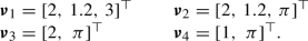
\( \varvec{\nu } _1 \) is not incommensurable, since \( \varvec{a} = [-3,\,10,\,-2]^\top \) fulfills condition (1). \( \varvec{\nu _2 } \) is also not incommensurable since \( \varvec{a} = [-6,\,10,\,0]^\top \) fulfills condition (1). \( \varvec{\nu } _3\) and \( \varvec{\nu } _4 \) are both possible frequency base vectors.
-
Quasi-periodic function: [42, p. 9] If a state \( \varvec{z} (t) \) can be stated as:
$$\begin{aligned} \begin{gathered} \varvec{z} (t) = \varvec{Z} ( \varvec{\nu } t) = \varvec{Z} (\nu _1 t, \dots , \nu _p t) \\ \begin{array}{rl} \varvec{z} &{}: \mathbb {R}^1 \mapsto \mathbb {R}^n, \\ \varvec{Z} &{}: \mathbb {R}^1 \mapsto \mathbb {R}^n, \, \varvec{\nu } \in \mathbb {R}^p \end{array} \end{gathered} \end{aligned}$$(2)with \( \varvec{\nu } \) being a frequency basis, \( p>1 \) and \( { \varvec{Z} } \) being \(2\pi \)-periodic with respect to any argument
$$\begin{aligned} { \varvec{Z} }(...,\nu _k t,...) = { \varvec{Z} }(...,\nu _k t + 2 \pi ,...) ~ \forall k\in [1,\dots ,p] , \end{aligned}$$then \( { \varvec{Z} } \) is called a quasi-periodic function. The function maps from \(t\in \mathbb {R}\) to the n-dimensional state-space. Due to the incommensurability of the \(p>1\) frequencies \( \varvec{\nu } \), the function \( { \varvec{Z} }({ \varvec{\nu } }t) \) does not have a finite period length. For \(p=1\), \({ \varvec{Z} }\) is a periodic function (closed curve in state-space), for \(p=0\), \({ \varvec{Z} }\) represents a constant function (stationary point in state-space).
-
Coordinate torus, torus function and p-torus:
The set of \(2\pi \)-periodic coordinates \( \varvec{\theta } {=} [\theta _1,{...},\theta _p] \in \mathbb {R}^p\mod 2 \pi \) is referred to as coordinate torus and is denoted by \( \mathbb {T}^p \). Here, \( \varvec{\theta } \) is the vector of torus coordinates. The function
$$\begin{aligned} \varvec{Z} ( \varvec{\theta } ) = \varvec{Z} (\theta _1,\dots ,\theta _p) \qquad \varvec{Z} : \mathbb {T}^p \mapsto \mathbb {R}^n, \end{aligned}$$(3)that maps from a p-dimensional coordinate torus to the n-dimensional state-space, is a torus function. The image of \( \varvec{\theta } \) under the function \( \varvec{Z} \) is called p-torus and is a hypersurface with no boundaries embedded in the n-dimensional state-space. In other words, each of the arguments \( \theta _k \) of a torus function \( \varvec{Z} ( \varvec{\theta } ) \) can be chosen independently from each other, whereas the arguments \( \nu _i t \) of a quasi-periodic function \( \varvec{Z} ( \varvec{\nu } t) \) all depend on time t.
-
Density and maxima: [42, p. 10]
The set of values of a quasi-periodic function \( { \varvec{Z} }( \varvec{\nu } t) \), which is an infinitely long trajectory in the state-space is dense in the values \( \varvec{Z} ( \varvec{\theta } ) \). Dense means that for every small \( \varepsilon \) and any \( \varvec{\theta } \) at least one \( \hat{t} \) exists, so that
$$\begin{aligned} \left\Vert \varvec{Z} ( \varvec{\theta } ) - { \varvec{Z} }( \varvec{\nu } \hat{t})\right\Vert < \varepsilon , \quad \quad \varepsilon \ll 1 \end{aligned}$$(4)holds. Thus, the 1-dimensional trajectory \( { \varvec{Z} }( \varvec{\nu } t) \) lies on the p-dimensional surface of the torus \( \varvec{Z} ( \varvec{\theta } ) \) and passes any point of the torus-surface or arbitrarily close to it. Roughly speaking, the curve \( { \varvec{Z} }( \varvec{\nu } t) \), \(t\in \mathbb {R}\) fills the surface \( \varvec{Z} ( \varvec{\theta } )\), \( \varvec{\theta } \in \mathbb {T}^p\) completely (see Fig. 2). In return, everything about the extents of \( { \varvec{Z} }( \varvec{\nu } t)\) will be known as soon as the surface \( \varvec{Z} ( \varvec{\theta } )\) has been determined. It follows that
$$\begin{aligned} \underset{t \in \mathbb {R}^1}{\text {sup}} \left| \varvec{z} (t)\right|= \underset{ \varvec{\theta } \in \mathbb {T}^p}{\text {max}}\left| \varvec{Z} ( \varvec{\theta } )\right|= \left\Vert \varvec{Z} ( \varvec{\theta } )\right\Vert _0 \end{aligned}$$(5)[42, p. 11], which gives the equivalence of the supremum of a quasi-periodic function and the maximum of a torus function.


A torus \( \varvec{Z} ( \varvec{\theta } )\) in state-space about to be filled completely by a quasi-periodic trajectory \( \varvec{z} (t) {= \varvec{Z} ( \varvec{\nu } t)}\)
1.2 Review and classification of numerical approaches
The phenomenon of quasi-periodicity has been known at least since the \( 19{\text {th}} \) century, when Poincaré amongst others worked on integrable Hamiltonian systems. The systematic investigation of quasi-periodic functions started in 1925 within the works of Bohr on almost periodic/quasi-periodic functions [4]. The theory was further developed by Besicovitch [2], von Neumann [38], Bochner [3] and many more. An outline of the historic development can be found in [31].
Since the late 1970s, research started on numerical algorithms, which approximate the invariant p-tori on which the quasi-periodic solutions evolve. The methods can roughly be divided in two groups, which either investigate an invariant closed curve in a Poincaré-section or the invariant manifold (torus). Most of these methods can (sometimes after brief adaption) be used for stable and unstable tori.
The following classification is a slight extension to that given by Schilder et. al [46]. However, the differences between the methods are fluid. More extensive reviews of the methods can be found in [1, 25, 46]. The reader should be aware that apart from the methods detailed below further ones exist in the more theoretical focused literature. However, their application to large engineering systems may be limited. Examples are the algorithms presented in [9, 10], which are based on the parametrization method and identify invariant tori and their invariant normal bundles, as well as the graph transform method, which can be seen as an integral form of the method discussed in Sect. 1.2.2, see [5, 7, 16, 25, 26, 29].
1.2.1 POINCARÉ mapping methods—invariant closed curve approximation
This class of methods is based on identifying an invariant object in an appropriate Poincaré-section in the state-space to circumvent the problems related to the open interval (not finite period length) of the time signal. The invariant object is constructed by using sections of the quasi-periodic trajectory \( \varvec{z} (t)\).
This method is best explained by means of a 2-torus, because the invariant object is in this context a closed curve (1-torus). Assume that a stationary trajectory \( \varvec{z} \) is calculated (e.g., by direct time integration), which fills the p-dimensional torus \( \varvec{Z} (\varvec{\theta }) \subset \mathbb {R}^n,\varvec{\theta }\in \mathbb {T}^2 \) densely. Intersecting this torus with an appropriately defined \((n-1)\)-dimensional hyperplane \(\varSigma \) in the state-space will yield a continuous closed curve (see Fig. 3).

An intersection with a two-dimensional plane \(\varSigma \) leads to an invariant curve, which is densely filled by the intersected quasi-periodic trajectory
Due to the density of \( \varvec{z} \) on the torus, this curve is also densely filled by intersections of \( \varvec{z} \) and \(\varSigma \). Now consider trajectories, which start on some point of this intersection curve: evolving on the torus, they will again reach the curve after a finite time. Thus, using a Poincaré-mapping that maps a starting point on \(\varSigma \) to the corresponding end-point on \(\varSigma \) of a trajectory allows to formulate a shooting-algorithm or collocation-algorithm, that approximates the intersection curve by a finite number of m points. Moreover, once this single intersection curve has been approximated, m-stationary trajectories on the torus are known and thus usually enough data are available to describe the entire torus.
In principle, two conceptional different approaches are used in the literature to approximate the invariant closed curve. The first methodology is based on one trajectory, by which the invariant closed curve in the Poincaré-section is approximated. The trajectory is usually obtained by time integration. This approach was introduced for quasi-periodic solutions by Kaas-Petersen in 1986 [27, 28] and further developed by Ling in 1991 [33]. A more recent application for large systems can be found in [43, 44].
The second methodology is based on multiple trajectories, which approximate the invariant closed curve in the Poincaré-section. Here, all trajectories start and end on the invariant closed curve. As a result, a boundary value problem with periodic boundaries can be deduced. Introduced by Gómez and Mondelo in 2001 [22], the authors used a shooting-method to obtain the trajectories and a Fourier-series to approximate the invariant closed curve. Because the authors focused on the restricted three-body problem, the method is often used in the context of astrodynamics [34, 39]. A review can be found in [1]. Furthermore, the authors of [47] proposed in 2007 a similar approach and gave the interesting note that the continuation program AUTO [14] can be used to solve the boundary value problem with periodic boundaries. Instead of using a shooting-algorithm, Dankowicz and Schilder utilized in [11] a collocation method to discretize the trajectories involved in the boundary value problem. A slight variation to this concept is the flow box tiling method introduced by Henderson [25]: trajectories on the torus are enclosed by boxes, which are variable in size. By imposing boundary conditions on each inset and outset of these boxes, the whole torus can be completely covered with a finite number of boxes, instead of an infinitely long trajectory.
Approaching tori by means of invariant closed circles is geometrically descriptive and identifying one trajectory (first methodology) is a straightforward implementation, by which almost any time integration scheme can be combined with shooting-algorithms. However, despite its appealing simplicity the methods suffer from several drawbacks, as, for instance:
-
Depending on the geometrical complexity of the intersection curve (i.e., the number of points necessary to approximate it) or on the specific base frequencies (i.e., close to synchronized states), it still may demand for a potentially high number of trajectories.
-
The stability of the quasi-periodic motions is a crucial characteristic, because in general the involved time integration diverges if motions are unstable.
The approach by means of multiple trajectories (second methodology) does not depend significantly on the first stated drawback, but in case of an involved shooting-algorithm, the second stated drawback applies as well. This may be circumvented by using multiple shooting-algorithms, by which the calculation effort increases considerably for many trajectories or/and many degrees of freedom. Concerning the collocation method, both of the stated drawbacks do not apply and the interested reader is referred to [11].
1.2.2 Generalized invariance equation methods—torus approximation
This class features several of the most popular methods in the application oriented literature. It is directly based on the ODEs that describe the dynamical system in the state-space:

where it is assumed that \( \varvec{z} \) is a quasi-periodic solution. If the right-hand side does explicitly depend on t, it is required that
holds. Here, m is the number of incommensurable frequencies of the external excitation. Starting from these ODEs, PDEs describing a p-torus are derived. There are two major subclasses, which look very similar, but significantly differ in the basic idea of the parametrization approach:
State-Space Parametrization: The first and crucial step in this approach is to find a local parametrization for the p-torus in state-space and transform the system equations (6) to these new coordinates. A commonchoice are p torus coordinates \( \varvec{\theta } \, \in \mathbb {T}^p\) and \(q=n-p\) local coordinates \( \varvec{u} \in \mathbb {R}^q \), which may often be interpreted as dependent phase angles and amplitudes (cf. [36]).
More formally, the p torus coordinates \( \varvec{\theta } \) describe the local tangential space, while the coordinates \( \varvec{u} \) belong to the q-dimensional normal space of the torus.
Thus, by virtue of \( \varvec{z} (t) = \hat{ \varvec{z} }( \varvec{\theta } {(t)}, \varvec{u} {(t)} ) \), Eq. (6) may be rewritten as a partitioned system
Note that an explicit time dependency in Eq. (6) is considered in Eqs. (8) and (9) in the torus coordinates. Eliminating the time dependency in Eq. (8) and (9)) yields a system of PDEs that expresses \( \varvec{u} = \varvec{u} ( \varvec{\theta } )\) as:
This equation expresses the invariance principle: it describes that any point \( ( \varvec{\theta } , \varvec{u} ) \) on the p-torus is mapped by \( \varvec{R} \) into the tangential subspace of thep-torus spanned by the subspace vectors \( \frac{\partial \varvec{u} ( \varvec{\theta } )}{\partial \theta _j} \). Thus, \( \psi _j \) are the coordinates of the point.
Once \( \varvec{u} = \varvec{u} ( \varvec{\theta } )\) is known, it may be inserted into Eq. (8) yielding
The solution of this equation describes the motion on the torus itself. Since the right-hand side of Eq. (11) is usually not a constant, the tangents of the flow-lines \( \varvec{\theta } (t)\) in general will not have the same direction: thus, the flow on the torus is usually not a parallel flow. By investigating Eq. (11), synchronization of solutions may be detected and analyzed.
This approach offers a rather intuitive way to describe tori and quasi-periodic motions. Consequently, it is often used in analytical investigations of periodic and quasi-periodic motions by transforming to “amplitude” and “phase”-coordinates (or “action” and “angle” for Hamiltonian systems). Moreover, several numerical schemes like Fourier-Galerkin (Samoilenko (1987) [42] and Ge and Leung in 1998 [20]), finite differences (Dieci et. al in 1991 [13]), collocation (Edoh and Russel in 2000 [15]) and many more were used to solve Eq. (10).
However, defining an appropriate torus parametrization for arbitrary problems is very challenging and will demand for a high amount of a priori knowledge about the solution and in particular the geometric features of the torus. Thus, it will only hardly allow for generalized algorithmic implementations. Moreover, carrying out the corresponding nonlinear coordinate transformation usually turns out to be a costly step. Consequently, this approach is usually not applicable to larger problems as they are typical for modern applied dynamics and engineering.
Hyper-Time Parametrization: In contrast to the state-space parametrization, this technique does not require any a priori parametrization or costly transformation steps and thus is suitable to develop algorithms of broad applicability. For this reason, the present publication will focus on this class of methods.
As stated in Sect. 1.1, a general quasi-periodic time function exhibiting a frequency basis of p incommensurable frequencies \(\nu _k\) (\(k=1,\dots ,p\)) may be written as:
where the arguments \(\nu _k t\) depend on t as a single independent variable. This function \({ \varvec{Z} }\) is \(2\pi \)-periodic with respect to any of its p arguments \(\nu _k t\). Thus, to account for these periodicities, p new variables \(\theta _k = \nu _k t \mod 2\pi \in \left[ 0, \, 2\pi \right) \) can be introduced. In short, this reads
Due to incommensurability of the base frequencies \(\nu _k\), the arguments \( \varvec{\theta }(t)\) will cover the coordinate torus \(\mathbb {T}^p\) densely: in the course of t, the arguments \( \varvec{\theta }(t)\) will come arbitrarily close to any freely chosen coordinate \( \varvec{\theta } \) on \(\mathbb {T}^p\). Consequently, the p entries \(\theta _i\) of \(\varvec{\theta }\) may be treated as independent variables of a torus function (cf. Sect. 1.1 and Fig. 4).
Correspondingly, the description of the solution may be changed from a one-parametric, quasi-periodic trajectory \({ \varvec{Z} ( \varvec{\nu } t)}\) to a p-parametric torus function \( \varvec{Z} {( \varvec{\theta } )}\). Additionally, if the right-hand side \( \varvec{f} ( \varvec{z} , \varvec{\varOmega } t) \) is periodic within each of its explicitly time-dependent arguments \( { \varvec{\varOmega } t} \) as in Eq. (6), the function may be exchanged by \( \varvec{f} ( \varvec{Z} , \varvec{\theta } ) \). Thus, the equation
can be formulated. Eventually, instead of computing a time-trajectory, the problem has been transformed into seeking for the invariant torus on which the trajectory evolves. Again, the equivalence of the solutions of Eq. (6) and Eq. (14) is given by the trajectory lying densely on the torus surface.

Example for torus coordinates on \(\mathbb {T}^2\): \((\mathbf{a} )\) torus coordinates as time dependent function \(\varvec{\theta }(t)\), \((\mathbf{b} )\) torus coordinates as independent variables \(\varvec{\theta }\) including local tangent vector \(\frac{\text {d}\varvec{\theta }}{\text {d}t}\)
Details and further explanations will be given in Sect. 2.1. Even though being similar in structure to Eq. (10) obtained by state-space-parametrization, there are major conceptual differences:
-
For every hyper-time \( \theta _j \) the function \( \varvec{f} ( \varvec{Z} , \varvec{\theta } )\) maps every point on the p-torus \( \varvec{Z} \) into the tangential space \(\frac{\partial \varvec{Z} ( \varvec{\theta } )}{\partial \theta _j} \) in the state-space.
-
Since \(\frac{\text {d} \varvec{\theta } }{\text {d}t} = [\nu _1, \dots , \nu _p]^\top \) are constant values, all tangents to the flow \( \varvec{\theta } (t)\) have the same direction: thus, the flow on the coordinate torus \(\mathbb {T}^p\) is a parallel flow.
-
Once Eq. (14) has been solved, not only the torus but also basic spectral information of the trajectories are known.
-
There is no need to find a special transformation of the state-space coordinates \( \varvec{z} \) nor to transform the describing dynamical system accordingly: the dynamical ODEs may directly be used. Instead, the transformations involved in this approach change the independent variables from a single time t to the p hyper-times \(\theta _i\).
-
However, the dimension p of the coordinate torus \(\mathbb {T}^p\) (i.e., the dimension of the frequency basis) must be a priori known. This implies that the method itself is not capable of describing synchronized \( (p-1)\)-dimensional solutions on a p-dimensional torus.
The resulting PDE (14) may be solved using different techniques.
Fourier-Galerkin methods (FGM) are especially popular, since the hyper-time parametrization yields a PDE on the finite domain \(\mathbb {T}^p\) with periodic boundary conditions. Resubstituting the hyper-times to time t reveals that this PDE-based motivation represents a multi-harmonic balance method (MHBM) in time. MHBMs are based on the fact that quasi-periodic signals have a discrete line spectrum. Therefore, the time solution \( \varvec{z} (t)\) may be approximated by a truncated Fourier-series with linear combinations of p incommensurable base frequencies. This approach is probably the most popular one to be used for the analysis of practical problems. Once the invariant manifold \( \varvec{Z} ( \varvec{\theta } )\) has been determined by solving Eq. (14), corresponding trajectories \( \varvec{Z} (\nu t)\) may easily be reconstructed by
The first use of the hyper-time approach in the literature known to the authors was in 1977 by Mitsui applying a FGM [35]. Since then, a lot of publications have used hyper-time methods. A concise literature review up to 2012 was given by Guskov [24]. More recent examples can, e.g., be found in [19, 23, 30, 40, 54]. A similar approach was used in [41], where a multi-domain spectral collocation method is applied to discretize Eq. (14), which utilizes Lagrange polynomials instead of Fourier polynomials as ansatz functions.
An alternative to using ansatz functions is using a Finite Difference Method (FDM) to discretize the PDE, where the use of the FDM is not as wide spread in the literature as the use of the FGM. A rigorous mathematical classification was done by Schilder in his dissertation thesis in 2004 [45, in German], or in the corresponding publications [46, 49].
As another approach to solving the invariance PDE over the domain of torus coordinates, the Method of Characteristics can be used, which provides solutions along characteristic curves. This method applies a coordinate-transformation in order to transform the PDE into a set of ODEs. For the considered invariance equation, it turns out that the characteristic variable is the time t and eventually this approach corresponds to the Poincaré-section-based approach using multiple trajectories (cf. 1.2.1). However, in contrast to the purely time-based formulation in Sect. 1.2.1, the method of characteristics yields an obvious way to systematically define appropriate Poincaré-sections. This very interesting and promising approach has been described in [12, 47], for instance, and has been successfully applied in [18, 21, p. 83–86] recently. However, the method of characteristics will not be discussed in the following since this contribution intends to compare FDM and FGM and highlight the strong similarities of these two popular methods.
2 Introduction to the application of generalized invariance equations
As explained above, the class of generalized invariance equation methods provides a unified and systematic framework to treat multiple approaches. Among the different parametrizations, particularly the hyper-time parametrization offers several advantages, which allow for analyzing dynamical problems without prior transformation of the unknown variables or other costly steps. Therefore, this section presents an introduction to the computation of invariant p-tori by means of solving generalized invariance equations in hyper-time parametrization. To introduce the reader as well as emphasize basic conceptual details, generalized invariance equations are derived for three different examples of increasing complexity: a non-autonomous periodic case, an autonomous periodic and a quasi-periodic case with two frequencies. The general case is given in the appendix.
It will be shown that one single framework may be used to calculate periodic solutions (1-tori) as well as quasi-periodic solutions with p independent frequencies (p-tori). After that, two of the most common numerical approaches for solving the governing equations are presented: the finite difference method (FDM) and the Fourier-Galerkin method (FGM). These methods have been implemented in Matlab®.
Please be reminded that continuation schemes can be used to compute families of stationary solutions [50]. Because such schemes do not demand a distinct structures of the underlying algebraic equation system, classical continuation algorithms can also be used to analyze families of quasi-periodic solutions (see, e.g., [32]). The corresponding algebraic equation system can be derived, e.g., by means of the FDM, FGM or any other method mentioned in the review in Sect. 1.2.
2.1 Generalized invariance equation in hyper-time parametrization
In order to highlight the origin of base frequencies, the notation \( \varvec{\nu } = \left[ \varOmega , \omega \right] ^\top \) is introduced. Here, \(\varOmega \) describes a known (i.e., non-autonomous) base frequency and \(\omega \) is an a priori unknown autonomous base frequency.
2.1.1 Non-autonomous periodic case
In this first case, the considered system is described by

where \( \varvec{z} \) is the state-space vector, \( \varvec{f} \) is the vector field, \( \varOmega \in \mathbb {R}^1 \) is a non-autonomous angular speed (forcing frequency) and \( t \in \mathbb {R}^1 \) is time. Now assume that Eq. (16) has a periodic solution \( \varvec{z} (t) = \varvec{z} (t + \frac{2 \pi }{\varOmega }) \) and that \( \varvec{f} ( \varvec{z} ,\varOmega t) = \varvec{f} ( \varvec{z} ,\varOmega t + 2\pi ) \) holds. The transformation and the corresponding differential operator
changes time dependent functions to torus functions. Inserting them together with the torus function \( \varvec{Z} (\theta ) \) into Eq. (16) yields

(see also Eq. (14)). In contrast to the time-dependent function \( \varvec{z} (t) \), which is defined on \( \mathbb {R} \), \( \varvec{Z} (\theta ) \) denotes the torus function and is defined on \( \mathbb {T} \). This may seem like a trivial step, but \( \varvec{Z} \) is now defined on \( [0,2\pi ) \) independent of the angular speed \( \varOmega \).
2.1.2 Autonomous periodic case
Considering an autonomous system, which is described by the ODE

Assume Eq. (19) exhibits a periodic solution \( \varvec{z} (t) = \varvec{z} (t + \frac{2 \pi }{\omega }) \), where \( \omega \) is the a priori unknown angular frequency. Inserting a transformation analogous to Eq. (17) and the torus function \( \varvec{Z} (\theta ) \) into Eq. (19) results in

(see also Eq. (14)).
Since the invariance equation \( \frac{\text {d} \varvec{Z} }{\text {d}\theta } \omega = \varvec{f} ( \varvec{Z} ) \) provides n equations for \( n + 1 \) unknowns (\( \omega \) is also unknown), an additional equation is needed: this is provided by the so-called phase condition P. Fixing the phase is required, since (stationary) solutions of autonomous equations are invariant w.r.t. a linear shift in the origin of the time/torus-coordinate origin (see, e.g., [37]). Thus, infinitely many solutions exist. Therefore, the phase condition assures a solvable equation system by selecting a single solution.
There are multiple possibilities to formulate such a phase condition, which differ in complexity and convergence behavior. The most common variants are:
-
Derivative condition [50]: an easy-to-implement phase condition for not too strongly nonlinear systems is
$$\begin{aligned} P_D = \left. \frac{\text {d}}{\text {d}\theta } Z_j\right| _{\theta _0} = 0, \end{aligned}$$(21)where \( Z_j \) is the j-th component of \( \varvec{Z} \) at \( \theta _0 \).
-
POINCARÉ condition [50]: this condition implies orthogonality between the current solution \( \varvec{Z} \) and the derivative of a known nearby solution \( \varvec{Z} _{0} \) (i.e., the previous solution point on a curve). For example, such a solution is directly available if continuation schemes are used. The equation
$$\begin{aligned} P_{P} = \left( \varvec{Z} (\theta _0) - \varvec{Z} _{0}(\theta _0) \right) ^\top \left. \dfrac{\text {d} \varvec{Z} _{0}}{\text {d}\theta }\right| _{\theta _0} = 0 \end{aligned}$$(22)enforces the current initial point \( \varvec{Z} (\theta _0) \) to lie on a line, which runs through itself and \( \varvec{Z} _{0} \) and which is orthogonal to \( \frac{\text {d} \varvec{Z} _{0}}{\text {d}\theta } \). This condition shows a better convergence behavior than the derivative condition.
-
Integral POINCARÉ condition [50]: the condition
$$\begin{aligned} P_{IP} = \int \limits _{0}^{2 \pi } \varvec{Z} ^\top \dfrac{\text {d} \varvec{Z} _{0}}{\text {d}\theta } \text {d}\theta = 0 \end{aligned}$$(23)can be derived by demanding an integral minimum between \( \varvec{Z} \) and \( \varvec{Z} _{0} \) with respect to a \( \theta \)-shift of the origin of the autonomous solution [37]. Stated differently, the condition demands that the solution vector \( \varvec{Z} \) is orthogonal to the tangent vector \( \frac{\text {d} \varvec{Z} _{0}}{\text {d}\theta } \) in an integral average. It shows typically the best convergence properties.
2.1.3 Quasi-periodic case
Suppose now that the solution \( \varvec{z} (t) \) of equation

contains two incommensurable angular frequencies \(\varOmega \) and \(\omega \), which represent a frequency base: thus, the solution is quasi-periodic (cf. Sect. 1.1). Again, \( \varOmega \) is assumed to be externally prescribed (i.e., non-autonomous), while \( \omega \) is an a priori unknown autonomous frequency of the system. Changing the independent variables from time t to the new hyper-time coordinates \(\theta _1\) and \(\theta _2\), the corresponding transformation of the differential operator reads

Inserting them together with the torus function \( \varvec{Z} ( \varvec{\theta } ) \) into Eq. (24) yields
where \(P=0\) represents an appropriate phase conditions (cf. 2.1.2) to ensure a solvable equation system (see also Eq. (14)). Again, please notice the conceptual difference between the solutions \( \varvec{z} (t) \) and \( \varvec{Z} (\theta _1,\theta _2) \): the first one is a time-dependent trajectory with an infinite period length. Thus, it is a one-dimensional object over an infinite domain and the solution to an ODE (cf. Eq. (24)). In contrast, \( \varvec{Z} (\theta _1,\theta _2) \) results from a PDE (cf. Eq. (26)) and is a two-dimensional object, which is defined on the periodic domain \(\mathbb {T}^2\): i.e., an object over a finite domain, which is embedded in the n-dimensional state-space.
Despite this conceptual difference, it is admissible to investigate \( \varvec{Z} \) instead of \( \varvec{z} \), since \( \varvec{z} \) lies densely in \( \varvec{Z} \) and thus \( \varvec{Z} \) contains all values that the trajectory \( \varvec{z} \) can take on. This is captured by Eq. (5), which assures that the supremum of \( \varvec{z} \) and the maximum of \( \varvec{Z} \) are equal, which is especially important for application-based investigation, where the maximum value of a motion is often of great importance.
The fact that the entire information contained in \( \varvec{z} \) is also contained in \( \varvec{Z} \) is also of great practical use for other reasons: first, the mere calculation based on time integration of a trajectory may only be carried out for stable solutions: the analysis of unstable quasi-periodic solutions is not possible this way. Moreover, gathering sufficient information from a time-series may demand for simulating over very long time intervals, which implies high numerical costs. Additionally, even very long and costly simulations are not fully reliable since there is no assurance criterion whether the simulation has captured all relevant characteristics or not.
All these problems associated with direct numerical solution approaches are circumvented by the hyper-time approach.
2.1.4 Interim summary
The previous examples demonstrated that various types of stationary solutions—namely, periodic as well as quasi-periodic solutions—are closely related and may be cast into a common framework based on the calculation of invariant tori. Eventually, this is based on changing the independent variable from the physical time t to so called hyper-times, which eventually represent the p different time-scales inherent to a p-periodic problem. This substitution transforms the original dynamical ODE (in time) to a corresponding PDE over the hyper-times. As the most important benefit of this transformation step, the domain of the solution is changed from an infinite (i.e., \(t\in \mathbb {R}\)) to a finite p-dimensional domain \(\mathbb {T}^p\) while keeping the same amount of information. From a practical point of view, this means that the entire dynamical information may be available by only solving a problem of finite dimension. The additional effort to obtain these information in this generalized framework is solving a PDE instead of an ODE. However, since solving PDEs by numerical schemes has become a standard problem in engineering and sciences, this may be considered as minor problem. In the following, a finite differences method (FDM) and a Fourier-Galerkin method (FGM) will be presented and compared in detail.
2.2 Finite difference method (FDM)
One approach to solve the resulting invariance equation is the finite difference method (FDM). In the following, the focus is kept on periodic and quasi-periodic motions with two incommensurable frequencies, since the extension to an arbitrary number of internal frequencies can easily be formulated (cf. appendix 6.2).
In contrast to Sect. 2.3, where global ansatz functions are used to discretize the solution on the entire domain, the FDM discretizes the coordinate torus \(\mathbb {T}^p\) and provides solutions in specific points. The FDM is well suited since the underlying coordinate domain \(\mathbb {T}^p\)—i.e., a p-dimensional hypercube with periodic boundaries—is geometrically very simple and may easily be discretized. For the cases considered in Sect. 2.1.1 to 2.1.3, the discretization grids are depicted in Fig. 5 and 6, where \(i = 0,1,...,I\) and \(j=0,1,...,J\) are the indices of the discretization along \(\theta _1\) and \(\theta _2\). Furthermore, the discretization along each torus coordinate is equidistant, and the distance between two points is defined by \(\varDelta \theta _1\) and \(\varDelta \theta _2\). Due to the discretization, local approximations of the (partial) derivatives can be formulated with difference schemes. In this context, it is important to note that the underlying PDEs Eq. (14) and (26) are convection equations, which demand for an appropriate discretization. In the following, a third-order upwind scheme is chosen since it considers the propagation direction of information (\(\frac{\mathrm {d} \theta _k}{\mathrm {d} t} > 0,\ k =1,2\)). For an approximation on a \(\mathbb {T}^1\), the corresponding upwind scheme reads
and for an approximation on a \(\mathbb {T}^2\) the scheme is

Equidistant discretization of a coordinate torus \(\mathbb {T}^1\) for a periodic motion

Equidistant discretization along \(\theta _k, k=1,2\) of a coordinate torus \(\mathbb {T}^2\) for a quasi-periodic motion
where \( \varvec{D} _k(i,j)\in \mathbb {R}^n\) is the approximated derivative with respect to the discretized direction \(k=1,2\) and \(\tilde{ \varvec{Z} }(i,j)\in \mathbb {R}^n\) is the local variable vector at each discretized point \((i,j),\ i \in [0, I],\ j \in [0, J] \) . For a \(\mathbb {T}^1\) the local variable vector exhibits the same size \(\tilde{ \varvec{Z} }(i)\in \mathbb {R}^n\), but requires an evaluation at less discretized points \((i),\ i \in [0, I]\).
Furthermore, the phase condition in Eq. (23) has to be reformulated for the discretized coordinate torus (cf. [46], subsection 4.1). For the autonomous periodic motion, the phase condition reads
and for the quasi-periodic case one gets
Note that the differentiation is carried out in each coordinate direction representing a time-scale involving an autonomous frequency (here \(\theta _2(t) = \omega _2 t\)). Additionally, choosing a specific index i instead of a summation would be possible.
Applying these discretization approaches to the examples introduced in Sect. 2.1.1, 2.1.2 and 2.1.3 yield the following algebraic equation systems:
Note that the periodicity of the torus functions is easily considered in the finite differences.
These systems of nonlinear algebraic equations can be solved with a Newton-type method. The calculation time can be significantly reduced by implementing an algorithm providing the Jacobian-matrix structure and using sparse matrices.
2.3 Fourier-Galerkin method (FGM)
In the following, the Fourier-Galerkin method for periodic and quasi-periodic solutions with two incommensurable frequencies is introduced. Again, the extension to an arbitrary number of internal frequencies can easily be formulated (cf. appendix 6.3).
In principle, a nonlinear algebraic equation system for the determination of the Fourier coefficients is obtained by Galerkin projection. In contrast to the finite difference method from Sect. 2.2, the FGM relies on global ansatz functions.
Formulating the Fourier series for periodic and quasi-periodic solutions gives
Here, the series have directly been formulated over a \( \mathbb {T}^1 \) or \( \mathbb {T}^2 \) for usage in the invariance Eq. (18), (20) and (26). The index is either a scalar H (periodic case) or a multi-index \( \varvec{H} = [ H_1, H_2 ]\) (quasi-periodic case). Its integers represent the higher harmonics and the specific number is determined by the multi-index \( \left\Vert \varvec{H} \right\Vert \le N \): it indicates the summation over all possible integer vectors \( \varvec{H} \), for which \( \left\Vert \varvec{H} \right\Vert \le N \) holds. The type of norm (Euclidean norm, maximum norm, ...) best suited for an accurate approximation is dependent on the individual problem. The number N, which refers to the number of higher harmonics, defines the accuracy of the truncated series. This number can be adapted for each problem iteratively until a desired accuracy is reached.
Example: If the maximum norm and the limit \( N =1 \) are chosen \( \left\Vert \varvec{H} \right\Vert _{\infty } \le 1 \), then the included higher harmonics \( \varvec{H} \) are \( \begin{bmatrix} 1&0 \end{bmatrix}, \, \begin{bmatrix} 0&1 \end{bmatrix} \) and \( \begin{bmatrix} 1&1 \end{bmatrix} \). The according cosine-terms read \( \cos (\theta _1), \, \cos (\theta _2)\) and \( \cos (\theta _1 + \theta _2) \).
Inserting the Fourier series of Eq. (34) and Eq. (35) into the invariance equations of the examples introduced in Sect. 2.1.1, 2.1.2 and 2.1.3 yields the following nonlinear residuals:
The unknown Fourier coefficients can be obtained from an algebraic equation system given by Galerkin-projections on the ansatz functions \( 1, \, \cos (.),\) and \(\sin (.) \), whereas the projection of the linear terms can be calculated explicitly. The equations for the non-autonomous periodic case read

the autonomous periodic case

Accordingly, the quasi-periodic case reads

Alternatively, choosing a specific value for \( \theta _1 \) instead of an integration in the phase condition would be possible. Please note that the periodic boundary conditions are already identically fulfilled by using Fourier series. The integration can be performed very efficiently with a (2D-)FFT algorithm, as, e.g., proposed in [8].
2.4 A note on solution and approximation existence
Concerning existence, proofs for some stationary solution types and their corresponding approximations can be found in the literature. Urabe and Stokes proofed for non-autonomous and autonomous ODEs that a periodic solution exists, if a Galerkin approximation with sufficiently many harmonics does. Conversely, the existence of a periodic solution implies the existence of an approximation under certain conditions. The corresponding proofs and conditions can be found in [51, 52]. For quasi-periodically forced ODEs similar statements can be found in [53]. Among other things, the conditions for these existence proofs require that the solution is isolated and that the associated vector field \( \varvec{f} \) is smooth to some degree. This is often the case in engineering application, but can, e.g., become problematic in non-smooth systems involving frictional contacts. Additionally, Samoilenko showed in [42] the existence of tori for equations being nonlinear in the torus coordinates \( \varvec{\theta } \) and linear in the normal coordinates \( \varvec{u} \). A proof of the existence of general quasi-periodic solutions and corresponding approximations is not known to the authors.
However, the discussed methods are hardly applicable without some a priori knowledge. The dimension p of the torus must be known as well as close-by initial conditions for the solution of the nonlinear equation system. Both prerequisites are met, when the methods are used within a continuation scheme.
3 Method comparison: the van-der-Pol equation
The main focus of this section is to compare the behavior of both presented methods regarding the influence of the degree of nonlinearity of the considered problem. Two criteria are chosen to evaluate and compare both methods.

Schematic depiction of the state-space coordinate \(z_2(t)\) over hyper-time \(\theta = \omega t\)

Averaged results of a periodic solution continuation with a maximum method specific error estimate/indicator of \(\epsilon _{\text {FDM}}= \epsilon _{\text {FGM}} = 1\mathrm {e}^{-5}\)
The first one is the resulting methodological error estimate. In the context of the FDM, the error estimate is defined as:

where \(\tilde{ \varvec{Z} }_{iii}\) is a discrete solution obtained by a third-order upwind scheme (cf. Sect. 2.2) and \(\tilde{ \varvec{Z} }_{ii}\) is the discrete solution obtained by a second-order upwind scheme. Concerning the FGM, an error indicator is defined as:
where \( \varvec{R} \) is the residual vector and its absolute value is integrated over the coordinate torus. The value \( \epsilon _{\text {FGM}} \) is then equal to the 2-norm of the results and must be seen as an error indicator rather than an error estimate in the usual sense. Please note that there are cases (i.e., discontinuous nonlinearities), where residual norms and error measures may not be well correlated (see, e.g., [17]). Unfortunately, due to the different approaches of both methods, a suitable common error measure is not available.
The relative calculation time is the second criterion. Since both methods are implemented as non-optimized research codes, a relative quantity for the time is chosen, neglecting the influence of implementation efficiency. In order to suppress the influence of initial conditions, the calculation time of a single Newton-step is measured. The references for relative time values are given in Table 2.
In the following, the influence of two different aspects on these criteria is investigated:
-
Influence of nonlinearities: for a given error tolerance, the relative calculation time as well as the necessary number of grid points (FDM) and number of harmonics (FGM) will be determined as a function of the degree of nonlinearity. To this end, a parametric continuation will be carried out.
-
Convergence: by analyzing the relative calculation time as well as the error estimate/indicator while varying the number of grid points and the number of harmonics, the h-/p-convergence of both methods will be investigated.
In order to exclude the influence of background processes, each analysis is carried out 30 times, the arithmetic mean value is determined and the resulting value is subsequently used.
3.1 Van-der-Pol equation without forcing
For the case of vanishing forcing, the van-der-Pol equation
exhibits periodic oscillation due to a self-excitation mechanism. The parameter \(\varepsilon \) controls the nonlinearity and thus lends itself as continuation parameter to study the influence of the nonlinearity. Starting with almost sinusoidal shape for small \(\varepsilon \ll 1\), the solution degenerates with growing nonlinearity and eventually exhibits the typical relaxation oscillations for large values of\(\varepsilon \) (cf. Fig. 7).
Equation (44) is transformed into state-space \( \varvec{z} \hat{=} [z_1,z_2]^\top = [x,\frac{\text {d}x}{\text {d}t}]^\top \). The periodic solution is calculated by replacing \( \varvec{z} (t):\mathbb {R}^1 \rightarrow \mathbb {R}^2\) by \( \varvec{Z} (\theta ):\mathbb {T}^1 \rightarrow \mathbb {R}^2\) assuming a periodic solution. The base frequency is unknown, by which a phase condition is required:
Figure 8 shows the influence of the nonlinearity on the performance of both considered numerical methods. The relative calculation time (left ordinate) and the method specific approximation resolution (right ordinate) are depicted as function of \(\varepsilon \).
The continuation in \(\varepsilon \) is initialized at \(\varepsilon = 0.01\) and carried out by demanding an upper boundary for the error estimate/indicator. As soon as this error threshold is exceeded, the method specific approximation resolution is increased. Figure 8 illustrates this stepwise growth, where the step height depends on the chosen interval (FDM: 500 mesh points, FGM: 2 harmonics).

Schematic depiction of the state-space coordinate \(z_2(t)\) over the scaled two-dimensional hyper-time \(\theta _1=\omega t\) and \(\theta _2=\varOmega t\)
Comparing the method specific approximation resolution, the FDM requires a relatively high number of mesh points for small nonlinearities. Since a limit cycle has to be discretized, a minimum number of mesh points is inevitable to discretize the time-interval sufficiently. In contrast to that, the FGM, which is based on global ansatz functions, can approximate this weakly nonlinear solution with low effort since the periodic solution is already very well approximated by 4 harmonics. Continuing the solution towards stronger nonlinearities, the relative calculation time evolves almost quadratic, where the gradient of the FGM is steeper.
3.2 Forced van-der-Pol equation
The previous investigation indicated a dependency of the methods on the degree of nonlinearity. In order to analyze both methods regarding quasi-periodic oscillations, a harmonic forcing term is added to Eq. (44)

Averaged results of a quasi-periodic solution with an approach refinement for \(\varepsilon = 0.01\)

Averaged results of a quasi-periodic solution with an approach refinement for \(\varepsilon = 3\)
Choosing the parameters \(f_f = 1.2,\ \varOmega = 2.5,\ \varepsilon =\left\{ 0.01,3\right\} \), quasi-periodic motions occur. The influence of nonlinearities, namely relaxation type oscillations, persists when analyzing quasi-periodic solutions (cf. Fig. 9). In order to calculate quasi-periodic motions with two independent frequencies, the time-function \( \varvec{z} (t):\mathbb {R}^1 \rightarrow \mathbb {R}^2\) is replaced by the torus-function \( \varvec{Z} (\theta _1,\theta _2):\mathbb {T}^2 \rightarrow \mathbb {R}^2\). The solution contains two independent frequencies: \(\varOmega \) and \(\omega \). The first one is related to the externally imposed forcing and thus is known a priori. However, the second independent frequency is not known beforehand since it is an autonomous frequency: thus, as an additional equation one phase-condition must be added to assure solvability of the problem. Eventually, this yields
As before, the h-/p-convergence of both methods is investigated: to this end, the relative calculation time and the error estimate/indicator are outlined as functions of the number of grid points (FDM) and the number of harmonics (FGM), respectively. Figure 10 shows the corresponding results for a weak nonlinearity (\(\varepsilon =0.01\)): for the FDM it is observed that a rough approximation (i.e., with a relatively high error estimate) may be obtained already with very few mesh points. This error estimate can significantly be reduced by increasing the number of grid point, which in return results in an increase of calculation time. In contrast to that, the FGM achieves a very small residual error with only very few harmonics. Increasing the number of harmonics slightly, results in an almost negligible error with a minor increased relative calculation time.
The corresponding results for a stronger nonlinearity (\(\varepsilon =3\)) are displayed in Fig. 11. For this considerably strong nonlinearity, the FDM still performs very well: rough approximations with an acceptable accuracy may be obtained on coarse grids. Increasing the number of grid points, the error estimate significantly drops. Obviously, the nonlinearities of the considered problem have only limited influence on the performance of the approach. In contrast, the FGM is significantly affected by this strong nonlinearity: large residual errors for small numbers of harmonics indicate an unacceptable approximation. In fact, the error even slightly increases at first, when the number of harmonics is raised: the FGM requires a sufficiently large number of higher harmonics for asymptotic convergence to occur. This statement can be found for non-/autonomous periodic and non-autonomous quasi-periodic solution types in the proofs from Urabe and Stokes (see Sect. 2.4). Decreasing the residual error demands for an extremely high number of harmonics, whereas the error remains considerably high.
Comparing both methods for the given van-der-Pol equations, it may be summarized that the FGM is better suited for the cases with weak nonlinearities, when solutions can be approximated with a low number of global ansatz-functions. For stronger nonlinearities, the amount of necessary higher harmonics increases tremendously, which leads to a substantial growth in calculation time. Concerning quasi-periodic oscillations, this effect is amplified due to linear combinations of higher harmonics, which becomes increasingly important as the nonlinearities increase.
The FDM requires a certain amount of mesh points to provide a basic resolution and accuracy of the approximations of the van-der-Pol equations. It is found that the accuracy may be effectively improved by increasing the number of grid points. In contrast to the FGM, the performance of the FDM is not strongly affected by the chosen strong nonlinearities: even for strong nonlinearities it still provides high accuracy for a limited number of grid points. Eventually, this very favorable behavior results from the fact that the FDM does not explicitly try to approximate the spectral content, but is only designed to approximate the manifold.
4 An engineering application: simultaneous forcing and self-excitation in a rotordynamic model
The presented methods are applied to a minimal rotordynamical model.

Rotor model
The investigated system consists of an isotropic, unbalanced Jeffcott-rotor (Laval-rotor) with external and internal damping, gravitational influence and nonlinear cubic damping forces (cf. Fig. 12). Introducing the dimensionless time \(\tau = \omega _0 t\) (\(\omega _0 = \sqrt{\frac{c}{m}}\)) as well as the scaled coordinates \( \varvec{q} = [x/e , \, y/e]^\top \) (where e is the mass eccentricity) yields the equations of motion in dimensionless form:
where \((.)' = \frac{\text {d}(.)}{\text {d}\tau }\) denotes differentiation w.r.t. the dimensionless time and
are the mass matrix, the matrix of position proportional terms and the damping matrix, respectively. The parameters \(D_i = \frac{d_i}{2m \omega _0}\), \(\delta = \frac{D_a}{D_i}\) and \(\eta = \frac{\omega _e}{\omega _0}\) are measures of internal damping, the ratio of external to internal damping and the rotational speed \( \omega _e \). The right-hand side of Eq. (48) consists of
where \( \varvec{r} _{\text {g}}\) is the scaled gravitational force, \( \varvec{r} _{\text {u}}\) is the forcing due to unbalance and \( \varvec{r} _{\text {nl}}\) are the nonlinearities. The parameter \(F_g = \frac{g}{e\omega _0^2} \) captures the influence of gravity, while \(D_3 = \frac{\omega _0 e^2 d_3}{m}\) controls the strength of nonlinearities. For \(D_3=0\) the problem is linear and shows the typical behavior due to internal damping, as it is discussed in textbooks on rotordynamics: the particular solution may easily be calculated. It comprises a constant part due to gravity
and a harmonic part with frequency \(\eta \) due to forcing.
Perturbations are governed by the homogeneous solution: a simple eigenvalue analysis shows that the particular solution will become unstable at \(\eta _{crit} = 1+ \frac{D_a}{D_i}\). Beyond this critical speed the system will exhibit self-excited vibrations. Thus, for \(\eta > \eta _{crit}\) two independent excitation mechanisms—namely unbalance and self-excitation due to internal damping—will affect the system and quasi-periodic solutions will occur.
For \(D_3 > 0\), nonlinear damping will be present in the system. First, it is found that the stability threshold is only weakly influenced by these nonlinear terms. The major effect of this nonlinearity is the limitation of the amplitudes in the quasi-periodic regime \(\eta > \eta _{crit}\). Thus, for the nonlinear system with unbalance and internal damping the system will show stationary quasi-periodic oscillations.
In order to calculate invariant solutions of the system using the generalized invariance method described before, Eq. (48) is transformed into the state-space, where \( \varvec{z} {=} [z_1,z_2,z_3,z_4]^\top = [q_1,q_2,q_1',q_2']^\top \) is chosen. Subsequently, the approaches from Sect. 2 can be applied without any further considerations.
In order to calculate periodic solutions, the function \( \varvec{z} (t):\mathbb {R}^1 \rightarrow \mathbb {R}^4\) is substituted by \( \varvec{Z} (\theta _1):\mathbb {T}^1 \rightarrow \mathbb {R}^4\). This stationary solution stems from the unbalance forcing: therefore, the base frequency is a priori known to be \(\varOmega = \eta \) and the corresponding torus coordinate is chosen as \(\theta _1 = \varOmega \tau \mod 2\pi \). Since the frequency is known, no phase condition is required. Eventually, the corresponding boundary value problem reads

Maximum and minimum rotor amplitude A for \(e=0.01\). (QPS: quasi-periodic motion (stable), PS: periodic motion (stable), PU: periodic motion (unstable), TS: time simulation)

Maximum and minimum rotor amplitude A for \(e=0.25\) . (QPS: quasi-periodic motion (stable), PS: periodic motion (stable), PU: periodic motion (unstable), TS: time simulation)
To approximate the quasi-periodic motions with two independent base frequencies the function \( \varvec{z} (t):\mathbb {R}^1 \rightarrow \mathbb {R}^4\) is replaced by \( \varvec{Z} (\theta _1,\theta _2):\mathbb {T}^2 \rightarrow \mathbb {R}^4\). The torus coordinates are chosen as \(\theta _1 = \varOmega \tau \mod 2\pi \) and \(\theta _2 = \omega \tau \mod 2\pi \), where \(\varOmega = \eta \) is the imposed frequency of the unbalance excitation while \(\omega \) is the a priori unknown frequency due to self-excitation. The invariant manifold is obtained by solving the boundary value problem

The following parameters remain fixed in all continuations: \(D_i = 0.2,\ \delta = \frac{1}{3},\ D_3 = 0.25\) and \( F_g = 0.3924 \). For the continuation the parameter \(\eta \) is chosen accordingly to \(\eta \in [0.01, 2]\) and two cases of eccentricity are investigated \(e = \left\{ 0.01, 0.25\right\} \).
In order to present the continuation results, the Cartesian rotor coordinates are transformed into polar coordinates pursuant to

Rotor orbits for \(e=0.01\): (a) \(\eta =1.0\); (b) \(\eta =1.9\), small \(\tau \) interval; (c) \(\eta =1.9\), large \(\tau \) interval (cf. figure 13)

Rotor orbits for \(e=0.25\): (a) \(\eta =1.0\); (b) \(\eta =1.9\), small \(\tau \) interval; (c) \(\eta =1.9\), large \(\tau \) interval (cf. Fig. 14)

and \( \varvec{q} _G\) is determined by Eq. (51). The continuation results are depicted in Figs. 13 and 14. To keep the figures clear only one continuation result is depicted (FDM), since both methods provide almost the same result. Considering all conducted continuations, the maximum deviation of periodic solutions and quasi-periodic solutions is \(\max |A_{\text {FDM,p}} - A_{\text {FGM,p}}| = 6.7e^{-5}\) and \(\max |A_{\text {FDM,qp}} - A_{\text {FGM,qp}}| = 3.1e^{-3}\).
First, periodic solutions (P) are calculated on \(\mathbb {T}^1\): due to symmetry of the problem, these are circular orbits around the static displacement and thus the extrema of A are constant at every \(\eta \). Evaluation of the Floquet-multipliers reveals a Neimark-Sacker bifurcation (NSB): at this point the periodic solutions gets unstable and a branch of quasi-periodic solutions (QP) arises. This branch is solved by calculating the invariant manifold on \(\mathbb {T}^2\). From this, the extrema of the QP-solutions may readily be determined: these are outlined in Figs. 13 and 14 as solid lines. For the P- and QP-solutions, the suffix U indicates unstable, while the suffix S indicates asymptotically stable solutions. While the stability of the P-solution is efficiently assessed by means of Floquet-multipliers, a similar way for QP-solutions was not applied here. The stability can be analyzed by investigating the Lyapunov-exponents. However, this demands for analyzing long time series, and thus is not favorable with regard to numerical efficiency. An alternative numerical approach was recently developed by Fiedler [18].
Investigating the time simulation (TS) results verifies the predicted behavior from the continuation in the stable regions, where the maximum and minimum amplitudes of the (stable) stationary solutions (P and QP) coincide with the TS. As soon as the periodic solution loses its stability, it cannot be identified by the TS.
In order to compare the results of both methods and analyze the rotor motion, chosen representative results are depicted in Figs. 15 and 16. These plots are obtained by reconstructing the time signal from the invariant manifolds (\( \varvec{z} (t) \hat{=} \varvec{Z} (\varOmega t, \omega t)\)). Please note that the origins of coordinates do not coincide with the orbit centers due to gravitational force.
Comparing the periodic results in (a), the FGM and FDM accord very well with the TS. Furthermore, comparing only the results of both methods does not show any significant difference (squares and asterisk). The comparison of the quasi-periodic results is divided in two pictures. The first one (b) compares the three approaches over a small time interval, and the second one (c) shows the same results over a large time interval. The comparison in (b) pursues the investigations made by the periodic results. Both, the FGM and the FDM, provide the same results and coincide with the TS. The long time behavior shows a more completed picture of the resulting motion but the agreement stays equally good.
5 Conclusion
Quasi-periodicity is a highly interesting phenomenon, and its relevance is increasingly recognized by practitioners. Therefore, efficient, robust and easy-to-use numerical algorithms are needed.
By this paper, the authors intended to contribute an easily accessible perspective of rigorous mathematical approaches and numerical implementations, which may be efficiently used by application oriented engineers. To this end, essential notions, definitions and concepts have been summarized and put in an application oriented context.
First, stationary quasi-periodic motions are defined as signals with discrete line spectra that contain linear combinations of incommensurable base frequencies. Eventually, this implies that the signal does not exhibit a finite periodicity in time. Of particular importance is the distinction between stationary trajectories and the corresponding invariant manifolds, in which the trajectories are densely embedded. Moreover, the concept of torus functions allowed to reveal inherent periodicities, which are not visible in the trajectory but become obvious in the representation as torus function on p-tori.
Based on this theoretical foundation, two numerical concepts for computing p-tori were presented in the context of a brief literature review. Among these methods, the class of hyper-time parametrization methods seems to be the most promising approach for practical application, since they do not need any costly and cumbersome a priori coordinate transformation.
As has been shown, the hyper-time methods are based on substituting the time-dependent trajectory \( \varvec{z} (t)\) by the torus-function \( \varvec{Z} (\theta _1,\dots ,\theta _p)\), which describes the invariant torus. This parametrization is directly introduced in the governing equations of motion, which results in a semi-linear partial differential equation of convection type with periodic boundaries. To assure a solvable equation system, these PDEs must be accompanied by a phase condition for every autonomous base frequency.
We presented two prominent numerical schemes for solving these equations: the finite difference method (FDM) and the Fourier-Galerkin method (FGM). A comparison between these methods in terms of computation time and degree of nonlinearity showed, that—based on the investigated example—the finite difference approach is much faster and more robust for problems with stronger nonlinearities. The Fourier-Galerkin method performs better for weaker ones, where accurate solutions may be obtained with only a small number of harmonics. A rotordynamic example showcased the application of the two methods for un-/stable forced periodic solutions and quasi-periodic solutions due to an added autonomous frequency.
However, there is still a multitude of open topics as, e.g., reliably computing initial conditions, improvinghyper-time methods to handle bifurcations (as, for instance, synchronization) and generally improving robustness of the existing methods.
Data availibility
Not applicable for this contribution.
References
Baresi, N., Olikara, Z.P., Scheeres, D.J.: Fully numerical methods for continuing families of quasi-periodic invariant tori in astrodynamics. J. Astronaut. Sci. 65(2), 157–182 (2018)
Besicovitch, A.S.: On generalized almost periodic functions. In: Proc. London Math. Soc. s2-25(1), 495–512 (1926)
Bochner, S., Bohnenblust, F.: Analytic functions with almost periodic coefficients. Ann. Math. 35(1), 152–161 (1934)
Bohr, H.: Zur Theorie der fastperiodischen Funktionen I: Eine Verallgemeinerung der Theorie der Fourrierreihen. Acta Math. 45, 29–127 (1925)
Broer, H.W., Hagen, A., Vegter, G.: Multiple purpose algorithms for invariant manifolds. Dyn. Contin. Discrete Impuls. Syst. B: Appl. Algorithms 10(1-3), 331–344 (2003)
Broer, H.W., Huitema, G.N., Sevryuk, M.B.: Quasi-Periodic Motions in Families of Dynamical Systems: Order amidst Chaos, 1st edn. Springer, Berlin Heidelberg, Berlin Heidelberg (1996)
Broer, H.W., Osinga, H.M., Vegter, G.: Algorithms for computing normally hyperbolic invariant manifolds. Z. Angew. Math. Phys. 48(3), 480–524 (1997)
Cameron, T.M., Griffin, J.H.: An alternating frequency/time domain method for calculating the steady-state response of nonlinear dynamic systems. J. Appl. Mech. 56(1), 149–154 (1989)
Canadell, M., Haro, À.: Computation of quasi-periodic normally hyperbolic invariant tori: algorithms, numerical explorations and mechanisms of breakdown. J. Nonlinear Sci. 27(6), 1829–1868 (2017)
Canadell, M., Haro, À.: Computation of quasiperiodic normally hyperbolic invariant tori: rigorous results. J. Nonlinear Sci. 27(6), 1869–1904 (2017)
Dankowicz, H., Schilder, F.: Recipes for continuation, 1st edn. Society for Industrial and Applied Mathematics, Philadelphia, PA (2013)
Dieci, L., Lorenz, J.: Computation of invariant tori by the method of characteristics. SIAM J. Numer. Anal. 32(5), 1436–1474 (1995)
Dieci, L., Lorenz, J., Russell, R.D.: Numerical calculation of invariant tori. SIAM J. Sci. Comput. 12(3), 607–647 (1991)
Doedel, E.J.: AUTO: A program for the automatic bifurcation analysis of autonomous systems. Congr. Numer. 30, 265–284 (1981)
Edoh, K.D., Russell, R.D., Sun, W.: Computation of invariant tori by orthogonal collocation. Appl. Numer. Math 32(3), 273–289 (2000)
Fenichel, N.: Persistence and smoothness of invariant manifolds for flows. Indiana Univ. Math. J. 21(3), 193–226 (1971)
Ferri, A., Leamy, M.: Error estimates for harmonic-balance solutions of nonlinear dynamical systems. In: Proceedings of the 50th AIAA/ASME/ASCE/AHS/ASC Structures, Structural Dynamics, and Materials Conference (2009)
Fiedler, R.: Numerical analysis of invariant manifolds characterized by quasi-periodic oscillations of nonlinear systems. Ph.D. thesis, University of Kassel, Kassel (2021)
Fontanela, F., Grolet, A., Salles, L., Hoffmann, N.: Computation of quasi-periodic localised vibrations in nonlinear cyclic and symmetric structures using harmonic balance methods. J. Sound Vib. 438, 54–65 (2019)
Ge, T., Leung, A.: Construction of invariant torus using Toeplitz Jacobian matrices/Fast Fourier Transform approach. Nonlinear Dyn. 15, 283–305 (1998)
Gleim, T., Lange, S. (eds.): 8th GACM Colloquium on Computational Mechanics For Young Scientists From Academia and Industry. kassel university press (2019)
Gómez, G., Mondelo, J.M.: The dynamics around the collinear equilibrium points of the RTBP. Phys. D 157(4), 283–321 (2001)
Guillot, L., Vigué, P., Vergez, C., Cochelin, B.: Continuation of quasi-periodic solutions with two-frequency harmonic balance method. J. Sound Vib. 394, 434–450 (2017)
Guskov, M., Thouverez, F.: Harmonic balance-based approach for quasi-periodic motions and stability analysis. J. Vib. Acoust. 134(3), 031003–1 – 031003 – 11 (2012)
Henderson, M.E.: Flow box tiling methods for compact invariant manifolds. SIAM J. Appl. Dyn. Syst. 10(3), 1154–1176 (2011)
Hirsch, M.W., Pugh, C.C.: Stable manifolds and hyperbolic sets. In: Global Analysis: 14th Proceedings of Symposia in Pure Mathematics, pp. 133–163 (1970)
Kaas-Petersen, C.: Computation of quasi-periodic solutions of forced dissipative systems. J. Comput. Phys. 58, 395–408 (1985)
Kaas-Petersen, C.: Computation of quasi-periodic solutions of forced dissipative systems ii. J. Comput. Phys. 64, 433–442 (1986)
Kevrekidis, I.G., Aris, R., Schmidt, L.D., Pelikan, S.: Numerical computation of invariant circles of maps. Phys. D 16(2), 243–251 (1985)
Krack, M., Panning-von Scheidt, L., Wallaschek, J.: On the interaction of multiple traveling wave modes in the flutter vibrations of friction-damped tuned bladed disks. J. Eng. Gas Turbines Power 139(4) (2017). https://doi.org/10.1115/1.4034650
Lassoued, D., Shah, R., Li, T.: Almost periodic and asymptotically almost periodic functions: part i. Adv. Differ. Equ. 2018(1) (2018). 10.1186/s13662-018-1487-0
Liao, H., Zhao, Q., Fang, D.: The continuation and stability analysis methods for quasi-periodic solutions of nonlinear systems. Nonlinear Dyn. 100(2), 1469–1496 (2020)
Ling, F.H.: Quasi-periodic solutions calculated with the simple shooting technique. J. Sound Vib. 144(2), 295–304 (1991)
McCarthy, B.P., Howell, K.C.: Leveraging quasi-periodic orbits for trajectory design in cislunar space. Astrodynamics 5(2), 139–165 (2021)
Mitsui, T.: Investigation of numerical solutions of some nonlinear quasiperiodic differential equations. Publ. Res. Inst. Math. Sci. 13(3), 793–820 (1977)
Moore, G.: Geometric methods for computing invariant manifolds. Appl. Numer. Math 17(2), 319–332 (1996)
Nayfeh, A.H., Balachandran, B.: Applied Nonlinear Dynamics: Analytical, Computational, and Experimental Methods, 1 edn. John Wiley & Sons Inc. (1993)
Neumann, J.V.: Almost periodic functions in a group. i. Trans. Am. Math. Soc. 36(3), 445–492 (1934)
Olikara, Z.P., Scheeres, D.J.: Numerical method for computing quasi-periodic orbits and their stability in the restricted three-body problem. Adv. Astronaut. Sci. 145(911-930) (2012)
Peletan, L., Baguet, S., Torkhani, M., Jacquet-Richardet, G.: Quasi-periodic harmonic balance method for rubbing self-induced vibrations in rotor-stator dynamics. Nonlinear Dyn. 78(4), 2501–2515 (2014)
Roose, D., Szalai, R.: Continuation and bifurcation analysis of delay differential equations. In: Numerical continuation methods for dynamical systems, pp. 359–399. Springer (2007)
Samoilenko, A.M.: Elements of the mathematical theory of multi-frequency oscillations, vol. 34. Springer (1992)
Sánchez, J., Net, M.: A parallel algorithm for the computation of invariant tori in large-scale dissipative systems. Phys. D 252, 22–33 (2013). https://doi.org/10.1016/j.physd.2013.02.008
Sánchez, J., Net, M., Simó, C.: Computation of invariant tori by Newton-Krylov methods in large-scale dissipative systems. Phys. D 239(3–4), 123–133 (2010)
Schilder, F.: Numerische Approximation quasiperiodischer invarianter Tori unter Anwendung erweiterter Systeme. Ph.d. thesis, University of Illmenau, Illmenau (2004)
Schilder, F., Osinga, H.M., Vogt, W.: Continuation of quasi-periodic invariant tori. SIAM J. Appl. Dyn. Syst. 4(3), 459–488 (2005)
Schilder, F., Peckham, B.B.: Computing Arnol\(^\prime \)d tongue scenarios. J. Comput. Phys. 220(2), 932–951 (2007)
Schilder, F., Rübel, J., Starke, J., Osinga, H.M., Krauskopf, B., Inagaki, M.: Efficient computation of quasiperiodic oscillations in nonlinear systems with fast rotating parts. Nonlinear Dyn. 51(4), 529–539 (2008)
Schilder, F., Vogt, W., Schreiber, S., Osinga, H.M.: Fourier methods for quasi-periodic oscillations. Int. J. Numer. Methods Eng. 67(5), 629–671 (2006)
Seydel, R.: Practical Bifurcation and Stability Analysis, 3rd edn. Springer, Berlin Heidelberg (2010)
Stokes, A.: On the approximation of nonlinear oscillations. J. Differ. Equ. 12(3), 535–558 (1972)
Urabe, M.: Galerkin’s procedure for nonlinear periodic systems. Arch. Ration. Mech. Anal. 20(2), 120–152 (1965)
Urabe, M.: On a modified Galerkin’s procedure for nonlinear quasiperiodic differential systems. In: Actes de la Conference Internationale Equa-Diff 73, pp. 223–258 (1973)
Zhou, B., Thouverez, F., Lenoir, D.: A variable-coefficient harmonic balance method for the prediction of quasi-periodic response in nonlinear systems. Mech. Syst. Sig. Process. 64–65, 233–244 (2015)
Funding
Open Access funding enabled and organized by Projekt DEAL.
Author information
Authors and Affiliations
Corresponding author
Ethics declarations
Conflicts of interest
The authors have no conflicts of interest to declare that are relevant to the content of this article.
Additional information
Publisher's Note
Springer Nature remains neutral with regard to jurisdictional claims in published maps and institutional affiliations.
6 Appendix
6 Appendix
1.1 6.1 Generalized Invariance Equation in Hyper-Time
In the following, the generalized invariance equation in hyper-time is deduced. Note that the three cases discussed in section 2.1 are included in this formulation. Suppose that the solution of equation

with \( \varvec{\varOmega } = [\varOmega _1,...,\varOmega _m]\) contains p incommensurable angular basis frequencies \( { \varvec{z} (t) = \varvec{Z} ( \varvec{\nu } t)} \). It is assumed that \( \varvec{\varOmega } \) is externally prescribed. The remaining \(p-m\) angular basis frequencies \( \varvec{\omega } = [\omega _{m+1},...,\omega _p]\) are unknown autonomous frequencies of the system.
Changing the independent variables from time t to the new hyper-time coordinates \( \varvec{\theta } = [\theta _{1},...,\theta _p]\in \mathbb {T}^p\), the corresponding transformation of the differential operator reads

Inserting the latter together with the torus function \( \varvec{Z} ( \varvec{\theta } ) \) into Eq. (55) yields

where \(\hat{ \varvec{\theta } } = [\theta _1,...,\theta _m]\), \( \varvec{e} _k\) is the k-th unity vector and \(P_k=0\) represents \(p-m\) appropriate phase conditions (cf. 2.1.2) to ensure a solvable equation system.
1.2 6.2 Generalized Finite Difference Method
The discretization used in section 2.2 is based on a general scheme for \(\mathbb {T}^p\), which will be presented in the following. First, each coordinate \(\theta _k\) of the p-torus is discretized by using \(I_k +1\) equidistant nodes (\(\varDelta \theta _k\)), where the indexing is given by \(i_{k} = 0,1,...,I_k\) with \(k=1,...,p\). To simplify notations, the vectors
are introduced, where \( \varvec{e} _k\) is the k-th unity vector. Choosing a third-order upwind scheme, the differentiation with respect to the kth torus coordinate is discretized as:

The generalized phase condition has to be evaluated for each torus coordinate involving an autonomous frequency
Note that the sum is taken over the whole manifold and solely the derivation of the known solution \(\tilde{ \varvec{Z} }_0\) considers the corresponding direction and, therefore, defines an additional equation for the unknown autonomous frequency \(\omega _l\). Taking the previous steps into account, the system of nonlinear equations describing a solution on a discretized \(\mathbb {T}^p\) is
where \(\hat{\varvec{\theta }} = [{\theta }_1,...,{\theta }_m]\) is a vector containing the torus coordinate values \({\theta }_i\) in all non-autonomous directions and at all discretized points. The calculation of solutions on a \(\mathbb {T}^p\) issues a large number of variables, namely \(\mathbb {R}^n\times \mathbb {R}^{I_1}\times ...\times \mathbb {R}^{I_p}\). However, the systematic approach is straightforward.
1.3 6.3 Generalized Fourier-Galerkin Method
A generalized Fourier-Galerkin method for a p-torus formed by m non-autonomous independent frequencies \( \varvec{\varOmega } \) and \( p-m \) autonomous frequencies \( \varvec{\omega } \) is derived here as an extension to chapter 2.3. First, a p-dimensional Fourier series
is set up, where \( \varvec{H} \varvec{\theta } ^\top = \big [H_1 \theta _1 + \dots + H_p \theta _p \big ] \) is the scalar product between the higher harmonics vector \( \varvec{H} \) and the torus coordinates vector \( \varvec{\theta } \). \( \left\Vert \varvec{H} \right\Vert \le N \) is a multi-index. The series is inserted into the general PDE in Eq. (55) for p-torus coordinates, which gives the residual
where \( \varvec{\nu } = \left[ \varOmega _1, \dots , \varOmega _{m}, \omega _1,\dots ,\omega _{p-m}\right] ^\top \) and where \( { \varvec{f} } \) is only dependent on the first m-torus coordinates \(\hat{ \varvec{\theta } } = [\theta _1,...,\theta _m]\) referring to the non-autonomous frequencies \( \varvec{\varOmega } \). A Galerkin-projection on the ansatz functions yields

where the last \( p-m \) equations are the integral Poincaré phase conditions for the autonomous frequencies. The integrations in the projections can be performed by a p-dimensional FFT algorithm.
Rights and permissions
This article is licensed under a Creative Commons Attribution 4.0 International License, which permits use, sharing, adaptation, distribution and reproduction in any medium or format, as long as you give appropriate credit to the original author(s) and the source, provide a link to the Creative Commons licence, and indicate if changes were made. The images or other third party material in this article are included in the article’s Creative Commons licence, unless indicated otherwise in a credit line to the material. If material is not included in the article’s Creative Commons licence and your intended use is not permitted by statutory regulation or exceeds the permitted use, you will need to obtain permission directly from the copyright holder. To view a copy of this licence, visit http://creativecommons.org/licenses/by/4.0/.
About this article

Cite this article
Bäuerle, S., Fiedler, R. & Hetzler, H. An engineering perspective on the numerics of quasi-periodic oscillations. Nonlinear Dyn 108, 3927–3950 (2022). https://doi.org/10.1007/s11071-022-07407-5
Received:
Accepted:
Published:
Issue Date:
DOI: https://doi.org/10.1007/s11071-022-07407-5