
Abstract
In engineering practice, a nonlinear system stable about several equilibria is often studied by linearizing the system over a small range of operation around each of these equilibria, and allowing the study of the system using linear system methods. Theoretically, for operations beyond a small range but still within the stable regime of an equilibrium, the system behaves nonlinearly, and can be described and investigated using the Volterra series approach. However, there is still no available approach that can systematically transform the model of a nonlinear system into a form that can be studied over the whole stable regime about an equilibrium so as to facilitate the system study using the Volterra series approach. This transformation is, in the present study, referred to as nonlinear model standardization, which is the extension of the well-known concept of linearization to the nonlinear case. In this paper, a novel approach to nonlinear model standardization is proposed for nonlinear systems that can be described by a Nonlinear AutoRegressive model with eXogeneous input (NARX) or a nonlinear differential equation (NDE) model. The proposed approach is then used in three case studies covering the applications in nonlinear system analysis, nonlinear system design, and nonlinearity compensation, respectively, demonstrating the significance of the proposed nonlinear model standardization in a wide range of engineering practices.
1 Introduction
The analysis, design, and control of linear systems have been well-developed and widely applied in engineering practice [1, 2]. Considering all practical systems are inherently nonlinear, the extension of well-established linear approaches to the nonlinear case has always been a focus of studies in the subject area of systems and control [3, 4].
Complex dynamic behaviours can emerge from nonlinear systems which include bifurcation, chaos, etc. Among these, a unique feature which is not available with linear systems is that a nonlinear system can have more than one equilibrium as shown in Fig. 1, where the motion of a particle represents the response of the system. Traditionally, the study of the behaviours of nonlinear systems as shown in Fig. 1 about each equilibrium is often conducted by using a linearization procedure to represent the system by several linear models, with each linear model representing the original system over a small range of operation around one equilibrium [5, 6]. Consequently, at each equilibrium, the nonlinear systems can be studied using a linear system approach [7,8,9]. For example, based on the piecewise linear model, the stability issue with nonlinear systems has been addressed using the Lyapunov functions or Linear Matrix Inequalities (LMIs) [9].

An illustration of when a nonlinear system can be represented by a linear or a nonlinear Volterra series model where x and y are states of the system
However, when a nonlinear system operates beyond a small range but still within the regime about a stable equilibrium, the system behaves nonlinearly and cannot be simply represented by a linear model. In these cases, linearization is often difficult to be applied to facilitate the study of the system behaviours, and the nonlinear system around the stable equilibrium can be represented by a Volterra series model [10] as illustrated in Fig. 1. The Volterra series theory has been widely applied to occupy the middle ground in generality and applicability, linking the activities of more esoteric mathematical studies and development of engineering techniques [11].
Compared with linear system theories and methods, the methods that can be applied for the analysis and design of nonlinear systems are limited. The perturbation methods are applied to the analysis of nonlinear oscillators of limited generality [12]. In addition, researchers often apply subtle mathematics to study the existence/uniqueness of the stability, controllability, and control of nonlinear systems [13] which are often difficult to be applied in practice. Severe nonlinearities such as bifurcation and chaos may exist in nonlinear systems, which can appear outside the regime in Fig. 1 where the Volterra series works and have to be addressed case by case using different methods to avoid uncertain behaviours in engineering and control system design [14]. However, in practice, an engineering system often works in a regime around a stable equilibrium [15] and given an input loading, there is a need to determine the equilibrium associated with the input for either system analysis or design [16]. Although linearization approaches have been widely used for the equilibrium determination, there is still no method that can be applied to find the equilibrium when the system works beyond the linear range but still within the regime of this stable equilibrium. This is the scenario in many engineering practices where the system can be represented by a Volterra series model and studied using the Volterra series approach of nonlinear systems.
Traditional Volterra series approaches were developed for nonlinear systems stable at zero equilibrium [17], and it is relatively straightforward to extend the application of the Volterra series approach to nonlinear systems stable around a nonzero equilibrium [18]. As a result, the representation of a nonlinear system around a stable equilibrium using a Volterra series can be considered to be an extension of the well-applied linearization to the nonlinear case. This, in the present study, is referred to as nonlinear model standardization.
Many nonlinear engineering problems related to nonzero equilibria have been reported [19,20,21], and can be investigated by using a standardized nonlinear model. For example, Zhu et al. [19] studied the pre-distortion issue with the radio frequency power amplifier of a wideband wireless communication system using the Volterra series approach and a nonlinear model standardized about zero equilibrium. It has been found in Sekhar [21] that the gravities of beam structures can significantly affect the crack detection results, which can, as demonstrated in Case Study 1 in this paper, be addressed by nonlinear model standardization. Compared to the widely applied linearization, nonlinear model standardization is much more complicated and difficult because the superposition principle does not apply any more in nonlinear cases.
Some researchers have considered the nonlinear model standardization for the analysis of specific nonlinear systems [22,23,24,25,26]. For example, the work in [25] and [26] studied the frequency domain analysis of nonlinear systems having nonzero direct current (DC) components. A recursive algorithm was used to determine a Volterra series representation associated with each equilibrium affected by the DC component. This work makes a significant contribution to the nonlinear model standardization but have two problems. First, the recursive algorithm is too complicated to implement. Second, there is no consideration of the fact that zero DC component in nonlinear systems can also produce nonzero equilibria.
In order to address these problems with existing methods, in the present study, a novel approach to nonlinear model standardization is proposed for nonlinear systems that can be described by a Nonlinear AutoRegressive models with eXogeneous (NARX) input [27] or a Nonlinear Differential Equation (NDE) model [28]. The key idea is to apply the Nonlinear Output Frequency Response Functions (NOFRFs) [29] to determine the stable equilibrium associated with a nonlinear system’s operational conditions of concern. Then, the NARX/NDE model of the system is standardized such that the system can be investigated using the Volterra series approach around this equilibrium. The NOFRFs is an extension of the linear system frequency response function (FRF) to the nonlinear case [29].
In the derivation of the new nonlinear model standardization approach, the NARX/NDE models with a DC terms [24,25,26] are considered to take a large class of nonlinear systems into account. The DC term in the model representation is not necessarily to be nonzero, which is a key difference compared to the studies in [25, 26]. The new approach is then applied in three case studies which are concerned with the analysis of gravity effects on the detection of cracks in beams, the design of an Auxetic foam structure, and the compensation of nonlinear distortions in engineering systems, respectively. These results demonstrate the significance of the proposed method in a range of engineering practices.
2 Nonlinear systems with non-zero equilibria
Consider nonlinear systems that can be represented by a NARX model with a DC component [25, 27]
where \(k\) is discrete time; \(u\left( . \right)\) and \(y\left( . \right)\) are the system input and output, respectively; \(M\) and \(K\) are integers; \(p + q = m\) and \(\sum\nolimits_{{k_{1} ,k_{p + q} { = 1}}}^{K} { = \sum\nolimits_{{k_{1} = 1}}^{K} { \cdots \sum\nolimits_{{k_{p + q} = 1}}^{K} \; } }\); \(c_{p,q} \left( {k_{1} ,\; \cdots ,\;k_{p + q} } \right)\) are the model coefficients and \(c_{0,0}\) is a constant.
In nonlinear system (1), assume that there are \(N_{e}\) different equilibria, which will later on be denoted as \(y_{0} = \left\{ {\left. {y_{0,i} } \right|i = } \right.\)\(\left. {1, \ldots ,N_{e} } \right\}\). Obviously, \(c_{0,0} { = }0\) is a necessary condition for the NARX model to be stable at zero equilibrium.
For example, consider the NARX model
subject to harmonic input
where \(f_{s} = {1 \mathord{\left/ {\vphantom {1 {\Delta t}}} \right. \kern-\nulldelimiterspace} {\Delta t}} = 512\;{\text{Hz}}\); \(\omega_{F} = 20\;{{{\text{rad}}} \mathord{\left/ {\vphantom {{{\text{rad}}} {\text{s}}}} \right. \kern-\nulldelimiterspace} {\text{s}}}\) is the input frequency; \(\varphi\) is the phase of the input with \(\varphi = 0\) and \(\varphi = \pi\) representing two different operating conditions of the system.
Figure 2 shows the output responses of system (2) in the three different cases of (i) \(\beta = 1,\;C = 0\), \(\varphi = 0\;{\text{or}}\;\pi\), (ii) (a) \(\beta = 2,\;C = 0\), \(\varphi = 0\) and (b) \(\beta = 2,\;C = 0,\;\varphi = \pi\), and (iii) \(\beta = 1,\;C = 0.1\), \(\varphi = 0\;{\text{or}}\;\pi\).

Output response of a nonlinear system with (i) one stable zero equilibrium, (ii) one unstable zero equilibrium and two stable nonzero equilibria, and (iii) one stable nonzero equilibrium, respectively
In Fig. 2, case (i) and case (iii) both have only one stable equilibrium like a valley in Fig. 1, while case (ii) has two stable equilibria and one unstable equilibrium like a peak in Fig. 1.
When system (1) is stable at zero equilibrium, the output about zero equilibrium can be represented by a Volterra serieswith \(h_{n} \left( {\tau_{1} , \ldots ,\tau_{n} } \right)\) being the
\(n\) th order Volterra kernel of the system. The output spectrum of system (1) can be described as [16]
where \(\int_{{\omega_{1} + \cdots + \omega_{n} = \omega }} {\left( . \right){\text{d}}\sigma_{n,\;\omega } }\) represents the integration over the hyperplane \(\omega_{1} + \cdots + \omega_{n} = \omega\); \({\text{d}}\sigma_{n,\;\omega }\) is the area of the minute element on the hyperplane; \(- \pi f_{s} \le \omega \le \pi f_{s}\), \(f_{s} = {1 \mathord{\left/ {\vphantom {1 {\Delta t}}} \right. \kern-\nulldelimiterspace} {\Delta t}}\) is the sampling frequency; \(U\left( {{\text{j}}\omega } \right)\) and \(Y\left( {{\text{j}}\omega } \right)\) are the spectra of the system input and output, respectively, and
is the \(n\) th order generalized frequency response function (GFRF) of the system, which can be evaluated by using the recursive algorithm in [27] as given in Appendix 1a.
When system (1) is stable at a nonzero equilibrium, the output response about the equilibrium can be represented by the corresponding Volterra series as [26]
where \(\overline{y}_{0}\) represents this nonzero stable equilibrium, \(\overline{h}_{n} \left( {\tau_{1} , \ldots ,\tau_{n} } \right)\) represents the \(n\) th order Volterra kernel of the system and is dependent on \(\overline{y}_{0}\), and
where \(\overline{Y}_{0} \left( {{\text{j}}\omega } \right) = \left\{ {\begin{array}{*{20}c} {\overline{y}_{0} } & {\omega = 0} \\ 0 & {\omega \ne 0} \\ \end{array} } \right.\),
and \(\overline{H}_{n} \left( {\omega_{1} ,\; \cdots ,\omega_{n} } \right)\) represents the \(n\) th order GFRF of the system corresponding to equilibrium \(\overline{y}_{0}\).
The evaluation of the GFRFs \(\overline{H}_{{\text{n}}} \left( {\omega_{1} ,\; \cdots ,\omega_{{\text{n}}} } \right),\) \(n = 1, \ldots ,N\) was proposed in [25] where the stable equilibrium \(\overline{y}_{0}\) needs first to be determined then \(\overline{H}_{{\text{n}}} \left( {\omega_{1} ,\; \cdots ,\omega_{{\text{n}}} } \right),\;n = 1, \ldots ,N\) can be evaluated using a recursive method shown in Appendix 2b.
However, the problem with this method is that there is no a mechanism that can be used to determine the stable equilibrium \(\overline{y}_{0}\) which is associated with the system response of concern. In addition, instead of using the relatively simple traditional recursive algorithm [27] for evaluating the GFRFs of nonlinear systems at zero equilibrium, a more complicated recursive algorithm has to be used for each stable equilibrium assuming that the system stability at these equilibria is already known albeit this is often not straightforward.
In the present study, these difficulties will be addressed by proposing a novel approach for nonlinear model standardization. This approach will transform the model of a nonlinear system with nonzero stable equilibria into a model which is stable around zero equilibrium just as dealing with linear systems with a nonzero operating point. The transformed model represents the behaviours of the system under study with its zero equilibrium associated with the original nonzero stable equilibrium of the concern for the system analysis and design using the Volterra series approach.
Remark 1
Although the above discussions are about the NARX model of nonlinear systems, all results in the present study can be applied to the NDE model of nonlinear systems of the general form as follows.
where \(D\) is defined by \(D^{l} y\left( t \right) = {{{\text{d}}^{l} y\left( t \right)} \mathord{\left/ {\vphantom {{{\text{d}}^{l} y\left( t \right)} {{\text{d}}t^{l} }}} \right. \kern-\nulldelimiterspace} {{\text{d}}t^{l} }}\), and \(L\) is the maximum order of the differential operator \(D\).
For example, the nonlinear differential equation
is a special case of the NDE model (10) with M = 5, L = 2, and
3 The principle of nonlinear model standardization
It is well-known that a linear system stable at a nonzero equilibrium can be standardized by shifting the stable equilibrium to zero. For example, the linear system
where \(C \ne 0\) is a constant can be standardized as
with \(\overline{y}\left( t \right) = y\left( t \right) + 2C\).
For nonlinear systems, as the superposition principle cannot be applied, the principle of standardization is more complicated and can generally be introduced in Proposition 1 for nonlinear systems described by NARX model (1).
Proposition 1
The NARX model (1) of nonlinear systems can be described in the following standard form.
where \(p + q = m\),
and \(y_{0} = \left\{ {\left. {y_{0,i} } \right|i = 1, \ldots ,N_{e} } \right\}\) are obtained from finding the real roots of the equation
Proof of Proposition 1
Proposition 1 can be proved by substituting
into NARX model (1) and letting the constant terms on both sides of the equation identical. The results will show
with the real roots being \(y_{0,i} ,\;i = 1, \ldots ,N_{e}\).
Remark 2
For the NDE model (10) of nonlinear systems, the standardized model about a stable zero equilibrium can be obtained as.
where \(\overline{y}_{0}\) is obtained from the solutions to (16) representing a stable nonzero equilibrium of system (10) with
given in Eq. (17).
For example, the NARX model (2) in the cases of (ii) and (iii) can be transformed into a standard form with zero equilibrium as follows.
Substituting (18) into (2) yields
Let \(y_{0}\) be the solution to equation
Equation (22) can be written as
In case (ii) of NARX model (2) with \(C = 0\), (23) becomes
yielding \(y_{0} = 0,\; \pm 1\); In case (iii) of NARX model (2) with \(C = 0.1\), (23) becomes
yielding \(y_{0} = 0.1928\).
Consequently, substituting \(y_{0}\) thus evaluated into (22), the NARX model of nonlinear system (2) can be standardized as,
for case (ii), and
for case (iii). It is worth pointing out that as \(y_{0} = 0\) is not a stable equilibrium in case (ii), the standard form of NARX model (2) corresponding \(y_{0} = 0\) in (27) is not valid.
It can be seen that although a standard form of nonlinear system description can be obtained following the principle introduced above, the stability of each equilibrium \(y_{0}\) of the original system has to be determined first. More importantly, given the system response of concern to a specific input, which standard model form needs to be used for the required system analysis is an important question to answer. Many methods are available for the determination of whether a nonlinear system is stable or not around an equilibrium, which include, for example, the Routh–Hurwitz method [30, 31] and the Lyapunov method [32], the describing function method [33], the bounded input bounded output approaches [34], etc. But, even if the stable equilibria with the original system have been found out by using one of these methods, there is still no a systematic method that can be used to determine which stable equilibrium should literally be used to transform the original model into a standard form that can then be used for the required system analysis.
In order to address this issue, a NOFRFs-based approach is proposed in the next section. The approach will first find the stable equilibrium with the original system of concern for the considered analysis, and then produce the standard model form with respect to this stable equilibrium of the system following the general principle introduced above. Generally speaking, the advantage of studying dynamic systems in the frequency rather than time domain is that the frequency-domain methods transform the study of differential equations to the study of much simpler algebraic equations. It will be seen in the following studies that the NOFRFs-based frequency-domain representation of the response of a nonlinear system can significantly facilitate the revelation of the system operating point, the linear response, and the higher-order nonlinear responses, providing an effective approach for the evaluation of the equilibrium of concern and determination of a standardized model for the system.
4 The NOFRFs-based approach to nonlinear model standardization
4.1 The NOFRFs of nonlinear systems
The NOFRFs was proposed by Lang et al. [29] for the analysis of nonlinear systems and has found applications including fault detection [35, 36] and system analysis [37]. For nonlinear systems stable at zero equilibrium, the NOFRFs is defined as
where \(Y_{{\text{n}}} \left( {{\text{j}}\omega } \right)\) and \(U_{{\text{n}}} \left( {{\text{j}}\omega } \right)\) are the spectrum of the \(n\) th order output of the system and the spectrum of the system input raised to \(n\) th order, \(u^{{\text{n}}} \left( k \right)\), respectively; \(\Omega_{{\text{n}}}\) is the frequency support of \(U_{{\text{n}}} \left( {{\text{j}}\omega } \right)\) where \(U_{{\text{n}}} \left( {{\text{j}}\omega } \right) \ne 0\), which can be determined using the results about the output frequencies of nonlinear systems [17].
For the nonlinear systems which are stable at a specific equilibrium \(\overline{y}_{0} \ne 0\), the output spectrum can be represented using the NOFRFs as
where
is the \(n\) th order NOFRF of the nonlinear system associated with equilibrium \(\overline{y}_{0}\).
Moreover, it can readily be shown that the NOFRFs associated with a nonzero equilibrium as defined in (31) has the following properties:
-
(1)
Let \(\alpha\) be a nonzero constant and \(\overline{G}_{{\text{n}}} \left( {{\text{j}}\omega } \right)\) the \(n\) th order NOFRF computed for \(U\left( {{\text{j}}\omega } \right)\). Then, the \(n\) th order NOFRF computed for \(\alpha U\left( {{\text{j}}\omega } \right)\) are the same as \(\overline{G}_{n} \left( {{\text{j}}\omega } \right)\).
-
(2)
The frequency support of \(\overline{G}_{{\text{n}}} \left( {{\text{j}}\omega } \right)\), \(Y_{{\text{n}}} \left( {{\text{j}}\omega } \right)\) and \(U_{{\text{n}}} \left( {{\text{j}}\omega } \right)\), i.e. the frequency range where these functions of frequency are well-defined, are the same.
It is worth noting that the above discussions about the NOFRFs are valid for both the NARX and NDE model of nonlinear systems.
4.2 The NOFRFs-based nonlinear model standardization
It can be seen from Proposition 1 that the key to nonlinear model standardization is to find the stable equilibrium which is \(\overline{y}_{0}\) associated with the system operating condition of concern. However, as discussed in Sect. 3, the existing method provides no a systematic way to achieve this. It is known from the Volterra series representation (8) that using the spectrum \(U\left( {{\text{j}}\omega } \right)\) of the system input which is associated with the system operational condition of concern, the corresponding stable equilibrium can be determined as \(\overline{y}_{0} = \left. {\overline{Y}_{0} \left( {{\text{j}}\omega } \right)} \right|_{\omega = 0}\). Then, Proposition 1 can be used to find the standard nonlinear model which is valid around equilibrium \(\overline{y}_{0} = \overline{Y}_{0} \left( 0 \right)\). Based on this observation, a procedure for nonlinear model standardization is proposed as follows.
-
Step 1 Evaluate all equilibria of the nonlinear system under study
According to Proposition 1, denote \(y\left( k \right) = \overline{y}\left( k \right) + y_{0}\) such that the standardized NARX model can be formulated as (14), and then determine the equilibria of the nonlinear system by finding the solutions to Eq. (16), \(y_{0,i} ,\;i = 1, \ldots ,N_{e}\).
Step 2 The NOFRF-based evaluation of the stable equilibrium of concern
Determine an estimate for the specific stable equilibrium \(\overline{y}_{0}\) of the system, which is associated with the considered system operational condition represented by a specific input \(\overline{u}\left( k \right)\).
Evaluate the responses of the system to \(\overline{N} \ge N + 1\) inputs \(u_{\left( i \right)} \left( k \right) = \alpha_{i} \overline{u}\left( k \right),\;i = 1, \ldots ,\overline{N}\), where \(\alpha_{i} ,\;i = 1, \ldots ,\overline{N}\) are constants. From (30), it is known that the system responses to these inputs at zero frequency are
$$ Y^{\left( i \right)} \left( 0 \right) = \overline{y}_{0} + \sum\limits_{n = 1}^{N} {\alpha_{{\text{i}}}^{{\text{n}}} \overline{G}_{{\text{n}}} \left( 0 \right)\overline{U}_{{\text{n}}} \left( 0 \right)} ,\;i = 1, \ldots ,\overline{N} $$(32)where \(\overline{U}_{{\text{n}}} \left( {{\text{j}}\omega } \right)\) is the spectrum of the system input \(\overline{u}\left( k \right)\) raised to \(n\) th order. Equation (32) can further be written in a matrix form as \({\mathbf{Y}}_{\omega = 0} = {\overline{\mathbf{U}}}_{\omega = 0} {\overline{\mathbf{G}}}_{\omega = 0}\), where
$$ {\mathbf{Y}}_{\omega = 0} = \left[ {Y^{\left( 1 \right)} \left( 0 \right),\; \cdots ,\;Y^{{\left( {\overline{N}} \right)}} \left( 0 \right)} \right]^{{\text{T}}} ,\;{\overline{\mathbf{U}}}_{\omega = 0} = \left[ {\begin{array}{*{20}c} 1 & {\alpha_{1} \overline{U}_{1} \left( 0 \right)} & \cdots & {\alpha_{1}^{N} \overline{U}_{N} \left( 0 \right)} \\ \vdots & \vdots & \ddots & \vdots \\ 1 & {\alpha_{{\overline{N}}} \overline{U}_{1} \left( 0 \right)} & \cdots & {\alpha_{{\overline{N}}}^{N} \overline{U}_{N} \left( 0 \right)} \\ \end{array} } \right] $$and
$$ {\overline{\mathbf{G}}}_{\omega = 0} = \left[ {\overline{y}_{0} ,\;\overline{G}_{1} \left( 0 \right),\; \cdots ,\;\overline{G}_{N} \left( 0 \right)} \right]^{{\text{T}}} $$Consequently, the system NOFRFs at \(\omega = 0\) can be evaluated as:
$$ {\overline{\mathbf{G}}}_{\omega = 0} = \left[ {{\overline{\mathbf{U}}}^{{\text{T}}}_{\omega = 0} {\overline{\mathbf{U}}}_{\omega = 0} } \right]^{ - 1} {\overline{\mathbf{U}}}^{{\text{T}}}_{\omega = 0} {\mathbf{Y}}_{\omega = 0} $$(33)and \(\overline{y}_{0}\) can then be obtained as
$$ \overline{y}_{0} = \left[ \begin{gathered} 1,\underbrace {0,...,0}_{N} \hfill \\ \hfill \\ \end{gathered} \right]{\overline{\mathbf{G}}}_{\omega = 0} $$(34) -
Step 3 Determine the standardized NARX model for systems analysis
Find \(y_{{0,{\text{j}}}}\) from \(y_{0,1} , \ldots ,y_{{0,N_{{\text{e}}} }}\) obtained in Step 1 such that \(y_{{0,{\text{j}}}} \approx \overline{y}_{0}\). Replace \(y_{0}\) with \(y_{{0,{\text{j}}}}\) in Eq. (14) obtaining the standardized NARX model, which is stable at the zero equilibrium and is associated with the system operational condition of concern.
4.3 Two examples
4.3.1 Example 1
Consider nonlinear system (2) with \(\beta = 2,\;C = 0\) and subject to the loading input (3) with \(\varphi = 0\) and apply the proposed model standardization to the system following the three steps procedure as follows.
Step 1 Denote \(y\left( k \right) = \overline{y}\left( k \right) + y_{0}\), the equilibria of the system can be obtained as \(y_{0,1} = - 1\), \(y_{0,2} = 0\) and \(y_{0,3} = 1\) by solving Eq. (25).
Step 2 The NOFRFs representation of the output spectrum of the system at zero frequency, i.e. Eq. (32) can, in this case, be written as
when up to the 6th (\(N = 6\)) order nonlinearity of the system is taken into account.
From the system responses to the inputs \(u_{\left( i \right)} \left( k \right) = \alpha_{i} \overline{u}\left( k \right)\), \(i = 1, \ldots ,4\) with \(\left[ {\alpha_{1} ,\;\alpha_{2} ,\;\alpha_{3} ,\;\alpha_{4} } \right] =\)\(\left[ {0.8,\;1.0,\;1.1,\;1.2} \right]\), where \(\overline{u}\left( k \right)\) is as given in (3) with \(\varphi = 0\) and following the algorithm described by Eqs. (32)-(34), the stable equilibrium of the system of concern was obtained as \(\overline{y}_{0} = 0.9977\).
Step 3 Considering that \(y_{0,3} = 1 \approx \overline{y}_{0} = 0.9977\), substituting \(y_{0} = 1\) into Eq. (22) yields the standardized NARX model
Remark 3
Note that the NOFRFs is developed based on the Volterra series representation and can be used to represent the dynamics of a nonlinear system around a stable equilibrium when the system is subject to an input representing the loading conditions of concern [28, 37]. The procedure proposed above is to determine the stable equilibrium of a nonlinear system associated with the operating condition represented by the loading input \(\overline{u}\left( k \right)\). Therefore, the values of \(\alpha_{i} ,\;i = 1, \ldots ,\overline{N}\) in the procedure are taken at and around 1 so as to use the system operational data around the considered operating condition to find the stable equilibrium of concern.
Remark 4
In practice, a nonlinear system can have multi-equilibria but the system usually works around one of these equilibria. In this case, only one equilibrium is the operating point of interest while others are not. In theory, the stable equilibrium obtained by using the NOFRFs is the same as the equilibrium obtained by (16). However, due to truncation error in the NOFRF evaluation, the evaluated \(\overline{y}_{0}\) cannot be directly applied to replace \(y_{0}\) in (14) but can provide a valuable guidance about which equilibrium should be used to standardize the nonlinear model.
4.3.2 Example 2
Figure 3 shows a particle with mass m moving on a circle which is an example of the nonlinear systems illustrated in Fig. 1.

A particle moving on a circle
The motion of the particle is nonlinear and can be represented by the nonlinear model
where \(f\left( t \right)\) is a loading force applied on the particle, while \(x\left( t \right)\) is the angular displacement of the particle representing the output response of the system.
The equilibria of the system are the solutions to equation \(\sin \left[ x \right] = 0\), which are given by \(x_{0} = 2k_{{\text{x}}} \pi\) (stable equilibria) and \(x_{0} =\)\(\left( {2k_{{\text{x}}} + 1} \right)\pi\) (unstable equilibria) for \(k_{{\text{x}}} = 0,1, \ldots\).
Now, consider the case where
and apply the proposed nonlinear model standardization to find a standardized model for system (37) associated with loading force
as follows.
-
Step 1 Evaluate the equilibria of nonlinear system (37) producing \(x_{0} = 2k_{{\text{x}}} \pi\) and \(x_{0} = \left( {2k_{{\text{x}}} + 1} \right)\pi\), \(k_{{\text{x}}} = 0,1, \ldots\);
-
Step 2 Collect the system output response to inputs
$$ \alpha_{i} f\left( k \right),\;i = 1, \ldots ,4 $$respectively, with
$$ \left[ {\alpha_{1} ,\;\alpha_{2} ,\;\alpha_{3} ,\;\alpha_{4} } \right] = \left[ {0.8,\;1.0,\;1.1,\;1.2} \right] $$These output responses are generated using Eq. (37) under initial conditions of \(x\left( 0 \right) = 2\pi , \, \dot{x}\left( 0 \right) = 0\) and as shown in Fig. 4.
Fig. 4 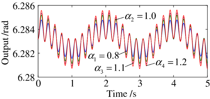
Output responses of system (37) to loading inputs of concern
The application of the NOFRFs-based evaluation to the applied loading inputs and corresponding output responses shown in Fig. 4 yields
$$ \overline{Y}_{0} \left( {0} \right) = 6.2831 \approx 2\pi $$indicating the equilibrium associated with the considered system operating condition is.
\(x_{0} = 2\pi\).
-
Step 3 The standardized model of the system is therefore obtained as
$$ mr\ddot{\overline{x}}\left( t \right) + mg\sin \left[ {\overline{x}\left( t \right)} \right] = f\left( t \right) $$(38)where \(\overline{x}\left( t \right) = x\left( t \right) - 2\pi\). Apply the polynomial expansion
$$ \sin \left[ {\overline{x}\left( t \right)} \right] = \overline{x}\left( t \right) + \frac{ - 1}{{3!}}\overline{x}^{3} \left( t \right) + \frac{1}{5!}\overline{x}^{5} \left( t \right) + \cdots $$(39)up to the fifth order, the standardized model (38) can then be represented in the form of NDE model (10) as
$$ mr\ddot{\overline{x}}\left( t \right) + mg\left( {\overline{x}\left( t \right) + \frac{ - 1}{{3!}}\overline{x}^{3} \left( t \right) + \frac{1}{5!}\overline{x}^{5} \left( t \right)} \right) = f\left( t \right) $$(40)In the following, three case studies will be used to demonstrate the application of the proposed nonlinear model standardization to address different engineering problems.

5 Case studies
5.1 Case study 1–Application to the detection of cracks in beam structures
The detection of cracks in beam structures has been widely investigated by researchers [38, 39]. A NOFRFs-based approach to the detection of cracks in beams has recently been proposed to exploit nonlinearities induced by cracks to find locations [35, 36] and to evaluate severities [21, 40] of cracks in beam structures. It has been demonstrated that, compared to traditional crack detections using system output spectra, the NOFRFs-based indices are more sensitive to crack defects [21, 40].
There are two different experimental setups for the detection of cracks in a beam which, as shown in Fig. 5, are (a) vertical setup and (b) horizontal setup, respectively. In previous studies [35], both setups were used but the effects of gravity on the analysis were ignored. This is acceptable in some cases, but for beams with a large length–width ratio and small stiffness, the gravity effects may change the operating point of the system and significantly affect the analysis and hence the results of crack detection [41]. In this case study, the proposed nonlinear model standardization method is applied to take the effects of gravity of a beam structure into account and the NOFRFs based approach is then used to detect cracks in the beam. The objective is to demonstrate how to apply the proposed nonlinear model standardization to resolve a significant structural integrity evaluation problem.

Experimental setup for detection of cracks in beams. a Vertical setup; b Horizontal setup
Under vertical setup as shown in Fig. 5a, the effects of gravity \(G\) can be ignored since it does not affect the horizontal vibration of the beam.
For example, consider a beam system represented by an NDE model as [21]
where \(\xi { = }0.2\), \(\omega_{0} = 120\pi \;{{{\text{rad}}} \mathord{\left/ {\vphantom {{{\text{rad}}} {\text{s}}}} \right. \kern-\nulldelimiterspace} {\text{s}}}\), and \(u\left( t \right) =\)\(\cos \left( {\omega_{F} t} \right)\) are the damping ratio, natural frequency, and input of the system, respectively. \(k_{n2}\) and \(k_{n4}\) are the parameters directly related to the crack characteristics in the beam with \(k_{n4} = 1 \times 10^{16}\) and \(k_{n2}\) varied over the range of \(k_{n2} =\)\(\left\{ {0:0.5:10} \right\} \times 10^{9}\) to represent different severities of cracks in the beam.
Obviously, (41) has zero equilibrium and is, therefore, already a standardised model. Consequently, the variation of the NOFRFs of the system with the changes of \(k_{n2}\) over the range of \(k_{n2} = \left\{ {0:0.5:10} \right\} \times 10^{9}\) can directly be determined from the system’s input output data using the algorithm in [21] to detect and quantify the severity of cracks in the beam. The results are as shown in Fig. 6.

Change of the NOFRFs with the increase in \(k_{n2}\)
Under horizontal setup as shown in Fig. 5b, however, the effects of gravity have to be considered and the beam system should be described as
where \(F_{{\text{G}}} = 0.88\) is the normalized beam gravity. Because the equilibrium of the beam system model (42) is not zero, the model has to be standardized first then the NOFRFs approach can be applied to the input output data of the standardized model for crack detection as shown in [21].
It is worth noting that the cracked beam models (41) and (42) are widely used to represent nonlinear dynamics in cracked beam structures known as the “second-order super-harmonics” [41].
For example, when \(k_{n2} = 2 \times 10^{8}\), following the three steps proposed in Sect. 4, the standardization of nonlinear model (42) is conducted as follows.
-
Step 1 Denote \(y\left( t \right) = \overline{y}\left( t \right) + y_{0}\). According to Proposition 1, model (42) can be standardized as
$$ \begin{gathered} \ddot{\bar{y}}\left( t \right) + \left( {1.421 \times 10^{5} + 4 \times 10^{8} y_{0} - 4 \times 10^{{16}} y_{0} ^{3} } \right)\bar{y}\left( t \right) \hfill \\ \quad \quad + 1.508 \times 10^{2} \dot{\bar{y}}\left( t \right) + \left( {2 \times 10^{8} - 6 \times 10^{{16}} y_{0} ^{2} } \right)\bar{y}^{2} \left( t \right) \hfill \\ \quad \quad - 4 \times 10^{{16}} y_{0} \bar{y}^{3} \left( t \right) - 1 \times 10^{{16}} \bar{y}^{4} \left( t \right) = u\left( t \right) \hfill \\ \end{gathered} $$(43)The equilibria \(y_{0,1} , \ldots ,y_{{0,N_{e} }}\) are evaluated by solving equation
$$ - 1 \times 10^{16} y_{0}^{4} + 2 \times 10^{8} y_{0}^{2} + 1.421 \times 10^{5} y_{0} - 0.88 = 0 $$(44)yielding \(N_{e} = 2\),
$$ y_{0,1} = 2.6797 \times 10^{ - 4} \;{\text{and}}\;y_{0,2} = 6.1389 \times 10^{ - 6} $$(45) -
Step 2 The output spectrum of the standardized model at zero frequency can be represented using the NOFRFs up to eighth order (\(N = 8\)) as
$$ Y\left( 0 \right) = \overline{y}_{0} + \sum\limits_{i = 1}^{4} {\overline{G}_{2i} \left( 0 \right)U_{2i} \left( 0 \right)} $$(46)where only even order NOFRFs are involved because the constraint \(\omega_{1} + \cdots + \omega_{n} = 0\) with \(\omega_{i} = \pm \omega_{F} ,\;i = 1, \ldots ,n\) should be satisfied [29].
Evaluating the NOFRFs and \(\overline{y}_{0}\) in (46) from the system responses to inputs \(u\left( t \right) = \alpha \cos \left( {\omega_{F} t} \right)\) with \(\alpha = \left\{ {0.8:0.1:\;1.2} \right\}\) and \(\omega_{F} = \omega_{0}\) yields
$$ \overline{y}_{0} = 6.1393 \times 10^{ - 6} $$(47)Step 3 By comparing the equilibria in (45) and the evaluated \(\overline{y}_{0}\) in (47), the stable equilibrium associated with the system operating condition represented by input \(u\left( t \right) = \cos \left( {\omega_{F} t} \right)\) is found to be \(y_{0} = y_{0,2} = 6.1389\)\(\times 10^{ - 6} \approx \overline{y}_{0}\). Thus substituting \(y_{0} = y_{0,2} = 6.1389 \times 10^{ - 6}\) into (45) yields the standardized nonlinear model
$$ \begin{gathered} \ddot{\bar{y}}\left( t \right) + 1.508 \times 10^{2} \dot{\bar{y}}\left( t \right) + 1.3962 \times 10^{5} \bar{y}\left( t \right) \hfill \\ \quad \quad - 3.4375 \times 10^{7} \bar{y}^{2} \left( t \right) - 2.5 \times 10^{{12}} \bar{y}^{3} \left( t \right) \hfill \\ \quad \quad - 1 \times 10^{{16}} \bar{y}^{4} \left( t \right) = u\left( t \right) \hfill \\ \end{gathered} $$(48)Repeating Step 1 to Step 3 for \(k_{n2} = \left\{ {0:0.5:10} \right\} \times 10^{9}\), respectively, produce 21 standardized nonlinear models of the beam in the case of horizontal setup under 21 different crack severities. The NOFRFs of the standardized models, denoted as \(\overline{G}_{n} \left( {{\text{j}}\omega } \right)\) are then evaluated using the algorithm proposed in [21] from the input and output data of the standardized model (48). The results are also shown in Fig. 6.
When the cantilever beam is tested under vertical setup, the gravity does not need to be considered and the model is already standardized. In this case, the second order NOFRF magnitude \(\left| {G_{2} \left( {{\text{j2}}\omega_{F} } \right)} \right|\) increase linearly and monotonously with the increase in \(k_{n2}\) and the magnitude of the first order NOFRF \(\left| {G_{1} \left( {{\text{j}}\omega_{{\text{F}}} } \right)} \right|\) is a constant. When the cantilever beam is tested under horizontal setup, however, the gravity can significantly change the profile of the NOFRFs: the magnitude of the first order NOFRF \(\left| {\overline{G}_{1} \left( {{\text{j}}\omega_{F} } \right)} \right|\) monotonously decreases with the increase in \(k_{n2}\), but the magnitude of the second order NOFRF \(\left| {\overline{G}_{2} \left( {{\text{j2}}\omega_{F} } \right)} \right|\) is almost a constant when \(k_{n2}\) increases. These observations indicate that the second order NOFRF should be used for the detection and quantification of cracks when the cantilever beam is tested under vertical setup, while the first-order NOFRF should be used when the cantilever beam is tested under horizontal setup. In addition, the results also show that when beams are tested under horizontal setup, the proposed nonlinear model standardization is necessary for the application of the NOFRFs approach to the detection of cracks.
Traditional solution to the problems relevant to this case study is to find all possible equilibria of the system in (45) and then select one of them of concern for the study. This, however, cannot address the issue with how to determine the equilibrium associated with the operational condition when a system is working under a specific input. This case study demonstrates that the proposed NOFRFs based approach can directly determine the operating point of interest of a beam structure and produce a standardized model to facilitate the detection of cracks in the beam.
5.2 Case study 2–Application to the design of an Auxetic foam structure
Auxetic foams are made of materials of negative Poisson’s ratio and can be used to significantly dissipate vibration energy [41, 49]. In [42], a NARX model with parameters of interest for the design of an Auxetic foam structure was identified based on the experimental data under sampling frequency \(f_{s} = 100\;{\text{Hz}}\) as
where \(y\left( k \right)\) and \(f\left( k \right)\) represent the input displacement (mm) and the output force (N), respectively. \(A\) and \(V\) are the design parameters representing the axial and volume ratio of the foam, and \(\theta_{m} \left( {A,V} \right)\), \(m = 1, \ldots ,8\) are polynomial functions of \(A\) and \(V\) with their values under 4 different pairs of \(A\) and \(V\) shown in Table 1 in Appendix 2.
Due to vibration energy dissipation properties, Auxetic foam can be used in a vibration isolation system as shown in Fig. 7, where \(u\left( t \right)\) is the force input, \(y\left( t \right)\) is the displacement output, and \(f_{{{\text{out}}}} \left( t \right)\) represents the force transmitted to the ground.

Auxetic foam structure-based vibration isolation system
The dynamic model of the isolation system in Fig. 7 is given by
where in this case study, \(m = 5\;{\text{kg}}\) and \(g = 9.8\;{{\text{m}} \mathord{\left/ {\vphantom {{\text{m}} {{\text{s}}^{{2}} }}} \right. \kern-\nulldelimiterspace} {{\text{s}}^{{2}} }}\).
The NDE model (50) can be discretized to produce a NARX model
by substituting the central difference [4]
and (49) into (50) with \(\Delta t = {1 \mathord{\left/ {\vphantom {1 {f_{s} }}} \right. \kern-\nulldelimiterspace} {f_{s} }} = 0.01\;{\text{s}}\).
Now, consider design of the manufacturing parameters \(\left( {A,\;V} \right)\) of the foam structure when the vibration isolation system is subject to the harmonic loading \(u\left( t \right) = F_{0} \cos \left( {\omega_{F} t} \right)\) where \(F_{0} = 5\;{\text{N}}\) and \(\omega_{F} = 120\;{{{\text{rad}}} \mathord{\left/ {\vphantom {{{\text{rad}}} {\text{s}}}} \right. \kern-\nulldelimiterspace} {\text{s}}}\). In order to conduct the design, as the first step, the standardized model (51) about a stable operating equilibrium should be built. The proposed nonlinear model standardization is, therefore, applied to model (51) of the isolation system following the three standardization steps in Sect. 4 as follows.
-
Step 1 Denote \(y\left( k \right) = \overline{y}\left( k \right) + y_{{0}}\) and use Proposition 1 to write the standardized model of system (51) as
$$ \begin{aligned} \overline{y}\left( k \right) = & 2\overline{y}\left( {k - 1} \right) - \overline{y}\left( {k - 2} \right) \\ \quad & - \frac{{\Delta t^{2} }}{m}f_{0} \left( {k - 1} \right) + \frac{{\Delta t^{2} }}{m}u\left( {k - 1} \right) \\ \end{aligned} $$(53)where
$$ \begin{aligned} f_{0} \left( k \right) = & \theta_{1} \left( {A,V} \right)\overline{y}^{2} \left( k \right) + \theta_{3} \left( {A,V} \right)\overline{y}\left( {k - 1} \right)\overline{y}\left( {k - 3} \right) \\ \quad & + \left[ {\theta_{2} \left( {A,V} \right) + y_{{0}} \theta_{3} \left( {A,V} \right) + y_{{0}} \theta_{8} \left( {A,V} \right)} \right]\overline{y}\left( {k - 1} \right) \\ \quad & + \theta_{4} \left( {A,V} \right)\overline{y}^{2} \left( {k - 3} \right) + \theta_{5} \left( {A,V} \right)\overline{y}\left( {k - 2} \right) \\ \quad & + \left[ {2y_{{0}} \theta_{1} \left( {A,V} \right) + \theta_{6} \left( {A,V} \right) + y_{{0}} \theta_{8} \left( {A,V} \right)} \right]\overline{y}\left( k \right) \\ \quad & + \left[ {y_{{0}} \theta_{3} \left( {A,V} \right) + 2y_{{0}} \theta_{4} \left( {A,V} \right)} \right]\overline{y}\left( {k - 3} \right) \\ \quad & + \theta_{8} \left( {A,V} \right)\overline{y}\left( k \right)\overline{y}\left( {k - 1} \right) \\ \end{aligned} $$(54)The equilibria of system (51) can be found from the solutions to equation
$$ \begin{gathered} \left[ {\theta_{1} \left( {A,V} \right) + \theta_{3} \left( {A,V} \right) + \theta_{4} \left( {A,V} \right) + \theta_{8} \left( {A,V} \right)} \right]y_{{0}}^{2} \hfill \\ \;\;\;\; + \left[ {\theta_{2} \left( {A,V} \right) + \theta_{5} \left( {A,V} \right) + \theta_{6} \left( {A,V} \right)} \right]y_{{0}} \hfill \\ \;\;\;\; + \theta_{7} \left( {A,V} \right) + mg = 0 \hfill \\ \end{gathered} $$(55)The results of the solutions under different sets of design parameters are shown in Table 2, indicating that, for each set of design parameters, there are two equilibria with the nonlinear vibration isolation system.
Table 2 Zero-order NOFRF under different design parameters -
Step 2 The NOFRFs representation of the output spectrum of system (51) at zero frequency can be written as
$$ Y\left( 0 \right) = \overline{y}_{0} + \sum\limits_{i = 1}^{4} {\overline{G}_{2i} \left( 0 \right)U_{2i} \left( 0 \right)} $$(56)when \(N = 8\). From the responses of system (51) to 5 different inputs.
\(u\left( k \right) = 5\alpha \cos \left( {120k\Delta t} \right),\;\alpha = \left\{ {0.8,\;0.9,\;1.0,\;1.1,\;1.2} \right\}\). (57).
around the operating condition represented by \(u\left( k \right) =\) \(5\cos \left( {120k\Delta t} \right)\), the equilibrium \(\overline{y}_{0}\) corresponding to this operating condition is determined following Step 2 in Sect. 4.2. The results under four different sets of design parameters are shown in Table 3.
Table 3 \(\theta_{{\text{m}}} \left( {A,V} \right)\) under different parameters of A and V Comparing the results in Tables. 2 and 3 shows that the equilibrium of concern for the design is \(\overline{y}_{0} \approx y_{{{0},1}}\).
-
Step 3 Substituting \(y_{0} = y_{{{0},1}}\) into (54), yields
$$ \begin{aligned} f_{0} \left( k \right) = & \overline{\theta }_{1} \left( {A,V} \right)\overline{y}^{2} \left( k \right) + \overline{\theta }_{2} \left( {A,V} \right)\overline{y}\left( {k - 1} \right) \\ \quad & + \overline{\theta }_{3} \left( {A,V} \right)\overline{y}\left( {k - 1} \right)\overline{y}\left( {k - 3} \right) + \overline{\theta }_{4} \left( {A,V} \right)\overline{y}^{2} \left( {k - 3} \right) \\ \quad & + \overline{\theta }_{5} \left( {A,V} \right)\overline{y}\left( {k - 2} \right) + \overline{\theta }_{6} \left( {A,V} \right)\overline{y}\left( k \right) \\ \quad & + \overline{\theta }_{7} \left( {A,V} \right)\overline{y}\left( {k - 3} \right) + \overline{\theta }_{8} \left( {A,V} \right)\overline{y}\left( k \right)\overline{y}\left( {k - 1} \right) \\ \end{aligned} $$(58)where \(\overline{\theta }_{{\text{i}}} \left( {A,V} \right).,i = 1,...,8\) are as shown in Table 4 in Appendix 2. Thus, the standardized nonlinear model for the Auxetic foam structure-based vibration isolation system is now obtained and given by Eqs. (53) and (58)
Table 4 \(\overline{\theta }_{{\text{m}}} \left( {A,V} \right)\) under different parameter of A and V Assume that the design is to achieve a vibration isolation performance defined by the force transmissibility
$$ T\left( {{\text{j}}\omega } \right) = \frac{{F_{out} \left( {{\text{j}}\omega } \right)}}{{U\left( {{\text{j}}\omega } \right)}} $$(59)where \(F_{{{\text{out}}}} \left( {{\text{j}}\omega } \right)\) is the Fourier Transform of the output force \(f_{{{\text{out}}}} \left( t \right)\), the design problem can be formulated as follows:
Find \(\left( {A,V} \right)\), such that
$$ \left| {T\left( {{\text{j}}120} \right)} \right| \le 2 $$(60)under the constraint of.
$$ A \in \left[ {1.13,\;2.13} \right]\;{\text{and}}\;V = 2.485A $$(61)In this design problem, constraint (61) shows that \(A\) and \(V\) are linear correlated so that only one of the two parameters need to be used for the design. Considering \(T\left( {{\text{j}}\omega } \right)\) with \(\omega \ne 0\), there is
$$ \begin{aligned} T\left( {{\text{j}}\omega } \right) = & \frac{{FT\left[ {f_{out} \left( t \right)} \right]}}{{U\left( {{\text{j}}\omega } \right)}} = \frac{{FT\left[ {u\left( t \right) + mg - m\ddot{y}\left( t \right)} \right]}}{{U\left( {{\text{j}}\omega } \right)}} \\ = & 1 - \frac{{m\left( {{\text{j}}\omega } \right)^{2} }}{{U\left( {{\text{j}}\omega } \right)}}Y\left( {{\text{j}}\omega } \right) = 1 + \frac{{m\omega^{2} }}{{U\left( {{\text{j}}\omega } \right)}}\overline{Y}\left( {{\text{j}}\omega } \right) \\ \end{aligned} $$(62)where \(FT\left[ . \right]\) represents the Fourier Transform. Moreover, considering \(\overline{\theta }_{m} \left( {A,V} \right)\), \(m = 1, \ldots ,8\) can be represented as polynomial functions of \(A\) by data fitting using the results in Table 4 in Appendix 2, both \(\overline{Y}\left( {{\text{j}}\omega } \right)\) and \(T\left( {{\text{j}}\omega } \right)\) can be described, using the associated output frequency response function (AOFRF) approach proposed in [43] as a complex valued polynomial function of \(A\) with the coefficients of the polynomial being dependent on both frequency variable \(\omega\) and the system input.
For example, a third-order AOFRF representation of the force transmissibility \(T\left( {{\text{j}}\omega } \right)\) at \(\omega = 120\;{{{\text{rad}}} \mathord{\left/ {\vphantom {{{\text{rad}}} {\text{s}}}} \right. \kern-\nulldelimiterspace} {\text{s}}}\) can be obtained using Eq. (62) by evaluating the AOFRF representation of the standardized model output spectrum \(\overline{Y}\left( {{\text{j}}\omega } \right)\) as
$$ \begin{aligned} T\left( {{\text{j}}120} \right) = & \left( { - 6.574 + 7.614{\text{i}}} \right) + \left( {11.553 - 14.391{\text{i}}} \right)A \\ \quad & + \left( { - 6.014 + 10.715{\text{i}}} \right)A^{2} + \left( {0.786 - 2.389{\text{i}}} \right)A^{3} \\ \end{aligned} $$(63)From (63), how \(\left| {T\left( {{\text{j}}120} \right)} \right|\) varies with the changes of \(A\) can be determined. The result is shown in Fig. 8. Figure 8 shows that a solution to the optimization problem (60) and (61) can be found as
$$ A = 1.45,\;V = 3.60 $$(64)Fig. 8 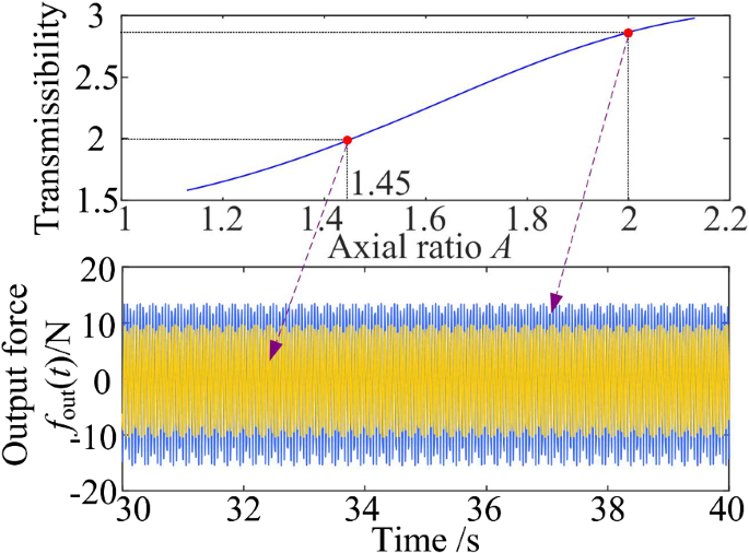
AOFRF representation of the force transmissibility and the output forces under the optimal and a different design
A comparison of the output force under the optimal design and the output force under \(\left( {A,V} \right) = \left( {2.00,4.97} \right)\), a different choice of the design parameters, is also shown in Fig. 8, indicating that the system under the optimal design does perform better.

This case study demonstrates how the operating point of the Auxetic foam-based vibration isolation system is evaluated using the NOFRFs approach, based on which the standardized model of the system can be determined for the analysis and design. Again, this is difficult to be achieved using the traditional method by simply finding all possible equilibria.
5.3 Case study 3–Application to the compensation for system nonlinearity
Compensation for system nonlinearity has been widely considered in electrical and optical communication systems [19, 44] including, for example, the compensation for pre-distortion in the radio frequency power amplifier in wireless communication systems [19]. The purpose of the nonlinearity compensation is to eliminate the unwanted nonlinear effects of a system on signals passing through the system [44], so that original signals can correctly be restored from the system outputs. The Volterra series approach is one of the most powerful techniques in nonlinearity compensation [45], by which, nonlinear distortions can be reduced by using a cascaded inverse system as shown in Fig. 9a. In Fig. 9a, \({\text{H}}\) represents the nonlinear system that induces nonlinear distortions on input signal \(u\left( k \right)\), and \({\text{Q}}\) is the inverse of system \({\text{H}}\) that can be determined using the Volterra series approach and used to compensate for the nonlinear distortions [46].

An illustration of compensation for system nonlinearity, where a Compensation for system nonlinearity around zero stable equilibrium, and b Compensation for system nonlinearity around nonzero equilibrium
If nonlinear system \({\text{H}}\) is stable at zero equilibrium, its inverse system \({\text{Q}}\) can be determined by first determining the GFRFs \(H_{n} \left( {\omega_{1} ,\; \cdots ,\omega_{n} } \right),\;n = 1, \ldots ,N\) of system \({\text{H}}\) from the algorithm in Appendix 1a and then finding the corresponding inverse of \(H_{n} \left( {\omega_{1} ,\; \cdots ,\omega_{n} } \right),\;n = 1, \ldots ,N\) from [47]. The basic principle can be summarized as follows.
The output spectrum of system H in Fig. 9a can be represented by the Volterra series using (5) as
and the output spectrum of the compensating system \({\text{Q}}\) can be represented as
Substituting (65) into (66) yields
For the purpose of compensating for system nonlinearities, in (67), letting all higher order terms of \(U\left( {{\text{j}}\omega } \right)\) be zeros yields
so that the compensating system \({\text{Q}}\) can be determined by solving (68) for \(Q_{n} \left( {\omega_{1} ,\; \cdots ,\omega_{n} } \right),\;n = 1, \ldots ,N\).
However, when nonlinear system H has several stable equilibria, before the procedure above can be applied, the model of the nonlinear system needs to be standardized about the equilibrium associated with the input signal to be processed. The standardization involves, as shown in Fig. 9b, determining the system stable equilibrium associated with the input signal to process, and evaluating the GFRFs of the compensating system Q corresponding to the determined equilibrium. In the following, the nonlinear model standardization will be applied to system (2) to demonstrate how to apply the proposed nonlinear model standardization to address the problem of compensation for the nonlinearities in the system over two different stable equilibria, which are \(y_{0} = y_{0,3} = 1\) and \(y_{0} = y_{0,1} = - 1\), respectively. In case (ii) of system (2) and under the operating condition (a) where \(u\left( k \right) = 0.1\cos \left( {20k\Delta t + \varphi } \right)\) with \(\varphi = 0\), the standardized model can be obtained, using the proposed method, as given by Eq. (36) with \(y_{0} = y_{0,3} = 1\). Under the operating condition (b) where \(u\left( k \right) =\) \(0.1\cos \left( {20k\Delta t + \varphi } \right)\) with \(\varphi = \pi\), the standardized model can be obtained in the same way as
where \(y_{0} = y_{0,1} = - 1\).
Under operating condition (a), the standardized model (36) needs to be used for compensation for the system nonlinearity following the procedure proposed in [43] as briefly introduced above and illustrated in Fig. 9b while under operating condition (b) the standardized model (69) needs to be used instead.
It is worth noting that the compensated result can be significantly distorted if a wrong standardized model is used. For example, under operating condition (a) where \(u\left( k \right) =\) \(0.1\cos \left( {20k\Delta t} \right)\), the correct standardized model is (36) and the system’s first and second order GFRFs can be determined from (36) as
The GFRFs of the corresponding compensating system \({\text{Q}}\) can then be determined as
Consequently, the compensated signal \(z\left( k \right)\) can be obtained from the inverse Fourier transform of its spectrum
as shown in Fig. 10.

Compensation for nonlinearity of system (2) about equilibrium \(y_{0} = y_{0,3} = 1\) using correct standardized model (36)
Figure 10 shows that the nonlinear distortion induced by system (2) can be well compensated by using the inverse of the standardized model (36), producing a compensated signal such that \(z\left( k \right) = u\left( k \right)\). However, if the standardized model under the given operational condition is wrongly chosen as model (69), the compensated signal will be significantly distorted in both amplitude and phase as shown in Fig. 11. These results demonstrate the important role of the proposed nonlinear model standardization for the compensation for system nonlinearity, which has applications in many engineering systems.

Compensation for nonlinearity of system (2) about equilibrium \(y_{0} = y_{0,1} = - 1\) using incorrect standardized model (69)
It is worth noting that there are many approaches that can be used to study nonlinear compensation, and most of these approaches were developed based on the Volterra series representation [44,45,46, 48]. However, none of these studies have tried to discuss the multi-equilibria issue as these approaches are mainly focused on nonlinearity compensation around a known stable equilibrium [24, 25]. This case study raises the possible multi-equilibria problem with nonlinearity compensation and demonstrates how to apply the proposed approach to resolve this issue.
6 Conclusions
Linearization has been widely applied to study nonlinear systems over a small range about a stable equilibrium. In order to conduct the analysis, design and control of nonlinear systems over a wider range of operation, the Volterra series theory of nonlinear systems is often applied. This needs to transform the original model of nonlinear systems into a form that can be studied using the Volterra series approach. This transformation is referred to as nonlinear model standardization which can be considered to be an extension of the concept of linearization. In the present study, a novel and systematic approach has been developed to conduct the model standardization for nonlinear systems that can be represented by a NARX/NDE model of nonlinear systems. The approach involves the evaluation of the system’s stable equilibrium under the operating condition of interest, and the determination of a standardized nonlinear model about this equilibrium.
The results extend the well-known linearization concept to the nonlinear case to produce a nonlinear model about a stable equilibrium of concern such that the Volterra series and associated approaches for nonlinear systems can be applied for the system analysis and design.
Three case studies have been used to show how to apply the proposed nonlinear model standardization to address different engineering problems including the detection of cracks in beams, the design of Auxetic foam structure for vibration isolation, and compensation for system nonlinearities. These demonstrate the significance of the proposed nonlinear model standardization in a wide range of engineering practices.
References
Callier, F.M., Desoer, C.A.: Linear system theory. Springer Science & Business Media, Berlin (2012)
Liu, X., Yu, X., Zhou, X., Xi, H.: Finite-time H_ infinity control for linear systems with semi-Markovian switching. Nonlinear Dyn. 85, 2297–2308 (2016)
Roy, D.: Explorations of the phase-space linearization method for deterministic and stochastic nonlinear dynamical systems. Nonlinear Dyn. 23, 225–258 (2000)
Zhu, Y., Lang, Z.Q.: Design of nonlinear systems in the frequency domain: an output frequency response function-based approach. IEEE Trans. Control Syst. Technol. 26, 1358–1371 (2017)
Motsa, S.S., Sibanda, P.: A multistage linearisation approach to a four-dimensional hyperchaotic system with cubic nonlinearity. Nonlinear Dyn. 70, 651–657 (2012)
Tien, M.H., D’Souza, K.: A generalized bilinear amplitude and frequency approximation for piecewise-linear nonlinear systems with gaps or prestress. Nonlinear Dyn. 88, 2403–2416 (2017)
Tahmasian, S., Katrahmani, A.: Vibrational control of mechanical systems with piecewise linear damping and high-frequency inputs. Nonlinear Dyn. 99, 1403–1413 (2020)
Wredenhagen, G.F., Belanger, P.R.: Piecewise-linear LQ control for systems with input constraints. Automatica 30, 403–416 (1994)
Tapia, A., Bernal, M., Fridman, L.: An LMI approach for second-order sliding set design using piecewise Lyapunov functions. Automatica 79, 61–64 (2017)
George, D. A.: Continuous nonlinear systems. (No. TR-355),” Massachusetts Inst of Tech Cambridge Research Lab of Electronics, (1959).
Rugh, W.J.: Nonlinear system theory, pp. 12–90. Johns Hopkins University Press, Baltimore, MD (1981)
Chung, K.W., Chan, C.L., Xu, Z., Mahmoud, G.M.: A perturbation-incremental method for strongly nonlinear autonomous oscillators with many degrees of freedom. Nonlinear Dyn. 28, 243–259 (2002)
Doyle, F.J., Pearson, R.K., Ogunnaike, B.A.: Identification and control using Volterra models. Springer, London (2002)
Worden, K.: Nonlinearity in structural dynamics: detection, identification and modelling. CRC Press (2019)
Teixeira, M.C., Zak, S.H.: Stabilizing controller design for uncertain nonlinear systems using fuzzy models. IEEE Trans. Fuzzy Syst. 7, 133–142 (1999)
Goldgeisser, L.B., Green, M.M.: A method for automatically finding multiple operating points in nonlinear circuits. IEEE Trans. Circuits Syst. 52, 776–784 (2005)
Lang, Z.Q., Billings, S.A.: Output frequency characteristics of nonlinear systems. Int. J. Control. 64, 1049–1067 (1996)
Carassale, L., Kareem, A.: Modeling nonlinear systems by Volterra series. J. Eng. Mech. 136, 801–818 (2010)
Zhu, A., Pedro, J.C., Brazil, T.J.: Dynamic deviation reduction-based Volterra behavioral modeling of RF power amplifiers. IEEE Trans. Microw. Theory Tech. 54, 4323–4332 (2006)
Sekhar, A.S.: Multiple cracks effects and identification. Mech. Syst. Signal Process. 22(4), 845–878 (2008)
Bayma, R.S., Zhu, Y., Lang, Z.Q.: The analysis of nonlinear systems in the frequency domain using nonlinear output frequency response functions. Automatica 94, 452–457 (2018)
Mirri, D., Luculano, G., Filicori, F., Pasini, G., Vannini, G., Gabriella, G.P.: A modified Volterra series approach for nonlinear dynamic systems modelling. IEEE Trans. Circuits Syst. I-Fundam. Theor. Appl. 49, 1118–1128 (2002)
Huang, X., Liu, X., Hua, H.: On the characteristics of an ultra-low frequency nonlinear isolator using sliding beam as negative stiffness. J. Mech. Sci. Technol. 28, 813–822 (2014)
Feijoo, J.V., Worden, K., Rodríguez, N.J., Osorio, J.P., Ortiz, P.M.: Analysis and control of nonlinear systems with DC terms. Nonlinear Dyn. 58, 753 (2009)
Jones, J.P., Choudhary, K.: Efficient computation of higher order frequency response functions for nonlinear systems with, and without, a constant term. Int. J. Control. 85, 578–593 (2012)
Billings, S.A., Zhang, H.: Computation of non-linear transfer functions when constant terms are present. Mech. Syst. Signal Proc. 9, 537–553 (1995)
Jones, J.P., Billings, S.A.: Recursive algorithm for computing the frequency response of a class of non-linear difference equation models. Int. J. Control. 50, 1925–1940 (1989)
Billings, S.A., Peyton Jones, J.C.: Mapping non-linear integro-differential equations into the frequency domain. Int. J. Control. 52, 863–879 (1990)
Lang, Z.Q., Billings, S.A.: Energy transfer properties of non-linear systems in the frequency domain. Int. J. Control. 78, 345–362 (2005)
Thowsen, A.: The Routh-Hurwitz method for stability determination of linear differential-difference systems. Int. J. Control. 33, 991–995 (1981)
Bhatia, N.P., Szegö, G.P.: Stability theory of dynamical systems. Springer Science & Business Media, Berlin (2002)
Sastry, S.: Nonlinear systems: analysis, stability, and control, vol. 10. Springer Science & Business Media, Berlin (2013)
Aracil, J., Gordillo, F.: Describing function method for stability analysis of PD and PI fuzzy controllers. Fuzzy Sets Syst. 143, 233–249 (2004)
Sontag, E.D.: Smooth stabilization implies coprime factorization. IEEE Trans. Autom. Control. 34, 435–443 (1989)
Peng, Z.K., Lang, Z.Q., Billings, S.A.: Crack detection using nonlinear output frequency response functions. J. Sound Vibr. 301, 777–788 (2007)
Zhao, X.Y., Lang, Z.Q., Park, G., Farrar, C.R., Todd, M.D., Mao, Z., Worden, K.: A new transmissibility analysis method for detection and location of damage via nonlinear features in MDOF structural systems. IEEE-ASME Trans. Mechatron. 20, 1933–1947 (2014)
Yang, K., Zhang, Y.W., Ding, H., Chen, L.Q.: The transmissibility of nonlinear energy sink based on nonlinear output frequency-response functions. Commun. Nonlinear Sci. Numer. Simul. 44, 184–192 (2017)
Carden, E.P., Fanning, P.: Vibration based condition monitoring: a review. Struct. Health Monit. 3, 355–377 (2004)
Zeng, J., Ma, H., Zhang, W., Wen, B.: Dynamic characteristic analysis of cracked cantilever beams under different crack types. Eng. Fail. Anal. 74, 80–94 (2017)
Zhu, Y., Lang, Z. Q., Luo, Z., Gunawardena, S. R. A.: Fault Detection of Nonlinear Rotor Bearing Systems by Using the Nonlinear Output Frequency Response Functions (NOFRFs). In 2018 10th International Conference on Modelling, Identification and Control (ICMIC) (pp. 1–6). IEEE, (2018).
Ma, H., Zeng, J., Lang, Z., Zhang, L., Guo, Y., Wen, B.: Analysis of the dynamic characteristics of a slant-cracked cantilever beam. Mech. Syst. Signal Proc. 75, 261–279 (2016)
Wei, H.L., Lang, Z.Q., Billings, S.A.: Constructing an overall dynamical model for a system with changing design parameter properties. Int. J. Model. Ident. Control 5, 93–104 (2008)
Zhu, Y., Lang, Z.Q.: The effects of linear and nonlinear characteristic parameters on the output frequency responses of nonlinear systems: The associated output frequency response function. Automatica 93, 422–427 (2018)
Giacoumidis, E., Aldaya, I., Jarajreh, M.A., Tsokanos, A., Le, S.T., Farjady, F., Doran, N.J.: Volterra-based reconfigurable nonlinear equalizer for coherent OFDM. IEEE Photonics Technol. Lett. 26, 1383–1386 (2014)
Zhu, A., Draxler, P.J., Hsia, C., Brazil, T.J., Kimball, D.F., Asbeck, P.M.: Digital predistortion for envelope-tracking power amplifiers using decomposed piecewise Volterra series. IEEE Trans. Microw. Theory Tech. 56, 2237–2247 (2008)
Schoukens, J., Németh, J.G., Vandersteen, G., Pintelon, R., Crama, P.: Linearization of nonlinear dynamic systems. IEEE Trans. Instrum. Meas. 53, 1245–1248 (2004)
Schetzen, M.: Theory of pth-order inverses of nonlinear systems. IEEE Trans. Circuits Syst. 23, 285–291 (1976)
Morgan, D.R., Ma, Z., Kim, J., Zierdt, M.G., Pastalan, J.: A generalized memory polynomial model for digital predistortion of RF power amplifiers. IEEE Trans. Signal Process. 54, 3852–3860 (2006)
Scarpa, F.: Auxetic materials for bioprostheses [In the Spotlight]. IEEE Signal Process. Mag. 25, 128–126 (2008)
Acknowledgments
The author would like to acknowledge the support of the UK EPSRC for this research study.
Funding
UK EPSRC.
Author information
Authors and Affiliations
Corresponding author
Ethics declarations
Conflicts of interest
The authors declare that they have no conflict of interest.
Availability of data and material
Not available.
Code availability
Not available.
Appendices
Appendix 1
(a) The GFRFs \(H_{{\text{n}}} \left( {\omega_{1} ,\; \cdots ,\;\omega_{{\text{n}}} } \right)\) of the NARX model (1) can be evaluated by using algorithm [27]:
where
(b) The GFRFs \(\overline{H}_{n} \left( {\omega_{1} ,\; \cdots ,\;\omega_{n} } \right)\) of the NARX model with a constant term (5) can be evaluated by introducing \(H_{0}\) in algorithm (A1) and (A2) as [25]:
where \(H_{0}\) is determined from the equilibrium \(y_{0}\), and
Appendix 2
The parameters of the Auxetic foam structure model (49) and the standardized system model (53) under the constraint of \(V = 2.485A\) are shown in Tables 3 and 4, respectively,
Rights and permissions
Open Access This article is licensed under a Creative Commons Attribution 4.0 International License, which permits use, sharing, adaptation, distribution and reproduction in any medium or format, as long as you give appropriate credit to the original author(s) and the source, provide a link to the Creative Commons licence, and indicate if changes were made. The images or other third party material in this article are included in the article's Creative Commons licence, unless indicated otherwise in a credit line to the material. If material is not included in the article's Creative Commons licence and your intended use is not permitted by statutory regulation or exceeds the permitted use, you will need to obtain permission directly from the copyright holder. To view a copy of this licence, visit http://creativecommons.org/licenses/by/4.0/.
About this article

Cite this article
Zhu, YP., Lang, Z.Q. & Guo, YZ. Nonlinear model standardization for the analysis and design of nonlinear systems with multiple equilibria. Nonlinear Dyn 104, 2553–2571 (2021). https://doi.org/10.1007/s11071-021-06429-9
Received:
Accepted:
Published:
Issue Date:
DOI: https://doi.org/10.1007/s11071-021-06429-9