OGY-based control of chaos in semi-passive dynamic walking of a torso-driven biped robot

Abstract

This paper aims at controlling chaos exhibited in the semi-passive dynamic walking of a torso-driven biped robot as it goes down an inclined surface. Our control approach is based on the OGY method. The proposed biped robot is a three-degrees-of-freedom planar biped having an impulsive hybrid nonlinear dynamics. For this walker, we use only one torque between the stance leg and the torso in order to control the torso at some desired position and then in order to generate a semi-passive gait. The desired torso angle is considered as the control parameter in our OGY-based control approach. We develop a reduced simple impulsive hybrid linear model by linearizing the impulsive hybrid nonlinear dynamics around a desired period-1 hybrid limit cycle. This conducts to determine an explicit expression of a constrained controlled Poincaré map. A linearization of the controlled Poincaré map around its fixed point permits to looking for the gain matrix of the stabilizing control law. We show that application of the developed OGY-based control parameter law has controlled the chaotic semi-passive gait.

Appendices

Appendix 1

In this appendix, we determine expressions that give numerically the fixed point $\varvec{x}_{*}^{-}$ of the constrained controlled Poincaré map (33). According to [34], the fixed point $\varvec{x}_{*}^{-}$ must verify:

$$\begin{aligned} \left\{ \begin{array}{l} {\mathcal L}_{0}\left( \varvec{x}_{*}^{-}, \hat{\tau }_{*}, \theta ^{d}_{t*}\right) = \varvec{\mathcal {P}}\left( \varvec{x}_{*}^{-}, \hat{\tau }_{*}, \theta ^{d}_{t*}\right) - \varvec{x}_{*}^{-} = \varvec{0}\\ {\mathcal L}_{1}\left( \varvec{\mathcal {P}}\left( \varvec{x}_{*}^{-}, \hat{\tau }_{*}, \theta ^{d}_{t*} \right) \right) = 0\\ {\mathcal L}_{2}\left( \varvec{\mathcal {P}}\left( \varvec{x}_{*}^{-}, \hat{\tau }_{*}, \theta ^{d}_{t*} \right) \right) < 0 \\ {\mathcal L}_{3}\left( \varvec{\mathcal {P}}\left( \varvec{x}_{*}^{-}, \hat{\tau }_{*}, \theta ^{d}_{t*} \right) \right) > 0 \end{array}\right. . \end{aligned}$$

(37)

The two inequalities in (37) can be transformed to equalities as follows:

$$\begin{aligned} \left\{ \begin{array}{l} \hat{{\mathcal L}}_{2}\left( \varvec{x}_{*}^{-}, \hat{\tau }_{*}, \theta ^{d}_{t*}, \mu _{*} \right) = {\mathcal L}_{2}\left( \varvec{\mathcal {P}}\left( \varvec{x}_{*}^{-}, \hat{\tau }_{*}, \theta ^{d}_{t*} \right) \right) + \mu _{*}^{2} = 0 \\ \hat{{\mathcal L}}_{3}\left( \varvec{x}_{*}^{-}, \hat{\tau }_{*}, \theta ^{d}_{t*}, \eta _{*} \right) = {\mathcal L}_{3}\left( \varvec{\mathcal {P}}\left( \varvec{x}_{*}^{-}, \hat{\tau }_{*}, \theta ^{d}_{t*} \right) \right) - \eta _{*}^{2} = 0 \end{array} \right. . \end{aligned}$$

(38)

where $\mu _{*}$ and $\eta _{*}$ are two scalar variables.

As the state vector $\varvec{x}_{*}^{-}$ is of dimension 6, and ${\mathcal L}_{1}$, $\hat{{\mathcal L}}_{2}$ and $\hat{{\mathcal L}}_{3}$ are scalar functions, then we have nine equations and nine unknown variables, namely $\varvec{x}_{*}^{-}, \hat{\tau }_{*}, \mu _{*}$ and $\eta _{*}$. Hence, we can solve such constraints using the well-known Newton–Raphson method. Posing $\hat{{\mathcal L}}_{1}\left( \varvec{x}_{*}^{-}, \hat{\tau }_{*}, \theta ^{d}_{t*}\right) = {\mathcal L}_{1}\left( \varvec{\mathcal {P}}\left( \varvec{x}_{*}^{-}, \hat{\tau }_{*}, \theta ^{d}_{t*} \right) \right)$. Therefore, the fixed point $\varvec{x}_{*}^{-}$ is the solution of:

$$\begin{aligned} \varvec{{\mathcal L}}_{*}\left( \varvec{z}_{*}\right) = \left[ \begin{array}{c} {\mathcal L}_{0}\left( \varvec{x}_{*}^{-}, \hat{\tau }_{*}, \theta ^{d}_{t*}\right) \\ \hat{{\mathcal L}}_{1}\left( \varvec{x}_{*}^{-}, \hat{\tau }_{*}, \theta ^{d}_{t*}\right) \\ \hat{{\mathcal L}}_{2}\left( \varvec{x}_{*}^{-}, \hat{\tau }_{*}, \theta ^{d}_{t*}, \mu _{*} \right) \\ \hat{{\mathcal L}}_{3}\left( \varvec{x}_{*}^{-}, \hat{\tau }_{*}, \theta ^{d}_{t*}, \eta _{*} \right) \end{array}\right] = \varvec{0}, \end{aligned}$$

(39)

with $\varvec{z}_{*} = \left[ \begin{array}{c} \varvec{x}_{*}^{-}\\ \hat{\tau }_{*}\\ \mu _{*}\\ \eta _{*} \end{array} \right] \in {\mathcal {\mathfrak {R}}}^{9\times 1}$, and $\varvec{{\mathcal L}}_{*}\in {\mathcal {\mathfrak {R}}}^{9\times 1}$.

Appendix 2

This second appendix gives expressions of the state matrix ${\mathcal D}\varvec{\mathcal P}_{\varvec{x}_{k}^{-}}$ and the input matrix ${\mathcal D}\varvec{\mathcal P}_{\theta ^{d}_{tk}}$ of the linearized controlled Poincaré map (34) [34]. These two matrices are defined as follows:

$$\begin{aligned}&{\mathcal D}\varvec{\mathcal P}_{\varvec{x}_{k}^{-}} \left( \varvec{x}_{k}^{-}, \hat{\tau }_{k}, \theta ^{d}_{tk}\right) \nonumber \\&\quad = \frac{\partial \varvec{\mathcal P}\left( \varvec{x}_{k}^{-}, \hat{\tau }_{k}, \theta ^{d}_{tk}\right) }{\partial \varvec{x}_{k}^{-}} + \frac{\partial \varvec{\mathcal P}\left( \varvec{x}_{k}^{-}, \hat{\tau }_{k}, \theta ^{d}_{tk}\right) }{\partial \hat{\tau }_{k}}\frac{\partial \hat{\tau }_{k}}{\partial \varvec{x}_{k}^{-}}, \nonumber \\ \end{aligned}$$

(40)

$$\begin{aligned}&{\mathcal D}\varvec{\mathcal P}_{\theta ^{d}_{tk}} \left( \varvec{x}_{k}^{-}, \hat{\tau }_{k}, \theta ^{d}_{tk}\right) \nonumber \\&\quad = \frac{\partial \varvec{\mathcal P} \left( \varvec{x}_{k}^{-}, \hat{\tau }_{k}, \theta ^{d}_{tk}\right) }{\partial \theta ^{d}_{tk}} + \frac{\partial \varvec{\mathcal P}\left( \varvec{x}_{k}^{-}, \hat{\tau }_{k}, \theta ^{d}_{tk}\right) }{\partial \hat{\tau }_{k}}\frac{\partial \hat{\tau }_{k}}{\partial \theta ^{d}_{tk}}.\nonumber \\ \end{aligned}$$

(41)

In fact, determination of the matrices $\frac{\partial \varvec{\mathcal P}\left( \varvec{x}_{k}^{-}, \hat{\tau }_{k}, \theta ^{d}_{tk}\right) }{\partial \varvec{x}_{k}^{-}},$ $\frac{\partial \varvec{\mathcal P}\left( \varvec{x}_{k}^{-}, \hat{\tau }_{k}, \theta ^{d}_{tk}\right) }{\partial \theta ^{d}_{tk}}$ and $\frac{\partial \varvec{\mathcal P}\left( \varvec{x}_{k}^{-}, \hat{\tau }_{k}, \theta ^{d}_{tk}\right) }{\partial \hat{\tau }_{k}}$ is quite simple (see “Appendix 3”). However, determination of expression of the two quantities $\frac{\partial \hat{\tau }_{k}}{\partial \varvec{x}_{k}^{-}}$ and $\frac{\partial \hat{\tau }_{k}}{\partial \theta ^{d}_{tk}}$ requires the first impact constraint in (33): that is ${\mathcal L}_{1}\left( \varvec{\mathcal {P}}\left( \varvec{x}_{k}^{-}, \hat{\tau }_{k}, \theta ^{d}_{tk} \right) \right) =0$. Then, the derivative of this function with respect to $\varvec{x}_{k}^{-}$ yields:

$$\begin{aligned}&\frac{\partial {\mathcal L}_{1}\left( \varvec{\mathcal {P}} \left( \varvec{x}_{k}^{-}, \hat{\tau }_{k}, \theta ^{d}_{tk}\right) \right) }{\partial \varvec{x}_{k}^{-}} + \frac{\partial {\mathcal L}_{1}\left( \varvec{\mathcal {P}}\left( \varvec{x}_{k}^{-}, \hat{\tau }_{k}, \theta ^{d}_{tk}\right) \right) }{\partial \hat{\tau }_{k}}\mathrm{X} \nonumber \\&\quad \frac{\partial \hat{\tau }_{k}}{\partial \varvec{x}_{k}^{-}} = \varvec{0},\end{aligned}$$

(42)

$$\begin{aligned}&\frac{\partial {\mathcal L}_{1}\left( \varvec{\mathcal {P}} \left( \varvec{x}_{k}^{-}, \hat{\tau }_{k}, \theta ^{d}_{tk}\right) \right) }{\partial \theta ^{d}_{tk}} + \frac{\partial {\mathcal L}_{1}\left( \varvec{\mathcal {P}}\left( \varvec{x}_{k}^{-}, \hat{\tau }_{k}, \theta ^{d}_{tk}\right) \right) }{\partial \hat{\tau }_{k}} \mathrm{X}\nonumber \\&\quad \frac{\partial \hat{\tau }_{k}}{\partial \theta ^{d}_{tk}} = \varvec{0}. \end{aligned}$$

(43)

Relying on “Appendix 4” [expressions (63) and (64)], and using (42) and (43), we obtain expressions of the two quantities $\frac{\partial \hat{\tau }_{k}}{\partial \varvec{x}_{k}^{-}}$ and $\frac{\partial \hat{\tau }_{k}}{\partial \theta ^{d}_{tk}}$ like so:

$$\begin{aligned}&\frac{\partial \hat{\tau }_{k}}{\partial \varvec{x}_{k}^{-}} = - \frac{\frac{\partial {\mathcal L}_{1}\left( \varvec{\mathcal {P}}\left( \varvec{x}_{k}^{-}, \hat{\tau }_{k}, \theta ^{d}_{tk}\right) \right) }{\partial \varvec{\mathcal {P}}\left( \varvec{x}_{k}^{-}, \hat{\tau }_{k}, \theta ^{d}_{tk}\right) }\frac{\partial \varvec{\mathcal {P}}\left( \varvec{x}_{k}^{-}, \hat{\tau }_{k}, \theta ^{d}_{tk}\right) }{\partial \varvec{x}_{k}^{-}}}{{\mathcal L}_{2}\left( \varvec{\mathcal {P}}\left( \varvec{x}_{k}^{-}, \hat{\tau }_{k}, \theta ^{d}_{tk}\right) \right) }, \end{aligned}$$

(44)

$$\begin{aligned}&\frac{\partial \hat{\tau }_{k}}{\partial \theta ^{d}_{tk}} = - \frac{\frac{\partial {\mathcal L}_{1}\left( \varvec{\mathcal {P}}\left( \varvec{x}_{k}^{-}, \hat{\tau }_{k}, \theta ^{d}_{tk}\right) \right) }{\partial \varvec{\mathcal {P}}\left( \varvec{x}_{k}^{-}, \hat{\tau }_{k}, \theta ^{d}_{tk}\right) }\frac{\partial \varvec{\mathcal {P}}\left( \varvec{x}_{k}^{-}, \hat{\tau }_{k}, \theta ^{d}_{tk}\right) }{\partial \theta ^{d}_{tk}}}{{\mathcal L}_{2}\left( \varvec{\mathcal {P}}\left( \varvec{x}_{k}^{-}, \hat{\tau }_{k}, \theta ^{d}_{tk}\right) \right) }. \end{aligned}$$

(45)

We note that: $\frac{\partial {\mathcal L}_{1}\left( \varvec{\mathcal {P}}\left( \varvec{x}_{k}^{-}, \hat{\tau }_{k}, \theta ^{d}_{tk}\right) \right) }{\partial \varvec{\mathcal {P}}\left( \varvec{x}_{k}^{-}, \hat{\tau }_{k}, \theta ^{d}_{tk}\right) } = \frac{\partial {\mathcal L}_{1}\left( \varvec{x}_{k+1}^{-}\right) }{\partial \varvec{x}_{k+1}^{-}}$. Then, based on expression of ${\mathcal L}_{1}$ in (10), it follows that: $\frac{\partial {\mathcal L}_{1}\left( \varvec{\mathcal {P}}\left( \varvec{x}_{k}^{-}, \hat{\tau }_{k}, \theta ^{d}_{tk}\right) \right) }{\partial \varvec{\mathcal {P}}\left( \varvec{x}_{k}^{-}, \hat{\tau }_{k}, \theta ^{d}_{tk}\right) } = l\left( sin(\theta _{ns}+\varphi ) - sin(\theta _{s}+\varphi )\right)$.

Substituting the two expressions (44) and (45) into (40) and (41), respectively, expressions of the state matrix and the input matrix of the discrete linear system (34) are given as follows:

$$\begin{aligned}&{\mathcal D}\varvec{\mathcal P}_{\varvec{x}_{k}^{-}} \left( \varvec{x}_{k}^{-}, \hat{\tau }_{k}, \theta ^{d}_{tk}\right) \nonumber \\&\quad = \left[ \varvec{I}_{6} - \frac{\frac{\partial \varvec{\mathcal P}\left( \varvec{x}_{k}^{-}, \hat{\tau }_{k}, \theta ^{d}_{tk}\right) }{\partial \hat{\tau }_{k}}\frac{\partial {\mathcal L}_{1}\left( \varvec{\mathcal {P}}\left( \varvec{x}_{k}^{-}, \hat{\tau }_{k}, \theta ^{d}_{tk}\right) \right) }{\partial \varvec{\mathcal {P}}\left( \varvec{x}_{k}^{-}, \hat{\tau }_{k}, \theta ^{d}_{tk}\right) }}{{\mathcal L}_{2}\left( \varvec{\mathcal {P}}\left( \varvec{x}_{k}^{-}, \hat{\tau }_{k}, \theta ^{d}_{tk}\right) \right) }\right] \nonumber \\&\qquad \frac{\partial \varvec{\mathcal {P}}\left( \varvec{x}_{k}^{-}, \hat{\tau }_{k}, \theta ^{d}_{tk}\right) }{\partial \varvec{x}_{k}^{-}}, \end{aligned}$$

(46)

$$\begin{aligned}&{\mathcal D}\varvec{\mathcal P}_{\theta ^{d}_{tk}} \left( \varvec{x}_{k}^{-}, \hat{\tau }_{k}, \theta ^{d}_{tk}\right) \nonumber \\&\quad = \left[ \varvec{I}_{6} - \frac{\frac{\partial \varvec{\mathcal P}\left( \varvec{x}_{k}^{-}, \hat{\tau }_{k}, \theta ^{d}_{tk}\right) }{\partial \hat{\tau }_{k}}\frac{\partial {\mathcal L}_{1}\left( \varvec{\mathcal {P}}\left( \varvec{x}_{k}^{-}, \hat{\tau }_{k}, \theta ^{d}_{tk}\right) \right) }{\partial \varvec{\mathcal {P}}\left( \varvec{x}_{k}^{-}, \hat{\tau }_{k}, \theta ^{d}_{tk}\right) }}{{\mathcal L}_{2}\left( \varvec{\mathcal {P}}\left( \varvec{x}_{k}^{-}, \hat{\tau }_{k}, \theta ^{d}_{tk}\right) \right) }\right] \nonumber \\&\qquad \times \,\frac{\partial \varvec{\mathcal {P}}\left( \varvec{x}_{k}^{-}, \hat{\tau }_{k}, \theta ^{d}_{tk}\right) }{\partial \theta ^{d}_{tk}}. \end{aligned}$$

(47)

Appendix 3

In this third appendix, we define expressions of the matrices $\frac{\partial \varvec{\mathcal P}\left( \varvec{x}_{k}^{-}, \hat{\tau }_{k}, \theta ^{d}_{tk}\right) }{\partial \varvec{x}_{k}^{-}}$, $\frac{\partial \varvec{\mathcal P}\left( \varvec{x}_{k}^{-}, \hat{\tau }_{k}, \theta ^{d}_{tk}\right) }{\partial \theta ^{d}_{tk}}$ and $\frac{\partial \varvec{\mathcal P}\left( \varvec{x}_{k}^{-}, \hat{\tau }_{k}, \theta ^{d}_{tk}\right) }{\partial \hat{\tau }_{k}}$ in (40) and (41).

First, we recall that:

$$\begin{aligned}&\!\!\!\varvec{\mathcal {P}}\left( \varvec{x}_{k}^{-}, \hat{\tau }_{k}, \theta ^{d}_{tk} \right) = \varvec{\mathcal J}_{0}\left( \hat{\tau }_{k},\theta ^{d}_{tk}\right) \varvec{h} \left( \varvec{x}^{-}_{k}\right) \nonumber \\&\!\!\!\quad + \varvec{\mathcal H}_{0}\left( \hat{\tau }_{k}, \theta ^{d}_{tk}\right) , \end{aligned}$$

(48)

where

$$\begin{aligned} \varvec{\mathcal J}_{0}\left( \hat{\tau }_{k},\theta ^{d}_{tk}\right) =\varvec{\mathcal J}_{2}\left( \hat{\tau }_{k},\theta ^{d}_{tk}\right) \varvec{\mathcal J}_{1}\left( \theta ^{d}_{tk}\right) , \end{aligned}$$

(49)

and

$$\begin{aligned}&\!\!\!\varvec{\mathcal H}_{0}\left( \hat{\tau }_{k}, \theta ^{d}_{tk}\right) =\varvec{\mathcal J}_{2}\left( \hat{\tau }_{k},\theta ^{d}_{tk}\right) \varvec{\mathcal H}_{1}\left( \theta ^{d}_{tk}\right) \nonumber \\&\quad \!\!\!+\varvec{\mathcal H}_{2}\left( \hat{\tau }_{k}, \theta ^{d}_{tk}\right) . \end{aligned}$$

(50)

Moreover, we recall that:

$$\begin{aligned}&\varvec{\mathcal J}_{1}\left( \theta ^{d}_{tk}\right) = \prod _{i=1}^{n-1}\mathrm{e}^{\frac{\tau _{d}}{n}\varvec{A}_{i}}, \end{aligned}$$

(51)

$$\begin{aligned}&\varvec{\mathcal H}_{1}\left( \theta ^{d}_{tk}\right) = \sum _{i=1}^{n-1}\left( \prod _{j=i+1}^{n-1}\mathrm{e}^{\frac{\tau _{d}}{n} \varvec{A}_{j}}\right) \nonumber \\&\qquad \qquad \qquad \times \,\left( \mathrm{e}^{\frac{\tau _{d}}{n} \varvec{A}_{i}}-\varvec{\mathcal I}_{6}\right) \varvec{A}_{i}^{-1}\varvec{b}_{i}, \end{aligned}$$

(52)

$$\begin{aligned}&\varvec{\mathcal J}_{2}\left( \hat{\tau }_{k},\theta ^{d}_{tk}\right) = \mathrm{e}^{\hat{\tau }_{k}\varvec{A}_{n}},\end{aligned}$$

(53)

$$\begin{aligned}&\varvec{\mathcal H}_{2}\left( \hat{\tau }_{k}, \theta ^{d}_{tk}\right) = \left( \varvec{\mathcal J}_{2}\left( \hat{\tau }_{k},\theta ^{d}_{tk}\right) - \varvec{\mathcal I}_{6}\right) \varvec{A}_{n}^{-1} \varvec{b}_{n}, \end{aligned}$$

(54)

where, according to (21) and for $i=1,2,\ldots ,n$, we have:

$$\begin{aligned} \left\{ \begin{array}{rl} \varvec{A}_{i} &{} =\hat{\varvec{A}}_{i}+ \tilde{\varvec{A}}_{i}\theta ^{d}_{tk}\\ \varvec{b}_{i} &{} = \hat{\varvec{b}}_{i}+ \tilde{\varvec{b}}_{i}\theta ^{d}_{tk} \end{array}\right. \end{aligned}$$

(55)

Then, we deduce the following expressions:

• $\frac{\partial \varvec{\mathcal P}\left( \varvec{x}_{k}^{-}, \hat{\tau }_{k}, \theta ^{d}_{tk}\right) }{\partial \varvec{x}_{k}^{-}}=\varvec{\mathcal J}_{0}\left( \hat{\tau }_{k},\theta ^{d}_{tk}\right) \frac{\partial \varvec{h}\left( \varvec{x}^{-}_{k}\right) }{\partial \varvec{x}_{k}^{-}}$,

• $\frac{\partial \varvec{\mathcal P}\left( \varvec{x}_{k}^{-}, \hat{\tau }_{k}, \theta ^{d}_{tk}\right) }{\partial \hat{\tau }_{k}} = \frac{\partial \varvec{\mathcal J}_{0}\left( \hat{\tau }_{k},\theta ^{d}_{tk}\right) }{\partial \hat{\tau }_{k}}\varvec{h}\left( \varvec{x}^{-}_{k}\right) + \frac{\partial \varvec{\mathcal H}_{0}\left( \hat{\tau }_{k}, \theta ^{d}_{tk}\right) }{\partial \hat{\tau }_{k}}$,

• $\frac{\partial \varvec{\mathcal P}\left( \varvec{x}_{k}^{-}, \hat{\tau }_{k}, \theta ^{d}_{tk}\right) }{\partial \theta ^{d}_{tk}} = \frac{\partial \varvec{\mathcal J}_{0}\left( \hat{\tau }_{k},\theta ^{d}_{tk}\right) }{\partial \theta ^{d}_{tk}}\varvec{h}\left( \varvec{x}^{-}_{k}\right) + \frac{\partial \varvec{\mathcal H}_{0}\left( \hat{\tau }_{k}, \theta ^{d}_{tk}\right) }{\partial \theta ^{d}_{tk}}$,

• $\frac{\partial \varvec{\mathcal J}_{0}\left( \hat{\tau }_{k},\theta ^{d}_{tk}\right) }{\partial \hat{\tau }_{k}} = \frac{\partial \varvec{\mathcal J}_{2}\left( \hat{\tau }_{k},\theta ^{d}_{tk}\right) }{\partial \hat{\tau }_{k}}\varvec{\mathcal J}_{1}\left( \theta ^{d}_{tk}\right)$,

• $\frac{\partial \varvec{\mathcal H}_{0}\left( \hat{\tau }_{k}, \theta ^{d}_{tk}\right) }{\partial \hat{\tau }_{k}} = \frac{\partial \varvec{\mathcal J}_{2}\left( \hat{\tau }_{k},\theta ^{d}_{tk}\right) }{\partial \hat{\tau }_{k}}\varvec{\mathcal H}_{1}\left( \theta ^{d}_{tk}\right) + \frac{\partial \varvec{\mathcal H}_{2}\left( \hat{\tau }_{k},\theta ^{d}_{tk}\right) }{\partial \hat{\tau }_{k}}$,

• $\frac{\partial \varvec{\mathcal J}_{2}\left( \hat{\tau }_{k},\theta ^{d}_{tk}\right) }{\partial \hat{\tau }_{k}} = \varvec{A}_{n}\varvec{\mathcal J}_{2}\left( \hat{\tau }_{k},\theta ^{d}_{tk}\right)$,

• $\frac{\partial \varvec{\mathcal H}_{2}\left( \hat{\tau }_{k},\theta ^{d}_{tk}\right) }{\partial \hat{\tau }_{k}}\!=\!\frac{\partial \varvec{\mathcal J}_{2}\left( \hat{\tau }_{k},\theta ^{d}_{tk}\right) }{\partial \hat{\tau }_{k}}\varvec{A}_{n}^{-1}\varvec{b}_{n}\!=\! \varvec{A}_{n}\varvec{\mathcal J}_{2}\left( \hat{\tau }_{k},\theta ^{d}_{tk}\right) \mathrm{X}$ $\varvec{A}_{n}^{-1} \varvec{b}_{n} = \varvec{\mathcal J}_{2}\left( \hat{\tau }_{k}, \theta ^{d}_{tk}\right) \varvec{b}_{n}$,

• $\frac{\partial \varvec{\mathcal J}_{0}\left( \hat{\tau }_{k},\theta ^{d}_{tk}\right) }{\partial \theta ^{d}_{tk}} = \frac{\partial \varvec{\mathcal J}_{2}\left( \hat{\tau }_{k},\theta ^{d}_{tk}\right) }{\partial \theta ^{d}_{tk}}\varvec{\mathcal J}_{1}\left( \theta ^{d}_{tk}\right) + \varvec{\mathcal J}_{2}\left( \hat{\tau }_{k},\theta ^{d}_{tk}\right) \mathrm{X}$ $\frac{\partial \varvec{\mathcal J}_{1}\left( \theta ^{d}_{tk}\right) }{\partial \theta ^{d}_{tk}}$,

• $\frac{\partial \varvec{\mathcal H}_{0}\left( \hat{\tau }_{k},\theta ^{d}_{tk}\right) }{\partial \theta ^{d}_{tk}} = \frac{\partial \varvec{\mathcal J}_{2}\left( \hat{\tau }_{k},\theta ^{d}_{tk}\right) }{\partial \theta ^{d}_{tk}}\varvec{\mathcal H}_{1}\left( \theta ^{d}_{tk}\right) + \varvec{\mathcal J}_{2}\left( \hat{\tau }_{k},\theta ^{d}_{tk}\right) \mathrm{X}$ $\frac{\partial \varvec{\mathcal H}_{1}\left( \theta ^{d}_{tk}\right) }{\partial \theta ^{d}_{tk}} + \frac{\partial \varvec{\mathcal H}_{2}\left( \hat{\tau }_{k},\theta ^{d}_{tk}\right) }{\partial \theta ^{d}_{tk}}$,

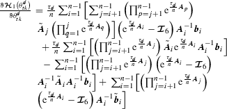
• $\frac{\partial \varvec{\mathcal J}_{1}\left( \theta ^{d}_{tk}\right) }{\partial \theta ^{d}_{tk}} = \frac{\tau _{d}}{n}\sum _{i=1}^{n-1}\left( \prod _{j=i+1}^{n-1} \mathrm{e}^{\frac{\tau _{d}}{n}\varvec{A}_{j}}\right) \tilde{\varvec{A}}_{i}\mathrm{X}$ $\left( \prod _{l=1}^{i}\mathrm{e}^{\frac{\tau _{d}}{n}\varvec{A}_{l}}\right)$,

• $\frac{\partial \varvec{\mathcal J}_{2}\left( \hat{\tau }_{k},\theta ^{d}_{tk}\right) }{\partial \theta ^{d}_{tk}} = \hat{\tau }_{k}\tilde{\varvec{A}}_{n}\varvec{\mathcal J}_{2}\left( \hat{\tau }_{k},\theta ^{d}_{tk}\right)$,

• ,

• $\frac{\partial \varvec{\mathcal H}_{2}\left( \hat{\tau }_{k}, \theta ^{d}_{tk}\right) }{\partial \theta ^{d}_{tk}} = \frac{\partial \varvec{\mathcal J}_{2}\left( \hat{\tau }_{k}, \theta ^{d}_{tk}\right) }{\partial \theta ^{d}_{tk}}\varvec{A}_{n}^{-1}\varvec{b}_{n} - \left( \varvec{\mathcal J}_{2}\left( \hat{\tau }_{k},\theta ^{d}_{tk}\right) \right. \left. - \varvec{\mathcal I}_{6}\right) \varvec{A}_{n}^{-1}\left( \tilde{\varvec{A}}_{n} \varvec{A}_{n}^{-1}\varvec{b}_{n} + \tilde{\varvec{b}}_{n}\right)$.

Appendix 4

In this appendix, we demonstrate that $\frac{\partial {\mathcal L}_{1}\left( \varvec{\mathcal {P}}\left( \varvec{x}_{k}^{-}, \hat{\tau }_{k}, \theta ^{d}_{tk}\right) \right) }{\partial \hat{\tau }_{k}}$ $={\mathcal L}_{2}\left( \varvec{\mathcal {P}}\left( \varvec{x}_{k}^{-}, \hat{\tau }_{k}, \theta ^{d}_{tk}\right) \right)$.

First, the derivative of the function ${\mathcal L}_{1}\Big (\varvec{\mathcal {P}}\Big (\varvec{x}_{k}^{-}, \hat{\tau }_{k}, \theta ^{d}_{tk}\Big )\Big )$ with respect to $\hat{\tau }_{k}$ yields:

$$\begin{aligned}&\frac{\partial {\mathcal L}_{1} \left( \varvec{\mathcal {P}}\left( \varvec{x}_{k}^{-}, \hat{\tau }_{k}, \theta ^{d}_{tk}\right) \right) }{\partial \hat{\tau }_{k}}\nonumber \\&\quad = \frac{\partial {\mathcal L}_{1}\left( \varvec{\mathcal {P}}\left( \varvec{x}_{k}^{-}, \hat{\tau }_{k}, \theta ^{d}_{tk}\right) \right) }{\partial \varvec{\mathcal {P}}\left( \varvec{x}_{k}^{-}, \hat{\tau }_{k}, \theta ^{d}_{tk}\right) }\frac{\partial \varvec{\mathcal {P}}\left( \varvec{x}_{k}^{-}, \hat{\tau }_{k}, \theta ^{d}_{tk}\right) }{\partial \hat{\tau }_{k}}. \end{aligned}$$

(56)

Furthermore, according to “Appendix 3”, and as $\varvec{A}_{n}\varvec{\mathcal J}_{2}\left( \hat{\tau }_{k},\theta ^{d}_{tk}\right) = \varvec{\mathcal J}_{2}\left( \hat{\tau }_{k},\theta ^{d}_{tk}\right) \varvec{A}_{n}$, and taking into account that $\varvec{\mathcal G}_{1}\left( \varvec{x}_{k}^{-}, \theta ^{d}_{tk}\right) \! {=} \varvec{\mathcal J}_{1}\left( \theta ^{d}_{tk}\right) \varvec{h}\left( \varvec{x}_{k}^{-}\right) {+} \varvec{\mathcal H}_{1}\left( \theta ^{d}_{tk}\right)$, it follows that:

$$\begin{aligned}&\frac{\partial \varvec{\mathcal P}\left( \varvec{x}_{k}^{-}, \hat{\tau }_{k}, \theta ^{d}_{tk}\right) }{\partial \hat{\tau }_{k}}\nonumber \\&\quad = \varvec{\mathcal J}_{2}\left( \hat{\tau }_{k}, \theta ^{d}_{tk}\right) \left[ \varvec{A}_{n}\varvec{\mathcal G}_{1}\left( \varvec{x}_{k}^{-}, \theta ^{d}_{tk}\right) + \varvec{b}_{n}\right] , \end{aligned}$$

(57)

In addition, multiplying the first expression of the constrained controlled Poincaré map in (33) by the matrix $\varvec{A}_{n}$, and as $\varvec{A}_{n}\varvec{\mathcal H}_{2}\left( \hat{\tau }_{k},\theta ^{d}_{tk}\right) = \left( \varvec{\mathcal J}_{2}\left( \hat{\tau }_{k},\theta ^{d}_{tk}\right) -\varvec{I}_{6}\right) \varvec{b}_{n}$, we can prove that:

$$\begin{aligned}&\!\!\!\varvec{A}_{n}\varvec{\mathcal {P}}\left( \varvec{x}_{k}^{-}, \hat{\tau }_{k}, \theta ^{d}_{tk}\right) + \varvec{b}_{n}\nonumber \\&\!\!\!\quad = \varvec{\mathcal J}_{2}\left( \hat{\tau }_{k},\theta ^{d}_{tk} \right) \left[ \varvec{A}_{n} \varvec{\mathcal G}_{1} \left( \varvec{x}_{k}^{-}, \theta ^{d}_{tk}\right) + \varvec{b}_{n}\right] . \end{aligned}$$

(58)

Hence, according to (57) and (58), we deduce that:

$$\begin{aligned} \frac{\partial \varvec{\mathcal P}\left( \varvec{x}_{k}^{-}, \hat{\tau }_{k}, \theta ^{d}_{tk}\right) }{\partial \hat{\tau }_{k}} = \varvec{A}_{n}\varvec{\mathcal {P}}\left( \varvec{x}_{k}^{-}, \hat{\tau }_{k}, \theta ^{d}_{tk}\right) + \varvec{b}_{n}. \end{aligned}$$

(59)

Since $\varvec{x}_{k+1}^{-} = \varvec{\mathcal {P}}\left( \varvec{x}_{k}^{-}, \hat{\tau }_{k}, \theta ^{d}_{tk}\right)$, then we obtain:

$$\begin{aligned} \frac{\partial \varvec{\mathcal P}\left( \varvec{x}_{k}^{-}, \hat{\tau }_{k}, \theta ^{d}_{tk}\right) }{\partial \hat{\tau }_{k}} = \varvec{A}_{n}\varvec{x}_{k+1}^{-} + \varvec{b}_{n}. \end{aligned}$$

(60)

As a result, it states that:

$$\begin{aligned} \frac{\partial \varvec{\mathcal P}\left( \varvec{x}_{k}^{-}, \hat{\tau }_{k}, \theta ^{d}_{tk}\right) }{\partial \hat{\tau }_{k}} = \dot{\varvec{x}}_{k+1}^{-}. \end{aligned}$$

(61)

Hence, expression (56) is equivalent to:

$$\begin{aligned} \frac{\partial {\mathcal L}_{1}\left( \varvec{\mathcal {P}}\left( \varvec{x}_{k}^{-}, \hat{\tau }_{k}, \theta ^{d}_{tk}\right) \right) }{\partial \hat{\tau }_{k}} = \frac{\partial {\mathcal L}_{1}\left( \varvec{x}_{k+1}^{-}\right) }{\partial \varvec{x}_{k+1}^{-}}\dot{\varvec{x}}_{k+1}^{-}. \end{aligned}$$

(62)

In fact, relying on (10), we have ${\mathcal L}_{2}\left( \varvec{x}\right) = \frac{\partial {\mathcal L}_{1}\left( \varvec{x}\right) }{\partial \varvec{x}}\dot{\varvec{x}}$, then ${\mathcal L}_{2}\left( \varvec{x}_{k+1}^{-}\right) = \frac{\partial {\mathcal L}_{1}\left( \varvec{x}_{k+1}^{-}\right) }{\partial \varvec{x}_{k+1}^{-}}\dot{\varvec{x}}_{k+1}^{-}$. Hence, expression (62) is reformulated as follows:

$$\begin{aligned} \frac{\partial {\mathcal L}_{1}\left( \varvec{\mathcal {P}}\left( \varvec{x}_{k}^{-}, \hat{\tau }_{k}, \theta ^{d}_{tk}\right) \right) }{\partial \hat{\tau }_{k}} = {\mathcal L}_{2}\left( \varvec{\mathcal {P}}\left( \varvec{x}_{k}^{-}, \hat{\tau }_{k}, \theta ^{d}_{tk}\right) \right) . \end{aligned}$$

(63)

Finally, we stress that:

$$\begin{aligned} {\mathcal L}_{2}\left( \varvec{\mathcal {P}}\left( \varvec{x}_{k}^{-}, \hat{\tau }_{k}, \theta ^{d}_{tk}\right) \right) <0. \end{aligned}$$

(64)

Appendix 5

To achieve stabilization of the linearized controlled Poincaré map (34) by means of the control law (35), we define the following classical candidate Lyapunov function [34]:

$$\begin{aligned} V\left( \varDelta \varvec{x}_{k}^{-}\right) = {\varDelta \varvec{x}_{k}^{-}}^{T}\varvec{\mathcal S}\varDelta \varvec{x}_{k}^{-}, \end{aligned}$$

(65)

with $\varvec{\mathcal S}$ is a positive definite symmetric matrix.

Hence, the research for the matrix gain $\varvec{\mathcal K}$ lies in solving the following linear matrix inequality (LMI):

$$\begin{aligned} \left[ \begin{array}{cc} \varvec{\mathcal S} &{} {\mathcal D}\varvec{\mathcal P}_{\varvec{x}_{k}^{-}}^{*}\varvec{\mathcal S} + {\mathcal D}\varvec{\mathcal P}_{\theta ^{d}_{tk}}^{*} \varvec{\mathcal R} \\ \left( {\mathcal D}\varvec{\mathcal P}_{\varvec{x}_{k}^{-}}^{*}\varvec{\mathcal S} + {\mathcal D}\varvec{\mathcal P}_{\theta ^{d}_{tk}}^{*} \varvec{\mathcal R}\right) ^{T} &{} \varvec{\mathcal S} \end{array} \right] >0,\nonumber \\ \end{aligned}$$

(66)

with ${\mathcal D}\varvec{\mathcal P}_{\varvec{x}_{k}^{-}}^{*} = {\mathcal D}\varvec{\mathcal P}_{\varvec{x}_{k}^{-}}\left( \varvec{x}_{*}^{-}, \hat{\tau }_{*}, \theta ^{d}_{t*}\right) , {\mathcal D}\varvec{\mathcal P}_{\theta ^{d}_{tk}}^{*} = {\mathcal D}\varvec{\mathcal P}_{\theta ^{d}_{tk}}$ $\left( \varvec{x}_{*}^{-}, \hat{\tau }_{*}, \theta ^{d}_{t*}\right)$, and $\varvec{\mathcal R}=\varvec{\mathcal K}\varvec{\mathcal S}$.

In this LMI, the two unknown matrices are $\varvec{\mathcal S}$ and $\varvec{\mathcal R}$. The gain $\varvec{\mathcal K}$ of the control law (35) is then expressed by:

$$\begin{aligned} \varvec{\mathcal K} = \varvec{\mathcal R}\varvec{\mathcal S}^{-1}. \end{aligned}$$

(67)

References

McGeer, T.: Passive dynamic walking. Int. J. Robot. Res. 9(2), 62–68 (1990)
Goswami, A., Thuilot, B., Espiau, B.: A study of the passive gait of a compass-like biped robot: symmetry and chaos. Int. J. Robot. Res. 17, 1282–1301 (1998)
Garcia, M., Chatterjee, A., Ruina, A., Coleman, M.: The simplest walking model: stability, complexity, and scaling. ASME J. Biomech. Eng. 120, 281–288 (1998)
Wisse, M., Schwab, A.L., Van Der Helm, F.C.T.: Passive dynamic walking model with upper body. Robotica 22, 681–688 (2004)
Safa, A.T., Saadat, M.G., Naraghi, M.: Passive dynamic of the simplest walking model: replacing ramps with stairs. Mech. Mach. Theory 42(10), 1314–1325 (2007)
Rushdi, K., Koop, D., Wu, C.Q.: Experimental studies on passive dynamic bipedal walking. Robot. Auton. Syst. 62(4), 446–455 (2014)
Iqbal, S., Zang, X.Z., Zhu, Y.H., Zhao, J.: Bifurcations and chaos in passive dynamic walking: a review. Robot. Auton. Syst. 62(6), 889–909 (2014)
Asano, F.: Efficiency analysis of 2-period dynamic bipedal gaits. In: Proceedings of the IEEE/RSJ International Conference on Intelligent Robots and Systems, pp. 173–180. St. Louis, USA (2009)
Chyou, T., Liddell, G.F., Paulin, M.G.: An upper-body can improve the stability and efficiency of passive dynamic walking. J. Theor. Biol. 285, 126–135 (2011)
Iida, F., Tedrake, R.: Minimalistic control of biped walking in rough terrain. Auton. Robots 28(3), 355–368 (2010)
Gritli, H., Khraeif, N., Belghith, S.: A period-three passive gait tracking control for bipedal walking of a compass-gait biped robot. In: Proceedings of the International Conference on Communications, Computing and Control Applications, pp. 1–6. Hammamet, Tunisia (2011)
Spong, M.W., Bullo, F.: Controlled symmetries and passive walking. IEEE Trans. Autom. Control 50, 1025–1031 (2005)
Spong, M.W., Holm, J.K., Dongjun, L.: Passivity-based control of bipedal locomotion. IEEE Robot. Autom. Mag. 14(2), 30–40 (2007)
Gritli, H., Khraeif, N., Belghith, S.: Semi-passive control of a torso-driven compass-gait biped robot: bifurcation and chaos. In: Proceedings of the International Multi-conference on Systems, Signals and Devices, pp. 01–06. Sousse, Tunisia (2011)
Gritli, H., Belghith, S., Khraeif, N.: Intermittency and interior crisis as route to chaos in dynamic walking of two biped robots. Int. J. Bifurc. Chaos 22(3), Paper no. 1250056 (2012)
Gritli, H., Belghith, S., Khraeif, N.: Cyclic fold bifurcation and boundary crisis in dynamic walking of biped robots. Int. J. Bifurc. Chaos 22(10), Paper no. 1250257 (2012)
Chevallereau, C., Bessonnet, G., Abba, G., Aoustin, Y.: Bipedal Robots: Modeling, Design and Walking Synthesis Wiley-ISTE, 1st edn. Wiley, London (2009)
Li, Q., Yang, X.S.: New walking dynamics in the simplest passive bipedal walking model. Appl. Math. Model. 36(11), 5262–5271 (2012)
Li, Q., Tang, S., Yang, X.S.: New bifurcations in the simplest passive walking model. Chaos Interdiscip. J. Nonlinear Sci. 23, 043110 (2013)
Gritli, H., Khraeif, N., Belghith, S.: Cyclic-fold bifurcation in passive bipedal walking of a compass-gait biped robot with leg length discrepancy. In: Proceedings of the IEEE International Conference on Mechatronics, pp. 851–856. Istanbul, Turkey (2011)
Gritli, H., Khraeif, N., Belghith, S.: Period-three route to chaos induced by a cyclic-fold bifurcation in passive dynamic walking of a compass-gait biped robot. Commun. Nonlinear Sci. Numer. Simul. 17(11), 4356–4372 (2012)
Ott, E., Grebogi, C., Yorke, J.A.: Controlling chaos. Phys. Rev. Lett. 64(11), 1196–1199 (1990)
Kapitaniak, T.: Controlling Chaos: Theoretical and Practical Methods in Non-linear Dynamics. Academic Press, New York (1996)
Andrievskii, B.R., Fradkov, A.L.: Control of chaos: methods and applications. I. Methods. Autom. Remote Control 64(5), 673–713 (2003)
Andrievskii, B.R., Fradkov, A.L.: Control of chaos: methods and applications. II. Applications. Autom. Remote Control 65(4), 505–533 (2004)
Fradkov, A.L., Evans, R.J.: Control of chaos: methods and applications in engineering. Annu. Rev. Control 29(1), 33–56 (2005)
Fradkov, A.L., Evans, R.J., Andrievsky, B.R.: Control of chaos: methods and applications in mechanics. Philos. Trans. R. Soc. A 364(1846), 2279–2307 (2006)
Suzuki, S., Furuta, K.: Enhancement of stabilization for passive walking by chaos control approach. In: Proceedings of the 15th Triennial World Congress of the IFAC, pp. 133–138. Barcelona, Spain (2002)
Osuka, K., Sugimoto, Y.: Stabilization of quasi-passive-dynamic-walking based on delayed feedback control. In: Proceedings of International Conference on Control, Automation, Robotics and Vision, pp. 803–808. Singapore (2002)
Sugimoto, Y., Osuka, K.: Walking control of quasi passive dynamic walking robot ’Quartet III’ based on continuous delayed feedback control. In: Proceedings of the IEEE International Conference on Robotics and Biomimetics, pp. 606–611. Shenyang, China (2004)
Harata, Y., Asano, F., Taji, K., Uno, Y.: Efficient parametric excitation walking with delayed feedback control. Nonlinear Dyn. 67, 1327–1335 (2012)
Kurz, M.J., Stergiou, N.: An artificial neural network that utilizes hip joint actuations to control bifurcations and chaos in a passive dynamic bipedal walking model. Biol. Cybern. 93, 213–221 (2005)
Kurz, M.J., Stergiou, N.: Hip actuations can be used to control bifurcations and chaos in a passive dynamic walking model. J. Biomech. Eng. 129(2), 216–222 (2007)
Gritli, H., Khraeif, N., Belghith, S.: Chaos control in passive walking dynamics of a compass-gait model. Commun. Nonlinear Sci. Numer. Simul. 18(8), 2048–2065 (2013)
Parker, T.S., Chua, L.O.: Practical Numerical Algorithms for Chaotic Systems. Springer, New York (1989)
Hiskens, I.A., Pai, M.A.: Trajectory sensitivity analysis of hybrid systems. IEEE Trans. Circuits Syst. I 47(2), 204–220 (2000)
Author information
Authors and Affiliations
Corresponding author