An objective and efficient method for estimating probabilistic coastal inundation hazards

Abstract

The joint probability method (JPM) is the traditional way to determine the base flood elevation due to storm surge, and it usually requires simulation of storm surge response from tens of thousands of synthetic storms. The simulated storm surge is combined with probabilistic storm rates to create flood maps with various return periods. However, the map production requires enormous computational cost if state-of-the-art hydrodynamic models with high-resolution numerical grids are used; hence, optimal sampling (JPM-OS) with a small number of (~ 100–200) optimal (representative) storms is preferred. This paper presents a significantly improved JPM-OS, where a small number of optimal storms are objectively selected, and simulated storm surge responses of tens of thousands of storms are accurately interpolated from those for the optimal storms using a highly efficient kriging surrogate model. This study focuses on Southwest Florida and considers ~ 150 optimal storms that are selected based on simulations using either the low fidelity (with low resolution and simple physics) SLOSH model or the high fidelity (with high resolution and comprehensive physics) CH3D model. Surge responses to the optimal storms are simulated using both SLOSH and CH3D, and the flood elevations are calculated using JPM-OS with highly efficient kriging interpolations. For verification, the probabilistic inundation maps are compared to those obtained by the traditional JPM and variations of JPM-OS that employ different interpolation schemes, and computed probabilistic water levels are compared to those calculated by historical storm methods. The inundation maps obtained with the JPM-OS differ less than 10% from those obtained with JPM for 20,625 storms, with only 4% of the computational time.

1 Introduction

Coastal regions throughout much of the world are facing increasing flooding risk due to accelerating sea level rise (e.g., Sweet et al. 2017) and more intense storms with lower central pressure (e.g., Knutson et al. 2010; Emanuel 2013). To enable coastal communities to develop adaptation, mitigation, and resilience strategies, it is essential to develop probabilistic coastal inundation vulnerability maps of coastal regions (e.g., Condon and Sheng 2012). Probabilistic coastal inundation maps can be used to (1) determine property at risk evaluated in monetary units without mitigation alternatives; (2) identify areas of high flood vulnerability for development of mitigation alternatives; (3) determine flood vulnerability of coastal communities and infrastructures; and (4) guide the development of adaptation plan such as the use of green infrastructure to increase flood resilience. While FEMA (2014) has developed probabilistic coastal inundation maps using the traditional joint probability method (JPM, see, e.g., Myers 1970) and the joint probability method with optimal sampling (JPM-OS) (see, e.g., Toro et al. 2010a), their maps do not include the effect of the sea level rise (SLR) and more intense storms in the twenty-first century. Condon and Sheng (2012), on the other hand, developed an improved JPM-OS and used it to determine the coastal inundation maps due to SLR and more intense storms in the twenty-first century. This study further improves the JPM-OS and applies it to develop probabilistic coastal inundation maps in Southwest Florida, where the vulnerability to tropical cyclones and SLR and the population growth ranks among the highest in the USA (Blake et al. 2011; U.S. Census Bureau 2018).

The joint probability method (JPM), developed by Myers (1970) for storm surge studies, is a traditional way to determine the base flood elevation (BFE), which is defined as the 1% annual chance (or 100-year) flood elevation (FEMA 2007). In its contemporary version, JPM attempts to all possible combinations of storm landfall characteristics such as central pressure ($P_{\text{c}}$), radius to maximum wind ($R_{\text{m}}$), storm forward speed ($V_{\text{f}}$), storm heading direction ($\theta$), and the landfall location ($L_{0}$), to define a large set of (~ 10,000–100,000 in principle, but much less in practice in order to reduce computational effort) synthetic storms. These synthetic storms are used by a numerical storm surge model to simulate the storm surge, and the annual exceedance probability is then calculated by using the probabilistic descriptions of storm characteristics and storm rate. JPM is by far the most promising method to estimate the annual exceedance probabilities of storm surge and gives more reliable estimates than other methods (distribution-fitting methods, empirical simulation techniques and Monte Carlo simulation) as shown by Agbley and Basco (2008). It was the primary method adopted by FEMA (2007) to evaluate the storm surge return frequencies. However, the major weakness of JPM is the necessity to simulate a large number of (10,000-100,000) storms, which requires enormous computational time and cost when a high fidelity surge model is used (Toro et al. 2010a; Condon and Sheng 2012).

Recently the joint probability method with optimal sampling (JPM-OS) was developed using different optimization schemes (e.g., Resio 2007; Resio et al. 2008; Toro et al. 2010b; Condon and Sheng 2012; Nadal-Caraballo et al. 2015a). Instead of simulating tens to hundreds of thousands of synthetic storms in JPM, JPM-OS applies interpolation and optimization to a small number (~ 100–200) of optimal storm simulations to retain the accuracy of the BFE. While the JPM-OS methods with various optimization and interpolation schemes all appeared to produce reasonably accurate probabilistic inundation maps with improved efficiency compared to the JPM-based maps, they all have their strengths and weaknesses, as will be shown in Sect. 2.

Several fundamental scientific research questions concerning the JPM-OS remain to be answered before it can be readily applied to a variety of coastal flood studies with ease and confidence. For example: “Is the JPM-OS process for selecting optimal storms objective and independent of the study site?” “Are optimal storms determined by low fidelity surge models (with simpler physics and low grid resolution) comparable to those determined by high fidelity surge models?” “What is the accuracy of the high-resolution probabilistic coastal inundation maps produced by JPM-OS versus the JPM-based maps?” In order to answer these questions, it is necessary to use a highly accurate and efficient JPM-OS method along with an efficient high fidelity surge model which can be used to produce highly accurate probabilistic coastal inundation maps. To measure the accuracy of these maps, the high fidelity model must be so efficient that it can be used to produce the inundation maps using JPM with tens of thousands of storms, and to create a benchmark, against which the optimal sampling and interpolation scheme can be compared. Findings of this study should benefit the research community as well as anyone who uses JPM-OS for coastal flood mapping.

This paper aims to answer the above research questions by using a synthetic storm dataset (which corresponds the period of 1982–2009, see Sect. 4), rather than historical storms that are utilized and analyzed in Condon and Sheng (2012), and two numerical hydrodynamic models to produce probabilistic coastal inundation maps in Southwest Florida (Fig. 1). The objectives of the paper are to improve the methods for selecting optimal storms and interpolating inundation results of optimal storms, as well as to validate the JPM-OS by comparing inundation maps obtained with the JPM, using both a high fidelity model and a low fidelity model. For simplicity, this study focuses on the effects of storm surge and waves. The results should be applicable to other storm data sets (e.g., storm ensemble for 2060 or 2100), other high fidelity models (e.g., ADCIRC and FVCOM), as well as other model domains (e.g., Southeast Florida, Florida Panhandle, and New Jersey and New York coasts). Improved probabilistic coastal inundation maps should enable improved adaptation and mitigation strategies. Effects of future more intense storms, sea level rise, and precipitation will be addressed in a future paper.

Fig. 1

CH3D (left) and SLOSH (right) domains of Southwest Florida

A relatively low fidelity (low resolution and simple physics) and computationally efficient numerical model SLOSH (Jelesnianski et al. 1992) is used to evaluate the responses of all possible synthetic storms in JPM, based on which optimal storms are determined. The optimal storms are then simulated using high fidelity CH3D-SSMS (Sheng et al. 2010a); a state-of-the-art numerical surge model with grid size > 20 m (vs. > 1000 m for SLOSH) and probabilistic coastal inundation maps with various return periods are computed using JPM-OS interpolation process. Moreover, high-resolution probabilistic coastal inundation maps are also produced using CH3D-SSMS and JPM to provide the benchmark. One advantage of using modeled climatology is we can compare the predicted probabilistic water levels with those computed from the measured tidal gauge data (as shown in Sect. 4.8). Moreover, the JPM-OS with kriging interpolation and optimal storm selection introduced in this paper do not depend on the type of storm data used.

This paper adopts a kriging surrogate model as the interpolation scheme of JPM-OS, while the optimization scheme, which uses the Gaussian quadrature to interpolate the surge response of any storm, could be regarded as a hybrid of JPM-OS-RS (Resio 2007) and JPM-OS-Q (Toro et al. 2010a, b). Jia et al. (2016) used the kriging surrogate model with principal component analysis (PCA) to produce good (with R² close to 95% or better and RMSE less than 10%) peak surge response in coastal regions at 30 locations along Louisiana coast, but did not produce any probabilistic coastal inundation map. Zhang et al. (2018) used kriging surrogate model with the database from North Atlantic Comprehensive Coastal Study (NACCS) (Nadal-Caraballo et al. 2015a) to discover the annual exceedance rate with and without SLR. However, their results only focus on two representative locations (Battery, NY and Virginia Beach, VA) but not a large domain. As explained later, the kriging surrogate model does not require tuning because model coefficients are directly calculated by the kriging algorithm; hence, it is objective and allows full automation. The method is so efficient that it takes much less time to generate coastal inundation maps with much improved accuracy, compared to Condon and Sheng (2012).

In the following, the JPM and JPM-OS with kriging are first briefly reviewed, although JPM-OS with variations of the interpolation scheme will also be discussed. Thereafter, the SLOSH and CH3D storm surge models are described briefly, followed by a discussion of the characteristics of the storms for Southwest Florida, which is the focus of this study. Selection process for the optimal storms is then presented. Probabilistic coastal inundation maps obtained using SLOSH and JPM and JPM-OS are then presented, followed by a presentation of probabilistic coastal inundation maps obtained using CH3D and JPM and JPM-OS. Tides in the microtidal SW Florida are relatively low compared to those in the mid-Atlantic coast. They have limited contribution to probabilistic flood elevations as tides have a similar chance to increase or decrease the inundation values. Therefore, tidal effect on probabilistic coastal inundation is less compared to the effects of storm surges and waves. This paper focuses on the processes for the selection of optimal storms and the interpolation of simulated inundation results for the optimal storms, rather than the inclusion of all physical processes for coastal inundation. Precipitation, which is becoming more important in recent hurricanes, is not included in this study for simplicity, but will be addressed in a later study.

For clarity, the annual exceedance probabilities of 2%, 1%, and 0.2% are referred as the 50-year, 100-year and 500-year recurrence level, respectively, which are also called 50-year, 100-year and 500-year return periods by FEMA. It is important to point out that surge level with 50-year return period does not mean that surge level will occur only once every 50 years, but the expected recurrence interval of that surge height is 50 years with an annual chance occurrence of 2%.

2 JPM and JPM-OS

2.1 JPM

The JPM uses the probabilistic descriptions of landfall parameters and storm rate to determine a set of synthetic storms, which are called test storms. A single storm with a set of the five landfall parameters is called a “node ($\varvec{x}$)” in a five-dimensional parameter space:

$$\begin{array}{*{20}c} {x = \left[ {\begin{array}{*{20}l} {P_{\text{c}} } \hfill & {R_{\text{m}} } \hfill & \theta \hfill & {V_{\text{f}} } \hfill & {L_{0} } \hfill \\ \end{array} } \right]} \\ \end{array}$$

(1)

The storms are simulated with a numerical model to generate the peak water level height $\eta (x)$ for the model domain. The annual rate of occurrence of the water level height greater than a specific value $\eta$ for a cell inside the model domain is calculated by the JPM integral (Niedoroda et al. 2010):

$$\begin{array}{*{20}c} {P\left[ {\eta_{ \hbox{max} } > \eta } \right] = \lambda \mathop \int \nolimits \ldots \mathop \int \limits_{\varvec{x}}^{ } f_{\varvec{X}} \left( \varvec{x} \right)P\left[ {\eta \left( \varvec{x} \right) > \eta } \right]{\text{d}}\varvec{x}} \\ \end{array}$$

(2)

The integral depends on the mean annual rate $\lambda$ of all storms for the domain, the joint probability density function $f_{\varvec{X}} (\varvec{x})$, and the conditional probability (Heaviside function) that a certain set of storm characteristics $\varvec{x}_{i}$ will generate a water level height greater than $\eta$, is $P[\eta (\varvec{x}_{i} ) > \eta ]$. The integral is evaluated for all test storms, and the annual probability, which has the unit of storms per unit time, is calculated.

The joint probability density function as shown in Eq. (2) is difficult to calculate. Instead, the annual probability for the storms to produce water level exceeding a certain value $\eta$ can be approximately calculated by using the following formula as

$$\begin{array}{*{20}c} {P\left[ {\eta_{ \hbox{max} } > \eta } \right] \approx \mathop \sum \limits_{i = 1}^{n} \lambda_{i} P[\eta (\varvec{x}_{i} ) > \eta ]} \\ \end{array}$$

(3)

where $n$ is the number of the test storms, and $P$ is the probability of the storm with the landfall characteristics $\varvec{x}_{i}$.

2.2 JPM-OS

In JPM-OS, a small number (usually a few hundred) of storms called “optimal” (representative) storms are selected from the test storms in JPM. The optimal storms are then simulated by using a numerical hydrodynamic model to get the corresponding peak water levels. The peak water levels for all test storms are interpolated from the peak water levels of optimal storms, and the flood maps are calculated as discussed in Sect. 2.1.

Variations of the JPM-OS use different optimization interpolation schemes: RS (response surface), BQ (Bayesian quadrature), SRF (surge response function), and MARS (multivariate adaptive regression splines). Detailed discussion on the development of these JPM-OS methods is given by Toro et al. (2010a, b) (JPM-OS-Q and JPM-OS-RS), Condon and Sheng (2012) (JPM-OS-MARS) and Resio et al. (2017) (JPM-OS-BQ and JPM-OS-SRF). Resio et al. (2017) presented a comprehensive review of the methods (historical storm method, JPM, empirical simulation technique, stochastic-deterministic track method, JPM-OS-BQ, and JPM-OS-SRF) to quantify coastal storm surge, and discussed the aleatory and epistemic uncertainties of JPM and JPM-OS.

Although the various JPM-OS methods are all robust methods, they could be further improved. For example, for determining the optimal storms for JPM-OS-BQ and JPM-OS-RS and the correlation distance for JPM-OS-BQ, sensitivity tests and expert judgement are required, which make the methods less objective and incapable of automation. The number of parameters considered by JPM-OS-SRF is limited, which does not allow the inclusion of more variables such as tide and sea level rise in the formulation. The JPM-OS-MARS requires defining spline coefficients, which are domain-specific. The optimization schemes of JPM-OS-RS, JPM-OS-BQ and JPM-OS-SRF were applied only to tens or hundreds of coastal stations, while the optimization scheme of JPM-OS-MARS was applied to hundreds of thousands of coastal and inland stations.

2.3 JPM-OS with kriging

A kriging model is a Gaussian process surrogate model that assumes the value at a point is correlated to the values at neighboring points and is weighted according to spatial covariance values. It is also known as the best linear unbiased predictor (Sacks et al. 1989). In this study, the MATLAB toolbox “DACE” (Lophaven et al. 2002) is used for kriging interpolation with parallelism. The details are described below.

Suppose there are $m$ optimal storms $\varvec{X}$ = $\left[ {\varvec{x}_{1} \ldots \varvec{x}_{m} } \right]^{\text{T}}$ with $\varvec{x}_{i} \in {\mathbb{R}}^{p}$ ($p = 5$ in this study) and the corresponding water levels are $\varvec{Y = }\left[ {\varvec{y}_{1} \ldots \varvec{y}_{m} } \right]^{\text{T}}$ with $\varvec{y}_{i} \in {\mathbb{R}}^{q}$. The water level (rather than inundation height, in order to ensure spatial smoothness) is used in the interpolation to ensure smooth interpolated results. The value of $q$ could be selected from 1 to the number of land cells ($N_{c}$). In practice, $q$ is often selected as 1 or $N_{c}$. If $q$ = 1, every cell inside the domain has a set of kriging coefficients. This method produces more accurate results, but it takes more computing resources. It will be referred to as “accurate kriging”, and the corresponding JPM-OS will be called JPM-OS-AK (JPM-OS with accurate kriging). If $q = N_{\text{c}}$, then all cells inside the domain have the same set of kriging coefficients. The corresponding interpolated flood maps are less accurate, but it takes less time to finish. This method is referred to as “quick kriging”, and the corresponding JPM-OS will be called JPM-OS-QK (JPM-OS with quick kriging). Additional details of kriging calculations are provided in “Appendix”.

3 Modeling systems and study domains

The Sea, Lake, and Overland Surges from Hurricanes (SLOSH) (Jelesnianski et al. 1992) is a 2-D numerical hydrodynamic model used to estimate storm surge heights and produce flood maps by considering the atmospheric pressure, size, forward speed, and track data of the hurricanes (Zachry et al. 2015). It is an efficient numerical model usually running on a coarse grid with grid spacing greater than 1 km. Because of its efficiency (a few minutes CPU time for one forecast cycle), it is used in this study for the determination of optimal storms in JPM-OS. Although SLOSH does not consider wave effects and surge-tide interactions, the model is accurate to within ± 20% of observed water level according to NOAA (2013).

Curvilinear-grid hydrodynamics in 3D (CH3D) is a hydrodynamic model, originally developed by Sheng (1987, 1990) which can simulate 2-D and 3-D barotropic and baroclinic circulation driven by tide, wind and density gradients. A boundary-fitted non-orthogonal curvilinear grid is used in the horizontal direction, and terrain-following sigma grid is used in the vertical direction in CH3D, to enable accurate resolution of the complex shorelines and geometries in coastal regions. The numerical model satisfies conservation for momentum, water mass, water temperature and salinity, by using finite-volume method of formulation. A Smagorinsky-type model for horizontal turbulent mixing and a turbulent-kinetic-energy (TKE) turbulence closure model for vertical turbulent mixing (Sheng and Villaret 1989) are used in CH3D. Due to the use of a semi-implicit numerical algorithm, CH3D is much more efficient than many other high fidelity hydrodynamic models [e.g., ADCIRC (Luettich et al. 1992), POM (Peng et al. 2004), FVCOM (Weisberg and Zheng 2006)] when similar high-resolution grid is used (Sheng et al. 2012a). Therefore, in this study, CH3D is dynamically coupled to SWAN (Booij et al. 1999) to simulate surge, wave, and flooding in high-resolution coastal region, while ADCIRC and WaveWatch-III (Tolman 2009) are used to provide offshore open boundary conditions for CH3D and SWAN, respectively. This integrated storm surge modeling system, CH3D-SSMS (Sheng et al. 2006), is capable of simulating flooding and drying and has been used extensively for simulating and forecasting numerous storm surges along the US Atlantic and Gulf coasts (e.g., Sheng et al. 2010a, b; Davis et al. 2010; Paramygin et al. 2016; Sheng and Zou 2017). In a US Southeastern Regional Storm Surge Model Testbed (Sheng et al. 2012a), it was found that CH3D-SSMS was the most efficient high fidelity surge model, following closely behind the low fidelity SLOSH model, while possessing similar accuracy as other high fidelity models. Details of CH3D and CH3D-SSMS can be found in Sheng et al. (2010a).

In this study, CH3D is used as the state-of-the-art high fidelity numerical model for use with JPM and JPM-OS, driven by a synthetic parametric wind model (Holland 1980). The wind and pressure fields are calculated based on location of the storm, pressure at the center, radius to maximum winds and translational velocity of the storm. An ensemble of storm tracks, which are straight line tracks with all parameters kept constant until landfall and then allowed to decrease, is created following Condon and Sheng (2012). For simplicity, the storms are simulated by running CH3D model in a 2D vertically averaged mode, instead of the 3D mode. Results obtained with the 3D vegetation-resolving CH3D model will be reported in a later paper.

Southwest Florida is selected as the study domain (Fig. 1), of which the CH3D grid has 386,140 cells and a minimum resolution of 20 m in coastal areas with the average grid size of about 200 m. The bottom friction formulation in CH3D model uses a spatially varying Manning’s coefficient, which is determined from the US Geological Survey (USGS Survey 2011) data with a value of 0.02 in the open water. The SLOSH domain “efm2” is shown in Fig. 1, which has 11,100 cells and a minimum resolution of ~ 200 m and the average grid size of ~ 1500 m. CH3D domain has significantly higher spatial resolution, compared to SLOSH. In this study, all elevations are referred to the NAVD88 vertical datum. The inundation elevation is the difference between the water level and the local topography. The bathymetry data are based on GEOphysical DAta System (GEODAS 2009), and the topography data are based on the National Elevation Dataset (USGS NED 2009). The bathymetry and topography as shown in Fig. 1 have very gentle slopes, which make the region prone to coastal inundation by surge and wave.

4 Application to Southwest Florida

4.1 Storm data

The storm data are developed by LaRow et al. (2014) using the FSU—COAPS model (Kozar and Misra 2013) and Liu et al. (2014) using the WRF (Weather Research Forecast) model (Skamarock et al. 2008) for the current climate (1982–2009). A dynamical downscaling technique, the scale selective data assimilation (SSDA) approach, together with statistical downscaling methods are applied to the storm data of LaRow et al. (2014) to project the tropical cyclones (TCs) striking Southeast US coast region (Liu et al. 2014). Storms that make landfall in Florida are plotted in Fig. 2 where CREF represents the simplified shoreline. There are 60 TCs in this region during the simulation period, of which seven TCs made landfall on Southwest Florida. These numbers compare well with the 64 historical storms with seven landfalls during the same time period for the region. The TCs with pressure deficit greater than 20mb at landfall are used in this study.

Fig. 2

Simulated storm tracks (blue lines), simplified coastline (red line), and center of reference (CREF) of Southwest Florida. CREF is located at (27.164N, 82.517W) near Sarasota, FL

4.2 Distributions of landfall parameters

The central pressure deficit, radius to maximum wind, storm forward speed, and storm heading direction of landfalling storms in Southwest Florida are found from the storm data. Exiting storms are not considered. By following the method in Condon and Sheng (2012), best fits of the data to known distribution functions are found using maximum likelihood estimation (Le Cam 1990). The central pressure deficit, radius to maximum wind, and storm forward speed are found to best fit a Weibull distribution (Devroye 1986), and the storm heading directions are found to best fit a Type-1 extreme value distribution (Kotz and Nadarajah 2000). The probability density functions (PDFs) of the distributions are shown in Fig. 3.

Fig. 3

PDFs of hurricane landfall parameters for Southwest Florida. a Central pressure deficit ($P_{\text{c}}$), b radius to maximum wind ($R_{\text{m}}$), c forward speed ($V_{\text{f}}$), and d storm heading ($\theta$)

To calculate the flood maps based on JPM, several representative values have to be selected from the PDFs of the landfall parameters (Toro et al. 2010a). In this study, five values are selected for each of the four parameters: $P_{\text{c}}$, $R_{\text{m}}$, $\theta$, $V_{\text{f}}$, and 33 values for $L_{0}$ (landfall location every 10 nautical miles of the coast). The central pressure deficit is discretized to evenly sized bins, with minimum of 13.5 mb and maximum of 78.5 mb, and bin size of 13 mb. The representative values are selected as median values of the bins. The same method is applied to radius to maximum wind, storm forward speed and storm heading direction. The entire parameter space of each parameter is covered and each parameter is evenly discretized to avoid any bias in storm selection (Condon and Sheng 2012). The ensemble contains a total of 20,625 storms which cover all combinations of discretized parameters. Each combination of parameters is assigned a rate of occurrence. The representative values and corresponding probabilities for the landfall parameters other than landfall locations are shown in Table 1. The distributions of storm parameters in this study are similar to those of historical storms (Condon and Sheng, 2012). Although the radii of maximum wind are somewhat overestimated, it did not lead to significant difference in the resulting inundation map.

Table 1 The representative values of the landfall parameters and corresponding probabilities (in the parenthesis) for traditional JPM

Resio et al. (2017) discussed the correlation between storm heading and central pressure deficit (intensity) and showed that including the correlation would affect the return period of central pressure. However, the low correlation coefficient (0.02) between storm heading and intensity indicates that they are independent in this study. The intensity and radius to maximum wind (RMW) are usually correlated in the way that the more intense storms tend to have smaller radius (see Toro et al. 2010b; Condon and Sheng 2012). However, Vickery and Wadhera (2008) found that for Gulf of Mexico landfalling hurricanes, the landfall values of RMW are not a function of pressure and latitude. The weak correlation coefficient (− 0.15) between the two parameters shows that they could be treated as independent parameters in this study.

4.3 Storm rates

The storm rates are calculated following the method of Chouinard and Liu (1997). The omni-directional storm rate $\lambda$ of 3.1658E − 04 storms/year/km is achieved by taking distance of a storm to the location of interest $L_{\text{o}}$, and by using kernel estimator. The normal distribution function is used as a kernel function, and cross-validation is used to find the optimal degree of smoothness. The calculated omni-directional storm rate has the unit of storms/year/km. Figure 4 shows the storm rate, which is fitted to a seventh-order polynomial as a function of the distance from the CREF.

Fig. 4

Storm rate as a function ($L_{0}$) of distance from CREF, obtained by seventh order polynomial fit

4.4 Selection of optimal storms

To perform kriging interpolation, a number of optimal storms (also referred to as training storms in literature) are selected from the large number of test storms. The optimal storms consist of two parts, fundamental and additional optimal storms. Every combination of parameters can be represented as a point (node) in a 5-D space. These nodes have coordinates equal to the values of discretized parameters and hence 20,625 storms form a grid in a 5-D space where nodes are intersections of planes with one of the coordinates held as constant and equal to a discretized value. The fundamental nodes are selected by Steps 1–3 in the following. While the 5-D case cannot be illustrated, examples of nodes in 2-D and 3-D spaces are shown in Fig. 5.

Fig. 5

2D and 3D examples of steps 1–3 in optimal storm selection. Red, green and yellow nodes represent the selected fundamental storms in step 1, 2 and 3, respectively

• Step 1 Select the outer nodes of the grid formed by the planes, yielding 32 (2⁵) optimal nodes.

• Step 2 Select the center nodes of edges of the grid, yielding 80 (5*2⁴) optimal nodes.

• Step 3 Select the center node of the grid, yielding 1 optimal node.

  If the number of parameters in JPM is n, then the number of fundamental nodes selected in Steps 1–3 is

  $$\begin{array}{*{20}c} {(2^{n} + n*2^{{\left( {n - 1} \right)}} + 1)} \\ \end{array}$$

  (4)

  The red, green and yellow nodes in Fig. 5 illustrate the nodes selected in Steps 1, 2 and 3, respectively. There are 113 fundamental optimal nodes selected. Such selection ensures that the training set covers the realm of possible storms at a location, and no extrapolation is required, since kriging accuracy cannot be guaranteed in the extrapolation zone (Lophaven et al. 2002). This is an important part of these schemes, as it is essential that the training set needs to cover the realm of possible storms at a location. The additional optimal nodes are selected by following Steps 4–5.

• Step 4 Perform simulations of 20,625 test storms from the entire ensemble using the SLOSH model and calculate the corresponding total inundation volumes (TIV) (see Sheng et al. 2012b):

  $$\begin{array}{*{20}c} {TIV = \mathop \sum \limits_{i = 1}^{{N_{\text{c}} }} A_{i} *H_{i} } \\ \end{array}$$

  (5)

  where $N_{\text{c}}$ is the number of land cells of the domain, $A_{i}$ is the area of the land cell, and $H_{i}$ is the inundation height of the cell, which is calculated by subtracting bottom elevation of the cell from the simulated maximum envelope of water (MEOW, maximum water level over a single storm simulation) $\eta_{i}$ of the cell. TIV is used as an objective index to quantify the storm surge over the entire domain caused by a single storm.

• Step 5 Calculate five-dimensional gradients of TIVs for all test nodes:

  $$\begin{array}{*{20}c} {g = \left[ {g_{x1} , g_{x2} , g_{x3} , g_{x4} , g_{x5} } \right]} \\ \end{array}$$

  (6)

  where $g_{x1}$, $g_{x2}$, $g_{x3}$, $g_{x4}$, and $g_{x5}$ are the gradient of TIV with respect to central pressure deficit, radius of maximum wind, storm forward speed, storm heading direction, and landfall location, respectively. The absolute value of $\varvec{g}$ is

  $$\begin{array}{*{20}c} {\left| \varvec{g} \right| = \sqrt[2]{{g_{x1}^{2} + g_{x2}^{2} + g_{x3}^{2} + g_{x4}^{2} + g_{x5}^{2} }}} \\ \end{array}$$

  (7)

  The values of $|\varvec{g}|$ of every test storm are ranked from highest to lowest, and the nodes with largest N_a values of $|\varvec{g}|$ corresponding to those most influential storms are selected as the additional nodes. The number of additional nodes N_a is determined by defining desired accuracy (according to Fig. 6) and available computing resources required to perform model simulations. For this particular study, N_a is chosen to be 37.

  Fig. 6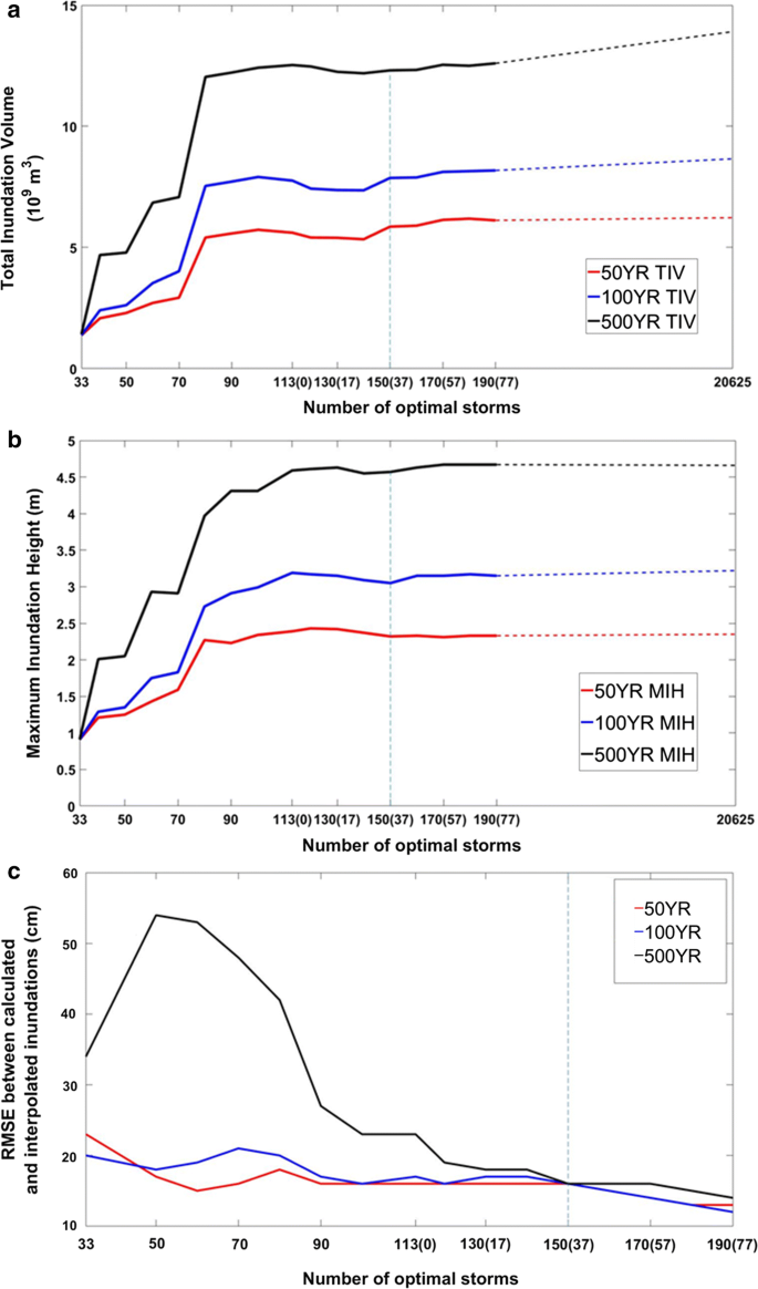

  

  a TIV versus number of optimal storms. b MIH versus number of optimal storms. c RMSE between calculated and interpolated inundations versus number of optimal storms. The number in the parenthesis indicates the number of additional optimal storms selected in step 5. The right end of the dash lines of a and b indicates the TIV and MIH results by JPM using 20,625 test storms

Figure 6 shows the dynamics of TIV, maximum inundation height (MIH; defined as the maximum inundation height within the model domain during the entire storm period), and the root-mean-square error (RMSE) between calculated and interpolated inundation heights of the flood maps with 50-, 100- and 500-year return periods, with the number of optimal storms used in kriging interpolation. The number in the parenthesis indicates the number of additional storms selected in step 5, and no additional nodes are selected if the total number of optimal storms is less than or equal to 113. The number of additional nodes is determined by plotting the curves similar to those shown in Fig. 6 and selecting the desired level of accuracy. The additional nodes are needed to improve the accuracy of interpolation over the storms that have relatively large inundation volumes. These storms are the ones that matter in determining the flood maps with 50-, 100- and 500-year return periods. The workflow of JPM and JPM-OS is shown in Fig. 7.

Fig. 7

JPM and JPM-OS workflow schematic

4.5 Inundation maps obtained using SLOSH with JPM and JPM-OS

To ensure accurate probabilistic coastal inundation maps, it is important to analyze the differences between maps interpolated by JPM-OS and maps produced by JPM. In order to compare the accuracy of interpolation using the JPM-OS, different interpolation methods are tested. All test storms are simulated with SLOSH, and 150 optimal storms are selected as shown in Sect. 4.4. Maximum water levels from the optimal storm ensemble are interpolated onto the test storm ensemble by using kriging interpolation. Then the flood maps with 50-, 100- and 500-year return periods are calculated using JPM, JPM-OS-AK and JPM-OS-QK. The PCA method (referred to as JPM-OS-PCA hereafter) by Jia et al. (2016) was coupled with JPM-OS-QK and tested with the largest 60 eigenvectors. The PCA coupled with JPM-OS-AK will produce similar results. Another interpolation scheme that was tested is JPM-OS-MARS by Condon and Sheng (2012).

Flood maps with 50-, 100- and 500-year return periods using the five methods above are shown in Fig. 8. Statistics of the flood maps produced by JPM, JPM-OS-AK, JPM-OS-QK, JPM-OS-PCA and JPM-OS-MARS, and the computational time needed to calculate model coefficients and perform interpolation for all test storms by different methods (on a computer system with a 4-core Intel Core i7-6700 CPU) are listed in Table 2. Coefficients of determination (R²) and RMSE between simulated and interpolated inundation heights are shown in Fig. 9. With 150 optimal storms, RMSE of 100-year flood map is reduced by 1 cm, and RMSE of 500-year flood map is reduced by 7 cm. The 500-year inundation heights with 150 optimal storms are improved locally though not reflected in TIV, compared to the ones obtained with 113 optimal storms.

Fig. 8

Flood maps with 50-year (first column), 100-year (second column) and 500-year (third column) return periods with SLOSH simulations by traditional JPM (first row), JPM-OS-AK (second row), JPM-OS-QK (third row), JPM-OS-PCA (fourth row), and JPM-OS-MARS (fifth row). Horizontal and vertical axes represent longitude and latitude in degrees, respectively

Table 2 Statistics of the SLOSH-based flood maps in Fig. 8 and the computational time of the four JPM-OS methods

Fig. 9

Comparisons between simulated inundation heights by JPM and interpolated inundation heights by JPM-OS-AK (a), JPM-OS-QK (b), JPM-OS-PCA (c), and JPM-OS-MARS (d). The first, second and third subplots of each figure show the comparisons of inundation heights with 50-, 100- and 500-year return periods, respectively

Both JPM-OS-AK and JPM-OS-QK results deviate less than 10% from the JPM results, while the JPM-OS-AK results have slightly larger R² and smaller RMSE. The flood maps with 100- and 500-year return periods by JPM-OS-PCA are underestimated, with RMSE of 0.36 m and 0.82 m. The RMSE of the flood maps by JPM-OS-MARS is two times larger than that by JPM-OS-AK and JPM-OS-QK. Overall, the flood maps by JPM-OS-AK produce the most accurate results.

JPM-OS-PCA is the fastest one of the four methods. The JPM-OS-AK interpolation produces the most accurate result, but it requires the longest computational time. This interpolation method is used to determine the inundation frequencies of Southwest and Southeast Florida for future climate scenarios (Sheng et al. 2019). Interpolation time required for JPM-OS-QK is significantly smaller than that for JPM-OS-AK, but it is only slightly less accurate. Hence, JPM-OS-QK used in a Rapid Forecasting System to generate the flood map of a single storm within minutes of a storm track is available (Yang et al. 2019).

4.6 Inundation maps obtained using CH3D with JPM and JPM-OS

The interpolated results by JPM-OS-AK based on SLOSH model show that it is possible to use interpolation instead of direct simulations (JPM) with little loss of accuracy. To produce detailed high-resolution flood maps, the 150 optimal storms are simulated by CH3D, which has more robust physics and higher grid resolution than SLOSH. Simulated MEOWs are then used in interpolation with JPM-OS-AK. To verify the assumption that the optimal storms selected based on SLOSH simulations are also suitable for interpolation of high-resolution maps based on CH3D simulations and JPM-OS-AK, all test storms are simulated by the high fidelity CH3D and the flood maps are calculated using JPM.

The flood maps with 50-, 100- and 500-year return periods based on JPM and JPM-OS-AK with CH3D simulations are shown in Fig. 10, and the statistics of the flood maps and the total time and disk space needed are shown in Table 3. Figure 11 shows comparisons between JPM-based and JPM-OS-AK-based inundation heights for CH3D simulations. The two sets are in good agreement with less than 10% differences. Comparisons of flood maps of JPM and JPM-OS-AK maps based on SLOSH and CH3D models (Figs. 8, 10) show that CH3D-based maps have smaller TIA and lower MIH than SLOSH-based ones. The RMSE of the water levels between JPM-OS-AK and JPM is 11–13 cm, which is smaller than the RMSE of 20–30 cm by Irish et al. (2009), and 30–50 cm by Taylor et al. (2015). The JPM-OS-AK with CH3D saves more than 95% of time and 99% disk space, while keeping the accuracy comparable to JPM.

Fig. 10

Flood maps with 50-year (first column), 100-year (second column) and 500-year (third column) return periods with CH3D simulations by JPM (first row), and JPM-OS-AK (second row)

Table 3 Statistics of the CH3D-based flood maps in Fig. 10, and the total time and disk space that JPM and JPM-OS-AK take with CH3D simulations

Fig. 11

Comparisons between simulated inundation heights by JPM and interpolated inundation heights by JPM-OS-AK with CH3D simulations. The first, second and third subplots of the figure shows the comparisons of inundation heights with 50-year, 100-year and 500-year return periods, respectively

4.7 Compare the optimal storms determined by SLOSH and CH3D simulations

To answer the question “Are optimal storms determined by low resolution surge models comparable to those determined by high-resolution surge models?”, the optimal storms are selected from the CH3D simulation of the test storms following the optimal storm selection method in Sect. 4.4. The flood maps with 50-, 100- and 500-year return periods by JPM-OS-AK using the optimal storms determined above are shown in Fig. 12. These flood maps are compared with the flood maps that are interpolated by JPM-OS-AK using the optimal storms determined from SLOSH simulations of the test storms in Fig. 10. The differences of the flood maps, most of which are below 1 ft, are shown in Fig. 12. The small differences indicate that the optimal storms determined by low fidelity surge model and the high fidelity surge model and the corresponding flood maps are comparable. Thus, low fidelity surge model should be used to determine optimal storms, while high fidelity surge model should be used to simulate the surge during optimal storms, and JPM-OS-AK should be used to develop high-resolution probabilistic flood maps by interpolation.

Fig. 12

Flood maps with 50-year (upper left), 100-year (upper middle) and 500-year (upper right) return periods by JPM-OS-AK with the optimal storms determined by CH3D simulations of test storms, and the differences of the flood maps with 50-year (lower left), 100-year (lower middle) and 500-year (lower right) by JPM-OS-AK with the optimal storms determined by CH3D simulations of test storms and determined by SLOSH simulations of test storms

4.8 Historical storm method using observed water level data for probabilistic storm surge

It is interesting to compare the probabilistic storm surge produced by CH3D in this study to that obtained using the historical storm method (HSM) which uses the observed water level data to estimate the return period (see, e.g., Katz et al. 2002; Tebaldi et al. 2012). To this end, the hourly observed water level data from 1983 to 2009 (data from 1982 to 1983 are not available) at NOAA tidal station Naples Pier (shown in Fig. 1) are used. It should be noted that this station is on a pier in open water, so the return period water levels are not inundations (as in all figures) but actual water levels. Two approaches are commonly used: the block maxima method (Katz et al. 2002) and the peak-over-threshold method (POT, Nadal-Caraballo et al. 2015b; Tebaldi et al. 2012). The block maxima method first divides the observation period into non-overlapping periods of equal size, which is set to 1 year in this study, and finds the maximum water level within each year. The water levels are then fitted into a generalized extreme value (GEV) distribution, and the return periods are determined from the distribution. The peak-over-threshold method first detrends the hourly observed water level data, computes the daily maxima of water level and selects a threshold corresponding to the 99^th percentile (after trial and error) of observed water levels. Then the threshold exceedances are fitted to a generalized Pareto distribution (GPD), and the return periods are determined from the distribution. Nadal-Caraballo et al. (2015b) used POT with Monte Carlo life-cycle (POT-MCLC) method, which was repeated 10,000 times to compute the mean return periods and confidence limits. The probability distributions and confidence intervals of extreme water levels calculated using POT-MCLC are promising but not the focuses of this study. Thus, the method is not utilized here. Table 4 shows the comparisons of the water levels with 50-year, 100-year and 500-year return periods calculated by block maxima method, peak-over-threshold method and JPM-OS-AK method based on CH3D simulation. The differences of probabilistic water levels with 50-year and 100-year return periods are less than 9% between JPM-OS-AK and POT, and less than 13% between JPM-OS-AK and block maxima. The large differences of probabilistic water level with 500-year return period among the methods are likely due to the limited data used and parametric extrapolation by HSM, which could result in higher variability in the estimates, compared to JPM (Irish et al. 2011; Resio et al. 2017). Additionally, the differences could be due to the fact that the simulated storms from FSU-COAPS model, rather than the historical storms, are used for JPM and JPM-OS in this study.

Table 4 Water levels with 50-year, 100-year and 500-year return periods calculated by block maxima, POT and JPM-OS-AK

5 Conclusion and discussion

This paper presents an accurate and efficient JPM-OS that uses kriging surrogate model as interpolation scheme and an objective method for optimal storm selection to produce probabilistic coastal flood maps with two storm surge models: SLOSH and CH3D. Focusing on Southwest Florida where the threat of hurricane-induced storm surge and coastal flooding is high, the major findings of this study include:

• 1. The efficient numerical storm surge model SLOSH is used to simulate an entire JPM ensemble that consists of 20,625 test storms. From the test storms, 150 optimal storms, which include 113 fundamental optimal storms and 37 additional optimal storms, are quickly and objectively selected. The selected set of optimal storms compares well to the set obtained using CH3D.

• 2. The probabilistic inundation maps of Southwest Florida obtained by JPM-OS with accurate kriging (JPM-OS-AK) using 150 optimal storms deviate less than 20% from the JPM-based maps using 20,625 test storms. This is true for both SLOSH-based and CH3D-based simulations. The RMSE of the water levels between JPM-OS-AK and JPM as shown in Fig. 9 is under 16 cm (0.525 ft) for both hydrodynamic models. This is the first time that the entire JPM ensemble of test storms is simulated with a state-of-the-art numerical hydrodynamic model.

• 3. The JPM-OS with quick kriging (JPM-OS-QK) is also employed in Southwest Florida. The probabilistic flood maps by JPM-OS-QK are slightly less accurate than those by JPM-OS-AK, but require much less computation. JPM-OS-AK is recommended for producing probabilistic flood maps for current and future climate scenarios, and JPM-OS-QK is recommended for quick forecasting of an approaching storm.

• 4. The JPM-OS-AK can be employed to produce flood maps with little loss of accuracy, while the number of simulations is reduced by 1–2 orders of magnitude and the total computational time needed is reduced by an order of magnitude.

• 5. The probabilistic 50-year and 100-year water levels at Naples tidal station produced by JPM-OS-AK compare well to those by block maxima and peak-over-threshold methods using 27 years of hourly observed water level data.

• 6. The JPM and JPM-OS methods described in the study are independent of the storm data and can be applied to historical storms as well as modeled storm ensembles of current and future climate. The resulting probabilistic maps can be used for developing mitigation alternatives for flood damage reduction for today’s storm conditions and future storm and sea level conditions.

• 7. Quick forecasting of an approaching storm would enhance the ability of emergency management to issue flood evacuation declarations shortly after a storm advisory is issued by the National Hurricane Center. The high-resolution coastal inundation maps could be used to supplement to NHC storm surge forecast.

While tide could be included into JPM and JPM-OS, this study ignores the tide for simplicity. This simplification is justified since tidal range in the study area is approximately 1 m, hence much less than the combined effect of storm surge and wave. Tide could be included into JPM and JPM-OS in three ways. The first way is to expand the JPM parameter space to include the tidal amplitude and phase. This will further increase the number of test storms and optimal storms, which makes the number of storm simulations become costly. With JPM-OS-AK, several hundred (300–500) of optimal storms will be simulated using state-of-the-art numerical hydrodynamic model, which makes the method feasible. This method will be studied in the future work. The second way is to use Monte Carlo simulation, by adding tide as a boundary condition in optimal storm simulations by choosing a random start time of tide predictions. This is similar to the one used by Chiu and Dean (1984) to determine the Coastal Construction Control Lines. The third way is to consider the tide to be a secondary factor that contributes a small random component to the total water level (FEMA 2008). This method could be implemented during post-processing after finishing the storm simulations and takes a small amount of computational effort.

The JPM-OS with kriging interpolation schemes in this study could be applied to other coastal regions throughout the world and could be extended to include the probability of other factors such as tide, sea level rise and precipitation.

Appendix

1.1 The kriging formula

Correlation matrix $\varvec{R}_{{\varvec{kl}}}$ is defined with tuning parameters $\varvec{\theta}$ as

$$\begin{array}{*{20}c} { \varvec{R}_{{\varvec{kl}}} = R\left( {\varvec{\theta},\varvec{x}_{k},\varvec{x}_{l} } \right), \quad k,l = 1, \ldots ,m } \\ \end{array}$$

The cubic spline correlation is used in this study, where

$$\begin{array}{*{20}c} {R\left( {\varvec{\theta},\varvec{x}_{k} ,\varvec{x}_{l} } \right) = \mathop \prod \limits_{j = 1}^{n} {\mathbf{\mathcal{R}}}_{j} (\theta , d)} \\ \end{array}$$

(8)

$$\begin{array}{*{20}c} {d = \varvec{x}_{k} - \varvec{x}_{l } } \\ \end{array}$$

(9)

$$\begin{array}{*{20}c} {{\mathbf{\mathcal{R}}}_{j} \left( {\varvec{\theta}, d_{j} } \right) = 1 - 3\xi_{j}^{2} + 2\xi_{j}^{3} } \\ \end{array}$$

(10)

$$\begin{array}{*{20}c} {\xi_{j} = { \hbox{min} }\left\{ {1, \theta_{j} \left| {d_{j} } \right|} \right\}} \\ \end{array}$$

(11)

The tuning parameter $\varvec{\theta}$ is determined by using maximum likelihood estimation to find

$$\begin{array}{*{20}c} {\mathop {\hbox{min} }\limits_{\theta } \left\{ {|\varvec{R}|^{{\frac{1}{m}}} \sigma^{2} } \right\}} \\ \end{array}$$

(12)

where $|\varvec{R}|$ is the determinant of $\varvec{R}$, and $\sigma^{2}$ is the mean square error (MSE) given by

$$\begin{array}{*{20}c} {\sigma^{2} = \frac{1}{m}\left( {\varvec{Y} - \varvec{F\beta }^{\varvec{*}} } \right)^{\text{T}} \varvec{R}^{ - 1} \left( {\varvec{Y} - \varvec{F\beta }^{\varvec{*}} } \right)} \\ \end{array}$$

(13)

where

$$\begin{array}{*{20}c} {\varvec{\beta}^{\varvec{*}} = \left( {\varvec{F}^{\text{T}} \varvec{R}^{ - 1} \varvec{F}} \right)^{ - 1} \varvec{F}^{\text{T}} \varvec{R}^{ - 1} Y} \\ \end{array}$$

(14)

$\varvec{F} = \left[ {\varvec{f}\left( {\varvec{x}_{1} } \right) \cdots \varvec{f}\left( {\varvec{x}_{m} } \right)} \right]^{\text{T}}$ is defined as a basic matrix in kriging, where the basic vector $\varvec{f}\left( \varvec{x} \right)$ is first-order polynomial in this study.

$$\begin{array}{*{20}c} {f_{1} \left( x \right) = 1,\quad f_{2} \left( x \right) = x_{1} , \quad f_{3} \left( x \right) = x_{2} , \ldots ,f_{n + 1} \left( x \right) = x_{n} } \\ \end{array}$$

(15)

For the new input $\varvec{w}$ to interpolated on, the correlation vector $\varvec{r}(\varvec{w})$ is

$$\begin{array}{*{20}c} {r\left( \varvec{w} \right) = \left[ {{\mathbf{\mathcal{R}}}\left( {\varvec{\theta},\varvec{w},\varvec{x}_{1} } \right)\cdot\cdot\cdot {\mathbf{\mathcal{R}}}\left( {\varvec{\theta},\varvec{w},\varvec{x}_{m} } \right)} \right]^{\text{T}} } \\ \end{array}$$

(16)

After matrix manipulations (see Lophaven et al. 2002), the final interpolated value $\hat{\varvec{y}}(\varvec{w})$ is

$$\begin{array}{*{20}c} {\hat{\varvec{y}}\left( \varvec{w} \right) = f\left( \varvec{w} \right)^{\text{T}}\varvec{\beta}^{\varvec{*}} + r\left( \varvec{w} \right)^{\text{T}}\varvec{\gamma}^{\varvec{*}} } \\ \end{array}$$

(17)

where

$$\begin{array}{*{20}c} {\varvec{\gamma}^{*} = \varvec{R}^{ - 1} \left( {\varvec{Y} - \varvec{F\beta }^{*} } \right)} \\ \end{array}$$

(18)

The MSE of the interpolated value $\hat{\varvec{y}}(\varvec{w})$ is

$$\begin{array}{*{20}c} {\varphi \left( \varvec{w} \right) = \sigma^{2} \left( {1 + \varvec{u}^{\text{T}} \left( {\varvec{F}^{\text{T}} \varvec{R}^{ - 1} \varvec{F}} \right)^{ - 1} \varvec{u} {-} \varvec{r}^{\text{T}} \varvec{R}^{ - 1} \varvec{r}} \right)} \\ \end{array}$$

(19)

where

$$\begin{array}{*{20}c} {u = \varvec{F}^{\text{T}} \varvec{R}^{ - 1} r {-} f}. \\ \end{array}$$

References

Agbley S, Basco D (2008) An evaluation of storm surge frequency-of-occurrence estimators. In: Proceedings conference on solutions to coastal disasters, Turtle Bay, Hawaii, ASCE, pp 185–197
Blake E, Landsea CW, Gibney EJ (2011) The deadliest, costliest, and most intense United States tropical cyclones from 1851 to 2010. NOAA Technical Memorandum NWS NHC-6, NOAA National Hurricane Center. Department of Commerce. https://www.nhc.noaa.gov/pdf/nws-nhc-6.pdf. Accessed 1 Oct 2019
Booij N, Ris RC, Holthuijsen LH (1999) A third-generation wave model for coastal regions: 1. Model description and validation. J Geophys Res 104(C4):7649–7666. https://doi.org/10.1029/98jc02622
Chiu TY, Dean RG (1984) Methodology on coastal construction control line establishment. Beaches and Shores Resource Center, Florida State Univ, Tallahassee
Chouinard LE, Liu C (1997) Model for the severity of hurricanes in the Gulf of Mexico. J Waterw Port Coast Ocean Eng 123:113–119. https://doi.org/10.1061/(ASCE)0733-950X(1997)123:3(113)
Condon AJ, Sheng YP (2012) Optimal storm generation for evaluation of the storm surge inundation threat. Ocean Eng 43:13–22. https://doi.org/10.1016/j.oceaneng.2012.01.021
Davis JR, Vladimir VA, Forrest D, Sheng YP (2010) Toward the probabilistic simulation of storm surge and inundation in a limited resource environment. Mon Weather Rev 138:2953–2974. https://doi.org/10.1175/2010MWR3136.1
Devroye L (1986) Non-uniform random variate generation. Springer, New York
Emanuel K (2013) Downscaling CMIP5 climate models show increased tropical cyclone activity over the 21st century. Proc Natl Acad Sci USA 110:12219–12224. https://doi.org/10.1073/pnas.1301293110
Federal Emergency Management Agency (FEMA) (2007) Atlantic ocean and Gulf of Mexico coastal guidelines update, Final Draft, Washington, DC, February
Federal Emergency Management Agency (FEMA) (2008) Mississippi coastal analysis project: coastal documentation and main engineering report. Project reports prepared by URS Group Inc., (Gaithersburg, MD and Tallahassee, FL) under HMTAP Contract HSFEHQ-06-D-0162, Task Order 06-J-0018
Federal Emergency Management Agency (FEMA) (2014) Region II storm surge project—joint probability analysis of hurricane and extratropical flood hazards. Washington, DC, September
GEODAS (2009) NGDC/WDC MGG, boulder-geophysical data system (GEODAS). http://www.ngdc.noaa.gov/mgg/geodas. Accessed 3 July 2019
Holland G (1980) An analytic model of the wind and pressure profiles in hurricanes. Mon Weather Rev, 108: 1212–1218. 10.1175.1520-0493(1980)108 < 1212:AAMOTW > 2.0.CO;2
Irish JL, Resio DT, Cialone MA (2009) A surge response function approach to coastal hazard assessment: part 2, quantification of spatial attributes of response functions. J Nat Hazards 51:183. https://doi.org/10.1007/s11069-009-9381-4
Irish JL, Resio DT, Divoky D (2011) Statistical properties of hurricane surge along a coast. J Geophys Res 116:C10007. https://doi.org/10.1029/2010JC006626
Jelesnianski CP, Chen J, Shaffer WA (1992) SLOSH: sea, lake, and overland surges from hurricanes. NOAA technical report NWS 48, US Department of Commerce, National Oceanic and Atmospheric Administration, National Weather Service, Silver Spring, MD
Jia G, Taflanidis AA, Nadal-Caraballo NC, Melby JA, Kennedy AB, Smith JM (2016) Surrogate modeling for peak and time dependent storm surge prediction over an extended coastal region using an existing database of synthetic storms. Nat Hazards 81:909. https://doi.org/10.1007/s11069-015-2111-1
Katz RW, Parlange MB, Naveau P (2002) Statistics of extremes in hydrology. Adv Water Resour 25:1287–1304
Knutson TR, McBride JL, Chan J, Emanuel K, Holland G, Landsea C, Held I, Kossin JP, Srivastava AK, Sugi M (2010) Tropical cyclones and climate change. Nat Geosci 3:157–163. https://doi.org/10.1038/NGEO779
Kotz S, Nadarajah S (2000) Extreme value distribution: theory and applications. Imperial College Press, London
Kozar ME, Misra V (2013) Evaluation of twentieth-century Atlantic Warm Pool simulations in historical CMIP5 runs. Clim Dyn 41(9–10):2375–2391
LaRow TE, Stefanova L, Seitz C (2014) Dynamical simulations of north Atlantic tropical cyclone activity using observed low frequency SST oscillation imposed on CMIP5 model RCP4.5 SST projections. J Clim 27:8055–8069
Le Cam LM (1990) Maximum likelihood: an introduction. Inter Stat Rev 58:153–171
Liu B, Costa K, Xie L, Semazzi F (2014) Dynamical downscaling of climate change impacts on wind energy resources in the contiguous United States by using a limited-area model with scale-selective data assimilation. Adv Meteorol 2014:1–11. https://doi.org/10.1155/2014/897246
Lophaven SN, Nielsen HB, Sondergaard J (2002) Aspects of the Matlab toolbox DACE. In: Informatics and mathematical modelling report IMM-REP-2002-13, Technical University of Denmark
Luettich RA, Westerink JJ, Scheffner NW (1992) ADCIRC: an advanced three-dimensional circulation model for shelves, coasts, and estuaries. Report 1. Theory and methodology of ADCIRC-2DDI and ADCIRC-3DL, technical report DRP-92-6, Vicksburg, MS: U.S. Army Engineer Waterways Experiment Station
Myers VA (1970) Joint probability method of tide frequency analyses applied to Atlantic City and Long Beach Island, NJ. ESSA technical memo WBTM Hydro-11. US Department of Commerce, Washington, DC
Nadal-Caraballo NC, Melby JA, Gonzalez VM, Cox AT (2015a) North Atlantic coast comprehensive study-coastal storm hazards from Virginia to Maine, ERDC/CHL TR-15-5. U.S. Army Engineer Research and Development Center, Vicksburg
Nadal-Caraballo NC, Melby JA, Gonzalez VM (2015b) Statistical analysis of historical extreme water levels for the U.S. North Atlantic coast using Monte Carlo life-cycle simulation. J Coast Res 32(1):35–45
National Oceanic and Atmospheric Administration, National Weather Service, National Hurricane Center (NOAA/NHC), 2013, Sea, Lake, and Overland Surge from Hurricanes (SLOSH). http://www.nhc.noaa.gov/surge/slosh.php. Accessed 23 Jan 2019
Niedoroda AW, Resio DT, Toro GR, Divoky D, Das HS, Reed CW (2010) Analysis of the coastal Mississippi storm surge hazard. Ocean Eng. 37:82–90. https://doi.org/10.1016/j.oceaneng.2009.08.019
Paramygin VA, Sheng YP, Davis JR, Herrington K (2016) Simulating the response of estuarine salinity to natural and anthropogenic controls. J Mar Sci Eng 4(4):76. https://doi.org/10.3390/jmse4040076
Peng M, Xie L, Pietrafesa LJ (2004) A numerical study of storm surge and inundation in the Croatan–Albemarle–Pamlico Estuary System. Estuar Coast Shelf Sci 59(1):121–137
Resio DT (2007) White paper on estimating hurricane inundation probabilities. US Army Corps of Engineers Engineer Research and Development Center, Vicksburg
Resio DT, Irish JL, Cialone MA (2008) A surge response function approach to coastal hazard assessment: part 1, basic concepts. J Nat Hazards 51:163. https://doi.org/10.1007/s11069-009-9379-y
Resio DT, Asher TG, Irish JL (2017) The effects of natural structure on estimated tropical cyclone surge extremes. Nat Hazards 88(3):1609–1637. https://doi.org/10.1007/s11069-017-2935-y
Sacks J, Welch WJ, Mitchell TJ, Wynn HP (1989) Design and analysis of computer experiments. Stat Sci 4:409–435
Sheng YP (1987) On modeling three-dimensional estuarine and marine hydrodynamics. In: Nihoul JCJ, Jamart BM (eds) Three-dimensional models of marine and estuarine dynamics. Elsevier, Amsterdam, pp 35–54
Sheng YP (1990) Evolution of a three-dimensional curvilinear-grid hydrodynamic model for estuaries, lakes and coastal waters: CH3D. In: Estuarine and coastal modeling: proceedings estuarine and coastal circulation and pollutant transport model data comparison specialty conference, Reston, VA, ASCE, pp 40–49
Sheng YP, Villaret C (1989) Modeling the effect of suspended sediment stratification on bottom exchange process. J Geophys Res 94(C10):14229–14444. https://doi.org/10.1029/jc094ic10p14429
Sheng YP, Zou R (2017) Assessing the role of mangrove forest in reducing coastal inundation during major hurricanes. Hydrobiologia 803(1):87–103. https://doi.org/10.1007/s10750-017-3201-8
Sheng YP, Paramygin VA, Alymov V, Davis JR (2006) A real-time forecasting system for hurricane induced storm surge and coastal flooding. In: Estuarine and coastal modeling: proceedings ninth international conference, Reston, VA, ASCE, pp 585–602
Sheng YP, Alymov V, Paramygin VA (2010a) Simulation of storm surge, wave, currents and inundation in the outer banks and chesapeake bay during Hurricane Isabel IN 2003. The importance of waves. J Geophys Res 115:C04008. https://doi.org/10.1029/2009jc005402
Sheng YP, Zhang Y, Paramygin VA (2010b) Simulation of storm surge, wave, and coastal inundation in the Northeastern Gulf of Mexico region during Hurricane Ivan in 2004. Ocean Model 35:314–331. https://doi.org/10.1016/j.ocemod.2010.09.004
Sheng YP, Davis JR, Figueiredo R, Liu B, Liu H, Luettich R, Paramygin VA, Weaver R, Weisberg R, Xie L, Zheng L (2012a) A regional testbed for storm surge and coastal inundation models—an overview. In: Spaulding ML (ed) Proceedings of international conference on estuarine and coastal modeling (2011). American Society of Civil Engineers, St Augustine, pp 476–495. https://doi.org/10.1061/9780784412411.00028
Sheng YP, Lapetina A, Ma G (2012b) The reduction of storm surge by vegetation canopies: three-dimensional simulations. Geophys Res Lett 39:1–5. https://doi.org/10.1029/2012GL053577
Sheng YP, Paramygin VA, Yang K, LaRow TE, Xie L, Hall T, Wehner M, Knutson TR (2019) Stronger and more frequent tropical cyclones and sea level rise could triple coastal inundation risk in Florida in the 21st century. Manuscript in preparation
Skamarock WC, Klemp JB, Dudhia J, Gill DO, Baker DM, Duda MG, Huang XY, Wang W, Powers JG (2008) A description of the advanced research WRF version 3. NCAR Tech, Note NCAR/TN-475+STR. https://doi.org/10.5065/d68s4mvh
Sweet WV, Kopp RE, Weaver CP, Obeysekera J, Horton RM, Thieler ER, Zervas C (2017) Global and regional seal level rise scenarios for the united states. NOAA technical report NOA CO-OPS 083. NOAA/NOS Center for Operational Oceanographic Products and Services
Taylor NR, Irish JL, Udoh IE, Bilskie MV, Hagen SC (2015) Development and uncertainty quantification of hurricane surge responses functions for hazard assessment in coastal bays. Nat Hazards 77:1103. https://doi.org/10.1007/s11069-015-1646-5
Tebaldi CB, Strauss BH, Zervas CE (2012) Modelling sea level rise impacts on storm surges along US coasts. Environ Res Lett 7(1):014–032
Tolman HL (2009) User manual and system documentation of WAVEWATCH-III version 3.14. NOAA/NWS/NCEP/MMAB technical report 276
Toro GR, Niedoroda AW, Reed C, Divoky D (2010a) Quadrature-based approach for the efficient evaluation of surge hazard. Ocean Eng 37(1):114–124. https://doi.org/10.1016/j.oceaneng.2009.09.005
Toro GR, Resio DT, Divoky D, Niedoroda AW, Read C (2010b) Efficient joint-probability methods for hurricane surge frequency analysis. Ocean Eng 37:125–134. https://doi.org/10.1016/j.oceaneng.2009.09.004
U.S. Census Bureau (2018) State Population Change: 2010 to 2018. https://www.census.gov/library/visualizations/2018/comm/population-change-2010-2018.html
U.S. Geological Survey (2011) NLCD 2011 Land Cover. https://www.mrlc.gov/data/nlcd-2011-land-cover-conus-0. Accessed 1 Oct 2019
USGS NED (2009) National elevation dataset. http://seamless.usgs.gov. Accessed 5 July 2019
Vickery PJ, Wadhera D (2008) Statistical models of Holland pressure profile parameters and radius to maximum winds of hurricanes from flight level pressure and H*wind data. J Appl Meteorol 47:2497–2517. https://doi.org/10.1175/2008JAMC1837.1
Weisberg RH, Zheng L (2006) A simulation of the hurricane Charley storm surge and its breach of North Captiva Island. Florida Scientist 69:152–165
Yang K, Paramygin VA, Sheng YP (2019) A rapid forecast system of storm surge and coastal flooding. Manuscript submitted for publication
Zachry BC, Booth WJ, Rhome JR, Sharon TM (2015) A National View of Storm Surge Risk and Inundation. Weather Clim Soc 7(2):109–117. https://doi.org/10.1175/WCAS-D-14-00049.1
Zhang J, Taflanidis AA, Nadal-Caraballo NC, Melby JA, Diop F (2018) Advances in surrogate modeling for storm surge prediction: storm selection and addressing characteristics related to climate change. Nat Hazards: J Int Soc Prev Mitig Nat Hazards 94(3):1225–1253. https://doi.org/10.1007/s11069-018-3470-1
Acknowledgements
This work is supported by NOAA Climate Program Office Grant NA11OAR4310105, SECOORA/NOAA/NOPP (IOOS.11(033)UF.PS.MOD.1), Florida Sea Grant (R/C-S-59), and NOAA-NCCOS Project #2624084. The authors would like to thank Andrew Condon and Tim Hall for their review of the manuscript and Yu Zhang and Gaofeng Jia for their advice on kriging surrogate model and principal component analysis, respectively. We appreciate the valuable comments of two anonymous reviewers.
Author information
Authors and Affiliations
Corresponding author
Additional information
Publisher's Note
Springer Nature remains neutral with regard to jurisdictional claims in published maps and institutional affiliations.