
Abstract
The Transverse Ranges of southern California often experience fire followed by flood. This sequence sometimes causes post-fire debris flows (PFDFs) that threaten life and property situated on alluvial fans. The combination of steep topography, highly erodible rock and soil, and wildfire, coupled with intense rainfall, can initiate PFDFs even in cases of relatively small storm rainfall totals. This study identifies common atmospheric conditions during which damaging PFDFs occur in the Transverse Ranges during the cool season, defined here as November–March. A compilation of 93 PFDF events during 1980–2014 triggered by 19 precipitation events is compared against previous studies of the events, reanalysis, precipitation, and radar data to estimate PFDF trigger times. Each event was analyzed to determine common atmospheric features and their range of values present at and preceding the trigger time. Results show atmospheric rivers are a dominant feature, observed in 13 of the 19 events. Other common features include low-level winds orthogonal to the Transverse Ranges and other conditions favorable for orographic forcing, a strong upper level jet south of the region, and moist-neutral static stability. Several events included closed low-pressure systems or narrow cold frontal rain bands. These findings can help forecasters identify more precisely the synoptic-scale atmospheric conditions required to produce PFDF-triggering rainfall and thus reduce uncertainty when issuing warnings.
1 Introduction
1.1 Post-fire debris flows
The Transverse Ranges of southern California feature a combination of steep and complex terrain, combustible fuels, a prolonged dry season, and strong wind events such as Santa Anas. These factors combined produce the most intense fire climate in the USA (Fig. 1; Wells 1981, 1987; Raphael 2003; Keeley et al. 2004). The Transverse Ranges are also prone to multi-year drought interspersed with wet weather, a combination conducive to growth and then desiccation of the region’s fire-prone chaparral vegetation.

a Fires in the transverse ranges under Santa Ana wind conditions from NASA MODIS visible imagery during October 2003 (NASA Earth Observatory 2003). b House buried by post-fire debris flow from the Old Fire burn area in December 2003 (Photo: J. Gartner, USGS). c SSM/I imagery showing an atmospheric river impacting southern California on 24 December 2003, triggering the PFDF event shown in b as it moved south along the coast on the 25th
Wildfire has profound effects on storm runoff, erosion, and sedimentation in the Transverse Ranges. For several years following a fire, runoff rates can more than double due to alteration or removal of the vegetation and litter cover, soil-sealing translocation of minerals and ash, fire-induced degradation of soil and rock, and the development of water repellant soil conditions (DeBano 1981, 2000; Neary et al. 1999; Parise and Cannon 2012). Post-fire debris flows (PFDFs), the most severe runoff response to precipitation on burned watersheds, tend to occur in steep watershed areas burned at moderate to high severity, with the largest events often triggered by the first significant rainstorm (Cannon et al. 2008; Parise and Cannon 2012). PFDFs are a common threat to southern California communities (Eaton 1936; USGS 2005); since the early 1900s urbanization on alluvial fans and floodplains within and adjacent to the Transverse Ranges has resulted in loss of life and property associated with PFDFs (e.g., Chawner 1935; Eaton 1936; Troxell and Petersen 1937; Shuirman and Slosson 1992; Cannon et al. 2010).
Previous work has cited “intense convection” as the main cause of rainfall intensities sufficient for PFDFs (Slosson et al. 1991; Cannon et al. 2008, 2010; Moody et al. 2013), but provides few details as to broader scale conditions present when this intense convection occurs. One recent study provides an in-depth meteorological case study of an individual PFDF event in the western Santa Monica Mountains (Sukup et al. 2016). Absent, however, is a comprehensive examination of atmospheric conditions across multiple PFDF events.
Our study presents an overview of the meso-beta (20–200 km) to synoptic (>2000 km) scale atmospheric conditions associated with PFDFs in the Transverse Ranges during 19 precipitation events between 1980 and 2014 (Table 1). This study extends earlier work by taking advantage of the recently developed understanding and documentation of atmospheric rivers, as summarized by Ralph et al. (2016), and of closed and cut-off lows, as documented by Oakley and Redmond (2014). This paper presents the first quantitative cross-disciplinary assessment of how prevalent these phenomena are to the occurrence of PFDFs in this region.
Meteorological case studies were generated for each PFDF event date, and common features observed among events serve as an “ingredient list” for conditions conducive to PFDFs in the Transverse Ranges. While many of these ingredients may already be familiar to weather forecasters, they can utilize the analysis of conditions across a broad range of events to put forecast events in context and examine variability across events. This work facilitates non-meteorologist understanding of weather forecasts presented by NWS related to PFDFs, builds on past collaborative multidisciplinary work (NOAA-USGS Debris Flow Task Force 2005; Jorgensen et al. 2011), and provides a foundation for new research directions that cross the boundaries between meteorology, geology, and hydrology.
1.2 Meteorological conditions associated with intense precipitation in southern California
Southern California and the Transverse Ranges experience some of the highest storm precipitation totals in the nation, on par with totals seen in hurricanes in the southeastern United States and thunderstorms in the Midwest (Dettinger et al. 2011; Ralph and Dettinger 2012). The highest probable 1-h precipitation intensities in this region are on par with those seen in association with Midwest thunderstorms (NOAA HDSC 2017). At the synoptic (coarse) scale, mid-latitude cyclones are generally responsible for bringing cool season precipitation to California (Weaver 1962; Monteverdi 1995). These cyclones may vary in size, shape, intensity, and moisture transport; some may have associated atmospheric rivers or become closed lows, as described below. Additionally, many finer scale features and processes that go beyond the resolution of this synoptic-scale study are also at work to create convection “hotspots” that produce the short duration, high intensity precipitation conducive to PFDFs (Jorgensen et al. 2011; Moody et al. 2013). Some of the features considered in this study are atmospheric rivers, closed lows, orographic lift, and other types of lift.
Atmospheric rivers (ARs; Figs. 1c, 3d) are narrow corridors of high water vapor transport typically found in the lowest 2.5 km of the atmosphere (Zhu and Newell 1998; Ralph et al. 2004, 2005). ARs are found ahead of the cold front in mid-latitude cyclones and source their moisture from the tropics and extratropics (Browning and Pardoe 1973; Ralph et al. 2004). They are typically <1000 km in width, >2000 km in length, and have integrated water vapor (IWV; specific humidity integrated over a vertical column) values exceeding 20 mm (Ralph et al. 2004; Neiman et al. 2008). Additionally, integrated water vapor transport (IVT; the product of specific humidity and wind integrated over a vertical column) exceeding 250 kg m−1 s−1 is a criteria of ARs that accounts for the importance of wind velocity in vapor transport, upslope vapor flux, and precipitation when the AR encounters terrain (Moore et al. 2012; Rutz et al. 2014). In southern California, ARs are most abundant in the cool season (November–April; Neiman et al. 2008; Dettinger et al. 2011) and account for roughly 40–50% of cool season precipitation (Dettinger et al. 2011; Ralph et al. 2013; Rutz et al. 2014). ARs are associated with most of the area’s extreme precipitation events (Dettinger et al. 2011; Ralph and Dettinger 2012) and have been found to produce, on average, twice the precipitation of winter storms without ARs (Neiman et al. 2008). ARs feature low-level jets (LLJs), strong winds in the lowest 2 km of the atmosphere (Browning and Pardoe 1973; Ralph et al. 2005). LLJs impacting coastal California vary in strength, from >12.5 m s−1 in Ralph and Dettinger (2012) to >20 m s−1 in Ralph et al. (2005). The presence and strength of a LLJ can help dictate precipitation intensity in complex terrain, with stronger LLJs producing grater upslope flux and enhanced precipitation (Ralph et al. 2006).
Closed lows (CLs) are a subset of mid-latitude cyclones that are frequently observed over California in the cool season months. They have closed height contours and complete cyclonic (counterclockwise) flow around their centers at mid- to upper levels of the atmosphere. These properties help to impede a closed low’s downstream motion such that CLs, often in concert with other features like ARs, can produce sustained precipitation (Oakley and Redmond 2014).
Tarleton and Kluck (1994) cite strong orographic forcing as one of the reasons a large concentration of major California precipitation events occur in the Transverse Ranges. Orographic precipitation occurs when moist air is forced to ascend a terrain barrier. As the moist air rises and cools, condensation and ultimately precipitation occur. Lin et al. (2001) define five common ingredients for intense orographic precipitation: (1) a conditionally or potentially unstable air mass—an air mass that, if forced to ascend, will continue to do so, (2) presence of a low-level wind speed maximum containing moist air oriented orthogonal to the mountain barrier, (3) presence of a steep mountain, (4) a slow-moving weather system, and (5) high precipitation efficiency, a quantity related to the vertical flux of moisture, horizontal length of storm, and propagation speed of storm. During an AR impinging on the Transverse Ranges and its associated LLJ, these conditions are often met, resulting in heavy precipitation (Neiman et al. 2002, 2004; Ralph et al. 2006).
Other types of forced ascent beyond orographic lift contribute to convective cells that trigger PFDFs in the Transverse Ranges as well. Along a cold front, air may be forced to ascend as an incoming cold, dense air mass forces it upward. This can result in the formation of a narrow cold frontal rain band, a line of intense convective cells parallel to the cold front (Hobbs 1978; Hobbs and Persson 1982). Upper level (above 300 hPa) jet structure may also contribute to the development of convective cells. There are locations in the jet structure that produce divergence at upper levels, favoring lift (Carlson 1998). Isolated thunderstorms in this region, while uncommon in the cool season, are occasionally observed during the boundary months of the season. These storms occur on a spatial scale of tens of kilometers, thus producing precipitation over a much smaller area than that affected by a mid-latitude cyclone.
2 Methods
2.1 Compilation of PFDF catalog
A catalog of post-fire debris flow events in the Transverse Ranges and relevant details was compiled for the period 1980–2014. This range is based on the availability and qualities of PFDF events as well as availability of moderate resolution meteorological information from the North American Regional Reanalysis (NARR; Mesinger et al. 2006) used in generating case studies. The catalog was compiled using a variety of publications, U.S. Geological Survey reports, and newspaper articles as noted in Table 1. The requirements for a PFDF event to be included in the database are:
-
Occurred within two years of a fire
-
Identified as a PFDF in scientific literature
-
Time of event triggering rainfall was either known, or could be determined
-
Occurred in cool season (November–April)
-
Event is generally of note and familiar to the PFDF community
Based on these criteria, an original compilation of several hundred PFDF events was refined, with the resulting catalog containing 93 individual PFDFs occurring as part of 21 “events” (multiple PFDFs in a burned area) on 19 distinct dates. The events occurred in 12 burn areas in the Transverse Ranges, as shown in Fig. 2.

Map of the study area showing selected fire perimeters (colored polygons; CALFIRE 2014), locations of individual debris flows (filled triangles), and location of precipitation gauges used to determine trigger time of debris flows. Year given for each burn area is the year fire occurred
2.2 Timing of PFDF events
To assess meteorological conditions associated with the occurrence of a PFDF, it was necessary to assign a trigger time to each event. This posed a challenge as time of occurrence is rarely provided in the PFDF literature due to lack of observations. Indeed, Guzzetti et al. (2008) found that globally, only 5.1% of the 2626 published landslide and debris flow events had timing data accurate to ±12 h (Staley et al. 2013).
Precipitation intensity–duration (I–D) thresholds are developed through identification of runoff response in burned watersheds (Cannon et al. 2008; Staley et al. 2013) and are a common way of representing potential risk in a recently burned area. In this study, we have chosen to use I–D thresholds proposed by Staley et al. (2013). This approach improves upon the earlier threshold delineation approach of Cannon et al. (2008) by utilizing instrumented watersheds and analyzing rainfall prior to the debris flow event instead of approximating the PFDF trigger timing with peak rainfall intensity. This improved temporal correlation between PFDF event and threshold exceedance as well as assisted in developing thresholds that balance predictive success with false (debris flow does not occur when precipitation threshold is exceeded) and failed alarms (debris flow occurs when precipitation is below threshold). Recent work based on objective measurements of PFDFs in the Transverse Ranges has suggested that I–D thresholds for periods <30 min are considered the best predictor of PFDF events (Kean et al. 2011; Staley et al. 2013). In this study, we recognize the importance of sub-hourly I–D thresholds and, where available, use these thresholds in our analysis. For the events where precipitation data were needed to help determine timing, we utilized hourly to sub-hourly precipitation data from the Remote Automated Weather Station (RAWS) network provided by the Western Regional Climate Center (WRCC; http://raws.dri.edu/), National Oceanographic and Atmospheric Administration (NOAA) Hourly Precipitation Data (HPD) network provided by the WRCC (http://wrcc.dri.edu/hpd/), as well as data from the Ventura County Watershed Protection District network (http://www.vcwatershed.net/hydrodata/); Fig. 2 depicts station locations. The procedure used to estimate timing of events is as follows:
-
1.
Documented trigger times established through instrumentation of a watershed were given priority as the trigger time of the event.
-
2.
When a documented trigger time is available in the literature (regardless of instrumentation of the watershed), that time is used. If an event has several PFDFs over the course of a day, a time representative of the majority of PFDF occurrences is selected.
-
3.
When precise timing is not available, the hour during which precipitation crosses the 1-h minimum I–D threshold (12.4 mm; Staley et al. 2013) at the closest station(s) to the burn area is used as the trigger time. In cases where stations were not particularly representative of the burn area or rainfall did not exceed the threshold, additional references were reviewed (4–6 below).
-
4.
Information found in resources such as newspapers and blogs was used in conjunction with precipitation data to help estimate event timing.
-
5.
For post-1995 events, National Reflectivity Mosaic imagery from National Centers for Environmental Information’s Radar Data Map (NCEI 2016) was used to help determine when intense precipitation was present over a burn area.
-
6.
In cases where precipitation did not exceed the 12.4 mm h−1 threshold in available precipitation data and no radar imagery was available, the intense precipitation was assumed to be very localized and the event time assigned corresponded to the greatest precipitation intensity on the PFDF date.
NARR data utilized span 1979-present and are available at 3-h time steps beginning at 00 UTC each day. The NARR time step closest to the PFDF estimated trigger time is used for the meteorological case studies and hereafter referred to as the “NARR time”. In the case of the 2009-02-13 and 1998-02-02 events, it was more desirable to use the closest preceding NARR time rather than the closest NARR time based on limited and variable precipitation observations and radar imagery, as this would more accurately capture the onset of the event.
2.3 Connecting PFDF events to meteorology
2.3.1 Comparison with established atmospheric river and closed low catalogs
For the list of PFDF dates and associated NARR times, a comparison was made with established AR and CL catalogs. The catalog of CLs, based off the methods in Oakley and Redmond (2014), covers the domain 20°–50°N, 110°–140°W at a 6-h time step. The catalog of ARs, which utilizes the methods of Rutz et al. (2014), determines whether AR conditions are present at individual grid points at a 6-h time step. Both catalogs utilize the 2.5° resolution NCEP/NCAR Reanalysis product (Kalnay et al. 1996). If the NARR time of a PFDF occurred within ±12 h of the presence of a CL in the catalog and NARR imagery revealed the feature to be pertinent to the precipitation event, the PFDF was associated with a CL. If the NARR time of a PFDF occurred within ±12 h of AR conditions at 35°N, 122.5°W (closest grid point to study area), the PFDF was associated with an AR.
2.3.2 Development of meteorological case studies
Imagery of meteorological variables was generated for a 3-day period surrounding each PFDF event using the 32-km grid spacing, 3-h temporal resolution NARR data for a region spanning 20°–50°N, 105°–150°W. NARR data are generated by ingesting surface and upper air observations from the continental US into a meteorological simulation model to produce a spatially and temporally consistent meteorological record (Mesinger et al. 2006). The case studies were examined to determine common meso-beta to synoptic features present during PFDF events by generating the following imagery:
-
1.
300 hPa vector wind, heights, isotachs This allows observation of the position of both the polar and subtropical jets, which can drive convection through patterns of convergence and divergence (Fig. 3a).
Fig. 3 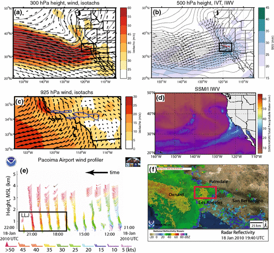
Case study analysis for the 18 January 2010 post-fire debris flow in the Station Fire burn area, western San Gabriel Mountains. Subplots show the following: a NARR 300 hPa geopotential height, wind vectors, isotachs (shaded) at 18:00 UTC. b NARR 500 hPa geopotential height, IVT > 250 kg m−1 s−1 (vectors), and IWV > 20 mm (shaded) at 18:00 UTC. Note IWV maximum over study area. Black boxes in plots a and b indicate domain shown in plot c. c 925 hPa wind vectors and isotachs (shaded) with Transverse Ranges outlined in blue at 18:00 UTC. d SSM/I IWV at 17:00 UTC, showing AR land-falling on West Coast. e Wind profiler data from Pacoima Airport 11:00 UTC-22:00 UTC with area of low-level jet boxed in black. Data provided by South Coast Air Quality Management District; base image from NOAA ESRL (2016). f High radar reflectivity over the Station Fire burn area (rough outline shown by red box) at 19:40 UTC (NCEI 2016). Similar case studies were generated for a 3-day period surrounding each of the PFDF events studied
-
2.
500 hPa height, IWV, and IVT 500 hPa heights reveal the ridge/trough pattern over the region. IWV and IVT help diagnose if an AR is present and moisture available for precipitation (Fig. 3b).
-
3.
925 hPa height, vector wind, isotachs Winds slightly above the surface at 925 hPa (~750 m) provide insight into the potential for orographic forcing and this level is close to the core altitude of water vapor transport in ARs (Fig. 3c).
-
4.
Vertical profiles of stability, moisture flux, and wind These variables are used to examine stability of the atmosphere and moisture flux. Profiles were taken at a grid point upstream (south) of each burn area and offshore in an attempt to reduce the effects of terrain-related issues in NARR and provide a full profile of the atmosphere (e.g., Fig. 6).

Composites of these variables were also generated to identify atmospheric features that have a strong signal across events. Additional data used to support case studies include radar imagery (NCEI 2016), wind profiler data (NOAA ESRL 2016) and Special Sensor Microwave Imager (SSM/I) satellite-derived IWV (CIMSS 2016).
2.3.3 Analysis of meteorological variables
For a variety of meteorological variables, NARR values were extracted for each event’s NARR time, time-3 h, and time-6 h. Variables assessed include: winds at various levels, IWV, IVT, and convective available potential energy (CAPE, a measure of buoyant energy and an indicator of potential for severe weather). Value ranges were generated based on a set of 12 NARR grid points overlying each burn area, shifted for events in different parts of the region. The values of the 12 grid points for each of the 21 events (a total of 252 values) are then aggregated, providing a range of values across all analyzed PFDF events in the Transverse Ranges.
For scalar variables such as IWV, magnitude of IVT, and CAPE, boxplots showing the median, quartiles, and outliers among values were generated for the aggregated event data. To provide additional information based on direct observation, CAPE was also composited for events using rawinsonde data from Vandenberg Air Force Base (VBG), the closest rawinsonde launch location, approximately 200 km northwest of the study area. VBG rawinsonde data are available at 00 UTC and 12 UTC and were acquired from Plymouth State (2016) upper air data archives. Data were obtained for the rawinsonde time closest to the PFDF event NARR time when possible. If rawinsonde observations were missing, then the next closest time available was used. If the NARR time for an event was 06 UTC or 18 UTC, exactly between VBG rawinsonde observations, the sounding with a higher CAPE value was used. For the vector variables wind speed and direction, wind roses were made from the aggregate event data at several different atmospheric levels.
To provide a climatological context for each event, climatologies were constructed from NARR for IVT, IWV, and CAPE. For each of the event dates, a period of ±5 days was considered, for a total period of 11 days. This was done such that each event is put in context of its particular time of year, as there may be considerable variability in the climatology of atmospheric variables within the cool season (e.g., Rutz et al. 2014). Each of the variables was then extracted from NARR for each 3-h time step in this 11-day period (88 time steps) from each year of the NARR period of record. Values were extracted at each time step for an 8 × 5 grid cell area (256 km by 160 km) overlaying the study area, and the maximum value in the grid pulled at each time step. This generated a sample size of 3256 values. Percentiles were computed from these values for each of the variables. The maximum value at the time of each PFDF event was then evaluated against the climatology to determine its percentile ranking, and the rankings are provided in “Appendix”.
3 Results and discussion
3.1 Synoptic scale features
Atmospheric rivers and their associated features as well as the common ingredients for heavy orographic precipitation were found in a majority of PFDF events. AR conditions were present during 68% of case studies and CLs occurred in 26% of events. Five events featured neither an AR nor CL (Table 2; “Appendix”).
Consistent with the dominance of AR events, compositing of IWV shows the upper three quartiles of grid points at the time of event exceed the 20 mm AR threshold (Fig. 4). Averaged across events, IWV values were in the 92nd percentile with respect to climatology (“Appendix”). For the IVT variable, the 250 kg m−1 s−1 AR threshold fell in the lower third of the lower middle quartile of the distribution at the time of event (Fig. 4). All six non-AR events had a majority of their 12 grid points at the time of event below IWV and IVT thresholds for ARs. Averaged across events, IVT values were in the 95th percentile with respect to climatology (“Appendix”). In some cases, IVT or IWV at event-3 h or event-6 h were higher than at event time (Fig. 4). An AR is typically located in the warm sector of a storm, preceding the cold front. Since many of the events exhibit lift associated with the cold front, it is possible to see convection capable of initiating a PFDF occur following the maximum values of IVT or IWV in a storm. Averaged across events, 75% of the moisture flux (product of specific humidity and wind speed) was located below 600 hPa (~4 km; Fig. 6b). This is higher in the atmosphere than in previous studies of ARs off the California coast, where 75% of moisture flux was observed below 2.25 km (Ralph et al. 2005).

Box-and-whisker plots for a composite IWV and b composite IVT from NARR data for 12 grid points pertaining to each of 21 PFDF events at NARR time of event, NARR time-3 h, and NARR time-6 h prior (n = 252 points in each box-and-whisker diagram at each time). Blue boxes indicate the two middle quartiles, red line specifies the median, and whiskers indicate the upper and lower quartiles. Red +’s specify outlier data. Green horizontal lines indicated the threshold for atmospheric river conditions for each variable based on Ralph et al. (2004) for IWV; Rutz et al. (2014) for IVT
Most events featured a neutral or negatively tilted trough (as seen in Fig. 3a, b; “Appendix”). In the case of a negatively tilted trough, instability and convection are favorable, as cold air advection occurs at upper levels above relatively warm air at low levels (MacDonald 1976). Instability can still occur within a neutral and positively tilted trough as well.
3.2 Jet position, structure, and winds
At the NARR event time, the dominant direction of the 300 hPa upper level flow over the composited study areas was southwest to west-southwest (Fig. 5, top; “Appendix”). All observations fell between 185° and 285°, with 90% of observations falling between 215° and 275°. In a majority of observations (67%), the average speed of the 300 hPa flow over the area of interest was ≥40 m s−1, indicative of a weak of a weak to moderate flow aloft. Several of the events examined see 300 hPa wind speeds in excess of 50 m s−1, indicating moderate to strong flow. The velocity of the upper level winds indicates the strength of the upper level divergence, which promotes upward vertical motions and potential for precipitation (Clark et al. 2009; O’Hara et al. 2009).

Wind rose diagrams for composite 300 hPa wind (top row), 700 hPa wind (middle row) and 925 hPa wind (bottom row) from NARR data for 12 grid points pertaining to each of 21 PFDF events at NARR time of event, 3 h prior, and 6 h prior (n = 252 points in each rose at each time). Total length of each bar indicates the frequency of grid points with wind in that particular direction. Length of colored areas within bar indicates the frequency of wind at a particular speed in that direction
The position of the upper level jet was to the south of the region of interest in a majority of events (68%; Table 2), typically placing the Transverse Ranges in the curved jet exit and/or the left exit of a jet streak, an area associated with strong upper level divergence and lift, as shown in Fig. 3a. This is consistent with the “southerly displaced jet stream” cited by Tarleton and Kluck (1994) as a typical feature in extreme precipitation events in California. In several cases (26%), the upper level jet was directly over the study area, and finer scale splitting within the jet developed entrance or exit regions over the study area favorable for upper level divergence. In only one case, the upper level jet was located to the north of the region, though was positioned such that the right entrance of the jet was over the Transverse Ranges.
At mid-levels (700 hPa), winds were predominantly from the southwest at the time of the event, with 69% of observations falling between 205° and 245° (Fig. 5, middle row). The predominant speed was 15–20 m s−1 (38%); and 37% of observations were greater than 20 m s−1. From NARR time-6 h through NARR time of event, wind speeds increased and direction became more uniformly from the southwest.
At low levels (925 hPa), wind direction was predominantly from 155° to 215° (60% of observations; Fig. 5 bottom row and “Appendix”). The dominant speed was 5–10 m s−1 (49%), with 8% of observations exceeding 15 m s−1. This is significant in that the low-level moderate intensity southerly winds are orthogonal to the east-to-west oriented Transverse Ranges, providing one of the necessary conditions for heavy orographic precipitation (Lin et al. 2001).
Wind profiler data (NOAA ESRL 2016; as in Fig. 3e) were used to diagnose the presence of LLJs for events when data were available. Profiler data were available for the ten post-2005 events, though available locations were inconsistent. Profiler data confirmed the presence of LLJs in the seven of these events; six of which were AR events. No LLJ was detected in three of the four non-AR events in this period (“Appendix”).
3.3 Atmospheric stability
Stability profiles below ~3 km (700 hPa) as observed in vertical profiles could be broadly divided into weakly unstable, moist neutral, or unstable near surface becoming moist neutral with height (Table 2; “Appendix”). A large majority of the events showed moist-neutral stability either in all levels below 3 km or in the 1–2+ km layer (Fig. 6a). Moist-neutral stability is recognized as little or no change in θ e* with height \(\left({{\partial \theta_{e*} /\partial {{z}}}} = 0\right)\). The significance of moist neutrality is that if the parcel is displaced upward, it will maintain its new position. Air parcels in a neutral setting can be forced to ascend relatively easily in the presence of a lifting mechanism such as a cold front or mountain barrier, resulting in convection. Moist-neutral stability is a common feature of ARs (Ralph et al. 2005). Several events saw instability at low levels (\({{\partial \theta_{e*} /\partial {{z}}}} \, <\, 0\); Fig. 6a) transitioning to moist neutral near 1 km, distinct from the moist-neutral layer observed from the surface to 2.8 km in a composite of AR events presented by Ralph et al. (2005).

a Moist stability profile for 19 PFDF events and b moisture flux profile for 19 PFDF events based on NARR data at NARR event time. In plot a, values close to 0 correspond to moist-neutral conditions
The scale for CAPE begins at 0, and higher values of CAPE indicate greater instability and severe weather. In the CAPE climatologies created for periods relative to the PFDF events studied here, a CAPE value of 100 J kg−1 was on average the 85th percentile for the maximum values in the study area (“Appendix”). At the NARR event time, median NARR CAPE was 20 J kg−1 and ranged from 0 to 1330 J kg−1, with the values exceeding 500 J kg−1 all coming from grid points associated with the two Springs Fire cases in the Santa Monica Mountains. At the time closest to the event, median CAPE from the VBG soundings was 40 J kg−1 and ranged from 0 to 463 J kg−1 (Fig. 7; “Appendix”). A general trend of increasing CAPE was observed in NARR in the 3-h and 6-h time steps leading up to the event (Fig. 7).

Box-and-whisker plots for composite CAPE from NARR data for 12 grid points pertaining to each of 21 PFDF events at NARR time of event, NARR time-3 h, and NARR time-6 h prior (n = 252 points in each box-and-whisker diagram at each time). Blue boxes indicate the two middle quartiles, red line specifies the median, and whiskers indicate the upper and lower quartiles. Red +’s specify outlier data. The second from left box and whisker in each plot represents the values acquired for rawinsonde soundings at Vandenberg AFB at closest time available to each event; as the sounding produces a single value, there is one value for each event date and n = 19
3.4 Analysis of radar imagery
Radar imagery was available for 14 unique PFDF event dates through NCEI’s Radar Data Map (https://gis.ncdc.noaa.gov/maps/ncei/radar). All events had radar returns of at a minimum 50 dBZ (approximately >48 mm h−1; as in Fig. 3f),Footnote 1 indicative of heavy precipitation. Six of the 14 events had very strong returns over 60 dBZ (>200 mm h−1), indicative of very intense precipitation. Narrow cold frontal rain bands (NCFRs) were identified in five of the 14 events (Table 2; “Appendix”; example in Fig. 8). NCFRs show up in radar imagery as a narrow band of high radar reflectivity on the order of 200 km long with breaks and gaps along their length (Fig. 8; Jorgensen et al. 2003). The five NCFRs in this study all followed a similar west-to-east path across the southern California Bight with the northern half of the NCFR situated over land, while the southern half was over water and the feature’s long axis perpendicular to the coast. This preferential orientation likely occurs due to blocking and modification of the low-level front by coastal terrain (Neiman et al. 2004; Hughes et al. 2009).

Radar image of a narrow cold frontal rain band (NCFR) passing over the Transverse Range study area during the 06 February 1998 PFDF event in the Grand/Hopper burn areas in the Topatopa Mountains
Radar imagery associated with one PFDF event on 12 November 2009 resulted from the development of a very isolated convective cell in the San Gabriel Mountains, reminiscent of a warm season thunderstorm event. The remaining eight of the 14 PFDF events for which radar data were available featured other types of convective activity such as orographic forcing and mesoscale rain bands (as in Fig. 3f) that are not discussed in detail within this paper.
3.5 Tools and applications
The prominence of ARs and their related features in the occurrence of PFDFs in the Transverse Ranges suggests that those concerned with PFDFs will benefit from incorporating the use of online AR forecast and diagnostic tools into their decision-making. One such tool is the US West Coast AR Landfall Tool available through the Center for Western Weather and Water Extremes (CW3E) at http://cw3e.ucsd.edu/?page_id=491. This tool provides a 16-day forecast where the user can see the probability, magnitude, location, and timing of AR conditions arriving along the West Coast as well as how AR conditions vary in a forecast model through time. Proper use of this tool among others can generate awareness of the potential for a PFDF and support planning and decision-making in both research and emergency response. Additionally, the IVT variable assessed in the aforementioned AR forecasting tool has been shown to be more successful in long-range forecasts than precipitation (Lavers et al. 2016). Thus, forecasts of IVT can be used to provide forecasts of likelihood for heavy rainfall with greater certainty further ahead than the traditional precipitation forecasts.
3.6 Limitations and future work
Limitations of this study lie in NARR’s 32 km resolution and thus its inability to resolve fine-scale processes important to the development of convective cells such as blocking, barrier jet features, and low-level convergence along terrain barriers that are common in the region (Small 1999; Neiman et al. 2004; Hughes et al. 2009). Additionally, Hughes et al. (2012) have noted challenges in how NARR represents low-level winds and winds at the land-sea boundary, which may impact results for winds at these levels. The coarseness of the NARR data may also impact the accuracy of estimates of stability. CAPE, for example, can vary greatly in the course of a storm event. Sukup et al. (2016) show a significant increase in CAPE following a frontal passage after the PFDF had already occurred during the 12 December 2014 PFDF event. Thus, it is possible that with the spatial and temporal coarseness of both NARR and radiosonde data stability variables assessed are not representative of the true event time and may be biased high or low based on times available.
While AR conditions make up a majority of cool season PFDF events in this study, there are, on occasion, isolated thunderstorm events such as the 12 November 2009 PFDF event included herein. Thus, we advise that all storm types should be considered in emergency preparedness; however, advantage should be taken of recent advancements in AR detection and prediction given the dominance of ARs among the PFDF cases explored in this study.
This work is, in essence, an analysis of cases of intense precipitation in the Transverse Ranges, subset by PFDF occurrence. A broader approach would be to look at all precipitation events over a particular threshold in the region. However, PFDF thresholds have been noted to vary in space (Staley et al. 2016) thus choosing one representative threshold may not suffice. Focusing on events known to produce impactful PFDFs ensures precipitation was indeed sufficient. Additionally, applying meteorological analyses to verified impactful PFDF events allows us to make a direct connection with the experiences and concerns of our target audience in a way that a more abstract approach of exploring precipitation over a particular intensity may not.
The lack of observations of both post-fire debris flow activity and precipitation limits the assessment of null events. Without a high-resolution network of gauges and instruments that can record debris flow response and triggering rainfall within the burn area, it is difficult to determine whether precipitation of sufficient intensity and duration for PFDF activity did or did not fall on a burn area. In cases outside of research efforts that utilize instrumentation, PFDFs are often only noted if they impact human infrastructure. Thus, if a PFDF occurred in an inaccessible remote area of a watershed, it may not be documented. In the null case most relevant to this work (all favorable synoptic-scale conditions present, but intense precipitation does not occur, field observations made, and no PFDFs present), analysis using mesoscale modeling would be needed to assess why intense cells did not develop, which is beyond the scope of this work. Thus, this work focuses on well-documented damaging debris flows that affected structures or infrastructure downstream of the burned watershed.
A major challenge that remains in this research topic is identifying the exact timing and location where intense convective cells might develop (isolated or within a larger storm system). Similar to the suggestions of Moody et al. (2013) and Shakesby et al. (2016), we propose future work should focus on high-resolution (≤1 km) modeling of the region to identify favored areas for intense convection under a variety of flow regimes. For modeling efforts to be successful, precise timing of a greater number of PFDF events is necessary. There are many challenges to overcome in instrumenting basins, as described in Kean et al. (2011) and Staley et al. (2013), but, where present, we have found this timing data essential to assessment of the meteorological component of PFDF events.
4 Conclusions
A catalog of 93 individual post-fire debris flow (PFDF) events associated with 19 precipitation events was compiled for the Transverse Ranges using a variety of resources. Meteorological case studies were created for each event using hourly precipitation data from various weather stations, the North American Regional Reanalysis (NARR) dataset, radar imagery, wind profiler data, and rawinsonde observations.
The majority of the precipitation events producing PFDFs are moderate to strong in terms of moisture transport; 11 of 19 events have IVT ≥ 95th percentile for the location and time of year. A few of the events examined have weaker moisture transport (<90th percentile), though these events feature instability that is characteristic of only a few of the high IVT events. Thus, there is some variability in the synoptic-scale characteristics of precipitation events that produce PFDFs. However, we do find a set of characteristics that are common across a majority of PFDF events. These common atmospheric conditions associated with cool season PFDFs can be summarized as:
-
Atmospheric rivers (ARs) were present in 13 of 19 PFDF events (9 had AR only, 4 had AR and a closed low)
-
All 13 AR events featured IVT ≥ 90th percentile and 8 had IVT in the 99th percentile (strong events for the location and time of year)
-
On average, 75% of moisture flux in PFDF events below 4 km
-
Closed lows (CL) were present in 5 of 19 PFDF events (1 had CL only, 4 had AR and CL)
-
Neither AR nor CL conditions were present in 5 events
-
Moderate to strong flow aloft: Upper level (300 hPa) west-southwest flow typically >40 m s−1
-
Upper level jet position in majority of events (13 of 19) is displaced to south such that the Transverse Ranges lie in divergent jet exit, an area favorable for upward vertical motions
-
Presence of moderate speed (5–10+ ms−1) southerly winds below 1 km
-
Predominantly moist-neutral stability (AR feature), especially in the 1–2+ km layer; in some cases weakly unstable at low levels
-
Median CAPE of 20–40 J kg−1 at time of event with a range from 0 to 1300 J kg−1 among events
-
High radar returns (>50 dBz); in several cases narrow cold frontal rainbands
Together, these common conditions provide a general picture of the synoptic-scale atmospheric phenomena present in storms that trigger PFDFs and provide the framework for a conceptual cool season model, illustrated in Fig. 9.

Conceptual model of common features associated with PFDF in the Transverse Ranges at various scales. This represents the majority of events, which feature atmospheric rivers and their associated characteristics, but does not capture all variability seen among events. a Depicts the synoptic scale features and typical positions. b Provides a mesoscale perspective of the events in association with the burn areas and depicts a cold front moving into the region, which acts as a lifting mechanism for the NCFR events, and potentially others. c Depicts a conceptual cross-section of a storm event impacting the study area. Vertical profiles on the lefthand side of the figure show moisture flux is present primarily in low levels, and a generally moist-neutral stability profile indicates little resistance to orographic lift. Other lifting mechanisms may be at work as well; see Sect. 1.2. Moisture flux and stability profiles as well as wind profile are composites of NARR data for all 19 post-fire debris flow events. Schematic in c designed after Ralph et al. (2005)
The results presented here reinforce NWS forecaster experience pertaining to PFDF events (Cannon et al. 2010; Sukup et al. 2016) as well as illustrate and quantify these relationships. They also provide information on the variability of conditions observed among PFDF events that may be helpful in forecasting. The results of this study assist those evaluating runoff hazards in burned areas, as well as emergency managers, research geologists and hydrologists by going beyond the common descriptor of “intense convection” cited as the cause of PFDF events and identifying broad scale features that can be recognized in forecast models with more advanced notice than convective cells. Improved understanding by these groups can help build awareness of the likelihood of PFDF events with more lead time and may improve interpretation and decision-making related to NWS forecasts, watches, and warnings.
Notes
Rain rates based on Marshall and Palmer (1948). Note values given for rain rate are instantaneous corresponding to the imagery and do not represent the actual value observed over the course of an hour.
Abbreviations
- LST:
-
Local standard time
- UTC:
-
Coordinated universal time
- PFDF:
-
Post-fire debris flow
- I–D :
-
Intensity–duration
- AR:
-
Atmospheric river
- CL:
-
Closed low
- ARCL:
-
Both AR and CL
- OTH:
-
Other atmospheric feature
- IWV:
-
Integrated water vapor
- IVT:
-
Integrated water vapor transport
- NCFR:
-
Narrow cold frontal rain band
- NARR:
-
North American Regional Reanalysis
- LLJ:
-
Low-level jet
- CAPE:
-
Convective available potential energy
- VBG:
-
Vandenberg, California
- CW3E:
-
Center for Western Weather and Water Extremes
References
ABC7 News (2014) Nov 2 2014: Camarillo Springs evacuation order lifted after debris flow. http://abc7.com/weather/1-rescued-residents-evacuated-after-camarillo-mudslide/376277/. Accessed 10 Feb 2016
Browning KA, Pardoe CW (1973) Structure of low-level jet streams ahead of mid-latitude cold fronts. Q J R Meteorol Soc 99(422):619–638
California Department of Forestry and Fire Protection (CALFIRE) (2014) Fire perimeters, Version14_2. http://frap.cdf.ca.gov/data/frapgisdata-sw-fireperimeters_download. Accessed 12 Mar 2016
California Office of Emergency Services (2010) 2010 January statewide winter storms after action/corrective action report. http://www.caloes.ca.gov/PlanningPreparednessSite/Documents/08%20January2010%20Statdewide%20Rains%20Exec%20Summary%20and%20report2.pdf. Accessed 10 Feb 2016
Cannon SH, Gartner JE, Wilson RC, Bowers JC, Laber JL (2008) Storm rainfall conditions for floods and debris flows from recently burned areas in southwestern Colorado and southern California. Geomorphology 96(3):250–269
Cannon SH, Boldt EM, Kean JW, Laber JL, Staley DM (2010) Relations between rainfall and postfire debris-flow and flood magnitudes for emergency-response planning, San Gabriel Mountains, southern California. U.S. Geological survey open–file report 2010-1039, pp 31
Carlson TN (1998) Mid-latitude weather systems. American Meteorological Society, Boston, p 507
CBS Los Angeles (2014) Nov 1 2014: Major debris flow forces evacuation of 11 Camarillo Springs Homes. http://losangeles.cbslocal.com/2014/11/01/major-debris-flow-forces-evacuation-of-11-camarillo-springs-homes/. Accessed 12 Mar 2016
Chawner WD (1935) Alluvial fan flooding: the Montrose, California, flood of 1934. Geogr Rev 25(2):255–263
Chin EH, Aldridge BN, Longfield RJ (1991) Floods of February 1980 in southern California and central Arizona. US Geol Surv Prof Pap 1494:126
CIMSS (2016). Morphed integrated microwave imagery at CIMSS—total precipitable water (MIMIC—TPW). http://tropic.ssec.wisc.edu/real-time/mimic-tpw/epac/main.html. Accessed 20 Mar 2016
City of Sierra Madre Blog (2009) February 2009 emergency information by Sierra Madre PIO. http://sierramadrepio.blogspot.com/2009_02_01_archive.html. Accessed 10 Feb 2016
Clark AJ, Schaffer CJ, Gallus WA Jr, Johnson-O’Mara K (2009) Climatology of storm reports relative to upper-level jet streaks. Weather Forecast 24(4):1032–1051
County of Ventura (2015) Multi-hazard Mitigation Plan: September 2015, pp 718. http://www.vcfloodinfo.com/pdf/2015%20Ventura%20County%20MultiHazard%20Mitigation%20Plan%20and%20Appendices.pdf. Accessed 12 Jan 2016
Daily Mail UK (2014) 14 Dec 2014: the street that was buried by a mudslide. http://www.dailymail.co.uk/news/article-2873433/Devastation-California-mudslide-seen-air-boulder-strewn-rivers-mud-swept-hillsides-submerged-homes.html. Accessed 12 Jan 2016
DeBano LF (1981) Water repellent soils; a state-of-the-art. Forest service; general technical report no. PSW-46. Pacific Southwest Forest and Range Experiment Station
DeBano LF (2000) The role of fire and soil heating on water repellency in wildland environments: a review. J Hydrol 231–232:195–206
Dettinger MD, Ralph FM, Das T, Neiman PJ, Cayan DR (2011) Atmospheric rivers, floods and the water resources of California. Water 3(2):445–478
Eaton EC (1936) Flood and erosion control problems and their solution. Trans Am Soc Civ Eng 101(1):1302–1330
Gartner JE, Bigio ER, Cannon SH (2004) Compilation of post wildfire runoff-event data from the Western United States. US geological survey open-file report 04-1085
Gartner JE, Cannon SH, Santi PM, Dewolfe VG (2008) Empirical models to predict the volumes of debris flows generated by recently burned basins in the western U.S. Geomorphology 96:339–354
Gartner JE, Cannon SH, Santi PM (2014) Empirical models for predicting volumes of sediment deposited by debris flows and sediment-laden floods in the Transverse Ranges of southern California. Eng Geol 176:45–56
Guzzetti F, Peruccacci S, Rossi M, Stark CP (2008) The rainfall intensity–duration control of shallow landslides and debris flows: an update. Landslides 5(1):3–17
Hobbs PV (1978) Organization and structure of clouds and precipitation on the mesoscale and microscale in cyclonic storms. Rev Geophys 16(4):741–755
Hobbs PV, Persson POG (1982) The mesoscale and microscale structure and organization of clouds and precipitation in midlatitude cyclones. Part V: the substructure of narrow cold-frontal rainbands. J Atmos Sci 39(2):280–295
Hughes M, Hall A, Fovell RG (2009) Blocking in areas of complex topography, and its influence on rainfall distribution. J Atmos Sci 66(2):508–518
Hughes M, Neiman PJ, Sukovich E, Ralph M (2012) Representation of the Sierra Barrier Jet in 11 years of a high-resolution dynamical reanalysis downscaling compared with long-term wind profiler observations. J Geophys Res 117:D18116. doi:10.1029/2012JD017869
Jorgensen DP, Pu Z, Persson POG, Tao WK (2003) Variations associated with cores and gaps of a Pacific narrow cold frontal rainband. Mon Weather Rev 131(11):2705–2729
Jorgensen DP, Hanshaw MN, Schmidt KM, Laber JL, Staley DM, Kean JW, Restrepo PJ (2011) Value of a dual-polarized gap-filling radar in support of southern California post-fire debris-flow warnings. J Hydrometeorol 12(6):1581–1595
Kalnay E, Kanamitsu M, Kistler R, Collins W, Deaven D, Gandin L et al (1996) The NCEP/NCAR 40-year reanalysis project. Bull Am Meteor Soc 77(3):437–471
Kean JW, Staley DM, Cannon SH (2011) In situ measurements of post-fire debris flows in southern California: comparisons of the timing and magnitude of 24 debris-flow events with rainfall and soil moisture conditions. J Geophys Res Earth Surf 116:F04019
Keeley JE, Fotheringham CJ, Moritz MA (2004) Lessons from the October 2003 wildfires in southern California. J Forest 102(7):26–31
Lavers DA, Waliser DE, Ralph FM, Dettinger MD (2016) Predictability of horizontal water vapor transport relative to precipitation: enhancing situational awareness for forecasting Western US extreme precipitation and flooding. Geophys Res Lett 43(5):2275–2282
Lin YL, Chiao S, Wang TA, Kaplan ML, Weglarz RP (2001) Some common ingredients for heavy orographic rainfall. Weather Forecast 16(6):633–660
Los Angeles Times Blog, Groves M (2009) 06 February 2009 Mud mucks up streets in Sylmar. http://latimesblogs.latimes.com/.m/lanow/2009/02/mud-flow-mucks.html. Accessed 20 Jan 2016
Los Angeles Times, Lin II RG, Kim V, Vives R (2010) 07 February 2010: Niagara of mud hits homes. http://articles.latimes.com/2010/feb/07/local/la-me-rain7-2010feb07. Accessed 20 Jan 2016
MacDonald NJ (1976) On the apparent relationship between convective activity and the shape of 500 mb troughs. Mon Weather Rev 104(12):1618–1622
Marshall JS, Palmer WMK (1948) The distribution of raindrops with size. J Meteorol 5(4):165–166
Mesinger F, DiMego G, Kalnay E, Mitchell K, Shafran PC, Ebisuzaki W et al (2006) North American regional reanalysis. Bull Am Meteor Soc 87(3):343–360
Monteverdi JP (1995) Overview of the meteorology of rain events in California. California Extreme Precipitation In: Symposium proceedings. http://cepsym.org/Sympro1995/monteverdi.pdf. Accessed 14 Mar 2016
Moody JA, Shakesby RA, Robichaud PR, Cannon SH, Martin DA (2013) Current research issues related to post-wildfire runoff and erosion processes. Earth-Sci Rev 122:10–37
Moore BJ, Neiman PJ, Ralph FM, Barthold F (2012) Physical processes associated with heavy flooding rainfall in Nashville, Tennessee and vicinity during 1-2 May 2010: the role of an atmospheric river and mesoscale convective systems. Mon Weather Rev 140:358–378
National Centers for Environmental Information (2016) Radar data map, National Reflectivity Mosaic. https://gis.ncdc.noaa.gov/maps/ncei/radar. Accessed 20 Jan 2016
Neary DG, Klopatek CC, DeBano LF, Folliott PF (1999) Fire effects on belowground sustainability: a review and synthesis. J For Ecol Manag 122:51–71
Neiman PJ, Ralph FM, White AB, Kingsmill DE, Persson POG (2002) The statistical relationship between upslope flow and rainfall in California’s coastal mountains: observations during CALJET. Mon Weather Rev 130(6):1468–1492
Neiman PJ, Ralph FM, Persson POG, White AB, Jorgensen DP, Kingsmill DE (2004) Modification of fronts and precipitation by coastal blocking during an intense landfalling winter storm in southern California: observations during CALJET. Mon Weather Rev 132(1):242–273
Neiman PJ, Ralph FM, Wick GA, Lundquist JD, Dettinger MD (2008) Meteorological characteristics and overland precipitation impacts of atmospheric rivers affecting the West Coast of North America based on eight years of SSM/I satellite observations. J Hydrometeorol 9(1):22–47
NOAA Earth System Research Laboratory (ESRL; 2016) NOAA ESRL GSD-MADIS CAP profiler real time data display. https://madis-data.noaa.gov/cap/profiler.jsp?view=swus. Accessed 10 Jan 2016
NOAA Hydrometeorological Design Studies Center (HDSC; 2017) NOAA Atlas 14 point precipitation frequency estimates. http://hdsc.nws.noaa.gov/hdsc/pfds/. Accessed 24 Jan 2017
NOAA-USGS Debris Flow Task Force (2005) NOAA-USGS debris-f low warning system: Final report. U.S. geological survey circular 1283. http://pubs.usgs.gov/circ/2005/1283/pdf/Circular1283.pdf Accessed 20 Aug 2016
NASA Earth Observatory (2003). Fires in southern California. http://earthobservatory.nasa.gov/NaturalHazards/view.php?id=12373&eocn=image&eoci=morenh. Accessed 1 May 2016
Oakley NS, Redmond KT (2014) A climatology of 500-hPa closed lows in the Northeastern Pacific Ocean, 1948–2011. J Appl Meteorol Climatol 53(6):1578–1592
O’Hara BF, Kaplan ML, Underwood SJ (2009) Synoptic climatological analyses of extreme snowfalls in the Sierra Nevada. Weather Forecast 24(6):1610–1624
Parise M, Cannon SH (2012) Wildfire impacts on the processes that generate debris flows in burned watersheds. Nat Hazards 61(1):217–227
Plymouth State University (2016) Plymouth State weather center. http://vortex.plymouth.edu/. Accessed 12 Mar 2016
Ralph FM, Dettinger MD (2012) Historical and national perspectives on extreme West Coast precipitation associated with atmospheric rivers during December 2010. Bull Am Meteor Soc 93(6):783–790
Ralph FM, Neiman PJ, Wick GA (2004) Satellite and CALJET aircraft observations of atmospheric rivers over the eastern North Pacific Ocean during the winter of 1997/98. Mon Weather Rev 132(7):1721–1745
Ralph FM, Neiman PJ, Rotunno R (2005) Dropsonde observations in low-level jets over the northeastern Pacific Ocean from CALJET-1998 and PACJET-2001: mean vertical-profile and atmospheric-river characteristics. Mon Weather Rev 133(4):889–910
Ralph FM, Neiman, PJ, Wick GA, Gutman SI, Dettinger MD, Cayan DR, White AB (2006) Flooding on California’s Russian river: role of atmospheric rivers. Geophys Res Lett 33(13):L13801
Ralph FM, Coleman T, Neiman PJ, Zamora R, Dettinger MD (2013) Observed impacts of duration and seasonality of atmospheric-river landfalls on soil moisture and runoff in coastal northern California. J Hydrometeor 14:443–459
Ralph FM, Prather KA, Cayan D, Spackman JR, DeMott P, Dettinger M, Fairall C, Leung R, Rosenfeld D, Rutledge S, Waliser D, White AB, Cordeira J, Martin A, Helly J, Intrieri J (2016) CalWater field studies designed to quantify the roles of atmospheric rivers and aerosols in modulating U.S. West Coast precipitation in a changing climate. Bull Am Meteorol Soc 97:1209–1228
Raphael MN (2003) The Santa Ana winds of California. Earth Interact 7(8):1–13
Riggan PJ, Lockwood RN, Lopez EN (1985) Deposition and processing of airborne nitrogen pollutants in Mediterranean-type ecosystems of southern California. Environ Sci Technol 19(9):781–789
Rutz JJ, Steenburgh WJ, Ralph FM (2014) Climatological characteristics of atmospheric rivers and their inland penetration over the western United States. Mon Weather Rev 142(2):905–921
San Bernardino Sun (1980a) 10 January 1980: heavy rain causes havoc. https://www.newspapers.com/newspage/62887387/. Accessed 20 Jan 2016
San Bernardino Sun (1980b) 06 April 1980: the storms of winter: an overview. https://www.newspapers.com/newspage/62867758/. Accessed 20 Jan 2016
San Bernardino Sun (1980c) 29 January 1980: Mud threatens S.B. homes again https://www.newspapers.com/newspage/62881718/. Accessed 20 Jan 2016
San Bernardino Sun (1980d) 17 February 1980: Downpours force more evacuations. https://www.newspapers.com/newspage/62648829/. Accessed 20 Jan 2016
Santi PM, Morandi L (2012) Comparison of debris-flow volumes from burned and unburned areas. Landslides 10(6):757–769
Schleiss AJ, de Cesare G, Franca MJ, Pfister M (2014) Reservoir sedimentation. CRC Press, London, p 300
Shakesby RA, Moody JA, Martin DA, Robichaud PR (2016) Synthesising empirical results to improve predictions of post-wildfire runoff and erosion response. Int J Wildland Fire 25(3):257–261
Shuirman G, Slosson JE (1992) Forensic engineering: environmental case histories for civil engineers and geologists. Academic Press, Cambridge
Slosson JE, Havens GW, Shuirman G, Slosson TL (1991) Harrison Canyon debris flows of 1980. Environ Geol Water Sci 18(1):27–38
Small IJ (1999) An observational study of a California Bight coastal convergence zone produced by flow interaction with mainland topography: precipitation producer in southern California. NOAA Technical Attachment No. 99-19. http://www.wrh.noaa.gov/media/wrh/online_publications/TAs/ta9919.pdf. Accessed 15 Apr 2016
Staley DM, Kean JW, Cannon SH, Schmidt KM, Laber JL (2013) Objective definition of rainfall intensity–duration thresholds for the initiation of post-fire debris flows in southern California. Landslides 10(5):547–562
Staley DM, Negri JA, Kean JW, Laber JL, Tillery AC, Youberg AM (2016) Prediction of spatially explicit rainfall intensity–duration thresholds for post-fire debris-flow generation in the western Unites States. Geomophology 278(2017):149–162
Sukup SJ, Laber J, Sweet D, Thompson R (2016) Analysis of an intense narrow cold frontal rainband and the springs fire debris flow of 12 December 2014. NWS technical attachment 1601. http://www.wrh.noaa.gov/media/wrh/online_publications/TAs/TA1601.pdf. Accessed 15 Jan 2016
Tarleton LF, Kluck DR (1994) Analysis of major storms in southern California. In: California extreme precipitation symposium proceedings. http://cepsym.org/Sympro1994/tarleton.pdf. Accessed 14 Mar 2016
Taylor DB (1982) Floodflows in major streams in Ventura County. In: Brooks NH (ed) Storms, floods, and debris flows in southern California and Arizona 1978 and 1980: proceedings of a symposium, September 17–18, 1980. National Academy Press, p 487
Troxell HC, Petersen JQ (1937) Flood in La Canada Valley, California January 1, 1934: U.S. geological survey water-supply paper 796-C, p 98
United States Geological Survey (2005) Southern California—wildfires and debris flows. USGS Fact Sheet 2005-3106. http://pubs.usgs.gov/fs/2005/3106/. Accessed 10 Jan 2016
URS Corporation (2005) Flood Mitigation Plan for Ventura County, California: URS Corporation, p 128. http://www.ventura.org/wcvc/documents/PDF/floodmitigationplan2005.pdf. Accessed 12 Jan 2016
Weaver RL (1962) Meteorology of hydrologically critical storms in California. Hydrometeorological Report 37. US Dept. of Commerce
Wells II WG (1987) The effects of fire on the generation of debris flows in southern California. In: Costa JE, Wieczorek GF (eds) Debris flows/avalanches—process, recognition, and mitigation: Geological Society of America, Reviews in Engineering Geology VII, pp 105–114
Wells WG II (1981) Some effect of brushfires on erosion processes in coastal southern California. In: Davies TRH, Pearce AJ (eds), Erosion and sediment transport in pacific rim Steeplands, January 1981, Chirst Church, New Zealand. Sponsored jointly by the Royal Society of New Zealand, New Zealand Hydrological Society, IAHS, and the National Water and Soil Conservation Authority of New Zealand. International Association of Hydrologic Sciences Publication, vol 132, pp 305–342
Zhu Y, Newell RE (1998) A proposed algorithm for moisture fluxes from atmospheric rivers. Mon Weather Rev 126(3):725–735
Acknowledgements
This work was supported by the Center for Western Weather and Water Extremes at Scripps Institution of Oceanography as part of the California Department of Water Resources Alluvial Fan Flooding project, California Natural Resources Agency contract #4600010378. Oakley was additionally supported by a fellowship from Nevada NASA Space Grant #NNX10AN23H. We would like to thank NWS Oxnard for providing background and insights for this work, Dennis Staley at USGS for providing debris flow trigger times for several events in the Station Fire burn area, and three anonymous reviewers for their helpful comments which improved this manuscript.
Author information
Authors and Affiliations
Corresponding author
Appendix
Rights and permissions
Open Access This article is distributed under the terms of the Creative Commons Attribution 4.0 International License (http://creativecommons.org/licenses/by/4.0/), which permits unrestricted use, distribution, and reproduction in any medium, provided you give appropriate credit to the original author(s) and the source, provide a link to the Creative Commons license, and indicate if changes were made.
About this article

Cite this article
Oakley, N.S., Lancaster, J.T., Kaplan, M.L. et al. Synoptic conditions associated with cool season post-fire debris flows in the Transverse Ranges of southern California. Nat Hazards 88, 327–354 (2017). https://doi.org/10.1007/s11069-017-2867-6
Received:
Accepted:
Published:
Issue Date:
DOI: https://doi.org/10.1007/s11069-017-2867-6