
Abstract
The novel coronavirus disease, which originated in Wuhan, developed into a severe public health problem worldwide. Immense stress in the society and health department was advanced due to the multiplying numbers of COVID carriers and deaths. This stress can be lowered by performing a high-speed diagnosis for the disease, which can be a crucial stride for opposing the deadly virus. A good large amount of time is consumed in the diagnosis. Some applications that use medical images like X-Rays or CT-Scans can pace up the time used in diagnosis. Hence, this paper aims to create a computer-aided-design system that will use the chest X-Ray as input and further classify it into one of the three classes, namely COVID-19, viral Pneumonia, and healthy. Since the COVID-19 positive chest X-Rays dataset was low, we have exploited four pre-trained deep neural networks (DNNs) to find the best for this system. The dataset consisted of 2905 images with 219 COVID-19 cases, 1341 healthy cases, and 1345 viral pneumonia cases. Out of these images, the models were evaluated on 30 images of each class for the testing, while the rest of them were used for training. It is observed that AlexNet attained an accuracy of 97.6% with an average precision, recall, and F1 score of 0.98, 0.97, and 0.98, respectively.
1 Introduction
The World Health Organization (WHO), on 30 January 2020, had announced the breakout of the novel coronavirus disease as a “Public Health Emergency of International Concern” [43]. COVID-19 was the name given by the World Health Organization (WHO) on 11 February 2020 [8]. The novel coronavirus (COVID-19) depiction started with the discovery of Pneumonia with unseen causes in late December 2019 in Wuhan, Hubei province of China, and has developed into a severe public health problem all over the world [5, 9, 33, ] and has swiftly become a pandemic [11, 30, 36, 46]. The Covid19 widespread was found to cause a virus named severe acute respiratory syndrome coronavirus two, also called SARS-CoV-2 [8, 12, 28, 34]. Coronaviruses (CoV) are a large family of perilous viruses [15] that becomes the source of illnesses ranging from colds to more severe pathologies [8, 38]. The Middle East Respiratory Syndrome Coronavirus(MERS-CoV) and Severe Acute Respiratory Syndrome Coronavirus (SARS-CoV) had caused severe respiratory diseases and deaths in humans [30]. The coronaviruses were named so because when they were examined under an electron microscope, the shape of the virus was like a solar corona, which is crown-like in shape [15]. The presence of COVID-19 was not found previously at any point in time; it was the first time in 2019 that it was discovered. It affects the animals, but due to its zoonotic nature, it has also shown the potential to get transferred among humans as well [12]. Some recent findings suggest that the SARS-CoV virus is contaminated from musk cats to humans, while the MERS-CoV is contaminated from dromedary to humans. The contamination of the COVID-19 has been believed to be passed from bats to humans [28].
The interval between the contamination and the emergence of the first COVID-19 symptoms can stretch up to 15 days. Hence the infected ones are affecting the healthy ones without even realizing thereby spreading the virus more broadly. Two hundred twelve countries were facing covid19 infected people cases just after a few weeks of its confirmation in Wuhan [8, 19, 34]. When this document came in, the total confirmed coronavirus cases had reached 66,598,716, including the 1,530,650 deaths and 46,065,766 recovered cases [8].
The typical clinical features and signs of infections include fever, dry cough, sore throat, headache, fatigue, shortness of breath, muscle pain, loss of smell without any nasal obstruction, including the disappearance of taste. For more serious conditions, this infection can cause respiratory difficulties, Pneumonia, septic shock, and multi-organ failure, leading to hospitalization and, unfortunately, death [8, 19, 28, 34].
The transmission of the disease itself makes it more dangerous. It only requires droplets secreted while talking, sneezing, coughing, etc., for transmitting the disease to another person. Hence the ones inside the proximity of an infected person get higher the chances of getting infected. [8, 9, 19, 38, 41].
The whole world is waiting for the vaccine while following the precautions as advised by the World Health Organisation. These precautions include frequent handwashing with soap, maintaining social distance, covering mouth with handkerchief or elbow while coughing or sneezing, not touching eyes, mouth, or nose, and wearing a mask in any case [8]. Many countries have posed lockdown to avoid further spread and minimized their residents’ movements inside and in between cities and countries [8, 9, 33].
Since COVID-19 was a new virus, there was a shortage of testing kits for tracking the spread of the disease among humans. The existing procedures took a considerable amount of time, which was not enough to cope with the demand at that point, like Reverse Transcription Polymerase Chain Reaction (RT-PCR), which was the most concrete test available to detect the virus. RT-PCR took more than 24 hours and, in the worst cases few days. The tests were accurate on the trade-off with the time consumed for testing any patient’s samples. On the other hand, the technology being used is an expensive thing to conduct further tests.
Moreover, tests like AntiGen gave more false negatives, which were. An urgent need was felt for developing other alternatives to ramp up the amounts of testing. Thus a need for a computer-aided system was felt, and hence we find an opportunity to use deep learning methods to find an optimal solution to the above-mentioned problems.
The objective of our paper is to analyze the Deep Neural Networks (DNNs) popular in the field of deep learning to detect the presence of COVID-19 in a person with the help of chest X-Ray images being supplied to the system as an input and getting results for if the person is healthy or infected with viral Pneumonia or COVID-19. The evaluated DNN includes four well-known deep learning architectures/models, namely VGG16, AlexNet, MobileNetV2, and ResNet-18, for disease classification. Compared to the state-of-the-art works, the baseline architecture of AlexNet makes a difference in terms of performance (ref. Section Results).
The novel highlights of this paper are:
-
A comprehensive workflow depicting the classification process of chest X-Ray images for detection of COVID-19.
-
The different and most sought-after models using different algorithms are then applied, then compared based on various performance measures.
-
In this paper, we obtained a labelled dataset of 2905 images (Covid and Non-Covid) and annotated it under respective class labels -healthy and non-healthy (Refer Section 3.3 Algorithm 1). This brings us a solution to quantify/test DNN appropriately and is available for research purposes.
The rest of this paper is structured as follows. Section 2 shows an extensive literature survey of existing work. Section 3 discusses the materials. Transfer learning concepts are expressed in Section 3.2. Section 4 presents the proposed methodology along with a discussion of all the DNNs used in this research. The results obtained are presented in Section 5. Section 6 presents the conclusion of the conducted study.
2 Existing works
In this subsection of the research paper, we will tabulate the existing research papers on COVID19 detection with chest X-Ray using deep learning techniques. Most of the existing research works have used Convolutional Neural Network (CNN) to detect COVID19 [37]. The most commonly used models are VGG16, ResNet50, InceptionV3. These models are used with transfer learning to reduce the training time and train the model with fewer parameters. For standardization, normalization was applied in most of the research papers. Since transfer learning was adopted, the rescaling of the images was common amongst the existing works. Since not much data is available at the time of writing this paper, data augmentation was a must to apply on the datasets, which comprises considerably less amount of COVID19 infected chest X-Ray. In this paper, the output classes were normal and COVID19, while some classified the results into three classes: viral/bacterial Pneumonia, COVID19, and normal. The results of most of them were much appreciable yet too far from perfect, ranging from 90% to 95%. A detailed study was performed on the current research works, and a literature review is tabulated in Table 1 as follows:
3 Materials and methods
3.1 Dataset discussion
The dataset used for experimental purposes was retrieved from an open repository.Footnote 1 It contains three classes COVID-19, Normal and viral Pneumonia. There are 219 COVID images, 1341 standard images, and 1345 viral pneumonia images, as depicted in Fig. 1.

Number of Healthy, COVID-19, and Viral Pneumonia Cases
Data augmentation is done to avoid underfitting. The dataset is further split into training and testing with a stratified split such that the ratio of images of all classes in training and testing is equal. Figure 2 shows the sample images from the dataset belonging to the three classes.

Sample images of the retrieved dataset classified into three classes
Image preprocessing
The images in the dataset are transformed using the Transforms library in PyTorch.The images are resized according to the required input size of different models.Then the images are normalized with mean of ([0.485, 0.456, 0.406]) and standard deviation of ([0.229, 0.224, 0.225]) for different channels. Normalization adjusts data within a specified range and reduces the skewness of images, which helps the model learn efficiently.
3.2 Transfer learning
These days, a widespread deep learning approach in computer vision techniques is known as Transfer Learning. Transfer learning has helped build precise enough models before even starting with the learning process from the beginning. The start takes place from the structures that are already trained on a different problem [18, 29, 31]. Hence, it saves time of training a deep model from scratch. The principle involved in transfer learning is that the knowledge developed by the CNN from a dataset is passed on to execute a different but related process that comprises a new dataset that is usually smaller in size than the previous one [2, 17]. In the initial phase, the CNN training is done for a particular task, which can be classification, which is done on a large dataset. For extracting important features of images, the accessibility of the data is very much important.
At the end of this phase, the CNN is considered if it can determine and recognize the fine features of the images and thus is worthy for transfer learning. In CNN, there are two types of features. Low-level features include edges, blobs, curves, corners, etc., while high-level features include objects, shapes, events, etc., low-level features are underlying ones with high-level features above them. Initial layers are trained for the low-level features, while the end layers are prepared for the high-level features. VGG, Resnet, MobileNet, etc., are some of the models easily available in popular libraries like PyTorch, TensorFlow, Keras, etc. Out of these, any one of them is used according to the task which is to be done. In the next phase, a new dataset of images is passed into the CNN to extract their characteristics with the previous phase’s knowledge.
To determine the ability of the CNN, two common techniques are used. The first one is called feature extraction through transfer learning [2]. This is the technique in which pre-trained models hold on to their weights and architecture. After that, these extracted characteristics are used for the next task. The methods discussed are widely adopted for preserving the features extracted in the early phase and avoid the executions and processing expenses that come when we train a DNN from the beginning. In the next step, the model is fine-tuned based on the dataset used and how it is different from the one used in the pre-trained model. This is a more advanced process with particular moderations applied for the new dataset to achieve the best results. The moderations may include changes in the architecture with hyperparameter tuning. This thereby gets only that knowledge from the earlier task, which is essential for new parameters to be trained accordingly for the new dataset and task. For the new parameters, training with a large dataset is beneficial. In the model’s training period, it is supposed to have few new layers at the end while freezing the other part of the whole model if it has a smaller dataset [29]. But if there is a large dataset, then the whole model is to be trained without freezing any layer. A widespread phenomenon is called overfitting of the model. The model gets exploited in training at a level where it does not acquire the dataset’s significant characteristics and cannot perform well in the test dataset. This phenomenon is easily identified when the validation error is higher than the training error. The training data’s accuracy is higher and gets reduced to lower levels when it is evaluated for test data [29]. There exist many techniques that are used to minimize overfitting. Expanding the volume of the dataset helps, in this case, data augmentation where the images in the dataset are processed with some operations and converted into a new image, which then adds to the existing dataset, thereby increasing its size. Moreover, regularization operations are also used for the same purpose. Also, getting a simpler model than a complex one with many layers is considered for reducing the overfitting in the training dataset [29].
3.3 Methods
In deep learning, CNNs are popularly known for their extensive use in image classification [43]. Here the model does not need any manual efforts to extract features but is responsible for getting the knowledge from the dataset and detecting several characteristics from images. This becomes possible due to the large number of layers that a model comprises. Each layer learns a different characteristic from the images [39]. Unlike the Artificial Neural Network where the outputs of the neurons of the previous layer are transferred as an input to every neuron in the next layer, in CNN, only a few neurons are connected with the next layer of neurons, and by this, a spatial relationship is maintained between the neurons [3, 16]. A CNN is of an arithmetic build, which usually comprises three layers, namely convolution, a crucial part of a CNN, pooling, and a fully connected layer. In the model’s training part, the kernels’ weights are updated in iterative passes, and losses are calculated using the backpropagation to minimize the model’s loss values [45]. A CNN since is connected in a space-based (spatial) manner; hence, it has a vast amount of data to capture the images’ features by updating its millions of parameters and thus gaining more accuracy during the model’s training phase. Following are the building blocks [39], which are combined to form a CNN:
-
1.
Convolutional Layer - A Convolutional Layer consists of two types of mathematical operations. First is the convolution operation where a different set of numbers in the form of a matrix is used to iterate the whole image matrix element-wise. The kernel is started from the top left corner of the image matrix. The numbers in the image matrix corresponding to the kernel are multiplied to them. A sum operation is performed on all the resultants. The final result is thus put into the single cell of the output of the resultant feature matrix. The kernel then passes elementwise to complete all the row elements and then shifts downwards by one element to perform the same operation in the next row. Padding and stride are the two hyperparameters that are adjusted to manipulate the convolution operation. Secondly, a non-linear function is used for the activation, namely sigmoid, Tanh, Leaky ReLu, etc. The one commonly found to be used in the pre-trained models is ReLu - Rectified Linear Unit, which has a specific arithmetic operation different from the convolution operation. ReLU is a function that outputs the maximum of 0 and x.
-
2.
Pooling Layer - This layer is used for downsampling the parameters for further learning; that is, the parameters are decreased in a way that only the prominent ones are passed to the next convolutional layers after the pooling operation. Global Average Pooling and Max Pooling are two of the types out of which the Max pooling layer is a popular one. In Max Pooling, a submatrix is selected, and the maximum value inside the submatrix is selected, which is then considered as the output of the pooling operation of that submatrix. Now with the suitable value of stride, this operation is performed element-wise like the convolution operation. This operation down-sampled the input by a factor of 2. Second comes the Global Average Pooling operation, which touches the extremity in this category of operation by sampling down the input features into a 1 × 1 vector, and all the values are then averaged out into a single cell and are therefore known for enabling the acceptance of feature maps of variable weights.
-
3.
Fully Connected Layer - In the previous layers, the spatial property is maintained. Still, now, as the term suggests, for the next layers, the feature map is flattened into a single vector and then fully connected to the next layer of neurons. Here each fully connected layer has an activation function, as we talked about in the last part.
Following are some additional layers that are used in the which are common, and it would be incomplete to cover up CNN without them [16]:
-
4.
Dropout Regularization - This is an averaging method where some of the CNN neurons are randomly removed to make the network more robust. Every neuron has a strong capability to extract features when it comes to an unseen dataset. So in training, in every iteration, randomly, the neurons are dropped, and the model has trained accordingly. Thus after the training is done, every neuron is updated to a level that they are very less dependent on other neurons for feature extraction operation and are very significant for the task.
-
5.
Batch Normalization - This does optimize the network by making it stable by keeping a zero mean and unit standard deviation of the activations that exists in the model. Also, since regularisation, these operations increase the training speed. They were thereby making it more independent towards the parameter initiating a task. Also, it decreases the number of epochs involved in the training process of a CNN model.
In medical image classification, we chose some of the models that are of common interest among researchers. ResNet18, MobileNet_V2, and VGG16 are the models that are discussed in this research paper. We introduced new trainable layers that output into three classes, namely normal, viral Pneumonia, and COVID-19.
-
1.
VGG16 - This model was represented by Simonyan and Zisserman Visual Geometry Group (VGG) in 2014. This CNN won the ImageNet Large Scale Visual Recognition Competition (ILSVRC) back then only [42]. The network’s main properties are that their major concerns were the plain 3 × 3 size kernels and 2 × 2 size of the max-pooling layers. They did not go for an extensive range of hyperparameters (as shown in Fig. 3). As we go down towards the output generation, there are two fully connected layers. The outputs of which are passed into a softmax function for getting the desired results. Fig. has clearly shown the flow of the model. Talking about VGG19, which was later introduced, only had an extra layer in all three convolutional blocks [4].
Fig. 3 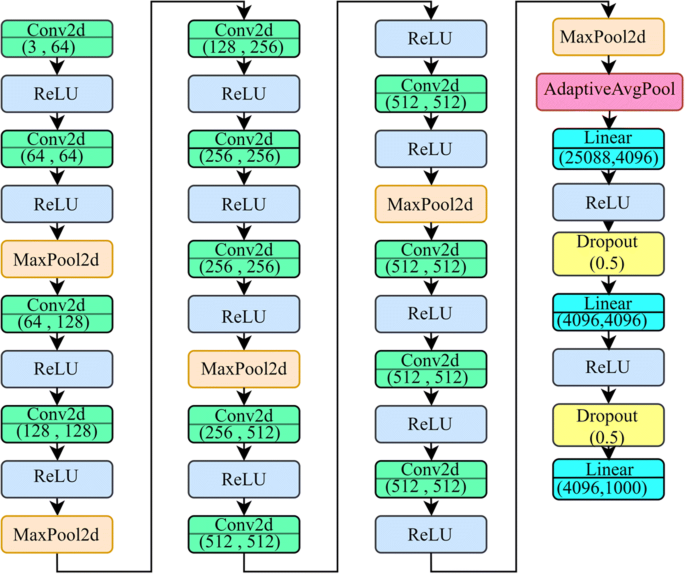
Model Architecture of VGG16
-
2.
ResNet18 - ResNet18 is known for its speed while training without any trade-off with the performance. The pre-trained model consists of a 7 × 7 convolutional layer, two pool layers, five residual blocks consisting of 3 × 3 convolutional layers. The batch normalization layer is connected with a ReLU activation function finally a fully connected layer (as shown in Fig. 4). The architecture is known for its shallowness. Also, the first two convolutional layers are neglectable. The inputs can be passed straight away to the last ReLU activation function. This model is better for classification tasks like we are conducting in this paper because of the residual block that is a bottleneck in nature, batch normalization that standardizes the outputs of subsequent layers, and the connectivity with identity to prevent the problem vanishing point gradient [13, 26].
Fig. 4 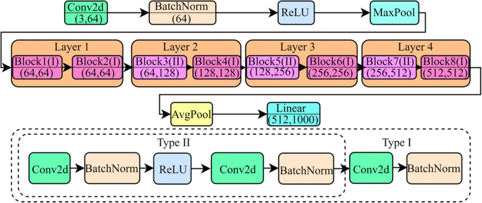
Model Architecture of ResNet18
-
3.
MobileNetV2 - as introduced by Sandler et al. [40], this network also has worked upon the reduced number of parameters for the training process and thus useful for the machines with the lower capability to handle high computational tasks. This is done with inverted residuals and inverted bottlenecks to minimize the network’s storage expenses when at work [28]. This architecture is an improvisation on its previous version, MobileNetV1. Now it has 54 layers. It takes the input of size 224 × 224. The major feature of this network is that it utilizes the depthwise separable convolutions. These type of convolutions performs two 1-dimension convolutions with the help of two kernels. This lower memory consumption is achieved since training parameters get minimized (as shown in Fig. 5). The first kind of blocks is the residual ones with one stride and the next type with stride two to lower the layers’ outputs for further computations. Each kind of block consists of 1 × 1 convolution in addition to the ReLU activation function, while the further layer being the depthwise convolution, and lastly, a 1 × 1 convolution with no linear property involved [4].
Fig. 5 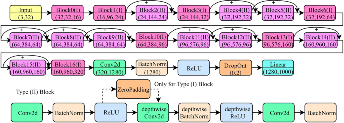
Model Architecture of MobileNetV2
-
4.
AlexNet - this CNN network was a very crucial one in the deep learning field. It consisted of different convolutions of 11 × 11, 5 × 5, 3 × 3. To downscale, the parameters max-pooling was used. Regularization is done most of the time, but instead, dropout was used to minimize overfitting. This was done on the trade-off with the training time. Out of all activation functions, ReLU was used to introduce non-linear properties in the model [23].


Figure 6 presents the pipelined block diagram of the adopted methodology further outlined in Algorithm 1.

Pipelined block diagram of the adopted methodology

4 Experimentations and results
In this section, we are going to discuss the results that were obtained when we trained the deep learning models, namely VGG16 [42], MobileNetV2 [40], ResNet18 [13], and AlexNet [23]. A multi-class classification task was performed on the dataset acquired. The classes were namely Normal, Viral Pneumonia, and COVID19. Following metrics have been used for result evaluation:
The models were evaluated on precision, recall, F1-Score, and a final accuracy of testing and training was generated and tabulated for every model in Table 3. The confusion matrix of training and testing were also plotted in Figs. 7 and 8 (MobileNetV2), Figs. 9 and 10 (VGG-16), and Fig. 11 (ResNet-18).

Training Dataset (left) and Testing Dataset (right) confusion matrix for 3 class classification using MobileNetV2

The plot of accuracy and loss overtraining and testing sets for MobileNetV2

Training Dataset (left) and Testing Dataset (right) confusion matrix for 3 class classification using VGG16

The plot of accuracy and loss overtraining and testing sets for VGG16

Training Dataset (left) and Testing Dataset (right) confusion matrix for 3 class classification using ResNet18
A model is said to be a good fit if it can generalize and learn the features from the training data without over-fitting or under-fitting, i.e., it can generalize the features and perform well even on unseen data [10, 12, 24, 25, 44]. As shown in Figs. 8, 10, and 12, the models, namely MobileNetV2, VGG-16, and ResNet-18, respectively, are unable to generalize the features. Hence even if they perform well on training data with accuracy nearing 1, they cannot give similar results on unseen data as can be seen from the fluctuation in the graph for validation accuracy curve.

The plot of accuracy and loss overtraining and testing sets for ResNet18
-
(a)
MobileNetV2
-
(b)
VGG16
-
(c)
ResNet18
-
(d)
AlexNet
The presented work adopts the AlexNet model (results depicted in Figs. 13 and 14) can outperform the above-stated models and generalize the results giving an average accuracy score of 0.98.

Training Dataset (left) and Testing Dataset (right) confusion matrix for 3 class classification using AlexNet

The plot of accuracy and loss overtraining and testing sets for AlexNet
The evaluation of results achieved by various DNNs are presented in Table 2 for each model training set and testing set belonging to all three classes.
Figure 15 shows the graphical depiction of comparisons between various DNNs on the evaluated metrics- precision, recall, and F1-score.

Comparing various DNNs on the evaluated metrics
Table 3 shows the comparative results of the presented work with other existing methods. In this study, the presented model- AlexNet outperforms existing DNNs- VGG16, ResNet18 over the selected dataset.
5 Conclusion
“Severe Acute Respiratory Syndrome CoronaVirus-2” (SARS-CoV-2), commonly referred to as novel COVID-19 (being expeditious), has been difficult to track down due to a shortage of testing kits for conducting. “Reverse Transcription - Polymerase Chain Reaction” (RT-PCR). It was the only standard assessment to acknowledge the toxin’s presence. But the time taken by this test was more than 24 hours (several days in the worst case); the primary reason behind this was testing facilities. They were compelled to conduct the exercise for large batches of samples simultaneously to cut down the cost of reagents used in chemical analysis.
Therefore, there was a need to identify a technique that can detect the infection in much less time than the existing traditional approaches. COVID-19, being a respiratory syndrome, has lungs as its preliminary target, that needs novel methods of investigation towards identifying the spread of the virus among masses. COVID19 is diverse and heterogeneous in nature, due to which our existing models and “Computer-Aided Design” (CAD) systems need to revamp in specific directions, required solely for a pandemic situation. The improved results can be collectively used in comprehending much smarter analysis by using deep learning techniques over the existing CAD systems.
Thus, this paper presents a study which has a promising future scope. It can be designed into an efficient architecture by deploying an ensemble approach with different pre-trained models that render improved accuracy over the existing ones. One of the limitations concerning this study is the lack of an extensive dataset resulting in insufficient training. Hence, we also put forward this idea that the datasets for such research-oriented problems can be maintained at a common authenticated storage space. This will further enhance the research in the contemporary research areas. The work done in this paper shows the performances of the four deep CNN, namely MobileNetV2, ResNet18, VGG16, AlexNet. VGG16 used in existing works resulted in training accuracy of 91% [6], 95.8% [20], 94.5% [14], and testing accuracy of 90.9% [20], as compared to our methodology wherein we achieved training accuracy of 97.76% And testing accuracy of 96.66%.
Similarly, MobileNetV2 used in existing works resulted in an accuracy of 96.78% [2] compared to our methodology, wherein we achieved an accuracy of 96.66%. ResNet18 showed an accuracy of 96.02% in training and 88.88% in testing. But the model which outcasted all the models mentioned above was AlexNet, which resulted in training accuracy of 97.3% and Testing Accuracy of 97.76%. Our research was based on pre-trained deep learning models, which still did not perform accurately, such that it would result in 100% accuracy.
References
Abbas A, Abdelsamea MM, Gaber MM (2021) Classification of COVID-19 in chest X-ray images using DeTraC deep convolutional neural network. Appl Intell 51(2):854–864
Apostolopoulos ID, Mpesiana TA (2020) Covid-19: automatic detection from x-ray images utilizing transfer learning with convolutional neural networks. Australas Phys Eng Sci Med 1:635–640
Ardakani AA, Kanafi AR, Acharya UR, Khadem N, Mohammadi A (2020) Application of deep learning technique to manage COVID-19 in routine clinical practice using CT images: results of 10 convolutional neural networks. Comput Biol Med 121:103795
Asnaoui KE, Chawki Y, Idri A (2020) Automated methods for detection and classification pneumonia based on x-ray images using deep learning. In Artificial intelligence and blockchain for future cybersecurity applications (pp. 257–284). Springer, Cham
Chaudhary A, Gupta V, Jain N, Santosh KC (2021) COVID-19 on Air Quality Index (AQI): A necessary evil?. In: Santosh, K., Joshi, A. (eds) COVID-19: prediction, decision-making, and its impacts. Lecture notes on data engineering and communications technologies, vol 60. Springer, Singapore. https://doi.org/10.1007/978-981-15-9682-7_14
Dansana D, Kumar R, Bhattacharjee A, Hemanth DJ, Gupta D, Khanna A, Castillo O (2020) Early diagnosis of COVID-19-affected patients based on X-ray and computed tomography images using deep learning algorithm. Soft computing, 1–9. Advance online publication. https://doi.org/10.1007/s00500-020-05275-y
Duran-Lopez L, Dominguez-Morales JP, Corral-Jaime J, Vicente-Diaz S, Linares-Barranco A (2020) COVID-XNet: a custom deep learning system to diagnose and locate COVID-19 in chest X-ray images. Appl Sci 10(16):5683
Elasnaoui K, Chawki Y (2020) Using X-ray images and deep learning for automated detection of coronavirus disease. J Biomol Struct Dyn 39(10):3615–3626. https://doi.org/10.1080/07391102.2020.1767212
Elfiky AA, Azzam EB (2020) Novel guanosine derivatives against MERS CoV polymerase: an in silico perspective. J Biomol Struct Dyn 39(8):2923–2931. https://doi.org/10.1080/07391102.2020.1758789
Fouladi S, Ebadi MJ, Safaei AA, Bajuri MY, Ahmadian A (2021) Efficient deep neural networks for classification of COVID-19 based on CT images: virtualization via software defined radio. Comput Commun 176:234–248
Ghorui N, Ghosh A, Mondal SP, Bajuri MY, Ahmadian A, Salahshour S, Ferrara M (2021) Identification of dominant risk factor involved in spread of COVID-19 using hesitant fuzzy MCDM methodology. Results Phys 21:103811
Gupta V, Jain N, Katariya P, Kumar A, Mohan S, Ahmadian A, Ferrara M (2021) An emotion care model using multimodal textual analysis on COVID-19. Chaos, Solitons Fractals 144:110708
He K, Zhang X, Ren S, Sun J (2016) Deep residual learning for image recognition. In: Proceedings of the IEEE conference on computer vision and pattern recognition (pp. 770-778)
Heidari M, Mirniaharikandehei S, Khuzani AZ, Danala G, Qiu Y, Zheng B (2020) Improving the performance of CNN to predict the likelihood of COVID-19 using chest X-ray images with preprocessing algorithms. Int J Med Inform 144:104284
Hemdan EED, Shouman MA, Karar ME (2020) Covidx-net: a framework of deep learning classifiers to diagnose covid-19 in x-ray images. arXiv preprint arXiv:2003.11055
Jain R, Jain N, Kapania S, Son LH (2018) Degree approximation-based fuzzy partitioning algorithm and applications in wheat production prediction. Symmetry 10(12):768
Jain R, Jain N, Aggarwal A, Hemanth DJ (2019) Convolutional neural network based Alzheimer's disease classification from magnetic resonance brain images. Cogn Syst Res 57:147–159
Jain N, Chauhan A, Tripathi P, Moosa SB, Aggarwal P, Oznacar B (2020) Cell image analysis for malaria detection using deep convolutional network. Intell Decis Technol 14:55–65.
Jain N, Jhunthra S, Garg H, Gupta V, Mohan S, Ahmadian A, Salahshour S, Ferrara M (2021) Prediction modelling of COVID using machine learning methods from B-cell dataset. Results Phys 21:103813
Jaiswal A, Gianchandani N, Singh D, Kumar V, Kaur M (2020) Classification of the COVID-19 infected patients using DenseNet201 based deep transfer learning. J Biomol Struct Dyn 39(15):5682–5689. https://doi.org/10.1080/07391102.2020.1788642
Khan AI, Shah JL, Bhat MM (2020) Coronet: a deep neural network for detection and diagnosis of COVID-19 from chest x-ray images. Comput Methods Prog Biomed 196:105581
Ko H, Chung H, Kang WS, Park C, Kim DW, Kim SE, Chung CR, Ko RE, Lee H, Seo JH, Choi TY, Jaimes R, Kim KW, Lee J (2020) An artificial intelligence model to predict the mortality of COVID-19 patients at hospital admission time using routine blood samples: development and validation of an ensemble model. J Med Internet Res 22(12):e25442. https://doi.org/10.2196/25442.
Krizhevsky A, Sutskever I, Hinton GE (2017) Imagenet classification with deep convolutional neural networks. Commun ACM 60(6):84–90
Kundu R, Basak H, Singh PK, Ahmadian A, Ferrara M, Sarkar R (2021) Fuzzy rank-based fusion of CNN models using Gompertz function for screening COVID-19 CT-scans. Sci Rep 11(1):1–12
Kundu R, Singh PK, Ferrara M, Ahmadian A, Sarkar R (2022) ET-NET: an ensemble of transfer learning models for prediction of COVID-19 infection through chest CT-scan images. Multimed Tools Appl 81(1):31–50. https://doi.org/10.1007/s11042-021-11319-8
Misra S, Jeon S, Lee S, Managuli R, Jang I-S, Kim C (2020) Multi-Channel transfer learning of chest X-ray images for screening of COVID-19. Electronics 9(9):1388
Narayan Das N, Kumar N, Kaur M, Kumar V, Singh D (2020) Automated deep transfer learning-based approach for detection of COVID-19 infection in chest X-rays. Ing Rech Biomed 43(2):114–119. https://doi.org/10.1016/j.irbm.2020.07.001
Narin A, Kaya C, Pamuk Z (2020) Automatic detection of coronavirus disease (covid-19) using x-ray images and deep convolutional neural networks. Pattern Analysis and Applications 24(3):1207–1220
Narin A, Kaya C, Pamuk Z (2021) Automatic detection of coronavirus disease (covid-19) using x-ray images and deep convolutional neural networks. Pattern Anal Applic 24:1–14
Ozturk T, Talo M, Yildirim EA, Baloglu UB, Yildirim O, Acharya UR (2020) Automated detection of COVID-19 cases using deep neural networks with X-ray images. Comput Biol Med 121:103792
Pan SJ, Yang Q (2009) A survey on transfer learning. IEEE Trans Knowl Data Eng 22(10):1345–1359
Panwar H, Gupta PK, Siddiqui MK, Morales-Menendez R, Singh V (2020) Application of deep learning for fast detection of COVID-19 in X-rays using nCOVnet. Chaos, Solitons Fractals 138:109944
Piryani R, Gupta V, Singh VK, Pinto D (2018) Book impact assessment: a quantitative and text-based exploratory analysis. J Intell Fuzzy Syst 34(5):3101–3110
Piryani R, Gupta V, Singh VK (2018) Generating aspect-based extractive opinion summary: drawing inferences from social media texts. Computación y Sistemas 22(1):83–91
Polsinelli M, Cinque L, Placidi G (2020) A light CNN for detecting COVID-19 from CT scans of the chest. Pattern recognition letters, 140:95–100. https://doi.org/10.1016/j.patrec.2020.10.001
Raza A, Ahmadian A, Rafiq M, Salahshour S, Ferrara M (2020) An analysis of a non-linear susceptible-exposed-infected-quarantine-recovered pandemic model of a novel coronavirus with delay effect. Results Phys 21:103771
Razzaq OA, Rehman DU, Khan NA, Ahmadian A, Ferrara M (2021) Optimal surveillance mitigation of COVID'19 disease outbreak: fractional order optimal control of compartment model. Results Phys 20:103715
Rowan NJ, Laffey JG (2020) Challenges and solutions for addressing critical shortage of supply chain for personal and protective equipment (PPE) arising from coronavirus disease (COVID19) pandemic–case study from the Republic of Ireland. Sci Total Environ 25:138532
Salman FM, Abu-Naser SS, Alajrami E, Abu-Nasser BS, Alashqar BA (2020) Covid-19 detection using artificial intelligence
Sandler M, Howard A, Zhu M, Zhmoginov A, Chen LC (2018) Mobilenetv2: inverted residuals and linear bottlenecks. In: Proceedings of the IEEE conference on computer vision and pattern recognition (pp. 4510-4520)
Shariq M, Singh K, Bajuri MY, Pantelous AA, Ahmadian A, Salimi M (2021) A secure and reliable RFID authentication protocol using Schnorr digital cryptosystem for IoT-enabled healthcare in COVID-19 scenario. Sustain Cities Soc 75:103354
Simonyan K, Zisserman A (2014) Very deep convolutional networks for large-scale image recognition. arXiv preprint arXiv:1409.1556
Singh D, Kumar V, Kaur M (2020) Classification of COVID-19 patients from chest CT images using multi-objective differential evolution–based convolutional neural networks. Eur J Clin Microbiol Infect Dis 39(7):1379–1389. https://doi.org/10.1007/s10096-020-03901-z
Singh PK, Saha P, Mukherjee D, Ahmadian A, Ferrara M, Sarkar R (2021) GraphCovidNet: a graph neural network based model for detecting COVID-19 from CT scans and X-rays of chest. Sci Rep 11(1):1–16
Yamashita R, Nishio M, Do RKG, Togashi K (2018) Convolutional neural networks: an overview and application in radiology. Insights Into Imaging 9(4):611–629
Zamir M, Shah K, Nadeem F, Bajuri MY, Ahmadian A, Salahshour S, Ferrara M (2021) Threshold conditions for global stability of disease free state of COVID-19. Results Phys 21:103784
Author information
Authors and Affiliations
Contributions
The authors have contributed equally in this research work.
Corresponding author
Ethics declarations
Ethical approval
This article does not contain any studies with human participants or animals performed by any of the authors. Informed consent was obtained from all individual participants included in the study.
Conflict of interest
The authors declare that they have no competing interests.
Informed consent
Not applicable.
Additional information
Publisher’s note
Springer Nature remains neutral with regard to jurisdictional claims in published maps and institutional affiliations.
Rights and permissions
Springer Nature or its licensor holds exclusive rights to this article under a publishing agreement with the author(s) or other rightsholder(s); author self-archiving of the accepted manuscript version of this article is solely governed by the terms of such publishing agreement and applicable law.
About this article

Cite this article
Gupta, V., Jain, N., Sachdeva, J. et al. Improved COVID-19 detection with chest x-ray images using deep learning. Multimed Tools Appl 81, 37657–37680 (2022). https://doi.org/10.1007/s11042-022-13509-4
Received:
Revised:
Accepted:
Published:
Issue Date:
DOI: https://doi.org/10.1007/s11042-022-13509-4