Abstract
“There’s Plenty of Room at the Bottom”, said the title of Richard Feynman’s 1959 seminal conference at the California Institute of Technology. Fifty years on, nanotechnologies have led computer scientists to pay close attention to the links between physical reality and information processing. Not all the physical requirements of optimal computation are captured by traditional models—one still largely missing is reversibility. The dynamic laws of physics are reversible at microphysical level, distinct initial states of a system leading to distinct final states. On the other hand, as von Neumann already conjectured, irreversible information processing is expensive: to erase a single bit of information costs ~3 × 10⁻²¹ joules at room temperature. Information entropy is a thermodynamic cost, to be paid in non-computational energy dissipation. This paper addresses the problem drawing on Edward Fredkin’s Finite Nature hypothesis: the ultimate nature of the universe is discrete and finite, satisfying the axioms of classical, atomistic mereology. The chosen model is a cellular automaton (CA) with reversible dynamics, capable of retaining memory of the information present at the beginning of the universe. Such a CA can implement the Boolean logical operations and the other building bricks of computation: it can develop and host all-purpose computers. The model is a candidate for the realization of computational systems, capable of exploiting the resources of the physical world in an efficient way, for they can host logical circuits with negligible internal energy dissipation.
1 Cellular Automata and the Physics of Information
Cellular Automata (CA) are mathematical representations of complex dynamical systems whose macro-behaviour is determined by non-linear relations among its micro-constituents. Several features make CA appealing to information scientists. Firstly, they simulate a variety of adaptive processes: from urban evolution (Batty 2005), to Ising models (Creutz 1986), neural networks (Franceschetti et al. 1992), and turbulence phenomena (Chen et al. 1983). Secondly, they are useful toy universes for the study of pattern formation: complexity emerges from the elementary entities performing almost trivial computations; yet, simple computations lead to complex and unpredictable behaviour (Crutchfield and Mitchell 1995).
There is a third reason to study CA—the one we are dealing with in this paper. Physicists and philosophers have argued at length for and against a discrete nature of the fundamental layer of reality.Footnote 1 We will take the discrete side as a working hypothesis, being interested in exploring how CA may be used to ground an ontology of the physical world that is both computationally tractable and philosophically transparent. Whether or not our own universe is indeed a discrete CA implementing the rule we expose below, we are interested in the tenability of such a universe and the fruitfulness of its structure for further CA-based enquiries.Footnote 2
The best way to introduce a digital universe is by analogy with a physical system we are intimately acquainted to: our universe is to be conceived as a computer, whose characteristic activity, at each instant of time t, consists in computing its overall state at t + 1: “information plays as a primordial variable shaping the course of development of the universe” (Ilachinski 2001): 605), together with space and time. Two distinctive features of CA are discreteness and determinism. The model to be exposed below adds a third constraint: finiteness. There is no place for actual infinity in our theory. The framework is a proper implementation of what computational physicist Edward Fredkin has called Finite Nature hypothesis:
Finite Nature is a hypothesis that ultimately every quantity of physics, including space and time, will turn out to be discrete and finite; that the amount of information in any small volume of space–time will be finite and equal to one of a small number of possibilities. […] Finite Nature implies that the basic substrate of physics operates in a manner similar to the workings of certain specialized computers called cellular automata (Fredkin 1993: 117).
2 A Digital Universe
Let us start by illustrating some features common to all CA, and the specific choices made for our universe (call it U):
-
1.
Discrete space–time A CA consists of a lattice of cells. The lattice can be n-dimensional, but most of the models in the literature use one or two dimensions. Our U is two-dimensional, allowing us both (a) to model certain physical phenomena and (b) to retain the intuitive appeal of a simple mereotopological structure. A cell is taken as a mereotopological atom: a simple that cannot be further decomposed into smaller parts. Since U must be finite and discrete to comply with the aforementioned constraints, spacetime is finite and discrete: there is some finite number N, however large, so that exactly N cells exist in U. We assume that time is also discrete, and divided into minimal units t 0, t 1,….
-
2.
Homogeneity All cells are morphologically identical. In two dimensions, only three regular polygons can uniformly divide space, preserving the rotational and translational symmetries for each point of the lattice: equilateral triangle, square, and hexagon. While most scientists studying CA choose the square (e.g., Conway’s famous Game of Life), in our lab we have opted for the hexagon. Our grid looks thus:
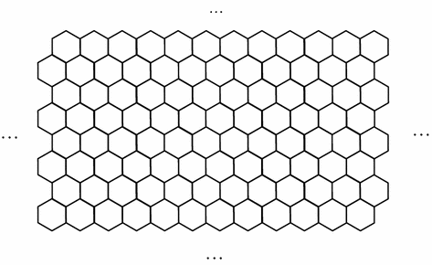

The hexagonal lattice was preferred for its topological virtues. However, the results achieved by our computer simulations, to be exposed below, can be replicated in a square-based structure thanks to the rule governing the behaviour of the entire universe, as explained in the next section. Once a system of coordinates has been defined, a cell can be identified with an ordered pair of integers <i, j> representing its place in the grid.
-
3.
Discrete states At any instant t, any cell <i, j> instantiates one state σ ∈ Σ, where Σ is a finite set of cardinality ∣Σ∣ = k. “σ i, j, t ” shall denote the state of cell <i, j> at time t.
-
4.
Local interactions Any cell <i, j> interacts only with its immediate neighbourhood, represented by the six cells surrounding <i, j>. Let us conventionally number them counter-clockwise:
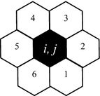
… And let us have “[i, j]” denote the neighbourhood of <i, j>.
-
5.
Rules At any instant, each <i, j> updates its state by implementing a mapping ϕ from states to states, <i, j>’s state at t + 1 being determined by the states of [i, j] at t:
$$\upsigma_{i,j,t + 1} =\upphi(\upsigma_{{\left[ {i, \, j} \right],t}} )$$

Ontologically, our universe is homogenous in two senses: (a) from the mereotopological point of view, any cell is morphologically identical to any other; and (b) all cells are governed by the same rule.Footnote 3 Moreover, our universe is synchronous: all points in space–time update their state simultaneously. This is by far the most popular option in the field (compare Ingerson and Buvel 1984). U has, thus, three features in common with virtually every other CA:
-
1.
Information is (locally) finite Any lesser part of reality embeds a finite quantity of information, and the same is true for the whole U. Let us call a configuration of U at t the global state of U at instant t. This can be represented by a vector: the configuration of U at t, \({\overline{\upsigma }}_{t}\), is just the ordered sequence of the states of every cell at t: \({\overline{\upsigma }}_{t}\) = <σ0, 0, t, σ0, 1, t, σ1, 0, t, σ1, 1, t, σ1, 2, t, …, σ i, j, t, …, σ m, n, t > ∈ Γ, where Γ is the phase space or set of global configurations.
Since any cell can be in one of a finite number of states∣Σ∣ = k, and there is a finite number N of cells, there will be k N possible configurations. The entire evolution of U is a finite transition graph, G Φ, the graph of the global rule Φ: Γ → Γ induced by ϕ, mapping configurations to configurations:
$${\overline{\upsigma }}_{t + 1} = \varPhi ({\overline{\upsigma }}_{t} )$$As G Φ is finite, no matter what the starting configuration is, the universe will exhibit periodic behaviour after k N iterations of Φ.
-
2.
Information is processed locally If there are so-called actions at a distance (as per the famous Einstein et al. 1935 thought experiment), these should be taken as emergent: any point in the lattice has its state at time t completely determined by what happened in its neighbourhood at t − 1.
-
3.
Information is processed in parallel fashion by the cells.
Our model shares features (1)–(3) with many other CA. However, U also has a fourth one that makes it different from most CA in the literature, including Conway’s Life:
-
4.
Information is preserved This is achieved via a somewhat uncommon rule, one that allows our model to be time-reversal invariant. To explain this, in the following paragraphs
-
(a)
We first define what it is for a rule to be reversible, and distinguish between two levels of reversibility—a weak one and a strong one (§ 3);
-
(b)
We the define our ϕ (§ 4);
-
(c)
We show that ϕ is strongly reversible, and explain the implications for the computational efficiency of the model (§ 5).Footnote 4
-
(a)
3 Weak and Strong Reversibility
A local CA rule ρ is called irreversible when different inputs can generate the same output. Likewise, a global rule P is irreversible when different global configurations at t − 1 can generate the same configuration at t. This entails that it is not generally possible to look at a CA configuration at t and determine what its configuration was the instant before.
A rule ρ: A → B is (weakly) reversible when it has an inverse ρ−1: B → A, with ρ−1 ○ ρ = Id A: A → A and ρ ○ ρ−1 = Id B: B → B, Id being the identity function, (ρ−1 ○ ρ) (σ i, j, t ) = ρ−1 (ρ (σ i, j, t )) = σ i, j, t . The same goes for the global Ρ: Γ → Γ. If Ρ is reversible, each \({\overline{\upsigma }}\) ∈ Γ has exactly one preceding configuration \({\overline{\upsigma }}_{1}\) ∈ Γ, such that P(\({\overline{\upsigma }}_{1}\)) = \({\overline{\upsigma }}\). Once the inverse of a reversible rule is on the table, we can run a CA backwards, going through its past configurations.
A rule ρ is strongly reversible (or time-reversal invariant) when it is the inverse of itself, ρ−1 = ρ. Strong reversibility entails weak reversibility. If ρ is strongly reversible, the history of the universe can be recovered by running the same rule backwards, via a mapping inverting time: t |→ −t.
4 Rule
Most CA have irreversible rules: the set of states in [i, j] at t − 1 cannot in general be discovered just by looking at the state of <i, j> at t. Thus, a local rule generating a time-reversal invariant CA requires careful definition. We start by assuming that any cell state is represented, not by a single bit, but by a sextuple of bits, one for each side of the cell. Any bit can be 1 (on, active) or 0 (off, inactive). The state <i, j> at t is therefore σ i, j, t = <x 1, x 2, x 3, x 4, x 5, x 6>, where x 1 represents side 1, x 2 side 2, etc., and each x has a value v ∈ V = {0, 1}. Each cell has 26 possible states.
The neighbourhood [i, j] works in a somewhat unorthodox way: while retaining the general form of any CA rule, σ
i, j, t+1 = ϕ(σ[i, j], t
), we stipulate that only the value v ∈ V of the neighbouring side is relevant for computation. We number these sides counter-clockwise, too. Our rule is therefore a ϕ: {0, 1}6 → {0, 1}6. To help intuition, imagine the dynamics thus: each cell reads or perceives the output of the neighbouring sides of the six cells nearby, thinks about it by computing the output applying ϕ, and acts by exhibiting the output to its neighbourhood:
Now the rule goes thus:
… ∑
v[i, j],
t
(mod 2) being the sum modulo 2 of the v ∈ {1, 0} in the input sextuple at t. Id is identity on Σ, mapping every σ ∈ Σ onto itself: Id(<x
1, x
2, x
3, x
4, x
5, x
6>) = <x
1, x
2, x
3, x
4, x
5, x
6>:
Perm: Σ → Σ is a permutation on Σ, a function that, for every sextuple, exchanges the first three bits with the other three and vice versa, Perm(<x
1, x
2, x
3, x
4, x
5, x
6>) = <x
4, x
5, x
6, x
1, x
2, x
3>:
Now (a) if the number of on-bits in the input for any cell <i, j> is odd (sum modulo 2 = 1), atom <i, j> triggers Perm. The information arriving from a neighbouring cell will be then be transmitted to the opposite site. For a simple example illustrating the dynamics, let us paint a side in black when v = 1. Here is a single bit, perceived by <i, j> in the neighbouring cell <g, h> at t:
This is just aid to “topological imagination”. Computationally, <i, j> receives a specific sextuple from [i, j]: “single 1 coming from upper left” means [i, j] = <0, 0, 0, 1, 0, 0> (or, for brevity, 000100). Given the input, <i, j> computes Perm(000100) = 100000. At t + 1 our cell displays to the neighbouring cells the following configuration:
Suppose now that <k, l> is in the same state as <i, j> was one instant before, having as its only on-bit in its [k, l] the one exposed at t + 1 by <i, j>: [k, l] = 000100. Now <k, l> triggers Perm too, so that at t + 2 we get:
The effect is uniform rectilinear movement of the active bit from top left to bottom right (all local movements in our U are apparent, being the phenomenal result of cells turning on and off their bits):
The same happens in each case of input with an odd number of active bits. Here are three of them converging on <i, j> from directions 2, 3 and 4:
(b) When the sum of the values in the sextuples is even (so Id is triggered), signals are bounced back where they came from. Here are two active bits converging on <i, j> from directions 2 and 4:
5 Niceties
The rule is a simple conditional routing of signals: when the sum modulo 2 of input members is 0, it’s rectilinear uniform movement; when the sum is 1, it’s signal kickback. Now:
-
1.
The rule guarantees a conservation of the total number of active and inactive bits since the beginning of the universe. Since Perm and (trivially) Id are permutations, whatever the input sextuple is, the output sextuple has the same amount of ones and zeros.
-
2.
Besides being conservative, the rule is reversible: each input is mapped both by Id and by Perm to a distinct output.
-
3.
The rule coincides with inverse, to which it is mapped by the time-reversing transformation: t |→ −t. Obviously, Id is strongly reversible. But Perm is, too: given any input <a, b, c, d, e, f> not only is it mapped to a distinct output <d, e, f, a, b, c>; but also, the rule to move back from output <d, e, f, a, b, c> to its (unique) input still is Perm(<d, e, f, a, b, c>) = <a, b, c, d, e, f>.
That the ϕ is strongly reversible entails that the corresponding global graph, G, hosts no so-called garden-of-eden, i.e., no configuration can appear only as the initial setting of U, not being producible by the evolution of the universe. Moore and Myhill’s combined (Myhill 1963) results show that garden-of-eden configurations exist iff there exist configurations with more than one predecessor, which is ruled out by reversibility.
6 Information Entropy
Irreversible dynamics entail information entropy: the application of an irreversible rule ρ in a CA can erase an amount of information concerning the immediate past of the universe. An AND gives 0 as its output at t. What was the input at t − 1? 1 and 0, or vice versa, or two zeros? We may never know, by looking at the universe at t. Until the seventies, however, researchers were not very interested in reversible CA, for such CA were deemed unable of supporting universal computation, that is, of evaluating any computable function, as a universal Turing machine (UTM) does. However, in (1973) Charles Bennett proved that universal computation doesn’t necessarily require irreversible logical gates, and in (1977) Toffoli produced the first reversible CA capable of emulating a UTM.
There are (at least) two reasons of dissatisfaction with irreversible computation, one technical, one theoretical. The technical point is that irreversible computation has a regrettable energetic cost: as conjectured in von Neumann (1966) and strengthened and justified in Landauer (1961), to erase a bit of information costs ~3 × 10⁻²¹ joules at room temperature. Informational entropy has a thermodynamic cost, to be paid in with the coin of non-computational energy dissipation. This is not due to inefficient circuit design: it is directly entailed by the presence of irreversible logical operations. As nanotechnology advances, this energy dissipation problem is going to put more and more pressure on irreversible architectures.Footnote 5
The theoretical reason of dissatisfaction with irreversible computational models is that they can only mirror macroscopic physical reality, never reaching the bottom of what is out there. The dynamical laws of physics are reversible at the micro-level: distinct initial states in the evolution of a microphysical system always lead to distinct final states. So it seems that, if one wants a CA to capture what is really going on out there at the basic ontological level, one had better resort only to reversible rules (which also secure the preservation of the relevant additive quantities), on pain of having to abandon the intuition of a basic isomorphism between physics and information.
7 Universal Computation
ϕ allows our CA to emulate universal Turing machines capable of computing (assuming Turing’s Thesis) anything computable. A CA rule capable of this is called computation universal. There are two main ways to prove that a CA rule is computation universal in the literature. One consists in reducing the rule to another one, of which it is already known that it is computation universal. The other, more constructive, method is based on directly showing that all the basic building bricks of computation can be emulated by patterns generated by the CA rule. This is the strategy adopted, e.g., in the celebrated original proof by Berkelamp et al. (1982) that Conway’s Life is computation universal, and shall also be followed by us with respect to ϕ.
In order for a CA to be computation universal, it has to be capable of producing stable patterns of state configurations: structured packages of information that can move across the lattice. More precisely, the primitives of computation consist in the (1) transmission and (2) storage of signals, which call for a system memory and wires (along which information bits can move, be stored in periodic rings, sent in different directions, copied, etc.), and (3) the logical processing of signals, requiring a functionally complete set of gates, such as AND, OR and NOT. Once one has shown that a CA can host these building bricks, the factual design of circuits corresponding to some computing system or other is academic.
As Fredkin and Toffoli have shown in their classic Conservative Logic, points (1) and (2) above are conceptually realized by a single primitive in a reversible CA: “there is no intrinsic distinction between signal conservation and transmission” (Fredkin and Toffoli 1982: 224; see also Margolus 1984). For instance, take a signal s connecting two space–time locations, L1 and L2. If L1 and L2 are spatially separated, then we shall claim that s has been passed on from one to the other in a given time interval. But if L1 and L2 are co-localized, we shall say that s has been stored in the (unique) location L1 ≡ L2 across distinct times—compare Fredkin and Toffoli’s (1982) intuitive example: s is a message sent to my secretary via e-mail (transmission); s is written on a post-it I leave on my desk for the secretary to read the day after (storage): one physical process, described in two fashions.
In the model each cell performs the two tasks of signal storage and signal transmission, insofar as it implements rule ϕ. We know that an odd number of active input bits triggers Perm, having the signal transmitted to the cell neighbourhood with uniform rectilinear movement. Each atom, thus, works as a circuit-unit, the role of a circuit-unit consisting in moving bits from the point in the lattice it consists into the next one:
We can have circuits of arbitrary length taken as successions of circuit-units. A rectilinear circuit of length n is a route of adjacent cells a given signal, such as a sequence of bits, can follow, and whose extremes are also separated by n time units or instants, given that the signal moves at the speed of exactly one cell per time unit. Besides, it is easy to implement a finite size memory by means of coded sequences of bits, moving in circles or forming periodic or stable configurations via suitable deviations and kickbacks (we will see a couple of examples infra). But there is also a more pregnant sense in which U has memory of anything going on in it: since its dynamic rule is time-reversal invariant, the universe retains perfect memory of its initial configuration \({\overline{\upsigma }}_{0}\) during all of its evolution, given that no information bit is erased, and that any past configuration can be recovered thanks to reversibility.
The tricky part consists in showing that U can process its information on the basis of a functionally complete set of logical gates. In any reversible CA, computation has to be a conditional routing of signals: these have to be taken as unalterable objects that can be moved here and there, but never created or destroyed. Now a Boolean logic based on AND, NOT and the duplication of signals is functionally complete. However, the ordinary AND is irreversible; and intuitively a signal duplication seems to entail a creatio ex nihilo of information incompatible with the conservative requirement.
However, these issues are solved in the model. Each <i, j> in the universe is a universal logical gate because it is a locus for the transition (linear transmission or clash-and-kickback) of information bits and bit sequences. To begin with, we know that a conservative gate has to have an equal number of inputs and outputs. Now, 2-input/2-output logical gates cannot do the trick. We have 44 = 256 possible truth tables for them, of which 24 are reversible. Margolus (1988) has proved that these can all be reduced to compositions out of XOR, and XOR alone is not universal.
Therefore, we need to increase the number of input and output lines. In the literature, there are universal reversible gates, such as Fredkin’s 3-input/3-output gate, but implementing them in a CA is no trivial business (the only case we are aware of is Fredkin and Toffoli’s 1982 billiard ball model; see also Toffoli and Margolus 1990). We take each cell in the grid as a gate taking inputs at t from three of its sides, providing its output on three sides at t + 1. Intuitively, this means that in the simulation of unary operations (think NOT), or binary ones (think AND), some inputs and outputs are pleonastic. Given a function f with a suitable number of inputs-outputs, we can have a function g merged in f, with a smaller number of inputs-outputs, by assigning pre-specified constant (or also periodic, but we’ll skip this case here) values to certain input lines, and by disregarding certain output lines (the so-called garbage bits). We claim, then, that f emulates g via constants and garbage.
Back to cell <i, j>. Assume it to take as input streams of signals coming from directions x, y, and z indicated in dark grey below (corresponding to directions 4, 5, and 6 in the numbering above); and to provide as output the signals on the opposite directions, in pale grey:
7.1 AND
Each cell can implement a reversible AND: take z as a “control line”, activated by fixing its value as z = 1, by a stream of active bits come from that direction. Now consider the bit streams coming from x and y as the AND inputs. The cell outputs the conjunction of x and y, both in the x- and in the y- output direction; both take value 1 iff the x-input and y-input are 1:
7.2 NOT
Next, each cell realizes NOT along the same lines: hold fixed z = 1 and y = 0. The z-output is the negation of the x-input, that is, if input x = 1, output z = 0, and if input x = 0, output z = 1:
7.3 Duplication
{AND, NOT} is functionally complete. We can have each cell realize a certain duplication of signals, too. In a reversible environment duplication has to respect precise requirements: “If we allow signals to split in the forward direction, we also have to allow two signals to ‘join’ in the reverse direction. We therefore require that all fan-outs occur only within individual signal processing elements” (Ilachinski 2001: 316).
This happens in U, where each cell can duplicate signals by means of the NOT input pattern: hold fixed z = 1 and y = 0, and the given cell <i, j> will provide two copies of the x-input, one out of the same z-input side, the other out of the same x-input size:
That a copy of x is redirected towards the same side it came from means that this configuration can be used also to realize the kickback of signals of arbitrary length.
7.4 Delays
When building logical circuits, one usually needs to introduce deviations, bounces, and delays. Simple kickbacks, as we know, are guaranteed for single bits in all cases in which an odd number of active bits converges on a cell simultaneously, triggering Id. The pattern for negation can be also used to build translations and delays of signals of any length. NOT is implemented in the cells by having it make an angle of 120°. Therefore, we can use suitably arranged couples of NOT gates, the second item in each couple negating the stream negated by the first in order to give us back the original signal, to realize angles at will. For instance, consider a simple circuit with the following shape—with the black arrow indicating the direction of a sequence of bits (say, 10110111), and the grey arrow indicating the way of the corresponding negated sequence (01001000):
The signal comes out delayed of exactly four time units with respect to the dotted rectilinear route.
8 Conclusions
By supporting the primitives of computation as instantiated by a digital computer, the ϕ-rule-based CA is capable of universal computation: if we identify the initial configuration \({\overline{\upsigma }}_{0}\) of the CA with the starting data of the universe, its evolution as prescribed by ϕ (with the corresponding induced global rule Φ) is the program by means of which the universe elaborates those data. Thanks to ϕ, the universe can produce and host all-purpose computers, implement finite algorithms and evaluate computable functions. Besides, all the operations realized by the cells are (1) conservative (2) reversible and (3) invariant.
By producing our ϕ-rule-based CA, we put forward a new CA that satisfies natural constraints from the ontology of physics and may well serve as a model to understand the duality of physical processes and information (compare it with the aforementioned, popular Game of Life which is equally simple, but not reversible). Moreover, the precise language of computation allows for a neat and transparent ontology, built with well understood primitives and a limited number of basic concepts: while conceptually simple, a universal CA is capable of complex behaviour—it’s by playing around with interesting toy universes, pretty much like a scientific observer, that we can hope to get a better grasp of the fundamental notions of our physical universe: laws, events, processes.Footnote 6
Finally, as U can host UTM’s, the universe might be unpredictable in a precise sense: given that the Halting Problem is not Turing-computable (and assuming, of course, there is no oracle solving the Halting Problem for the relevant machine: this is an open issue in science), there is no general algorithm capable of predicting whether the given UTM with a given input will halt after n steps providing its output. The same would hold for any physical universe, insofar as it is capable of universal computation and mimics the underlying ontology of U: beyond a certain pattern complexity, the only way to know what is going to happen would consist in having the software implementing the CA run, and look.
Notes
The philosophically savvy reader may have noticed the indirect reference to David Lewis’ Humean Supervenience thesis: see Lewis (1986, p. ix).
For a study of non-homogeneous CA, see Sipper (2004).
The universe can easily be seen as satisfying the axioms of classical mereology as formalized in a standard first-order logical language, in its atomistic version, once we have the individual variables of the language range on atomic cells, and aggregates thereof. Details are not essential for the results that follow, but the interested reader by consult Tagliabue (2013b) for the full formal picture and how it relates to atomicity and the finite nature of the universe.
There has been a revival of philosophical interest in the link between computation and thermodynamics cost—see for example Maroney (2005) for a challenge and Ladyman et al. (2007) for a thorough reply. In 2012 a paper published in Nature claimed to have experimentally measured the erasure principle (see Bérut et al. 2012).
References
Batty, M. (2005). Cities and complexity, understanding cities with cellular automata, agent-based models, and fractals. Cambridge, MA: MIT Press.
Bennett, C. (1973). Logical reversibility of computation. IBM Journal of Research and Development, 6, 525–532.
Berkelamp, E. R., Conway, J. H., & Guy, R. K. (1982). Winning ways for your mathematical plays. New York: Academic Press.
Berto, F., & Tagliabue, J. (2014). The world is either digital or analogue. Synthese, 191, 481–497.
Bérut, A., Arakelyan, A., Petrosyan, A., Ciliberto, S., Dillenschneider, R., & Lutz, E. (2012). Experimental verification of Landauer’s principle linking information and thermodynamics. Nature, 483(7388), 187–190.
Chen, H., Chen, S., Doolen, G., & Lee, Y. C. (1983). Simple lattice gas models for waves. Complex Systems, 2, 259–267.
Creutz, M. (1986). Deterministic Ising dynamics. Annals of Physics, 167, 62–76.
Crutchfield, J. P. (1994). The calculi of emergence: Computation, dynamics, and induction. Physica D, 75, 11–54.
Crutchfield, J. P., & Mitchell, M. (1995). The evolution of emergent computation. Proceedings of the National Academy of Sciences, 92(23), 10742.
Einstein, A., Podolski, B., & Rosen, N. (1935). Can quantum mechanical description of physical reality be considered complete? Physical Review, 37, 777.
Floridi, L. (2009). Against digital ontology. Synthese, 168(1), 151–178.
Franceschetti, D. R., Campbell, B. W., & Hamneken, J. W. (1992). Hamming nets, Ising sets, cellular automata, neural nets and random walks. American Journal of Physics, 61, 50–53.
Fredkin, E. (1993). A new cosmogony. In D. Matzke (Ed.), PhysComp92 (pp. 116–121). Los Alamitos, CA: Computer Society Press.
Fredkin, E., & Toffoli, T. (1982). Conservative logic. International Journal of Theoretical Physics, 21, 219–254.
Ilachinski, A. (2001). Cellular automata. A discrete universe. Singapore: World Scientific.
Ingerson, T. E., & Buvel, R. L. (1984). Structure in asynchronous cellular automata. Physica D, 10, 59–68.
Ladyman, J., Presnell, S., Short, A. J., & Groisman, B. (2007). The connection between logical and thermodynamic irreversibility. Studies in History and Philosophy of Science Part B: Studies in History and Philosophy of Modern Physics, 38(1), 58–79.
Landauer, R. (1961). Irreversibility and heat generation in the computing process. IBM Journal of Research and Development, 5, 183–191.
Lewis, D. (1986). Philosophical papers volume II. Oxford: Oxford University Press.
Margolus, N. (1984). Physics-like models of computation. Physica D, 10, 81–95.
Margolus, N. (1988). Physics and computation, Ph.D. Thesis, Tech. Rep. MIT.
Maroney, O. (2005). The (absence of a) relationship between thermodynamic and logical reversibility. Studies in History and Philosophy of Science Part B: Studies in History and Philosophy of Modern Physics, 36(2), 355–374.
Myhill, J. (1963). The converse of Moore’s Garden of Eden theorem. Proceedings of the American Mathematical Society, 14, 685–686.
Sipper, M. (2004). Evolution of parallel cellular machines. The cellular programming approach. New York: Springer.
Tagliabue, J. (2013a). Digital Philosophy. In H. Zenil (Ed.), Irreducibility and Computational Equivalence (pp. 325–339). Springer.
Tagliabue, J. (2013b). Digital Philosophy. Formal Ontology and Knowledge Representation in Cellular Automata. Ph.D. Dissertation, San Raffaele University.
Toffoli, T. (1977). Computation and construction universality of reversible cellular automata. Journal of Computer and System Sciences, 15, 213.
Toffoli, T., & Margolus, N. (1990). Invertible cellular automata: A review. Physica D, 45, 229–252.
Von Neumann, J. (1966). Theory of self-reproducing automata. Champaign, IL: University of Illinois Press.
Zenil, H. (Ed.). (2013a). Irreducibility and computational equivalence. New York: Springer.
Zenil, H. (Ed.). (2013b). A computable universe. Singapore: World Scientific.
Author information
Authors and Affiliations
Corresponding author
Rights and permissions
Open Access This article is distributed under the terms of the Creative Commons Attribution 4.0 International License (http://creativecommons.org/licenses/by/4.0/), which permits unrestricted use, distribution, and reproduction in any medium, provided you give appropriate credit to the original author(s) and the source, provide a link to the Creative Commons license, and indicate if changes were made.
About this article

Cite this article
Berto, F., Tagliabue, J. & Rossi, G. There’s Plenty of Boole at the Bottom: A Reversible CA Against Information Entropy. Minds & Machines 26, 341–357 (2016). https://doi.org/10.1007/s11023-016-9401-6
Received:
Accepted:
Published:
Issue Date:
DOI: https://doi.org/10.1007/s11023-016-9401-6