Learning from interpretation transition

Abstract

We propose a novel framework for learning normal logic programs from transitions of interpretations. Given a set of pairs of interpretations (I,J) such that J=T _P (I), where T _P is the immediate consequence operator, we infer the program P. The learning framework can be repeatedly applied for identifying Boolean networks from basins of attraction. Two algorithms have been implemented for this learning task, and are compared using examples from the biological literature. We also show how to incorporate background knowledge and inductive biases, then apply the framework to learning transition rules of cellular automata.

1 Introduction

There is a growing interest in learning dynamics of systems in the field of inductive logic programming (ILP) (Muggleton et al. 2012) with applications in planning, scheduling, robotics, bioinformatics, and adaptive and complex systems. In the view that a logic program is a state transition system (Inoue 2011; Inoue and Sakama 2012), given an Herbrand interpretation representing a current state of the world, a logic program P specifies how to define the next state of the world as an Herbrand interpretation through the immediate consequence operator (also called the T _P operator) (van Emden and Kowalski 1976; Apt et al. 1988). Based on this idea, we here propose a framework to learn logic programs from traces of interpretation transitions.

The learning setting is as follows. We are given a set of pairs of Herbrand interpretations (I,J) such that J=T _P (I) as positive examples, and the goal is to induce a normal logic program (NLP) P that realizes the given transition relations. As far as the authors know, this concept of learning from interpretation transition (LFIT) has never been considered in the ILP literature. In fact, LFIT is different from any method to learn Boolean functions that has been developed in the field of computational learning theory (Kearns and Vazirani 1994) in the sense that LFIT learns dynamics of systems, while the conventional learning setting is not involved in dynamics. A closer setting can be found in learning from interpretations (LFI) (De Raedt 1997), in which positive examples are given as Herbrand models of a target program, but again the goal of LFI is not to learn dynamics of systems. Learning action theories (Moyle 2003; Otero 2005; Inoue et al. 2005; Tran and Baral 2009; Corapi et al. 2011; Rodrigues et al. 2012) can also be related with LFIT, but its goal is not exactly the same as that of LFIT. In particular, LFIT can learn dynamics of systems with positive and negative feedbacks, which have not been much taken into account in the literature. Relational reinforcement learning (Džeroski et al. 2001) can consider feedbacks in the learning process as rewards, but LFIT learns how such feedbacks can be represented logically by state transition rules. Learning NLPs rather than definite programs has been considered in ILP, e.g., (Sakama 2001), but most approaches do not take the LFI setting. Moreover, from the semantical viewpoint, our framework can learn NLPs under the supported model semantics (Apt et al. 1988) rather than the stable model semantics (Gelfond and Lifschitz 1988).

An intended direct application of LFIT is learning transition or update rules in dynamical systems such as Boolean networks (Kauffman 1993) and cellular automata (Wolfram 1994), which have been respectively used as mathematical models of genetic networks and complex adaptive systems. It has been observed that the T _P operator for an NLP P precisely captures the synchronous update of the corresponding Boolean network, where each gene and its regulation function correspond to a ground atom and the set of ground rules with the atom in their heads, respectively (Inoue 2011). Then, given an input Herbrand interpretation I, which corresponds to a gene activity profile (GAP) with gene disruptions for false atoms in I and gene overexpressions for true atoms in I, the interactions between genes are experimentally analyzed by observing an output GAP J such that J=T _P (I) is assumed to hold after a time step has passed. In this setting, LFIT of an NLP P corresponds to inferring a set of gene regulation rules that are complete for those experiments of 1-step GAP transitions. Such a learning task has been analyzed in the literature (Akutsu et al. 2003, 2009), but no ILP technique has been applied to the problem. Besides, 2-state cellular automata, in which each cell can take either 1 or 0 as a possible value, are instances of Boolean networks, so that their state transitions are determined by the T _P operator (Blair et al. 1997). Hence it should be possible to apply LFIT for their learning tasks. Learning transition rules (called identification) of cellular automata has been studied in the literature (Adamatzky 1994, 2007), but again no previous work has employed ILP techniques on this problem.

It is known that any trajectory from a GAP in a Boolean network reaches an attractor, which is either a fixed point or a periodic oscillation. Then, we can consider a realistic situation to use LFIT, in which the input is a set of trajectories reaching to attractors and the output is a Boolean network, i.e., an NLP, realizing them. In this paper, we will thus show two supposed usages of LFIT: LF1T takes 1-step transitions, and LFBA assumes trajectories to attractors. Moreover, two algorithms for LF1T have been implemented, and are compared using examples of gene regulatory networks in the biological literature. We also suggest how to incorporate background knowledge and inductive biases in LFIT, then apply the whole framework to learning transition rules of cellular automata.

The rest of this paper is organized as follows. Section 2 reviews the logical background of this work, and Sect. 3 shows how the semantics of logic programs is related to state transitions of dynamical systems. Section 4 introduces LF1T together with two versions of its algorithms and proves their correctness. Section 5 considers LFBA as variations of LF1T and incorporates background knowledge and inductive biases. Section 6 shows experimental results of two versions of LF1T on learning Boolean networks and cellular automata. Section 7 discusses related work, and Sect. 8 concludes the paper.

2 Normal logic programs

We consider a first-order language and denote the Herbrand base (the set of all ground atoms) as $\mathcal{B}$. A (normal) logic program (NLP) is a set of rules of the form

$$ A\leftarrow A_1\wedge\cdots\wedge A_m \wedge \neg A_{m+1}\wedge\cdots\wedge\neg A_n $$

(1)

where A and A _i ’s are atoms (n≥m≥0). For any rule R of the form (1), the atom A is called the head of R and is denoted as h(R), and the conjunction to the right of ← is called the body of R. We represent the set of literals in the body of R of the form (1) as b(R)={A ₁,…,A _m ,¬A _m+1,…,¬A _n }, and the atoms appearing in the body of R positively and negatively as b ⁺(R)={A ₁,…,A _m } and b ⁻(R)={A _m+1,…,A _n }, respectively. An NLP P is called a definite program if b ⁻(R)=∅ for every rule R in P. The set of ground instances of all rules in a logic program P is denoted as ground(P). An NLP P is called an acyclic program (Apt and Bezem 1991) if, for every rule of the form (1) in ground(P), |A|>|A _i | holds for every i=1,…,n and for some function $|\;\;|: \mathcal{B}\rightarrow{\mathbb{N}}$ (called a level mapping) from the Herbrand base to natural numbers.

An (Herbrand) interpretation I is a subset of $\mathcal{B}$, and is called an (Herbrand) model of P if I satisfies all ground rules from P, that is, for any rule R∈ground(P), b ⁺(R)⊆I and b ⁻(R)∩I=∅ imply h(R)∈I.

An Herbrand interpretation $I\in 2^{\mathcal{B}}$ is supported in an NLP P if for any ground atom A∈I, there exists a rule R∈ground(P) such that h(R)=A, b ⁺(R)⊆I, and b ⁻(R)∩I=∅. I is a supported model of P if I is a model of P and is supported in P (Apt et al. 1988). It is known that the supported models of P are precisely the models of Comp(P), which is the Clark’s completion of P (Clark 1978). Every acyclic program has the unique supported model (Apt and Bezem 1991), but there may be no, one or multiple supported models of an NLP in general.

Given an NLP P and an Herbrand interpretation I, the reduct of P relative to I is defined as the definite program: $P^{I}=\{(h(R)\leftarrow\bigwedge_{B\in b^{+}(R)}B)\mid R\in ground(P),\, b^{-}(R)\cap I=\emptyset \,\}$. An Herbrand model I is a stable model (Gelfond and Lifschitz 1988) of P if I is the least model of P ^I. Since P ^I=P holds for any definite program P and any Herbrand interpretation I, the unique stable model of a definite program is its least model.

Both the stable model semantics and the supported model semantics have been major semantics in the field of logic programming. It is known that every stable model is a supported model (Marek and Subrahmanian 1992), but not vice versa. For example, the NLP {p←p, q←¬p} has the supported models {p} and {q}, but only the latter is its stable model. Every acyclic program has the unique stable model that is the same as its supported model (Apt and Bezem 1991).

For a logic program P and an Herbrand interpretation I, the immediate consequence operator (or T _P  operator) (Apt et al. 1988) is the mapping $T_{P}: 2^{\mathcal{B}}\rightarrow 2^{\mathcal{B}}$:

$$ T_P(I)=\bigl\{h(R)\mid R\in ground(P), b^+(R)\subseteq I,\,b^-(R)\cap I=\emptyset\bigr\}. $$

(2)

If P is definite, T _P is monotone, i.e., I ₁⊆I ₂ implies T _P (I ₁)⊆T _P (I ₂) (van Emden and Kowalski 1976). When P is an NLP, however, T _P is generally nonmonotone (Apt et al. 1988). Then, I is a model of P iff T _P (I)⊆I. By definition, I is supported iff I⊆T _P (I). Hence, I is a supported model of P iff T _P (I)=I. Thus, the T _P operator is more directly connected to the supported model semantics than to the stable model semantics. Note that T _P is deterministic, that is, it determines a unique interpretation T _P (I) for any interpretation I. A sequence of applications of the operator on Herbrand interpretations is called an orbit (Blair et al. 1997). Given a logic program P and an Herbrand interpretation I, the orbit of I with respect to the T _P operator is the sequence 〈T _P ^k(I)〉 _k∈ω , where T _P ⁰(I)=I and T _P ^k+1(I)=T _P (T _P ^k(I)) for k∈ω (ω is a limit ordinal).

3 Representing dynamics in logic programs

Here we consider logic-based representation of dynamical systems, which is a key issue for inductive learning of them. In ILP, a first-order representation is used for a relational concept, and we simply follow this line of research, e.g., (Muggleton et al. 2012). In particular, we do not propose any new learning scheme for generalization and abstraction which are not directly related to dynamics. For instance, if a particle A and a particle B have the same physical properties, then a rule to decide the position of A after a perturbation is added must be the same as a rule for B with the same kind of perturbation. Then, identification of such a rule involves the dynamics, but the names A and B are not crucial so that we can generalize them to be a variable in a common rule. We thus assume that any ILP method can be applied to generalize such individuals, and will focus on learning of dynamics itself in this paper. We here show two such representations to deal with dynamics: One is based on a first-order notation with the time argument, and the other does not use the time argument.

Symbolic representation of dynamic changes has been studied in knowledge representation in AI such as situation calculus (McCarthy and Hayes 1969) and event calculus (Kowalski and Sergot 1986), which are mostly suitable for virtual action sequences. In real-world applications, however, the state of the world changes concurrently from time to time, and all elements in the world may change often synchronously. Then, to represent discrete time directly in the simplest way, we can use the time argument in a relational representation: For each relation p(x) among the objects, where p is a predicate and x is a tuple of its arguments, we can consider its state at time t as p(x,t). In this way, we shall represent any atom A=p(x) at time t by putting the time argument of the predicate as A ^t=p(x,t). Then, a rule in an NLP of the form (1) can be made a dynamic rule in the first-order expression of the form:

$$ A^{t+1}\leftarrow {A_1}^{t} \wedge\cdots\wedge {A_m}^{t}\wedge \neg {A_{m+1}}^{t}\wedge\cdots\wedge\neg {A_n}^{t}. $$

(3)

The rule (3) means that, if A ₁,…,A _m are all true at time step t and A _m+1,…,A _n are all false at the same time step t, then A is true at the next time step t+1. Note that this kind of dynamic rules is first-order even if the original rule is propositional. Then, any first-order NLP that is a set of rules of the form (3) becomes an acyclic program, in which the stable model semantics and the supported model semantics coincide. Moreover, we can simulate state transition of Boolean networks using this representation and the T _P operator (Inoue 2011).

A Boolean network (Kauffman 1993) is a pair N=(V,F), where V={v ₁,…,v _n } is a finite set of nodes (n is the number of nodes) and F={f ₁,…,f _n } is a corresponding set of Boolean functions. The value of node v _i at time step t is denoted as v _i (t). The value of v _i at the next time step t+1 is then determined by $v_{i}(t+1) = f_{i}(v_{i_{1}}(t),\ldots,v_{i_{k}}(t))$, where $v_{i_{1}},\ldots,v_{i_{k}}$ are the input nodes to v _i . A state of N at time step t is (v ₁(t),…,v _n (t)), and represents a gene activity profile (GAP) at t when applied to a gene regulatory network. A trajectory of N is a sequence of states obtained by a series of state transitions. As |V| is finite, every trajectory always reaches to some attractor (Kauffman 1993; Garg et al. 2008; Inoue 2011), which is either a fixed point (called a point attractor) or a periodic oscillation (called a cycle attractor). A state that reaches an attractor $\mathcal{S}$ is said to belong to the basin of attraction of $\mathcal{S}$. Inoue (2011) shows a translation of a Boolean network N into an NLP τ(N) such that τ(N) is a set of rules of the form (3): For each v _i ∈V, convert its Boolean function $f_{i}(v_{i_{1}}(t),\ldots,v_{i_{k}}(t))$ into a DNF formula¹ $\bigvee_{j=1}^{l_{i}}{B_{i,j}}^{t}$, where B _i,j is a conjunction of literals, then generate l _i rules with v _i ^t+1 as the head and B _i,j ^t as a body for each j=1,…,l _i . Given a state S(t)=(v ₁(t),…,v _n (t)) at time step t, let J ^t={v _i ^t∣v _i ∈V, v _i (t) is true in S(t)}. Then the translation τ has the property that the trajectory of N from an initial state S(0)=(v ₁(0),…,v _n (0)) can be precisely simulated by the sequence of interpretations, J ⁰,J ¹,…,J ^k,J ^k+1,…, where J ^k+1=T _τ(N)(J ^k)∩{v _i ^t+1∣v _i ∈V} for k≥0 (Inoue 2011).

Example 1

Consider the Boolean network N ₁=(V ₁,F ₁), where V ₁={p,q,r}, and F ₁ and the corresponding NLP τ(N ₁) are as follows.

$$\begin{array}{@{}l@{\quad}l@{\qquad}l@{\quad}l@{}} F_1{:}& p(t+1) = q(t), &\tau(N_1){:}& p(t+1) \leftarrow q(t),\\ & q(t+1) = p(t)\wedge r(t), & & q(t+1) \leftarrow p(t)\wedge r(t),\\ & r(t+1) = \neg p(t). & &r(t+1) \leftarrow \neg p(t). \end{array} $$

The state transition diagram for N ₁ is depicted in Fig. 1.²

Fig. 1

The state transition diagram of N ₁

Starting from the interpretation J ⁰={q(0),r(0)}, which means that q and r are true at time 0, its transitions with respect to the $T_{\tau(N_{1})}$ operator are given as J ₁={p(1),r(1)}, J ₂={q(2)}, J ₃={p(3),r(3)}, …, which corresponds to the trajectory qr→pr→q→pr→… of N ₁. Here pr→q→pr is a cycle attractor (Fig. 1, below). N ₁ has another, point attractor r→r (Fig. 1, above) whose basin of attraction is {pqr,pq,p,ϵ,r}.

The second way to represent dynamics of Boolean networks is based on a recent work on the semantics of logic programming. Instead of using the above direct representation (3), we can consider another representation without the time argument. That is, we consider an NLP as a set of rules of the form (1). In (Inoue 2011), a Boolean network N is further translated to a propositional NLP π(N) from τ(N) by deleting the time argument from every literal A ^t appearing in τ(N). Then, we can simulate the trajectory of N from any state S(0) also by the orbit of the interpretation I ⁰={v _i ∈V∣v _i (0) is true} with respect to the T _π(N) operator, i.e., I ^t+1=T _π(N)(I ^t) for t≥0. Moreover, we can characterize the attractors of N based on the supported class semantics (Inoue and Sakama 2012) for π(N).

A supported class of an NLP P (Inoue and Sakama 2012) is a non-empty set $\mathcal{S}$ of Herbrand interpretations satisfying:

$$ \mathcal{S}=\bigl\{T_P(I)\mid I\in \mathcal{S}\bigr\}. $$

(4)

Note that I is a supported model of P iff {I} is a supported class of P. A supported class $\mathcal{S}$ of P is strict if no proper subset of $\mathcal{S}$ is a supported class of P. Alternatively, $\mathcal{S}$ is a strict supported class of P iff there is a directed cycle I ₁→I ₂,→⋯→I _k →I ₁ (k≥1) in the state transition diagram induced by T _P such that $\{I_{1},I_{2},\ldots,I_{k}\}=\mathcal{S}$ (Inoue and Sakama 2012). A strict supported class of π(N) thus exactly characterizes an attractor of a Boolean network N.

Example 2

Consider the Boolean network N ₁ in Example 1 again. The NLP

$$\begin{array}{@{}l@{\quad}l} \pi(N_1){:}&p \leftarrow q, \\ & q \leftarrow p\wedge r, \\ & r \leftarrow \neg p, \end{array} $$

is obtained from the first-order NLP τ(N ₁) in Example 1 by removing the time argument from each literal. Notice that this logic program is not acyclic, since π(N ₁) has both positive and negative feedback loops: The positive loop appears between p and q, while the negative one exists in the dependency cycle to r through p. In this case, behavior of a corresponding Boolean network is not obvious.³

The state transition diagram induced by the $T_{\pi(N_{1})}$ operator is the same as the diagram in Fig. 1. The orbit of pqr with respect to $T_{\pi(N_{1})}$ becomes pqr, pq, p, ϵ, r, r, … (Fig. 1, above), and the orbit of qr is qr, pr, q, pr, … (Fig. 1, below). We here verify that there are two supported classes of π(N ₁), {{r}} and {{p,r},{q}}, which respectively correspond to the point attractor and the cycle attractor of N ₁.

A further discussion on the selection of representation and the semantics for capturing dynamical systems in logic programs will be given in Sect. 7.3. In the following, we can use an NLP either with the time argument in the form of (3) or without the time argument in the usual form (1) for learning. To simplify the discussion, however, we will mainly use NLPs without the time argument in basic algorithms.

4 Learning from 1-step transitions

Now we consider learning from interpretation transition (LFIT). LFIT is an anytime algorithm, that is, whenever we process a set E of state transitions, we will guarantee that the result of learning is a logic program P which completely represents the dynamics of the transitions E so that a dynamical system is represented by P.

This section focuses on learning from 1-step transitions (LF1T) as LFIT. For learning, we assume that the Herbrand base $\mathcal{B}$ is finite.

Learning from 1-Step Transitions (LF1T)

• Input:   $E\subseteq 2^{\mathcal{B}}\times 2^{\mathcal{B}}$: (positive) examples/observations, an initial NLP P ₀.

• Output:  An NLP P such that J=T _P (I) holds for any (I,J)∈E.

In LF1T, a positive example is input as a one-step state transition, which is a pair of Herbrand interpretations.⁴ We can also give a prior program P ₀ before learning. The output of LF1T is an NLP which realizes all state transitions given in the input. Note that only one NLP is output by LF1T.

Here we show a bottom-up method to construct an NLP for LF1T. A bottom-up method generates hypotheses by generalization from the most specific clauses or examples until every positive example is covered. For two rules R ₁,R ₂ with the same head, R ₁ subsumes R ₂ if there is a substitution θ such that b ⁺(R ₁)θ⊆b ⁺(R ₂) and b ⁻(R ₁)θ⊆b ⁻(R ₂). In this case, R ₁ is more (or equally) general than R ₂, and R ₂ is less (or equally) general than R ₁. A rule R is the least (general) generalization (Plotkin 1970) of R ₁ and R ₂, written as R=lg(R ₁,R ₂), if R subsumes both R ₁ and R ₂ and is subsumed by any rule that subsumes both R ₁ and R ₂. According to Plotkin (1970), the lg of two atoms p(s ₁,…,s _n ) and q(t ₁,…,t _n ) is undefined if p≠q; and is p(lg(s ₁,t ₁),…,lg(s _n ,t _n )) if p=q (lg(s _i ,t _i ) is defined as in Plotkin (1970)). Then, lg(R ₁,R ₂) is written as in Sakama (2001):

$$ lg\bigl(h(R_1),h(R_2)\bigr)\leftarrow \bigwedge _{L\in b^+(R_1),K\in b^+(R_2)}lg(L,K) \wedge \bigwedge _{L\in b^-(R_1),K\in b^-(R_2)}\neg lg(L,K). $$

(5)

The pseudo-code of LF1T is given as follows.

LF1T (E: pairs of Herbrand interpretations, P: an NLP)

• 1. If E=∅ then output P and stop;

• 2. Pick (I,J)∈E, and put E:=E∖{(I,J)};

• 3. For each A∈J, let

  $$ R_A^I := \biggl( A\leftarrow \bigwedge _{B_i\in I}B_i \wedge \bigwedge _{C_j\in(\mathcal{B}\setminus I)}\neg C_j \biggr); $$

  (6)

• 4. If $R_{A}^{I}$ is not subsumed by any rule in P, then $P := P\cup\{R_{A}^{I}\}$ and simplify P by generalizing some rules in P and removing all clauses subsumed by them;

• 5. Return to 1.

The LF1T algorithm can be used with or without an initial NLP P ₀. Given the examples E only, LF1T is initially called by LF1T(E,∅). If an initial NLP P ₀ is given, LF1T(E,P ₀) is called. LF1T firstly constructs the most specific rule $R_{A}^{I}$ for each positive literal A appearing in J=T _P (I) for each (I,J)∈E.⁵ It is important here that we do not construct any rule to make a literal false. The rule $R_{A}^{I}$ is then possibly generalized when another transition from E makes A true, which is computed by several generalization methods.

The first generalization method we consider is based on resolution. The resolution principle by Robinson (1965) is well known as a deductive method, but its naïve use can be applied to a generalization method. In the following, for a literal l, $\overline{l}$ denotes the complement of l, i.e., when A is an atom, $\overline{A}=\neg A$ and $\overline{\neg A}=A$. We firstly consider a resolution between two ground rules as follows.

Definition 1

(Naïve/ground resolution)

Let R ₁ and R ₂ be two ground rules of the form (1), and l be a literal such that h(R ₁)=h(R ₂), l∈b(R ₁) and $\overline{l}\in b(R_{2})$. If $(b(R_{2})\setminus\{\overline{l}\}) \subseteq (b(R_{1})\setminus\{l\})$ then the ground resolution of R ₁ and R ₂ (upon l) is defined as

$$ res(R_1,R_2) = \biggl( h(R_1) \leftarrow \bigwedge_{L_i\in b(R_1)\setminus\{l\}}L_i \biggr). $$

(7)

In particular, if $(b(R_{2})\setminus\{\overline{l}\}) = (b(R_{1})\setminus\{l\})$ then the ground resolution is called the naïve resolution of R ₁ and R ₂ (upon l). In this particular case, the rules R ₁ and R ₂ are said to be complementary to each other with respect to l.

Both naïve resolution and ground resolution can be used as generalization methods of ground rules. For two ground rules R ₁ and R ₂, the naïve resolution res(R ₁,R ₂) subsumes both R ₁ and R ₂, but the non-naïve ground resolution subsumes R ₁ only.

Example 3

Suppose the three rules: R ₁=(p←q∧r), R ₂=(p←¬q∧r), R ₃=(p←¬q), and their resolvent: res(R ₁,R ₂)=res(R ₁,R ₃)=(p←r).

R ₁ and R ₂ are complementary with respect to q. Both R ₁ and R ₂ can be generalized by the naïve resolution of them because res(R ₁,R ₂) subsumes both R ₁ and R ₂. On the other hand, the ground resolution res(R ₁,R ₃) of R ₁ and R ₃ is equivalent to res(R ₁,R ₂). However, res(R ₁,R ₃) subsumes R ₁ but does not subsume R ₃.

Ground and naïve resolutions can be used to learn a ground NLP, and we will give the two corresponding versions of LF1T in Sects. 4.1 and 4.2. These two algorithms are firstly used when there is no initial program, then an initial program is given as an input in Sect. 4.3. We also show how to learn non-ground NLPs in Sect. 4.4.

4.1 Generalization by naïve resolution

In our first implementation of LF1T, naïve resolution is used as a least generalization method. This method is particularly intuitive from the ILP viewpoint, since each generalization is performed based on a least generalization operator.

Proposition 1

For two complementary ground rules R ₁ and R ₂, the naïve resolution of R ₁ and R ₂ is the least generalization of them, that is, lg(R ₁,R ₂)=res(R ₁,R ₂).

Proof

Let R be res(R ₁,R ₂). Since R subsumes both R ₁ and R ₂ in the case of naïve resolution, we here show that it is the least among such subsuming rules. Suppose that there is a rule R′ such that (i) R′ subsumes both R ₁ and R ₂, (ii) R′ is subsumed by R, and (iii) R′ does not subsume R. Since R and R′ are ground, (ii) implies b(R)⊆b(R′), and then (iii) implies b(R′)≠b(R). Then, there is a literal l∈b(R′) such that $l\not\in b(R)$. By l∈b(R′) and b(R′)⊆b(R ₁), l∈R ₁ holds. But this only happens when l is resolved upon, i.e., $R=res(R_{1},R_{2})=(h(R_{1})\leftarrow\bigwedge_{L_{i}\in b(R_{1})\setminus\{l\}}L_{i})$. However, by b(R′)⊆b(R ₂), l∈R ₂ holds too. Then l is not the literal resolved upon, a contradiction. □

When naïve resolution is used, we need an auxiliary set P _old of rules to globally store subsumed rules, which increases monotonically. P _old is set ∅ at first. When a generated rule is newly added at Step 4 in the pseudo-code of LF1T, we try to find a rule R′∈P∪P _old such that (a) h(R′)=h(R) and (b) b(R) and b(R′) differ in the sign of only one literal l. If there is no such a rule R′, then R is just added to P; otherwise, add R and R′ to P _old then add res(R,R′) to P in a recursive call of Step 4.

The resulting algorithms for LF1T and AddRule are shown in Algorithms 1 and 2.

Algorithm 1

LF1T(E,P)

Algorithm 2

AddRule(R,P,P _old ) (with naïve resolution)

Example 4

Consider the state transition in Fig. 1. By giving the state transitions step by step, the NLP π(N ₁)={#11,#14,#19} is obtained in Table 1, where #n is the rule ID.

Table 1 Execution of LF1T in inferring π(N ₁) of Example 2

We now examine the correctness of the LF1T algorithm in terms of its completeness and soundness. A program P is said to be complete for a set E of pairs of interpretations if J=T _P (I) holds for any (I,J)∈E. On the other hand, P is sound for E if for any (I,J)∈E and any $J'\in 2^{\mathcal{B}}$ such that J′≠J, J′≠T _P (I) holds. A deterministic learning algorithm is complete (resp. sound) for E if its output program is complete (resp. sound) for E. We use the following subsumption relation between programs: Given two logic programs P ₁ and P ₂, P ₁ theory-subsumes P ₂ if for any rule R∈P ₂, there is a rule R′∈P ₁ such that R′ subsumes R.

Theorem 1

(Completeness of LF1T with naïve resolution)

Given a set E of pairs of interpretations, LF1T with naïve resolution is complete for E.

Proof

For any pair of interpretations (I,J)∈E, it is verified that the rule $R^{I}_{A}$ determines the value of A in the next state of I correctly for any A∈J. On the other hand, for any atom $A\not\in J$, the value of A in the next state of I becomes false by $R^{I}_{A}$ and the T _P operator. Hence, the set of rules $P^{*}=\{R^{I}_{A}\mid (I,J)\in E, A\in J\}$ is complete for the transitions in E. Since a rule R derived by the naïve resolution of R ₁ and R ₂ subsumes R ₁ and R ₂ by Proposition 1, P′=(P ^∗∖{R ₁,R ₂})∪{R} theory-subsumes P ^∗. Then, P′ is also complete for E, since T _P′ and T _P agree with their transitions. Since the (theory-)subsumption relation is transitive, an output program P, which is obtained by repeatedly applying naïve resolutions, theory-subsumes P ^∗. Hence, P is complete for E. □

The implication of Theorem 1 is very important: For any set of 1-step state transitions, we can construct an NLP that captures the dynamics in the transitions. In other words, there is no (deterministic) state transition diagram that cannot be expressed in an NLP. It is also important to guarantee the soundness of the learning algorithm, that is, it never overgeneralizes any state transition rule. The soundness can be obtained from the completeness when the transition from any interpretation is deterministic like the assumption in this paper (that is why it is stated as a corollary), but we show a more precise proof for it.

Corollary 1

(Soundness of LF1T with naïve resolution)

Given a set E of pairs of interpretations, LF1T with naïve resolution is sound for E.

Proof

It is easy to see that the program P ^∗ in the proof of Theorem 1 satisfies the soundness. Any naïve resolution R=res(R ₁,R ₂) for any R ₁,R ₂∈P ^∗ deletes only one literal l such that l∈b(R ₁) and $\overline{l}\in R_{2}$. Assume that $R_{1}=R^{I_{1}}_{A}$ and $R_{2}=R^{I_{2}}_{A}$ for some (I ₁,J ₁)∈E and (I ₂,J ₂)∈E. Then, b(R) is satisfied by any partial interpretation I′ such that $I'=I_{1}\cap I_{2}=I_{1}\setminus\{l\}=I_{2}\setminus\{\overline{l}\}$. Considering total interpretations that are extensions of I′, there are only two possibilities, i.e., I ₁ and I ₂. Since A=h(R) belongs to both $J_{1}=T_{P^{*}}(I_{1})$ and $J_{2}=T_{P^{*}}(I_{2})$, it also belongs to T _P′(I ₁) and T _P′(I ₂), where P′=(P ^∗∖{R ₁,R ₂})∪{R}. Applying the same argument to all atoms in any $J=T_{P^{*}}(I)$ for any interpretation I, we have J=T _P′(I). This arguments can be further applied to all naïve resolutions, so that T _P (I) is the same as $T_{P^{*}}(I)$ for the final NLP P. □

4.2 Generalization by ground resolution

Using naïve resolution, P∪P _old possibly contains all patterns of rules constructed from the Herbrand base $\mathcal{B}$ in their bodies. In our second implementation of LF1T, ground resolution is used as an alternative generalization method in AddRule. This replacement of resolution leads to a lot of computational gains, since we do not need P _old any more: Every generalization which can be found in P _old can be found in P by ground resolution.

Proposition 2

All generalized rules obtained from P∪P _old by naïve resolution can be obtained using ground resolution on P.

Proof

Let R ₁∈P and R ₂∈P _old be ground complementary rules with respect to a literal l∈b(R ₁). Then, h(R ₁)=h(R ₂), $\overline{l}\in b(R_{2})$ and $(b(R_{1})\setminus\{l\}) = (b(R_{2})\setminus\{\overline{l}\})$ hold. Suppose that by naïve resolution, R ₃=res(R ₁,R ₂) is put into P and that R ₁ is put into P _old in AddRule. By R ₂∈P _old , there has been a rule R ₄ in P such that R ₄ subsumes R ₂, that is, b(R ₄)⊆b(R ₂). We can also assume that $\overline{l}\in b(R_{4})$ because otherwise l has been resolved upon by the naïve resolution between R ₂ and some rule in P and thus R ₁ must have been put into P _old . Then, the rule R ₅=res(R ₁,R ₄) is obtained by ground resolution, and $b(R_{5})=(b(R_{1})\setminus\{l\})=(b(R_{2})\setminus\{\overline{l}\})$. Hence R ₅ is equivalent to R ₃. □

Ground resolution can be used in place of naïve resolution to learn an NLP from traces of states transition. In this case, we can simplify Algorithm 1 by deleting Lines 3 and 4 and by replacing Line 9 with $\textbf{AddRule}(R^{I}_{A}, P)$. Algorithm 3 describes the new AddRule which adds and simplify rules using ground resolution.

Algorithm 3

AddRule(R,P) (with ground resolution)

As in the case of naïve resolution, we can prove the correctness, i.e., the completeness and soundness of LF1T with ground resolution.

Theorem 2

(Completeness of LF1T with ground resolution)

Given a set E of pairs of interpretations, LF1T with ground resolution is complete for E.

Proof

As in the proof of Theorem 1, if a program P is complete for E, a program P′ that theory-subsumes P is also complete for E. By Proposition 2, any rule produced by naïve resolution can be generated by ground resolution. Then, if P and P′ are respectively obtained by naïve resolution and ground resolution, P′ theory-subsumes P. Since P is complete for E by Theorem 1, P′ is complete for E. □

Corollary 2

(Soundness of LF1T with ground resolution)

Given a set E of pairs of interpretations, LF1T with ground resolution is sound for E.

Proof

By Theorem 2, a program P output by LF1T with ground resolution is complete for E. Then, as in the proof of Corollary 1, P is shown to be sound for E. □

Example 5

Consider again the state transition in Fig. 1. Using ground resolution, the NLP π(N ₁)={#11,#14,#19} is obtained in Table 2.

Table 2 Execution of LF1T with ground resolution in inferring π(N ₁) of Example 2

Comparing Examples 2 and 5, all rules generated by naïve resolution are obtained by ground resolution too. By avoiding the use of P _old , however, we can reduce time and space for learning. As the next theorem shows, ground resolution has much complexity gain compared with naïve resolution, when learning is done with the input of complete 1-step state transitions from all 2ⁿ interpretations, where n is the size of the Herbrand base $\mathcal{B}$. In the propositional case, n is the number of propositional atoms, which correspond to the number of nodes in a Boolean network. We here assume that each operation of subsumption and resolution can be performed in time O(1) by assuming a bit-vector data structure.

Theorem 3

Using naïve version, the memory use of the LF1T algorithm is bounded by O(n⋅3ⁿ), and the time complexity of learning is bounded by O(n ²⋅9ⁿ), where $n=|\mathcal{B}|$. On the other hand, with ground resolution, the memory use is bounded by O(2ⁿ), which is the maximum size of P, and the time complexity is bounded by O(4ⁿ).

Proof

In both P and P _old , the maximum size of the body of a rule is n. There are n possible heads and 3ⁿ possible bodies for each rule: Each element of $\mathcal{B}$ can be either positive, negative or absent in the body of a rule. This means that both |P| and |P _old | are bounded by the size in O(n⋅3ⁿ). The memory use in the algorithm is thus O(n⋅3ⁿ). In practice, however, |P| is less than or equal to O(2ⁿ) for the following reason. In the worst case, P contains only rules of size n; if P contains a rule with m literals (m<n), this rule subsumes 2^n−m rules which cannot appear in P. That is why we can consider only two possibilities for each literal, i.e., positive and negative occurrences of the literal (and no blank) to estimate the size |P|. Furthermore, P does not contain any pair of complementary rules, so that the complexity is further divided by n, that is, |P| is bounded by O(n⋅2ⁿ/n)=O(2ⁿ). But |P _old | remains in the same complexity and the memory use of the algorithm in practice is still O(n⋅3ⁿ).

In adding a rule to P in AddRule using naïve resolution, we have to compare it with all rules in P∪P _old , then this operation has a complexity of O(n⋅3ⁿ). Hence, using naïve resolution, the complexity of LF1T is $O(\sum_{k=1}^{n\cdot 3^{n}}k)$, where k represent the number of rules in P∪P _old , which increases during the process until it finally belongs to O(n⋅3ⁿ). Therefore, the complexity of learning with naïve version is $O(\sum_{k=1}^{n\cdot 3^{n}}k)$, which is then equal to O(n ²⋅3²ⁿ⁻¹)=O(n ²⋅9ⁿ). On the other hand, using ground resolution, the memory use of the LF1T algorithm is O(2ⁿ), which is the maximum size of P. The complexity of learning is then $O(\sum_{k=1}^{2^{n}}k)$, which is equal to O((2ⁿ(2ⁿ+1))/2)=O(2²ⁿ⁻¹)=O(4ⁿ). □

By Theorem 3, given the set E of complete state transitions, which has the size O(2ⁿ), the complexity of LF1T(E,∅) with ground resolution is bounded by O(|E|²). On the other hand, the worst-case complexity of learning with naïve resolution is O(n ²⋅|E|^4.5). We will see the difference in experiments on learning biological networks in Sect. 6.1.

4.3 Background theories and incremental learning

So far, we have not explicitly mentioned a background theory or a prior program that is given before learning. But this is easily handled in LF1T: If we are given a prior NLP P ₀ as a background theory, we can just call LF1T(E,P ₀).

Theorem 3 gives the upper bounds of the complexity of learning under the assumption that the set of complete state transitions is given as the input and no initial program is given. However, LF1T is an anytime algorithm and is hence complete for any incomplete set of state transitions with or without a prior program. Then, the next proposition shows the relationship between the size of inputs and the generality of programs learned by LF1T with either naïve or ground resolution.

Proposition 3

Let E and E′ be sets of state transitions such that E⊆E′. Let P be an NLP learned by LF1T(E,∅), and P′ be an NLP learned by LF1T(E′∖E,P). Then, P′ theory-subsumes P.

Proof

For any rule R in P, either R remains in P′ or is subsumed by a new rule R′ obtained in P′. In either case, there is a rule in P′ which subsumes R. Hence, P′ theory-subsumes P. □

Since LF1T is complete for any input, any learned program has the same state transitions for any ordering of state transitions. Then, P′=LF1T(E′∖E,P) and LF1T(E′,∅) agree with their state transitions, which is T _P′. That is, LF1T can be performed in an incremental manner. Proposition 3 indicates that, the more examples are given, the more general programs are obtained. Actually, for any ground atom A, we will have a more general rule with head A than a rule in P or other new rules with head A in P′. As in the proof of Theorem 1, learning a rule with m body literals need 2^n−m examples for the naïve resolution method. We thus need more examples to get smaller rules in general.

4.4 Handling non-ground cases

In Sects. 4.1 and 4.2, we have assumed that no initial NLP is input to LF1T. In this case, only examples are given, which are transitions of interpretations that are ground. That is why we only needed ground resolution for generalization, but the resultant program is also ground. Here, we consider the case that an initial NLP P ₀ is given as an input, where P ₀ can contain variables. The next generalization operation is defined for any two non-ground rules, including the case that one rule is ground and the other is non-ground. Like ground resolution, a non-ground resolution res(R ₁,R ₂) of two rules in the next definition produce a generalized rule that subsumes R ₁.

Definition 2

(Non-ground resolution)

Let R ₁ and R ₂ be rules, and l∈b(R ₁) and l′∈b(R ₂) be literals such that $l=\overline{l'\theta}$ holds for some substitution θ. If (b(R ₂)∖{l′})θ⊆(b(R ₁)∖{l}) holds, then $res(R_{1},R_{2}) = (h(R_{1}) \leftarrow \bigwedge_{L_{i}\in b(R_{1})\setminus\{l\}}L_{i})$.

Note that non-ground resolution in Definition 2 is a special case of more general resolution in (Robinson 1965), which derives a rule with the body ((b(R ₁)∪b(R ₂))∖{l′,l})θ such that $l\theta = \overline{l'\theta}$ holds. That is, it is a special case that the relation (b(R ₂)∖{l′})θ⊆(b(R ₁)∖{l}) holds. We will not consider this kind of general resolution in LF1T, since such a resolvent generalizes neither R ₁ nor R ₂.

As discussed in Sect. 3, a generalization not involving time can be performed by a standard ILP technique. For example, we can apply anti-instantiation (AI) as a generalization operator, which replaces a sub-term with a variable. We will see examples of learning non-ground rules in Sect. 6.2. Note that unrestricted applications of such generalization operators do not guarantee the soundness in general, so we need to check the consistency of generalized rules with the examples in applying those operators.

5 Variations

5.1 Learning from basins of attraction

Identification of an exact NLP using LF1T may require $2^{|\mathcal{B}|}$ examples, and this bound cannot be reduced in general (Akutsu et al. 2003). In biological applications, however, this does not necessarily mean that we need an exponential number of experimental GAP samples. Instead, we can observe changes of GAPs from time to time, and get trajectories from much fewer initial GAPs. Fortunately, any trajectory always reaches an attractor, so we can stop observing changes as soon as we encounter a previously observed GAP. This scenario derives us to design another LFIT framework to learn a Boolean network (or an NLP) from basins of attraction as follows.

Learning from Basins of Attraction (LFBA)

• Input:  A set $\mathcal{E}$ of orbits of interpretations (*).

• Output: An NLP P such that, for every $\mathcal{I}\in\mathcal{E}$, any $I\in\mathcal{I}$ belongs to the basin of attraction of an attractor of P that is contained in $\mathcal{I}$.

In LFBA, an example $\mathcal{I}\in\mathcal{E}$ is given as a part of the basin of attraction of some attractor of the target NLP P. We here assume for the input (*) that each $\mathcal{I}$ contains the Herbrand interpretations belonging to the orbit of an initial interpretation $I_{0}\in\mathcal{I}$ with respect to the T _P operator, and that every transition among $\mathcal{I}$ is completely known so that $\mathcal{I}$ can be written as a sequence I ₀→I ₁→⋯→I _k−1→J ₀→⋯→J _l−1→J ₀→⋯, where $|\mathcal{I}|=k+l$ and {J ₀,⋯,J _l−1} is an attractor. A set $\mathcal{E}$ of examples in LFBA has the property that two orbits $\mathcal{I},\mathcal{J}\in\mathcal{E}$ reach the same attractor if and only if $\mathcal{I}\cap\mathcal{J}\ne\emptyset$ holds.

LFBA($\mathcal{E}$: orbits of Herbrand interpretations)

• 1. Put P:=∅;

• 2. If $\mathcal{E}=\emptyset$ then output P and stop;

• 3. Pick $\mathcal{I}\in\mathcal{E}$, and put $\mathcal{E} := \mathcal{E}\setminus\{\mathcal{I}\}$;

• 4. Put $E := \{(I,J)\mid I,J\in\mathcal{I}, J\mbox{ is the next state of }I\}$;

• 5. P:=LF1T(E,P); Return to 2.

The input size of learning an NLP by LFBA is bounded by the number of attractors in the given state transition diagrams. This is practically much lower than $2^{|\mathcal{B}|}$. However, in the worst case, there is a Boolean network which has an exponential number of attractors. For example, the NLP $\{(v_{i}\leftarrow v_{i})\mid v_{i}\in\mathcal{B}\}$ has $2^{|\mathcal{B}|}$ point attractors.

Example 6

Consider again the state transition in Fig. 1. But this time, the input is given as $\mathcal{E}=\{\mathcal{I}_{1}, \mathcal{I}_{2}\}$, where $\mathcal{I}_{1}$ is the sequence: qr→pr→q→pr→⋯, and $\mathcal{I}_{2}$ is the sequence: pqr→pq→p→ϵ→r→r→⋯. Put E ₁={(qr,pr),(pr,q),(q,pr)} and E ₂={(pqr,pq),(pq,p),(p,ϵ),(ϵ,r),(r,r)}. Then, in LFBA, firstly LF1T(E ₁,∅) is called, and the resulting NLP P ₁ is obtained as P ₁={#3,#5,#7} . Next, LF1T(E ₂,P ₁) is called and the NLP π(N ₁)={#11,#14,#19} is obtained.

5.2 Exogenous events

Boolean networks are one of the simplest dynamical systems in the sense that all behaviors are deterministic and solely depend on the initial state and state transition rules. An important extension would be to introduce the notion of exogenous events. The importance of such exogenous events has been discussed in the literature (Baral et al. 2008), and they generally interfere normal transitions of states. Then, we need to distinguish those state transitions induced by the dynamical system itself and other state transitions caused by exogenous events. Learning such dynamics can be simply done in our framework by taking only those system’s transitions as input examples and ignoring transitions perturbed or forced by external events.

Given the input state transitions, I ₀→I ₁→I ₂→⋯→I _k−1→I _k ⇒I _k+1→I _k+2→⋯, suppose that the transition from I _k to I _k+1 (denoted by the double arrow ⇒) is caused by some external event. Then, let $\mathcal{I}_{1}$ be I ₀→I ₁→I ₂→…→I _k−1→I _k and $\mathcal{I}_{2}$ be I _k+1→I _k+2→…. In this case, $\textbf{LFBA}(\{\mathcal{I}_{1},\mathcal{I}_{2}\})$ is applied by calling LF1T(E ₁,∅) first, and then calling LF1T(E ₂,P ₁), where E ₁={(I ₀,I ₁),(I ₁,I ₂),…,(I _k−1,I _k )}, E ₂={(I _k+1,I _k+2),…}, and P ₁ is the result of LF1T(E ₁,∅).

5.3 Inductive biases

Inductive biases can be incorporated into LF1T in various ways. For example, a prescribed set of literals that can affect the value of an atom A can be given for each $A\in\mathcal{B}$. In Boolean networks, we often know such “neighbor” literals, but may not know its exact Boolean function (Akutsu et al. 2009). In such a case, we can focus on those input nodes $v_{i_{1}},\ldots,v_{i_{k}}\in V$ of a node v _i ∈V in each interpretation I, and pick only those values of $v_{i_{1}},\ldots,v_{i_{k}}$ in I when the body of $R_{v_{i}}^{I}$ is constructed in LF1T. In cellular automata, those neighborhood cells are already known for every cell, so this bias can be effectively used.

As another useful inductive bias, we can restrict the length of each learned rule R, i.e., |b(R)|≤k for some integer k>0. When $|\mathcal{B}|=n$, the size of each I is also n, i.e., |I|=n for any $I\in 2^{\mathcal{B}}$. When the length condition is k<n, there are two ways to meet this condition. The first method is to follow the algorithm of LF1T without restricting the length of the body of each produced rule, and wait until the length becomes less than k by resolution generalization. Once we have generated such a rule, the length condition is always satisfied by resolution generalization in Definitions 1 and 2. However, if a rule has more than k literals in the body at the end of learning, we need to shorten the body to meet the condition by selecting n literals from the body. This last selection must be done by keeping the consistency with the examples. The second method is more brave and constructs a rule $R_{A}^{I}$ in LF1T for a literal A and an interpretation I by selecting only k values from I in constructing the body of $R_{A}^{I}$. This selection is nondeterministic, and may not guarantee the soundness by Corollaries 1 and 2. Then we need to check the consistency whenever a new example is processed, and need to backtrack to a selection point if a conflicting rule is produced. We will use both biases of neighbor literals and length conditions in experiments of Sect. 6.2.

5.4 Learning from transitions of partial interpretations

In LF1T, we have assumed that an example is given as a set of interpretation transitions, in which each Herbrand interpretation is a subset of the Herbrand base $\mathcal{B}$. Such a (total) interpretation represents a complete assignment of truth values to all elements of $\mathcal{B}$. However, it is often the case that we can observe truth values for only a subset S of $\mathcal{B}$. Such an assignment $I\subseteq S\subseteq \mathcal{B}$ is called a partial interpretation, and those ground atoms not appearing in I is either assigned false for S∖I or is missing in $\mathcal{B}\setminus S$ due to partial observability. We need to distinguish two cases to handle such missing values. In the first case, truth values of ground atoms in $\mathcal{B}\setminus S$ are just unknown. Then we can construct a rule $R_{A}^{I}$, but as in the second method for the length bias in Sect. 5.3, the soundness is not guaranteed, so that we need to check the consistency whenever a new example is input. In the second case, truth values of ground atoms in $\mathcal{B}\setminus S$ are “don’t-care”. Then we can safely construct a sound rule $R_{A}^{I}$, which does not need to be revised later for any input.

An interesting application of the second case is “boosting”, which runs LF1T again with those previously learned rules as input. In boosting, each rule R learned in the previous run is converted to a pair of partial interpretations (b(R),h(R)), and those atoms not appearing in h(R) are just ignored (or are treated as 0) in the next state of each example. The boosting method can be used to simplify the learned rules by applying more (non-ground) resolutions, and further boostings can be performed again and again. Since resolution generalization in LF1T is performed only when the size of the resolvent is reduced, repeated boostings must terminate. The speed of convergence to the minimal reduced rules is generally much faster than performing complete resolutions in a learned program. In fact, it takes the number of resolutions in the factorial of the input size |E| to perform the complete saturation strategy. With repeated boostings, however, we cannot remove all redundant rules in general. This method will be applied in constructing the rules for Arabidopsis thalania in Sect. 6.1.

6 Experiments

In this section, we evaluate our learning methods through experiments. We apply our LFIT algorithms to learn Boolean networks (Kauffman 1993) in Sect. 6.1, and apply LFIT to identification of cellular automata (Wolfram 1994) in Sect. 6.2.

6.1 Learning Boolean networks

We here run our learning programs on some benchmarks of Boolean networks taken from Dubrova and Teslenko (Dubrova and Teslenko 2011), which include those networks for control of flower morphogenesis in Arabidopsis thaliana (Chaos et al. 2006), budding yeast cell cycle regulation (Li et al. 2004), fission yeast cell cycle regulation (Davidich and Bornholdt 2008) and mammalian cell cycle regulation (Fauré et al. 2006). However, since our problem setting for learning is different from that for computing attractors in (Dubrova and Teslenko 2011), we needed to reproduce these inverse problems, which are made as follows. Firstly, we construct an NLP τ(N) from the Boolean function of a Boolean network N using the translation in Sect. 3, where each Boolean function is transformed to a DNF formula. Then, we get all possible 1-step state transitions of N from all $2^{\mathcal{B}}$ possible initial states I ⁰’s by computing all stable models of τ(N)∪I ⁰ using the answer set solver clasp.⁶ Finally, we use this set of state transitions to learn an NLP using our LFIT algorithms. Because a run of LF1T returns an NLP which can contain redundant rules, the original NLP P _org and the output NLP P _LFIT can be different, but remain equivalent with respect to state transition, that is, $T_{P_{\textit{org}}}$ and $T_{P_{\textit{LFIT}}}$ are identical functions.

Table 3 shows the time of a single LF1T run in learning a Boolean network for each problem in (Dubrova and Teslenko 2011) on a processor Intel Core I7 (3610QM, 2.3GHz). The time limit is set to 1 hour for each experiment. We can see the good effect of using ground resolution in place of naïve resolution. The number of learned rules in each setting is also shown in Table 3, and is compared with the original literatures that present networks. Except Arabidopsis thalania, LFIT succeeds to reconstruct the same gene regulation rules as in (Dubrova and Teslenko 2011) in the first run of LF1T. However, in Arabidopsis thalania, only 12 original rules are reproduced and the 16 other original rules are replaced with other learned 229 rules in the output of the first run of LF1T. Although those output rules are all minimal with respect to subsumption among them, some are subsumed by original rules. This is because, our resolution strategy is to perform resolution only when it produces a generalized rule, so other kinds of resolution, which was mentioned in Sect. 4.4 as general resolution, are not allowed. For example, from R ₁=(p←p∧q) and R ₂=(p←¬q∧r), R=(p←p∧r) cannot be obtained in LF1T, since R subsumes neither R ₁ nor R ₂. Then, we applied boostings (Sect. 5.4) twice for Arabidopsis thalania, and obtained 76 rules in the first boosting, then got exactly the same 28 original rules in the second boosting. In constructing regulation rules of fission yeast, only one rule is additionally produced: R ₁₅=(x ₅←¬x ₂∧¬x ₄∧x ₅∧x ₆). This rule does not disappear with a boosting and the number of learned rules does not decrease from 24. Rules like R ₁₅ are not necessary to capture the whole transitions, but may give an alternative way to implement the dynamics. Hence, the same transition system can be realized in different ways. If this is considered as a redundancy, it might be useful for robustness of biological systems, but such analysis is beyond the scope of this paper.

Table 3 Learning time of LF1T for Boolean networks up to 15 nodes

In this experiment, the algorithm needs to analyze 2ⁿ steps of transitions to learn an NLP, where n is the number of nodes in a Boolean network. That is why our implemented programs cannot handle networks with more than 20 nodes in the benchmark; computing all 1-step transitions takes too much time, since the grounding in the answer set solver cannot handle it. In other words, the input size with more than 2²⁰ is too huge to be handled, so that we cannot even start learning. Such a limitation is acceptable in the ILP literature; for example, it has been stated that networks with 10 transitions and 10 nodes are reasonably large for learning (Srinivasan and Bain 2012). Moreover, in real biological networks, we do not observe an exponential number of the whole state transitions from all possible initial states. Hence, anytime algorithms in this paper must be useful for such incomplete set of transitions, since learned programs are correct for any given partial set of state transitions.

6.2 Learning cellular automata

We here test to run LF1T with a background theory and inductive biases to learn transition rules of cellular automata. A cellular automaton (CA) (Wolfram 1994) consists of a regular grid of cells, each of which has a finite number of possible states. The state of each cell changes synchronously in discrete time steps according to a local and identical transition rule. The state of a cell in the next time step is determined by its current state and the states of its surrounding cells (called neighbors). The collection of all cellular states in the grid at some time step is called a configuration. An elementary CA consists of a one-dimensional array of possibly infinite cells, and each cell has one of two possible states 0 (white, dead) or 1 (black, alive). A cell and its two adjacent cells form a neighbor of three cells, so there are 2³=8 possible patterns for neighbors. A transition rule describes for each pattern of a neighbor, whether the central cell will be 0 or 1 at the next time step.

In (Adamatzky 1994), Adamatzky poses the problem to identify a CA from an arbitrary pair of its configurations. We provide a solution to this problem using LFIT.

Example 7

We here pick up one of the most famous elementary CAs, known as Wolfram’s Rule 110 (Wolfram 1994), whose transition rule is given in Table 4. In the table, the eight possible values of the three neighboring cells are shown in the first row, and the resulting value of the central cell in the next time step is shown in the second row. Rule 110 is known to be Turing-complete. The pattern generated by Rule 110 from the initial configuration with only one true cell (colored black) is depicted in Fig. 2. In the figure, time starts at 0 and patterns are shown until time 9. The column numbers are used later, and we here assign 3 to the column with the single black cell at time 0. We see that every cell at column 4 has the state 0 through transitions, since its neighbors always have the state 100 (assuming that the invisible column 5 has the state 0 at time 0).

Fig. 2

State changes by Wolfram’s Rule 110

Table 4 Wolfram’s Rule 110

We here reproduce the rules for Wolfram’s Rule 110 from traces of configuration changes. Although this problem is rather simple, it illustrates how the whole system of LFIT with a background theory and inductive biases works to induce NLPs for CAs.

Originally, an infinite space is assumed for the CA with Rules 110. To deal with the CA in a finite space, two approximations can be considered:

• 1. Limited frame: Observes partially some set of cells. The problem in this setting is that, from the same configuration, different transitions can occur. For example, the configurations of cells (1,2,3) at t=2 and at t=4 take the same values (1,1,1) in Fig. 2, but the next states are (1,0,1) at t=3 and (0,0,1) at t=5. If the frame width is only 3, then we have two mutually inconsistent transitions from the same configuration. Hence, rules are not constructed for the two edge cells but are learned only for the internal cells.

• 2. Torus world: Assumes that there is no end in the shape of circle, doughnut or sphere, which can be constructed by chaining one edge cell with the other in one-dimensional cell patterns. Figure 3 shows a torus world of size 4 and the state transitions by Rule 110 with the initial configuration (1,2,3,4)=(0,0,1,0). The columns numbered (4) and (1) are thus identical to columns 4 and 1, respectively. Note that the configurations reach to the attractor, (1,1,1,0)→(1,0,1,1)→(1,1,1,0).

  Fig. 3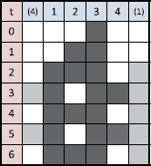

  

  State changes by Wolfram’s Rule 110 in Torus world

Due to these approximations, the number of possible state transitions can be made smaller in the case of elementary CAs like Fig. 3. Our learning framework can handle both limited frames and torus worlds by considering adequate state transitions representation as input. For example, to represent a torus world of size 4, a configuration is represented by a vector with 6 elements (0,1,2,3,4,5): 1,2,3,4 respectively represent their values in the corresponding cells, and 0,5 respectively represent the values of cells 4 and 1 (colored gray when the value is 1). This last information can be represented in a background theory as the two rules with the time argument:

$$\begin{array}{@{}l} c(0, t) \leftarrow c(4, t), \\ c(5, t) \leftarrow c(1, t), \end{array} $$

where c(x) represents a cell x and c(x,t) is its state at time step t. Unfortunately, these two rules do not have corresponding rules without the time argument, since the head literals refer the time step t instead of t+1. Hence, simple removal of the time argument from the both sides changes the dynamic meaning of the NLP in application of the T _P operator that infers about the next time step. Then, without the time argument, we should copy the rules for c(4) to those for c(0), and copy the rules for c(1) to those for c(5).

Now we use non-ground resolution and consider the following two biases (Sect. 5.3):

• Bias I: The body of each rule contains at most n neighbor literals.

• Bias II: The rules are universal for every time step and for any position. This means that the same states of the neighbor cells always implies the same state in the center cell at the next time step.

Combining these two biases, we can adapt LF1T to learn dynamics of CAs. Using Bias I, the rule construction process only considers n literals (here n=3) in the neighbors of the cell in the body of a rule. With Bias I, ground resolution is not sufficient to compare non-ground rules with ground rules, for that we need non-ground resolution. We apply anti-instantiation (AI) for getting universal rules with Bias II, whenever a newly added rule $R_{A}^{I}$ is not subsumed by any rule in the current program. We can guarantee the soundness of this generalization under Bias II. However, without Bias I, we cannot determine the body literals for construction of each universal rule, so that we must examine the effects from non-neighbor cells too.

Using Bias I only, LF1T in a limited frame of width 4 learns the following rules for Wolfram’s Rule 110:

$$ \begin{aligned}[c] &c(2) \leftarrow \neg c(2) \land c(3), \\ &c(3) \leftarrow \neg c(2) \land c(3), \\ &c(3) \leftarrow c(3) \land \neg c(4), \\ &c(x) \leftarrow \neg c(x-1) \land c(x+1), \\ &c(x) \leftarrow c(x-1) \land c(x) \land \neg c(x+1). \end{aligned} $$

(8)

Instead, when we use a torus world of length 4 for Wolfram’s Rule 110 in LF1T with Bias I only, Table 5 shows the learning process⁷ and the following NLP is obtained:

$$ \begin{aligned}[c] &c(3) \leftarrow c(3), \\ &c(3) \leftarrow c(4), \\ &c(x) \leftarrow \neg c(x) \land c(x+1), \\ &c(x) \leftarrow \neg c(x-1) \land c(x+1), \\ &c(x) \leftarrow c(x-1) \land c(x) \land \neg c(x+1). \end{aligned} $$

(9)

Both programs (8) and (9) are quite different from the original rules in Table 4. On the other hand, if we use Biases I and II in either a limited frame of width 4 or a torus world of length 4, we get the following NLP (the process is in Table 5), which are equivalent to the original transition rule in Table 4:

$$ \begin{aligned}[c] &c(x) \leftarrow c(x) \land \neg c(x+1), \\ &c(x) \leftarrow \neg c(x-1) \land c(x), \\ &c(x) \leftarrow \neg c(x-1) \land c(x+1), \\ &c(x) \leftarrow \neg c(x) \land c(x+1). \end{aligned} $$

(10)

In learning an NLP for Rule 110 with Biases I and II, we get interesting generalizations. The NLP obtained from the trace of Rule 110 with LF1T becomes more compact in 4 rules, whereas the original transition rule representing the dynamics of this CA in Table 4 consists of 5 rules. However, there still exists a redundancy here; we can omit either the second or the third rule from (10). As discussed in Sect. 6.1, LF1T does not currently provide a method to remove irredundant rules from the learned rules.

Table 5 LF1T algorithm with Bias I on Rule 110 in Torus world

Table 6 LF1T algorithm with Biases I and II on Rule 110 in Torus world

7 Related work

7.1 Learning from interpretations

As stated in Sect. 1, learning from interpretations (LFI) (De Raedt 1997) has been an ILP framework to produce a program from its interpretations. LFI considers examples simply as single interpretations that are supposed to be models of an output program, hence is different from LFIT, which takes pairs of interpretations as its input. We actually see that LFI is a special case of LFIT. That is, LFI can be constructed from LFIT as follows. Since $I\in 2^{\mathcal{B}}$ is a model of P iff T _P (I)⊆I, we can classify each example $(I,J)\in 2^{\mathcal{B}}\times 2^{\mathcal{B}}$ for LFIT into a positive example for LFI if J⊆I or a negative example for LFI otherwise. Note that information of J is only used to check if I is a model or not in this conversion.

Then, there is still a difference between the above LFI and the conventional LFI by De Raedt (1997). The setting for De Raedt’s LFI learns a clausal theory, i.e., a set of clauses, instead of an NLP that is a set of rules of the form (1). A clause is simply a disjunction of literals, while a positive literal and a negative literal in the body are clearly distinguished in a rule of an NLP. Other than this syntactical difference, the algorithm of conventional LFI can be used to construct a clausal theory from our input.

More generally, learning Boolean functions in the field of computational learning theory (Kearns and Vazirani 1994) is different from LFIT, since LFIT learns dynamics of systems as a set of Boolean functions appearing in Boolean networks, while the conventional learning setting is not involved in dynamics and often learns single Boolean functions. Similar to LFI, computational learning theories usually do not learn dynamics of systems in general.

7.2 Learning action theories

Learning action theories (Moyle 2003; Otero 2005; Inoue et al. 2005; Tran and Baral 2009; Corapi et al. 2011; Rodrigues et al. 2012) can be considered to share the common goals with LFIT on learning dynamics. Moyle (2003) uses an ILP technique to learn a causal theory based on event calculus (Kowalski and Sergot 1986), given examples of input-output relations. Otero (2005) uses logic programs based on situation calculus (McCarthy and Hayes 1969), and considers causal theories represented in logic programs. Inoue et al. (2005) induce causal theories represented in an action language given an incomplete action description and observations. Tran and Baral (2009) define an action language which formalizes causal, trigger and inhibition rules to model signaling networks, and learn an action description in this language, given a candidate set of possible abducible rules. Active learning of action models is proposed by Rodrigues et al. (2012) in a STRIPS-like language. Probabilistic logic programs to maximize the probabilities of observations are learned by Corapi et al. (2011) by employing parameter estimation to find the probabilities associated with each atom and rule.

Works on learning action theories suppose applications to robotics and bioinformatics. In many action theories, one action is assumed to be performed at a time, so its learning task becomes sequential for each example sequence. In LFIT, on the other hand, every rule is fired as long as its body is satisfied and update is synchronously performed at every ground atom. Moreover, the goal of learning action theories is not exactly the same as that of LFIT. In particular, LFIT can learn dynamics of systems with positive and negative feedbacks, which has not been considered much in the literature.

Džeroski et al. (2001)’s relational reinforcement learning (RRL) is a learning technique that combines reinforcement learning with ILP. As in (non-relational) reinforcement learning, RRL can take into account feedbacks from the learning process as rewards: Each time an observation is received, an action is chosen so that the state is changed with the reward associated. The goal of RRL is then to find a suitable sequence of transitions that maximize rewards. The merit to use ILP in RRL is to have a more expressive representation in states, actions and Q-functions. As the motivation of RRL is different from that of LFIT, our goal is not to find an optimal strategy for state transition but to learn the system’s dynamics itself. As for the treatment of positive and negative feedbacks, LFIT learns how such feedbacks can be represented by logic programs.

7.3 Learning nonmonotonic programs

Learning NLPs has been considered in ILP, e.g., (Sakama 2001), but most approaches do not take the LFI setting. The LFI setting in learning NLPs is seen in Sakama (2005). Our learning framework is different from these previous works (Sakama 2001, 2005). From the application point of view, NLPs are often used in planning and robotics domain, and hence the difference between previous work on learning action theories and LFIT is inherited to the comparison between previous setting of learning NLPs and LFIT. From the semantical viewpoint, there is an additional important difference: Previous work on learning NLPs is usually based on the stable model semantics (Gelfond and Lifschitz 1988), but LFIT learns NLPs under the supported model (or supported set) semantics (Inoue and Sakama 2012). Here we discuss practical differences between these two semantics.

The merit of the stable model semantics is that we can use state-of-the-art answer set solvers for computation of stable models. In Sakama and Inoue (2013), transition rules of CAs are represented in first-order NLPs, which consist of rules of the form (3) with the time argument. In this case, each NLP with the time argument becomes acyclic so the supported models and stable models coincide, and thus we can use answer set solvers for simulation of a CA. However, each answer set becomes infinite unless a time bound is set. On the other hand, the merit of the supported model semantics is that we can omit the time argument from a program and make it simpler. As discussed in Sect. 3, Boolean networks can be represented in propositional NLPs (Inoue 2011), but still we can simulate state transition by watching the orbits of the T _P operator. More importantly, attractors can be directly obtained with the supported model or the supported set semantics. This is not possible using the stable models of NLPs (without the time argument), since they ignore all positive feedback loops in the dynamics (Inoue 2011). The supported models of an NLP can also be obtained as the models of Clark’s completion of the program using modern SAT solvers. If we use answer set solvers for an NLP with the time argument, we can simulate the dynamics of the corresponding Boolean networks, but need to analyze each answer set to know when the same state is encountered twice by tracing the orbit from time to time.

7.4 Learning Boolean networks and cellular automata

Learning the dynamics of Boolean networks has been considered in Bioinformatics. Liang et al. (1998) proposed the REVEAL algorithm, which uses mutual information in information theory as a measure of interrelationships. In REVEAL, the maximum number of arguments of each Boolean function is assumed to deal with exponential growth of computational time. Akutsu et al. (2003) analyze the problem of identifying a genetic network from the data obtained by multiple gene disruptions and overexpressions with respect to the number of experiments. They show algorithms for identifying the underlying genetic network by such experiments, but their network model is a static Boolean network model in which expression levels of genes are statically determined, and is hence different from the standard Boolean network in which expression levels of genes change synchronously. Pal et al. (2005) constructs Boolean networks from a partial description of state transitions. This method is considered as a method to complete missing transitions in the state transition table. However, Boolean functions are not constructed for each node in Pal et al. (2005). Compared with these studies, our learning method is a complete algorithm to learn a set of logical state transition rules for a Boolean network. As in Pal et al. (2005), we can also deal with partial transitions (Sect. 5.4), but will not identify or enumerate all possible complete transitions. Akutsu et al. (2009) guess unknown Boolean functions of a Boolean network whose network topology is known. This corresponds to learning Boolean networks with the bias of neighbor nodes (Sect. 5.3). In Akutsu et al. (2009), only acyclic networks are considered, and the main focus is a computational analysis of such problems. Notably, all these previous works do not use ILP techniques.

In ILP, Srinivasan and Bain (2012) present a framework to learn Petri nets from state transitions. Petri nets can handle quantities of entities but their update schemes are different from those of Boolean networks. In Srinivasan and Bain (2012), a hierarchical Petri net can be obtained by iterative applications of their algorithm, but it is not possible to obtain networks with positive and negative feedback cycles. In fact, cyclic dependencies have been generally hard to be learned in ILP methods. Tamaddoni-Nezhad et al. (2006) combine abduction and induction to learn rules of concentration changes of a metabolite caused by changes in other metabolites in a metabolic pathway. This method gives an empirical way to learn some causal effects, but its application domain does not deal with dynamical effects of feedbacks, and a learned program does not describe complete transitions of the dynamical system. Inoue et al. (2013) complete causal networks by meta-level abduction. A biological network can be constructed with this method for an incomplete structure, but the abductive method does not consider dynamical behavior of the network and cannot deal with negative feedbacks.

In cellular automata (CAs), constructing transition rules from given configurations is known as the identification problem. Adamatzky (1994) provides algorithms for identifying different classes of CAs, and analyzes computational complexities of those algorithms. Several algorithms are also proposed in Adamatzky (2007). To the best of our knowledge, however, there is no algorithm which uses ILP techniques for identifying CA rules.

8 Conclusion and future work

Learning complex networks becomes more and more important, but it is hard to infer rules of systems dynamics due to presence of positive and negative feedbacks. We here firstly tackled the induction problem of such dynamical systems in terms of NLP learning from synchronous state transitions. The proposed algorithm LF1T has the following properties:

• Given any state transition diagram, which is either complete or partial, we can learn an NLP that exactly captures the system dynamics.

• Learning is performed only from positive examples, and produces NLPs that consist only of rules to make literals true.

• Generalization on state transition rules is done by resolution, in which each rule can only be replaced by a general rule. As a result, an output NLP is as minimal as possible with respect to the size of each rule, but may contain redundant rules.

We have also shown how to incorporate background knowledge and inductive biases, and have applied the framework to learning transition rules of Boolean networks and cellular automata. The results are promising, and implemented programs can be useful for designing the state transition rules of dynamical systems from a specification of desired or non-desired state transition diagrams. For instance, a system can be considered to be robust if it is tolerant to a perturbation (or an exogenous event, see Sect. 5.2) which interferes normal state transition. Such a transition diagram could be designed as a tree shape, in which its root node corresponds to an attractor, so that any forced state change is eventually recovered to reach to the attractor (Li et al. 2004). Then we can do reverse engineering to get the corresponding state transition rules for the Boolean network.

A promising optimization of the implementation will be to use binary decision diagrams (BDDs) (Bryant 1986) to represent the rules of an NLP P in a compressed way. This data structure will be more efficient with regard to memory and search spaces. With such representation, we can divide the complexity of learning step transitions by n: For one transition the algorithm learn n rules with the same body, if we use heads as leaves of the BDD, bodies of these rules will be learned and represented in only one multi-terminal BDD.

More complex schemes such as asynchronous and probabilistic updates (Shmulevich et al. 2002; Garg et al. 2008) do not obey transition by the T _P operator. Not only Boolean but multiple-state dynamical systems have been considered in the literature, so learning such systems is a future work. Cellular automata with asynchronous or probabilistic updates and their identification methods have also been proposed (Adamatzky 1994). Those nondeterministic transition systems are more tolerant to noise, so can be expected to be applied to real-world dynamical systems, but have not yet been sufficiently connected to existing work on symbolic inference systems. Learning such dynamical networks by extending the algorithms in this paper is thus an important future work. Probabilistic logic learning would be useful for such learning tasks.

References

Adamatzky, A. (1994). Identification of cellular automata. Boca Raton: CRC Press.
Adamatzky, A. (Ed.) (2007). Identification of cellular automata. Special issue of Journal of Cellular Automata, 2(1).
Akutsu, T., Kuhara, S., Maruyama, O., & Miyano, S. (2003). Identification of genetic networks by strategic gene disruptions and gene overexpressions under a Boolean model. Theoretical Computer Science, 298, 235–251.
Akutsu, T., Tamura, T., & Horimoto, K. (2009). Completing networks using observed data. In LNAI: Vol. 5809. Proceedings of ALT ’09 (pp. 126–140). Berlin: Springer.
Apt, K. R., & Bezem, M. (1991). Acyclic programs. New Generation Computing, 9, 335–363.
Apt, K. R., Blair, H. A., & Walker, A. (1988). Towards a theory of declarative knowledge. In J. Minker (Ed.), Foundations of deductive databases and logic programming (pp. 89–148). San Mateo: Morgan Kaufmann.
Baral, C., Eiter, T., Bjäreland, M., & Nakamura, M. (2008). Maintenance goals of agents in a dynamic environment: formulation and policy construction. Artificial Intelligence, 172(12/13), 1429–1469.
Blair, H. A., Chidella, J., Dushin, F., Ferry, A., & Humenn, P. (1997). A continuum of discrete systems. Annals of Mathematics and Artificial Intelligence, 21, 153–186.
Bryant, R. (1986). Graph-based algorithms for Boolean function manipulation. IEEE Transactions on Computers, 35(8), 677–691.
Chaos, A., Aldana, M., Espinosa-Soto, C., Ponce de Léon, B., Arroyo, A. G., & Alvarez-Buylla, E. R. (2006). From genes to flower patterns and evolution: dynamic models of gene regulatory networks. Journal of Plant Growth Regulation, 25(4), 278–289.
Clark, K. L. (1978). Negation as failure. In H. Gallaire & J. Minker (Eds.), Logic and data bases (pp. 119–140). New York: Plenum.
Corapi, D., Sykes, D., Inoue, K., & Russo, A. (2011). Probabilistic rule learning in nonmonotonic domains. In LNAI: Vol. 6814. Computational logic in multi-agent systems: proceedings of the 12th international workshop (CLIMA-XII) (pp. 243–258). Berlin: Springer.
Davidich, M. I., & Bornholdt, S. (2008). Boolean network model predicts cell cycle sequence of fission yeast. PLoS ONE, 3(2), e1672.
De Raedt, L. (1997). Logical settings for concept-learning. Artificial Intelligence, 95, 187–201.
Dubrova, E., & Teslenko, M. (2011). A SAT-based algorithm for finding attractors in synchronous Boolean networks. IEEE/ACM Transactions on Computational Biology and Bioinformatics, 8(5), 1393–1399.
Džeroski, S., De Raedt, L., & Driessens, K. (2001). Relational reinforcement learning. Machine Learning, 43, 7–52.
Fauré, A., Naldi, A., Chaouiya, C., & Thieffry, D. (2006). Dynamical analysis of a generic Boolean model for the control of the mammalian cell cycle. Bioinformatics, 22(14), e124–e131.
Garg, A., Di Cara, A., Xenarios, I., Mendoza, L., & De Micheli, G. (2008). Synchronous versus asynchronous modeling of gene regulatory networks. Bioinformatics, 24(17), 1917–1925.
Gelfond, M., & Lifschitz, V. (1988). The stable model semantics for logic programming. In Proceedings of ICLP ’88 (pp. 1070–1080). Cambridge: MIT Press.
Inoue, K. (2011). Logic programming for Boolean networks. In Proceedings of IJCAI-11 (pp. 924–930). Menlo Park: AAAI Press.
Inoue, K., & Sakama, C. (2012). Oscillating behavior of logic programs. In E. Erdem, J. Lee, Y. Lierler, & D. Pearce (Eds.), LNAI: Vol. 7265. Correct reasoning—essays on logic-based AI in honour of Vladimir Lifschitz (pp. 345–362). Berlin: Springer.
Inoue, K., Bando, H., & Nabeshima, H. (2005). Inducing causal laws by regular inference. In LNAI: Vol. 3625. Proceedings of ILP ’05 (pp. 154–171). Berlin: Springer.
Inoue, K., Doncescu, A., & Nabeshima, H. (2013). Completing causal networks by meta-level abduction. Machine Learning, 91(2), 239–277.
Kauffman, S. A. (1993). The origins of order: self-organization and selection in evolution. Oxford: Oxford University Press.
Kearns, M. J., & Vazirani, U. V. (1994). An introduction to computational learning theory. Oxford: MIT Press.
Kowalski, R. A., & Sergot, M. J. (1986). A logic-based calculus of events. New Generation Computing, 4(1), 67–95.
Li, F., Long, T., Lu, Y., Ouyang, Q., & Tang, C. (2004). The yeast cell-cycle network is robustly designed. Proceedings of the National Academy of Sciences of the United States of America, 101(14), 4781–4786.
Liang, S., Fuhrman, S., & Somogyi, R. (1998). REVEAL, a general reverse engineering algorithm for inference of genetic network architectures. In Pacific symposium on biocomputing (Vol. 3, pp. 18–29).
Marek, W., & Subrahmanian, V. S. (1992). The relationship between stable, supported, default and autoepistemic semantics for general logic programs. Theoretical Computer Science, 103(2), 365–386.
McCarthy, J., & Hayes, P. J. (1969). Some philosophical problems from the standpoint of artificial intelligence. In B. Meltzer & D. Michie (Eds.), Machine intelligence (Vol. 4, pp. 463–502). Edinburgh: Edinburgh University Press.
Moyle, S. (2003). Using theory completion to learn a robot navigation control programs. In LNAI: Vol. 2583. Proceedings of ILP ’02 (pp. 182–197). Berlin: Springer.
Muggleton, S. H., De Raedt, L., Poole, D., Bratko, I., Flach, P., Inoue, K., & Srinivasan, A. (2012). ILP turns 20—biography and future challenges. Machine Learning, 86(1), 3–23.
Otero, R. P. (2005). Induction of the indirect effects of actions by monotonic methods. In LNAI: Vol. 3625. Proceedings of ILP ’05 (pp. 279–294). Berlin: Springer.
Pal, R., Ivanov, I., Datta, A., Bittner, M. L., & Dougherty, E. R. (2005). Generating Boolean networks with a prescribed attractor structure. Bioinformatics, 21(21), 4021–4025.
Plotkin, G. D. (1970). A note on inductive generalization. In B. Meltzer & D. Michie (Eds.), Machine intelligence (Vol. 5, pp. 153–163). Edinburgh: Edinburgh University Press.
Remy, E., & Ruet, P. (2008). From elementary signed circuits to the dynamics of Boolean regulatory networks. Bioinformatics, 24, 220–226.
Robinson, R. A. (1965). A machine-oriented logic based on the resolution principle. Journal of the ACM, 12, 23–41.
Rodrigues, C., Gérard, P., Rouveirol, C., & Soldano, H. (2012). Active learning of relational action models. In LNAI: Vol. 7207. Proceedings of ILP ’11 (pp. 302–316). Berlin: Springer.
Sakama, C. (2001). Nonmonotonic inductive logic programming. In LNAI: Vol. 2173. Proceedings of LPNMR ’01 (pp. 62–80). Berlin: Springer.
Sakama, C. (2005). Induction from answer sets in nonmonotonic logic programs. ACM Transactions on Computational Logic, 6(2), 203–231.
Sakama, C., & Inoue, K. (2013). Abduction, unpredictability and Garden of Eden. Logic Journal of the IGPL. doi:10.1093/jigpal/jzt015.
Shmulevich, I., Dougherty, E. R., Kim, S., & Zhang, W. (2002). Probabilistic Boolean networks: a rule-based uncertainty model for gene regulatory networks. Bioinformatics, 18(2), 261–274.
Srinivasan, A., & Bain, M. (2012). Knowledge-guided identification of Petri net models of large biological systems. In LNAI: Vol. 7207. Proceedings of ILP ’11 (pp. 317–331). Berlin: Springer.
Tamaddoni-Nezhad, A., Chaleil, R., Kakas, A., & Muggleton, S. (2006). Application of abductive ILP to learning metabolic network inhibition from temporal data. Machine Learning, 65, 209–230.
Tran, N., & Baral, C. (2009). Hypothesizing about signaling networks. Journal of Applied Logic, 7(3), 253–274.
van Emden, M. H., & Kowalski, R. A. (1976). The semantics of predicate logic as a programming language. Journal of the ACM, 23(4), 733–742.
Wolfram, S. (1994). Cellular automata and complexity: collected papers. Boulder: Westview.
Author information
Authors and Affiliations
Corresponding author
Additional information
Editors: Fabrizio Riguzzi and Filip Zelezny.
This research was supported in part by the NII research project on “Dynamic Constraint Networks” and by the “Systems Resilience” project at Research Organization of Information and Systems, Japan.
Rights and permissions
About this article
Cite this article
Inoue, K., Ribeiro, T. & Sakama, C. Learning from interpretation transition. Mach Learn 94, 51–79 (2014). https://doi.org/10.1007/s10994-013-5353-8
Received:
Accepted:
Published:
Issue Date:
DOI: https://doi.org/10.1007/s10994-013-5353-8