Polynomial-time inverse computation for accumulative functions with multiple data traversals

Abstract

The problem of inverse computation has many potential applications such as serialization/deserialization, providing support for undo, and test-case generation for software testing. In this paper, we propose an inverse computation method that always terminates for a class of functions known as parameter-linear macro tree transducers, which involve multiple data traversals and the use of accumulations. The key to our method is the observation that a function in the class can be regarded as a non-accumulative context-generating transformation without multiple data traversals. Accordingly, we demonstrate that it is easy to achieve terminating inverse computation for the class by context-wise memoization of the inverse computation results. We also show that when we use a tree automaton to express the inverse computation results, the inverse computation runs in time polynomial to the size of the original output and the textual program size.

1 Introduction

The problem of inverse computation [1, 2, 20, 21, 23, 30, 37, 40, 49]—finding an input s for a program f and a given output t such that f(s)=t—has many potential applications, including test-case generation in software testing, supporting undo/redo, and obtaining a deserialization from a serialization program.

Let us illustrate the problem with an example. Suppose that we want to write an evaluator for a simple arithmetic expression language defined by the following datatype. (We basically follow the Haskell syntax [6] even though we target an untyped first-order functional language with call-by-value semantics.)

Informally, Z and Zero represent 0, One represents 1, S(n) means n+1 (the successor of n), Add(n ₁,n ₂) adds the numbers n ₁ and n ₂, and Dbl(n) doubles the number n.

An evaluator eval::Exp→Val of the expressions can be implemented as follows.

Here, eval uses evalAcc that uses accumulations. The function evalAcc satisfies the invariant that evalAcc(e,m)=eval(e)+m, where “+” is the addition operator for values. This invariant enables us to read the definition intuitively; e.g., the case of Dbl can be read as eval(Dbl(x))+y=eval(x)+eval(x)+y.

The inverse computation of eval, which enumerates the inputs for a given t, is sometimes useful for testing computations on E. For example, suppose that we write an optimizer f that converts all the expressions e satisfying $\mathit {eval} (e) = \mathsf {S} ^{2^{n}}( \mathsf {Z} )$ into Dbl ⁿ(One), and we want to test if the optimizer works correctly or not, i.e., whether $\mathit {eval} (e) = \mathsf {S} ^{2^{n}}( \mathsf {Z} )$ implies f(e)=Dbl ⁿ(One) or not.¹ A solution would involve randomly generating or enumerating expressions e, filtering out the es that do not satisfy $\mathit {eval} (e) = \mathsf {S} ^{2^{n}}( \mathsf {Z} )$, and checking f(e)=Dbl ⁿ(One). However, it is unsatisfactory because it is inefficient; the majority of the expressions do not evaluate to $\mathsf {S} ^{2^{n}}( \mathsf {Z} )$. Inverse computation enables us to generate only the test-cases that are relevant to the test. A test with inverse computation can be efficiently performed by (1) picking up a number m of the form $\mathsf {S} ^{2^{n}}( \mathsf {Z} )$, (2) picking up an expression e from the set obtained from the inverse computation for m, and (3) checking if the optimizer f converts e into Dbl ⁿ(One). Here, all the picked up (randomly generated or enumerated) data are relevant to the final check in the Step (3). Lazy SmallCheck [43] and EasyCheck [9] use inverse computation for efficient test-case generation, which of course has to be supported by efficient inverse computation.

However, there are as yet no systematic efficient inverse computation methods that can handle eval. One reason is that evalAcc contains accumulations and multiple data traversals. It is so far unclear how to perform tractable terminating inverse computation for functions with accumulations and multiple data traversals (Sect. 2). Some of the existing methods [1, 2, 21, 37] do not terminate for functions with  accumulations.  Some  approaches [20, 39, 40] can handle certain accumulative computations efficiently, but they do not work for non-injective functions such as eval. Although some inverse computation methods terminate for accumulative functions [17, 32], the complexity upper bound is unclear when there are also multiple data traversals.

In this paper, we propose an inverse computation method that can handle a class of accumulative functions like eval that have multiple data traversals, namely deterministic macro tree transducers [15] with the restriction of parameter-linearity (Sect. 3). In this class of functions, variables for accumulation (such as y in evalAcc) cannot be copied but inputs (such as x, x ₁ and x ₂ in evalAcc) can be traversed in many times (as x). Our method computes the set as a tree automaton [10] for a given function f and an output y in time polynomial to the size of y (Sect. 4). The key to our inverse computation is the observation that a program in the parameter-linear macro tree transducers is indeed a non-accumulative transformation that generates contexts (i.e., trees with holes) without multiple data traversals. From this viewpoint, we can do the inverse computation through a variant of the existing inverse computation methods [1, 2, 4]. Note that viewing a program as a context-generating transformation is not new. What is new in our paper is to use this view to achieve polynomial-time inverse computation for the class of accumulative functions with multiple data traversals.

Our main contributions are summarized as follows.

• We demonstrate that simply viewing a function as a context-generating transformation helps us to achieve a systematic inverse computation method for accumulative functions. After converting a program into a context-generating one, it is easy to perform inverse computation for the program.

• We show that, for parameter-linear macro tree transducers, our inverse computation method runs in time polynomial to the size of the output and the textual program size, and in time exponential to the number of the functions in the program.

The rest of the paper is organized as follows. Section 2 shows an overview of our proposal. Section 3 defines the target language, parameter-linear macro tree transducers. Section 4 formally presents our inverse computation method. Section 5 reports and discusses the experimental results with our prototype implementation. Section 6 shows four extensions of our proposal, and Sect. 7 shows the relationship between ours and the other research. Section 8 concludes the paper and outlines future work.

The preliminary version of this article has appeared in [36]. The main difference from the version is that we have implemented the proposed algorithm and performed some experiments (Sect. 5). We also have added discussions on the two further extensions of our proposed method (Sects. 6.3 and 6.4) and some explanations in several places.

2 Overview

In this section, we give a brief overview of our proposal.

2.1 Review: when inverse computation terminates

Let us begin with an illustrative example showing when a simple inverse computation [1, 4] terminates. The following function parity takes a natural number n and returns nmod2.

What should we do for inverse computation of parity given an original output t? Abramov and Glück [1, 2] used a symbolic computation method called (needed) narrowing² [4] as a simple way to find a substitution θ such that $\mathit {parity} (x)\theta \stackrel {?}{=}t$, where $\stackrel {?}{=}$ represents an equivalence check of (first-order) values defined in a standard way (e.g., $\mathsf {Z} \stackrel {?}{=} \mathsf {Z} \equiv \top$). The same idea is also shared among logic programming languages such as Curry and Prolog.³ Roughly speaking, a narrowing is a substitution followed by a reduction, and it can reduce an expression with free variables. For example, parity(x) is not reducible, but, if we substitute Z to x, we can reduce the expression to Z. Such a reduction after a substitution is a narrowing that can be written as parity(x)⇝ _x↦Z Z. The notion can naturally be extended to equivalence checks, such as $( \mathit {parity} (x) \stackrel {?}{=} \mathsf {Z} ) \leadsto_{x \mapsto \mathsf {Z} } ( \mathsf {Z} \stackrel {?}{=} \mathsf {Z} ) \equiv \top$. By using narrowing, we can obtain the corresponding input by collecting the substitutions used in the narrowing. For example, consider the inverse computation of parity for an output Z. Since we have⁴

we know that parity(Z)=Z, and since we have

we know that parity(S(S(Z)))=Z.

Sometimes, the simple inverse computation does not terminate; this happens especially when we give it an output that has no corresponding inputs. For example, the simple inverse computation of parity for an output S(S(Z)) runs infinitely:

$$\begin{aligned} ( \mathit {parity} (x) \stackrel {?}{=} \mathsf {S} ^2( \mathsf {Z} )) \leadsto_{x \mapsto \mathsf {S} (x)}& ( \mathit {aux} (x) \stackrel {?}{=} \mathsf {S} ^2( \mathsf {Z} )) \\ \leadsto_{x \mapsto \mathsf {S} (x)}& ( \mathit {parity} (x) \stackrel {?}{=} \mathsf {S} ^2( \mathsf {Z} )) \leadsto_{x \mapsto \mathsf {S} (x)} \dots \end{aligned}$$

One might notice that the check $( \mathit {parity} (x) \stackrel {?}{=} \mathsf {S} ^{2}( \mathsf {Z} ))$ occurs twice in the sequence.

Actually, with memoization, the simple inverse computation for parity always terminates. For the above narrowing sequence, by memoizing all the checks in the sequence, we can tell that the same check $( \mathit {parity} (x) \stackrel {?}{=} \mathsf {S} ^{2}( \mathsf {Z} ))$ occurs twice, and hence the narrowing sequence cannot produce any result. In general, the number of equality checks occurring in the inverse computation is finite because it always has the form $f(x) \stackrel {?}{=}t$ (up to α-renaming), where t is a subterm of the original output given to the inverse computation. Thus, the simple inverse computation always terminates with memoization for parity.

This observation also gives an upper bound of the worst-case complexity of inverse computation of parity; it runs in constant time regardless the size of the original output because the checks in the narrowing have the form of either $\mathit {parity} (x) \stackrel {?}{=}t$ or $\mathit {aux} (x) \stackrel {?}{=}t$, only where t is the original output.

2.2 Problem: non-termination due to accumulations and multiple data traversals

Consider a simplified version of eval:

Though simplified, this function still contains the challenging issues: accumulations and multiple data traversals. Since we have for example, the inverse computation of ev for S ²(Z) should result in the set above.

Unlike parity, the simple inverse computation method does not always terminate. For example, the simple inverse computation of ev for Z does not terminate.

$$\begin{aligned} ( \mathit {ev} (x) \stackrel {?}{=} \mathsf {Z} ) &\leadsto ( \mathit {evA} (x, \mathsf {Z} ) \stackrel {?}{=} \mathsf {Z} ) \\ &\leadsto _{x \mapsto \mathsf {Dbl} (x)} ( \mathit {evA} (x, \mathit {evA} (x, \mathsf {Z} )) \stackrel {?}{=} \mathsf {Z} ) \leadsto _{x \mapsto \mathsf {Dbl} (x)} \dots \end{aligned}$$

Memoization is no longer useful for making the simple inverse computation terminate because there are no repeated checks in the infinite sequence.

The following issues make it difficult for the inverse computation to terminate and even harder to run it in polynomial time.

• Accumulations, a sort of call-time computation commonly used in tail recursion, increase the size of the terms in the narrowing process. For example, evA contains the accumulations

  $$\mathit {evA} ( \mathsf {Dbl} (x),y) = \mathit {evA} (x,\underline{ \mathit {evA} (x,y)}) $$

  which increase the term-size in the following narrowing steps.

  $$( \mathit {evA} (x,\underline{ \mathsf {Z} }) \stackrel {?}{=} \mathsf {Z} ) \leadsto _{x \mapsto \mathsf {Dbl} (x)} ( \mathit {evA} (x,\underline{ \mathit {evA} (x, \mathsf {Z} )}) \stackrel {?}{=} \mathsf {Z} ) $$

  We can see that the second argument of evA (underlined above) gets bigger in narrowing.

• Multiple data traversals make things much worse. It prevents us from considering function calls separately. For example, we have to track the two calls $\underline{ \mathit {evA} (x,\underline{ \mathit {evA} (x,y)}})$ simultaneously. We can see that the number of function calls we have to track simultaneously increases in narrowing. To clarify the problem caused by multiple data traversals, we will look at the issue of accumulations in the absence of multiple data traversals. Suppose that ev does not have the case for Dbl and thus does not contain multiple data traversals. Although there are still an infinite narrowing sequence

  $$\begin{aligned} ( \mathit {ev} (x) \stackrel {?}{=} \mathsf {Z} )& \leadsto ( \mathit {evA} (x, \mathsf {Z} ) \stackrel {?}{=} \mathsf {Z} ) \\ &\leadsto _{x \mapsto \mathsf {Add} (x_1,x_2)} ( \mathit {evA} (x_1, \mathit {evA} (x_2, \mathsf {Z} )) \stackrel {?}{=} \mathsf {Z} ) \leadsto \dots\mbox{,} \end{aligned}$$

  one can make the simple inverse computation terminate by decomposing the check $( \mathit {evA} (x_{1}, \mathit {evA} (x_{2}, \mathsf {Z} )) \stackrel {?}{=} \mathsf {Z} )$ into $\mathit {evA} (x_{1},z) \stackrel {?}{=} \mathsf {Z} \wedge \mathit {evA} (x_{2}, \mathsf {Z} ) \stackrel {?}{=}z$ and by observing that, for $\mathit {evA} (x_{1},z) \stackrel {?}{=}z'$, we only need to consider the substitutions that map z and z′ to subterms of the output fed to the inverse computation, i.e., Z. Thus, we can substitute a concrete subterm to z and check $\mathit {evA} (x_{1}, \mathsf {Z} ) \stackrel {?}{=}t$ and $\mathit {evA} (x_{2},t) \stackrel {?}{=} \mathsf {Z}$ separately for a concrete t (a more refined idea can be found in [17, 32]), and we can bound the complexity of inverse computation in a similar way as we did for parity. However, this idea does not scale for functions with multiple data traversals, in which many function calls are tracked simultaneously in narrowing. Although the existing approaches [17, 32] achieve terminating inverse computation of certain accumulative functions with multiple data traversals, it is unclear whether there are polynomial-time inverse computations for functions with multiple data traversals.

2.3 Our idea

One might have noticed that the result of evA(s,t) can be written as K _s [t] whatever t is, where K _s is a context (i.e., a tree with holes like S(•)) determined by s and K _s [t] is the tree obtained from K _s by replacing • with t. For example, we have $\mathit {evA} ( \mathsf {One} ,\underline{ \mathsf {Z} }) = \mathsf {S} (\underline{ \mathsf {Z} })$, $\mathit {evA} ( \mathsf {One} ,\underline{ \mathsf {S} ( \mathsf {Z} )}) = \mathsf {S} (\underline{ \mathsf {S} ( \mathsf {Z} )})$, where we have underlined the hole position of the context. More generally, for a context K _One =S(•), we have evA(One,t)=K _One [t] for any t. Thus, we can define a context-generating version evA _c of evA that satisfies evA _c(One)=S(•), for example. The functions ev _c and evA _c can be defined as follows.

There are no accumulations or multiple data traversals. That is, evA _c is indeed a non-accumulative and input-linear context-generating transformation. Note that ev _c(x)=ev(x) holds for any x.

Now the simple inverse computation terminates again. For example, the inverse computation of ev _c for S ²(Z) is as follows.

The only difference is that now $\stackrel {?}{=}$ takes care of the contexts. Notice that the checks occurring in the narrowing have the form $f_{\mathrm {c}}(x) \stackrel {?}{=}K$, where K is a subcontext of the original output. Since this generally holds for ev _c, the termination property of the simple inverse computation is now recovered.

Besides the new point of view, our approach also involves a new way to express the memoized narrowing computation. Instead of using (a variant of) the existing method directly, we use a tree automaton [10]; it is more suitable for a theoretical treatment than side-effectful memoized narrowing, and can express an infinite set of inputs (note that in general the number of corresponding inputs is infinite as in the case of parity). For example, the inverse computation of ev _c for S ²(Z) can be expressed by the following automaton where each state is of the form $q_{f^{-1}(K)}$.

Note that $f(x) \stackrel {?}{=}K$ can be regarded as $x \stackrel {?}{=}f^{-1}(K)$. We write $q_{f^{-1}(K)}$ for a state instead of $q_{f(x) \stackrel {?}{=}K}$ because an automaton constructed in this way can be regarded as all the possible reductions starting with f ⁻¹(K). This automaton contains the state $q_{ \mathit {evA} _{\mathrm {c}}^{-1}({\bullet })}$ that accepts no trees, which intuitively means that the evaluation of $\mathit {evA} _{\mathrm {c}}^{-1}({\bullet })$ fails; i.e., the narrowing from $\mathit {evA} _{\mathrm {c}}(x) \stackrel {?}{=}{\bullet }$ fails. The size of the resulting automaton is bounded linearly by the size of the original output of ev. It is also worth noting that we can extract a tree from an automaton in time linear to the size of the automaton [10].

All of the above results are obtained by just a simple observation: a program like ev is a non-accumulative context-generating transformation without multiple data traversals.

3 Target language

In this section, we formally describe the programs we target, which are written in an (untyped) first-order functional programming language with certain restrictions.

3.1 Values: trees

The values of the language are trees consisting of constructors (i.e., a ranked alphabet).

Definition 1

(Trees)

A set of trees $\mathcal {T}_{\varSigma }$ over constructors Σ is defined inductively as follows: for every σ∈Σ ⁽⁰⁾, $\sigma \in \mathcal {T}_{\varSigma }$, and for every σ∈Σ ⁽ⁿ⁾ and $t_{1}, \ldots, t_{n} \in \mathcal {T}_{\varSigma }$ (n>0), $\sigma(t_{1},\dots,t_{n}) \in \mathcal {T}_{\varSigma }$, where Σ ⁽ⁿ⁾ is the set of the constructors with arity n.

For constructors Z,Zero,One,Nil∈Σ ⁽⁰⁾, S∈Σ ⁽¹⁾ and Cons,Add∈Σ ⁽²⁾, examples of trees are S(Z), Cons(Z,Nil), and Add(Add(Zero,One),Zero). We shall fix the set Σ of the constructors throughout the paper for simplicity of presentation. The size of a tree t is the number of the constructor occurrences in t. For example, the size of S(Z) is 2.

In what follows, we shall use vector notation: $\overline {t}$ represents a sequence t ₁,…,t _n and $|\overline {t}|$ denotes its length n.

3.2 Programs: macro tree transducers

The syntax of the language is shown in Fig. 1. A program consists of a set of rules, and each rule has the form of either f(σ(x ₁,…,x _n ),y ₁,…,y _m )=e or f(x,y ₁,…,y _m )=e. There are two kinds of variable: input and output. Input variables, denoted by x in Fig. 1, can be decomposed by pattern-matching but cannot be used to compose a result. Output variables, denoted by y in Fig. 1, can be used to compose a result but cannot be decomposed. Output variables are sometimes called (accumulation) parameters. A program in the language is nothing but a (stay) macro tree transducer (MTT) [15]. Thus, a program written in the target language is called an MTT in this paper.

Fig. 1

Syntax of the target language: σ is an n-ary constructor, and f is an (m+1)-ary function

Example 1

(reverse)

A simple example of an accumulative function written in the target language is reverse. The following function reverse reverses a list of natural numbers expressed by S and Z.

The function nat just copies an input. This function is necessary because we prohibit using an input directly to produce a result in the language (see Fig. 1).

Example 2

(eval)

The eval program in Sect. 1 is an example of an MTT program. So is its simplified version ev.

Example 3

(mirror)

The following function mirror mirrors a list.

We omit the rules for rev and nat because they are the same as those in Example 1. Unlike ev and eval, mirror traverses an input twice with the different functions (app and rev). The function app is the so-called “append” function.

The size of a program is defined by the total number of function, constructor, and variable occurrences in the program. The intuition behind this definition is to approximate the size of program code in text. Note that the number of function or constructor occurrences is different from the number of functions or constructors. For example, the number of functions in reverse is 3, whereas the number of function occurrences is 9.

The language has a standard call-by-value semantics, as shown in Fig. 2. A judgment Γ;Δ⊢e↓t means that under an input-variable environment Γ and output-variable environment Δ, an expression e is evaluated to a value t. Programs are assumed to be deterministic; i.e., for each f, either f has at most one rule of the form f(x,y ₁,…,y _m )=e or has at most one rule of the form f(σ(x ₁,…,x _n ),y ₁,…,y _m )=e for each σ. The semantics of a function f is defined by

Note that we allow partial functions; e.g., we have [[nat]](Nil)=⊥. We shall sometimes abuse the notation and simply write f for [[f]]. The semantics is nothing but IO-production [15].

Fig. 2

Call-by-value semantics of the target language: here, we abuse the notation to write for where $n = |\overline {x}| = |\overline {s}|$

In addition, we also assume that programs are nondeleting, i.e., every input variable must occur in the corresponding right-hand-side expression. This restriction does not change the expressiveness; we can convert any program to one satisfying this restriction by introducing the function ignore satisfying [[ignore]](s,t)=t for any s and t and defined by ignore(σ(x ₁,…,x _n ),y)=ignore(x ₁,…ignore(x _n ,y)…) for every σ∈Σ. The restriction simplifies the discussions in Sects. 4.3, 6.1 and 6.2. All the previous examples are deterministic and nondeleting.

A program is called parameter-linear if every output variable y occurring on the left-hand side occurs exactly once on the corresponding right-hand side of each rule.⁵ All the previous examples are parameter-linear. Our polynomial time inverse computation depends on parameter-linearity.

4 Polynomial-time inverse computation

In this section, we formally describe our inverse computation. As briefly explained in Sect. 2, first, we convert an MTT program into a non-accumulative context-generating program (a program that generates contexts instead of trees) without multiple data traversals, such as ev _c in Sect. 2.3. Then, we perform inverse computation with memoization. More precisely, we construct a tree automaton [10] that represents the inverse computation result, whose run implicitly corresponds to (a context-aware version of) the existing inverse computation process with memoization [1, 4].

Our inverse computation consists of three steps:

• 1. We convert a parameter-linear MTT into a non-accumulative context-generating program.

• 2. We apply tupling [8, 25] to eliminate multiple data traversals.

• 3. We construct a tree automaton that represents the inverse computation result.

The first two steps are to obtain a non-accumulative context-generating program without multiple data traversals. The third step represents memoized inverse computation. The rest of this section explains each step in detail.

4.1 Conversion to context-generating program

The first and most important step is to convert an MTT program into a non-accumulative context-generating program. This transformation is also useful for removing certain multiple data traversals, as shown in the example of ev in Sect. 2. Moreover, this makes it easy to apply tupling [8, 25] to programs. Note that viewing MTT programs as non-accumulative context-generating transformations is not a new idea (see Sect. 3.1 of [12] for example). The semantics of the context-generating programs shown later is nothing but using Lemma 3.4 of [12] to evaluate MTT programs.

First, we will give a formal definition of contexts.

Definition 2

An (m-hole) context K is a tree in where •₁,…,• _m are nullary symbols such that ${\bullet }_{1},\ldots,{\bullet }_{m} \not\in \varSigma$.

An m-hole context K is linear if each • _i (1≤i≤m) occurs exactly once in K. We write K[t ₁,…,t _m ] for the tree obtained by replacing • _i with t _i for each 1≤i≤m. For example, K=Cons(•₁,•₂) is a 2-hole context and K[Z,Nil] is the tree Cons(Z,Nil). For 1-hole contexts, •₁ is sometimes written as •.

We showed that ev is indeed a non-accumulative context-generating transformation in Sect. 2. In general, any MTT program can be regarded as a non-accumulative context-generating transformation in the sense that, since output variables cannot be pattern-matched, the values bound to the output variables appear as-is in the computation result. Formally, we can state the following fact (Engelfriet and Vogler [15]; Lemma 3.19).

Fact 1

${\mathopen {[\![}f\mathclose {]\!]}}(s,\overline {t}) = t$ if and only if there is K such that ${\mathopen {[\![}f\mathclose {]\!]}}(s,\overline {{\bullet }}) = K$ and $t = K[\overline {t}]$.

Accordingly, we can convert an MTT program into a non-accumulative context-generating program, as shown below.

As a result of the above, in a converted program, the arguments of every function are variables, and the return value of a function cannot be traversed again. This rules out any accumulative computation.

The algorithm above is very similar to that used for deaccumulation [19, 31]. Unlike deaccumulation, we treat contexts as first-class objects, which enables us to adopt special treatment for contexts in our inverse computation method.

Example 4

(reverse)

The reverse program is converted into the following program.

The converted program has no accumulative computation.

Example 5

(eval)

The eval program in Sect. 1 is converted into the following program.

Note that the two occurrences of the function call evalAcc(x,…) on the right-hand side of the rule evalAcc(Dbl(x))=… are unified into the single call k=evalAcc _c(x). Recall that Algorithm 1 generates a new variable k _f,x for a pair of a function f and its input x, but not for its occurrence. Applying the same function to the same input results in the same context in a context-generating program, even though different accumulating arguments are passed in the original program. As a side effect, certain multiple data traversals, i.e., traversals of the same input by the same function, are eliminated through this conversion.

Example 6

(mirror)

The mirror program in Sect. 3 is converted into the following program.

We have omitted the definitions of rev _c and nat _c because they are the same as in Example 4. Some multiple data traversals still remain as k ₁=app _c(x),k ₂=rev _c(x). However, thanks to the conversion, this sort of multiple data traversal is easy to eliminate by tupling [8, 25] (see the next subsection).

For formal discussion, we define the syntax and the semantics of the non-accumulative context-generating programs in Fig. 3. Since contexts are bound to context variables k, the semantics uses second-order substitutions [12] that are mappings from variables to contexts. The application eΘ of a second-order substitution Θ to a term e is inductively defined by: σ(e ₁,…,e _n )Θ=σ(e ₁ Θ,…,e _n Θ) and k[e ₁,…,e _n ]Θ=K[e ₁ Θ,…,e _n Θ] where K=Θ(k). Similarly to MTT, we write [[f]] for the semantics of f.

Fig. 3

Syntax and semantics of the converted programs: here, we abuse the notation to write $\overline {k = g(z)}$ for sequence k ₁=g ₁(z ₁),…,k _l =g _l (z _l ) where l=|seqk=g(z)| and write as in Fig. 2

Now, we can show that the conversion is sound; it does not change the semantics of the functions.

Lemma 1

For any tree s, ${\mathopen {[\![}f\mathclose {]\!]}}(s,\overline {{\bullet }}) = {\mathopen {[\![}f_{\mathrm {c}}\mathclose {]\!]}}(s)$.

Together with Fact 1, we have ${\mathopen {[\![}f\mathclose {]\!]}}(s,\overline {t}) = K[\overline {t}]$ with K=[[f _c]](s) for every tree s and $\overline {t}$.

4.2 Tupling

Tupling is a well-known semantic-preserving program transformation that can remove some of the multiple data traversals [8, 25].

Roughly speaking, tupling transforms a rule

$$h(x) = \dots k_1 \dots k_2 \dots ~\mathbf {where}~k_1 = f(x), k_2 = g(x) $$

into

$$h(x) = \dots k_1 \dots k_2 \dots ~\mathbf {where}~(k_1,k_2) = {\langle f,g \rangle }(x)\mbox{.} $$

Here, 〈f,g〉 is a function name introduced by tupling, and it is expected to satisfy 〈f,g〉(x)=(f(x),g(x)). Tupling tries to find a recursive definition of 〈f,g〉(x) recursively. For example, the following program for mirror is obtained by tupling.

We shall not explain the tupling in detail because it has been well-studied in the literature of functional programming [8, 25]. Moreover, we shall omit the formal definition of the syntax and the semantics of tupled programs because they are straightforward.

Note that we tuple only the functions that need to be tupled, i.e., the functions that traverse the same input, for the sake of simplicity of our inverse computation method that we will discuss later. For example, app _c and rev _c are tupled because they traverse the same input, whereas nat _c and app _c are not tupled. Thus, the tupling step does not change the reverse _c and eval _c programs. In the tupled program obtained in this way, for any call of a tupled function (k ₁,…,k _n )=〈f ₁,…,f _n 〉(x), each variable k _i (1≤i≤n) occurs at least once in the corresponding expression.

Thanks to the conversion described in the previous section, tupling can eliminate all the multiple data traversals from the converted programs. After tupling, a rule has the form of either

$$f(x) = \overline {e}~\mathbf {where}~\overline {k} = g(x) $$

or

$$f(\sigma(x_1,\dots,x_n)) = \overline {e}~\mathbf {where}~\overline {k_1} = g_1(x_1),\dots,\overline {k_n} = g_n(x_n)\mbox{.} $$

Here, f, g, g ₁,…,g _n are tupled functions. In other words, the tupled programs are always input linear; that is, every input variable occurring on the left-hand side also occurs exactly once on the corresponding right-hand side of each rule.

Tupling may cause size blow-up of a program: a tupled program is at worst 2^F-times as big as the original program; F here is the number of functions in the original program. Recall that we tuple only the functions that traverse the same input, not all the functions in a program. Note that only one of 〈rev _c,app _c〉 and 〈app _c,rev _c〉 can appear in a tupled program. Thus, the tupled functions 〈f ₁,…,f _n 〉 are as numerous as the sets of the original functions .

4.3 Tree automata construction as memoized inverse computation

We perform inverse computation with memoization after all the preprocessing steps have been completed. However, as mentioned in Sect. 2, unlike the existing inverse computation methods [1, 2, 4], we use a tree automaton [10] to express the memoized-inverse-computation result for the following reasons.

• A tree automaton is more suitable for a theoretical treatment than a side-effectful memoization table.

• The set may be infinite (e.g., eval).

• We can extract a tree (in DAG representation) from an automaton in time linear to the size of the automaton [10].

• In some applications such as test-case generation, it is more useful to enumerate the set of the corresponding inputs instead of returning one of the corresponding inputs.

Thus, the use of memoization is implicit in our inverse computation, and we shall not mention narrowing ⇝ and check $\stackrel {?}{=}$ in this formal development. Note that tree automata are used in the inverse computation because they are convenient rather than necessary; even without them, we can use (a memoized and context-aware version of) the existing inverse computation methods [1, 2, 4].

First of all, we review the definition of tree automata. A tree automaton [10] $\mathcal{A}$ is a triple (Σ,Q,R), where Σ is a ranked alphabet, Q is a finite set of states, and R is a finite set of transition rules each having the form of either q←q′ or q←σ(q ₁,…,q _n ) where σ∈Q ⁽ⁿ⁾. We write ${\mathopen {[\![}q\mathclose {]\!]}}_{\mathcal{A}}$ for the trees accepted by state q in $\mathcal{A}$, i.e., where we take ← as rewriting.

We shall roughly explain the construction of a tree automaton as inverse computation by using the example of ev _c given in Sect. 2. We construct an automaton whose states have the form $q_{f^{-1}(K)}$ that represents the evaluation of f ⁻¹(K), or the inverse computation result of f for K. Consider inverse computation of ev _c for S ²(Z). The idea behind the construction is to track the evaluation of ev ⁻¹(S ²(Z)). Since the right-hand side of ev _c is k[Z], where k=evA _c(x), the evaluation $\mathit {ev} _{\mathrm {c}}^{-1}( \mathsf {S} ^{2}( \mathsf {Z} ))$ invokes the evaluation of $\mathit {evA} _{\mathrm {c}}^{-1}(k)$ for k such that k[Z]=S ²[Z]. In this case, we have only such a k=S ²(•). Thus, we generate a transition rule,

$$q_{ \mathit {ev} _{\mathrm {c}}^{-1}( \mathsf {S} ^2( \mathsf {Z} ))} \leftarrow q_{ \mathit {evA} _{\mathrm {c}}^{-1}( \mathsf {S} ^2({\bullet }))}. $$

Next, let us focus on how $\mathit {evA} _{\mathrm {c}}^{-1}( \mathsf {S} ^{2}({\bullet }))$ is evaluated. There are three rules of evA _c. The first one has the right-hand side S(•), the second one has the right-hand side k ₁[k ₂[•]] where k ₁=evA _c(x ₁) and k ₂=evA _c(x ₂), and the third one has the right-hand side k[k[•]] where k=evA _c(x). Then, we shall consider the (second-order) matching between the context S ²(•), the argument of $\mathit {evA} _{\mathrm {c}}^{-1}$, and the right-hand sides. The right-hand side of the first rule does not match the context. For the second rule, there are possibly three (second-order) substitutions obtained from matching S ²(•) with k ₁[k ₂[•]]: k ₁=•,k ₂=S ²(•); k ₁=S(•),k ₂=S(•); and k ₁=S ²(•),k ₂=•. Recall that k ₁ and k ₂ are defined by k ₁=evA _c(x ₁) and k ₂=evA _c(x ₂), and x ₁ and x ₂ come from the pattern Add(x ₁,x ₂). Thus, we generate the following rules.

Similarly, for the third rule, since there is only one substitution k=S(•) obtained from matching S ²(•) with k[k[•]], we generate the following rule.

$$q_{ \mathit {evA} _{\mathrm {c}}^{-1}( \mathsf {S} ^2({\bullet }))} \leftarrow \mathsf {Dbl} (q_{ \mathit {evA} _{\mathrm {c}}^{-1}( \mathsf {S} ({\bullet }))}) $$

Now that we have obtained the transition rules corresponding to the call $\mathit {evA} _{\mathrm {c}}^{-1}( \mathsf {S} ^{2}({\bullet }))$, we focus on $\mathit {evA} _{\mathrm {c}}^{-1}( \mathsf {S} ({\bullet }))$. A similar discussion to the one above enables us to generate the following rules.

After that, we move to the rules of $\mathit {evA} _{\mathrm {c}}^{-1}({\bullet })$ and generate the following rules.

Thus, the inverse computation of ev _c for S ²(Z) is complete. Let $\mathcal{A}_{ \mathrm {I} }$ be the automaton constructed by gathering the generated rules. We can see that . Note that the state $q_{ \mathit {evA} _{\mathrm {c}}^{-1}({\bullet })}$ accepts no trees.

This automaton construction is formalized as follows.

The problem of finding Θ satisfying $\overline {e}\varTheta = \overline {K}$ for given $\overline {e}$ and $\overline {K}$ is called second-order (pattern) matching, and there have been proposed some algorithms to the problem [11, 26, 27]. In the actual construction of the automaton, we do not generate any state that cannot reach $q_{f^{-1}(t)}$, where f is the function to be inverted and t is the original output. The examples that will be discussed below use this optimization. Note that a tree is a 0-hole context. The nondeleting property is used in the above algorithm for simplicity. If a program is not nondeleting, some input variable x may not have the corresponding function call g(x) in a rule of the tupled program. Then, we have to adopt special treatment for such a x in the construction of R in the algorithm.

Example 7

(reverse _c)

The following automaton $\mathcal{A}_{ \mathrm {I} }$ is obtained from reverse _c and t=Cons(S(Z),Cons(Z,Nil)).

We have , which means that there is only one input s=Cons(Z,Cons(S(Z),Nil)) satisfying reverse(s)=reverse _c(s)=t.

Example 8

(eval _c)

The following automaton $\mathcal{A}_{ \mathrm {I} }$, where q _i stands for state $q_{ \mathit {evalA} _{\mathrm {c}}^{-1}( \mathsf {S} ^{i}({\bullet }_{1}))}$, is obtained from eval and S ²(Z).

Intuitively, q _i represents the set of the arithmetic expressions that evaluate to S ⁱ(Z).

Example 9

(mirror _c)

The following automaton $\mathcal{A}_{ \mathrm {I} }$ is obtained from mirror _c and Cons(Z,Cons(Z,Nil)).

We have . Note that some states occurring on the right-hand side do not occur on the left-hand side. An automaton with such states commonly appear when we try to construct an automaton for a function f and a tree t that is not in the range of f. For example, the following automaton $\mathcal{A}_{ \mathrm {I} }$ is obtained from mirror _c and Cons(Z,Nil).

We have ${\mathopen {[\![} q_{ \mathit {mirror} _{\mathrm {c}}^{-1}( \mathsf {Cons} ( \mathsf {Z} , \mathsf {Nil} ))} \mathclose {]\!]}}_{\mathcal{A}_{ \mathrm {I} }} = \emptyset$.

Our inverse computation is correct in the following sense.

Theorem 1

(Soundness and completeness)

For an input-linear tupled program, $s \in {\mathopen {[\![}q_{ {\langle \overline {f} \rangle }^{-1}(\overline {K})}\mathclose {]\!]}}_{\mathcal{A}_{ \mathrm {I} }}$ if and only if ${\mathopen {[\![} {\langle \overline {f} \rangle } \mathclose {]\!]}}(s) = (\overline {K})$.

Proof

Straightforward by induction. □

4.4 Complexity analysis of our inverse computation

We show that the inverse computation runs in time polynomial to the size of the original output and the size of the program, but in time exponential to the number of functions and the maximum arity of the functions and constructors. We state as such in the following theorem.

Theorem 2

Given a parameter-linear MTT program that defines a function f and a tree t, we can construct an automaton representing the set in time O(2^F m(2^F n ^MF)^N+1 n ^NMF) where F is the number of the functions in the program, n is the size of t, N is the maximum arity of constructors in Σ, m is the size of the program, and M is the maximum arity of functions.

Proof

First, let us examine the cost of our preprocessing. The conversion into context-generating transformation does not increase the program size and can be done in time linear to the program size. In contrast, the tupling may increase the program size to 2^F m. Thus, the total worst-case time complexity for preprocessing is O(2^F m).

Next, let us examine the cost of the inverse computation. The constructed automaton has at most 2^F n ^MF states because every state is in the form 〈g ₁,…,g _l 〉⁻¹(K ₁,…,K _l ), the number of 〈g ₁,…,g _l 〉 is smaller than 2^F, the number of K _i is smaller than n ^M, and l is no more than F. Note that the number of k-hole subcontexts in t is at most n ^k+1 and the contexts occurring in our inverse computation have at most (M−1) kinds of holes. Since the number of the states in an automaton is bounded by P=2^F n ^MF and the transition rules are obtained from the rules of the tupled programs that are smaller than 2^F m, the number of the transition rules is bounded by 2^F mP ^N+1. Each rule construction takes O(n ^NMF) time because, for the second-order matching to find Θ such that $\overline {e} \varTheta = \overline {K}$, the size of the solution space is bounded by O(n ^NMF); note that $\overline {e}$ contains at most NF context variables that have at most (M−1) kind of holes. Thus, an upper bound of the worst-case cost of the inverse computation is O(2^F m(2^F n ^MF)^N+1 n ^NMF).

Therefore, the total worst-case time complexity of our method is bounded by O(2^F m(2^F n ^MF)^N+1 n ^NMF). □

Note that, if we start from input-linear tupled context-generating programs, the cost is O(m(Fn ^Md)^N+1 n ^Mc), where c is the maximum number of context variables in the rules, and d is the maximum number of components of the tuples in the program. Also note that the above approximation is quite rough. For example, our method ideally runs in time linear to the size of the original output for reverse and mirror for eval, assuming some sophisticated second-order pattern matching algorithm under some sophisticated context representation depending on programs, which will be discussed in Sect. 5.5.

Each step of our inverse computation itself shown in Sects. 4.1, 4.2 and 4.3 does not use the parameter-linearity of an MTT. We only use the parameter-linearity to guarantee that our inverse computation is performed in polynomial time. For parameter-linear MTTs, we only have to consider linear contexts; the number of linear subcontexts of a tree t of size n is a polynomial of n, which leads our polynomial-time results. Our inverse computation indeed terminates for MTTs without restrictions in exponential time because the number of possibly-non-linear m-hole subcontexts of a tree t is at most |t|(m+1)^|t|.

5 Experiments and discussions

In this section, we report our prototype implementation of the proposed algorithm and experimental results with the prototype system. The actual complexity of our inverse computation is unclear due to the two points: second-order matching and the automaton states actually generated by the automaton construction. By investigating several programs, we estimate the complexity of our method and clarify how these two points affect the computation cost.

After the experiments, we discuss how can we improve the complexity of our method for the investigated programs. For example, it is true that ideally we can achieve linear-time inverse computation for reverse, the linear-time inverse computation is hard to achieve with the naive implementation, as shown by the experimental result that we will describe later. We discuss what causes the gap and how we can remove the gap.

5.1 Implementation and environment

Our prototype system is written in Haskell, and is implemented as an inverse interpreter [1], i.e., a program that takes a program and its output, and returns the corresponding inputs, rather than an inverse compiler (program inverter) [20]. Usually, inverse computation done by a inverse compiler runs faster than that done by an inverse interpreter. However, it is expected that the effect is rather small for our case which uses rather heavy computations, i.e., the second-order pattern matching and the automaton construction. For the second-order matching, we used the algorithm in [44] without heuristics, which is a variant of Huet’s algorithm [26] specialized to linear λ-terms.

The experiments below were carried out on Ubuntu Linux 12.04 (for i686) on a machine with Intel(R) Core(TM) i5 660 (3.33 GHz) and 8 GB memory. The prototype implementation is complied by Glasgow Haskell Compiler 7.4.1⁶ under the flags -O2 -rtsopts and executed under the flags +RTS -H.

5.2 Experiments

To estimate how fast inverse computation can be performed by the prototype system in terms of the asymptotic complexity, we examined running time of the system by changing the size of original outputs fed to the inverse computation. The following programs and original outputs were tested.

• reverse in Example 1 and a list of Zs.

• eval in Sect. 1 and a natural number.

• mirror in Example 3 and a list of Zs.

• The function toc, which construct the table-of-contents of a document and which will be discussed in Sect. 6.3, expressed as an MTT as below,

  

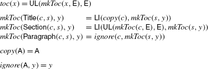
  and horizontally-repeated sequence representing (X)HTML fragments like: <ul><li>A</li><li>A</li>…</ul> Here, a fragment <li> x </li> y and <ul> x </ul> y are represented by LI(x,y) and UL(x,y) respectively, the text A is represented by A, and the empty sequence is represented by E.

• The program toc above and vertically-repeated (nested) (X)HTML fragments like <ul><li>…<ul><li>A</li></ul>…</li></ul>

In the experiment, we only focus on estimation of the asymptotic complexity. For example, we do not focus on the overhead from manually-written inverse programs or the preprocessing cost.

Figure 4 shows the log-log plot of the experimental results. In a log-log plot, a function y=cx ^b is plotted as a straight line, because y=cx ^b implies logy=blogx+logc. To show the estimated asymptotic complexity orders of the inverse computations, we also plotted an additional line in each plot. Note that these additional line are not obtained by fitting; they are added manually just to show how steeply the running time increases.

Fig. 4

Experimental results for reverse, mirror, eval, and toc for two kinds of outputs

In the following, we discuss the experimental results one by one. Throughout the discussions, we use n for the size of the original output tree fed to the inverse computation that we focus on.

5.2.1 reverse

The running time of the inverse computation for reverse is estimated as O(n ²) from Fig. 4. One might think that this result is strange because we know that the inverse of reverse is reverse and thus can be executed in linear time. This gap comes from the two points: the construction of the tree automaton and the second-order pattern matching.

Regarding the construction of the automaton described in Sect. 4.3, we just used a pair $(\overline {f}, \overline {K})$ to represents a state $q_{ {\langle \overline {f} \rangle }^{-1}(\overline {K})}$ in the automaton. Since in the construction we check if the transitions that go to a state are already generated or not and we used a balanced search tree⁷ for the check, the checks takes O(|q|log|q|) for $q = (\overline {f}, \overline {K})$. For reverse, since the constructed automaton contains O(n) states and each state has the size O(n), the construction itself takes O(n ²logn).

In construction of the transitions of each state, we solve the following second-order matching problems.

$$k[ \mathsf {Cons} (k', \mathsf {Nil} )] \stackrel {?}{=}t \quad \mbox{and} \quad k[ \mathsf {Cons} (k',{\bullet })] \stackrel {?}{=}K $$

Here, we abuse the notation to use $\stackrel {?}{=}$ for the second-order matching problems. The implemented algorithm takes O(n) time to find the solutions, because it searches / from the top of t/K. Thus, since we solve similar second-order matching problems for each state, the cost that comes from the second-order matching is O(n ²).

One might notice that the experiment indicates that the time cost of inverse computation of O(n ²) while the above discussion indicates that it is O(n ²logn). Note that it is hard to observe the difference by logn because the factor is too small for the problem size. Thus, this is not a contradiction.

5.2.2 mirror

The running time of the inverse computation of mirror is estimated as O(n ³) from Fig. 4. Note that the generated automaton contains O(n ²) states because we do not know which part of the list is generated by app or rev. The constructed automaton contains states of the form $q_{ {\langle \mathit {app} , \mathit {rev} \rangle }^{-1}(K^{l-k},K^{m-k})}$ where l+m is equal to the length of an output list (thus, l+m=(n−1)/2) and k≤l,k≤m, and K ⁱ denotes the context of the form of Cons(Z,Cons(Z,…,Cons(Z,•)…)) containing i occurrences of Zs.

The effects of the automaton construction and the second-order matching are similar to those of reverse; the automaton construction and the second-order matching take O(nlogn) and O(n) time for each state, respectively.

5.3 eval

The inverse computation of eval is estimated to run in time O(n ³) from Fig. 4. The constructed automaton contains O(n) states and O(n ²) transition rules.

In contrast to reverse and mirror, the implemented second-order pattern matching takes O(n ²) time for each state. The matching $k[k[{\bullet }]] \stackrel {?}{=}K$ takes O(|K|²) time; the implemented algorithm guesses K ₁ such that K ₁[K ₂]=K, in which there are |K| candidates of such K ₁, and then checks K ₁=K ₂, which takes O(|K|) time. The matching $k_{1}[k_{2}[{\bullet }]] \stackrel {?}{=}K$ also takes O(|K|²) time; the algorithm guesses K ₁ such that K ₁[K ₂]=K (similarly, there are |K| candidates of such K ₁) and takes O(|K|) to check K ₂ has the form k ₂[•].

5.4 toc

From Fig. 4, the estimated complexity of the inverse computation of toc depends on what kind of trees we give to the inverse computation. The constructed automaton contains O(n) states and O(n ²) transitions for horizontally-repeated outputs, and contains O(n ²) states and O(n ³) transitions for vertically-repeated outputs. Note that the program of toc is converted to the following context-generating program.

In horizontally-repeated outputs, which has the form t=UL(LI(A,LI(A,…,LI(A,E)…)),E), there are at most one k such that UL(k[E],E)=t, while, in a vertically repeated outputs, which has the form t=UL(LI(…UL(LI(A,E),E)…,E),E), there are n candidates of k such that UL(k[E],E)=t. This difference causes the difference in the number of states.

The second-order matching took O(n ²) time for each state because we solve $k_{1}[k_{2}[{\bullet }]] \stackrel {?}{=}K$ which takes O(|K|²) time, similar to that in eval.

5.5 Discussions

In this section, we discuss how we can improve the asymptotic complexity of the implemented algorithm. Again, we use n for the size of an output tree that we focus on.

5.5.1 Pointer-representation of contexts

The prototype implementation uses very naive representation of contexts, i.e., a tree with holes, which takes O(n) space and the check of the equivalence also takes O(n) time. Due to this cost, the running time of the inverse computation is usually no better than O(n|Q|) where |Q| is the number of states in the constructed automaton. For example, even for nat in Example 1, the inverse computation takes O(n ²) time, in which the second-order matching $S(k) \stackrel {?}{=}t$—this is nothing but a first-order matching—can be solved in O(1).

A possible solution to the problem is to represent a m-hole context by (m+1) pointers (1 for its root and m for its holes). Since a pointer to the output tree t can be expressed in O(logn) space rather than n, it is expected that the representation reduces the cost of introduction of a state of a constructing automaton. Actually, this representation, combined with the “jumping” technique that will be discussed in Sect. 5.5.2, reduces the cost of the inverse computation for nat, reverse, while it may increase the cost in some cases as described later.

The procedure for the second-order pattern matching is changed according to the change of the representation of contexts. Note that we can see a pointer of an output tree as a state of an automaton representing the output tree. For example, a tree S(S(Z)) can be expressed as an automaton below and each state of the automaton is essentially a pointer of the tree (here we subscript each state by the path from the root).

$$o_{\varepsilon } \leftarrow \mathsf {S} (o_{1}) \qquad o_{1} \leftarrow \mathsf {S} (o_{11}) \qquad o_{11} \leftarrow \mathsf {Z} $$

Then, a context represented by pointers o ₀,o ₁,…,o _m where o ₀ represents its root becomes a type o ₁→…→o _m →o ₀, and the second-order matching problem $e \stackrel {?}{=}K$ becomes the typing problem—finding all the type environment Γ such that Γ⊢e::τ where τ is a pointer representation of K—in the intersection type system used by Kobayashi [29] with an additional restriction that Γ can have multiple entries of k like k::τ ₁,k::τ ₂∈Γ only if τ ₁ and τ ₂ represent the same context. Note that the intersection types do not appear explicitly here because we only consider linear contexts. For example, for e=k ₁[k ₂[Z]] and τ=o _ε in the automaton above, we find the three solutions , and , and for e=k[k[Z]] and the same τ, we find only one solution , which denotes k is used twice to generate the original output tree where one is used to generate a context used to generate a tree at o _ε substituting a tree at o ₁ to its hole and the other is used to generate a context used to generate a tree at o ₁ substituting a tree at o ₁₁ to its hole, and these two contexts are the same. Again, the number of the solutions Γ is bounded by a polynomial of the number of the contexts, and thus a polynomial of n. Note that in the above example we can discard either one of k::o ₁→o _ε and k::o ₁₁→o ₁ because they represent the same context.

With this pointer representation, the inverse computation for nat runs in time O(n). To reduce the cost from O(n) to O(1), we have to know that nat is the identity function on natural numbers and is surjective, which is an orthogonal story to the discussions in this paper.

Note that there is a trade-off between this representation and the naive representation: a context can have n pointer-representations at worst. Thus, although this representation works effectively for reverse, mirror and toc, the constructed automaton for eval now has O(n ²) states and O(n ³) transitions in the pointer representation. Recall that it has O(n) states and O(n ²) transitions in the naive context representation. In the pointer representation, the same contexts S(•) occurring in different positions are distinguished.

5.5.2 Jumping to arbitrary subtrees

As described above, the pointer representation is sometimes useful to reduce the cost of the automaton construction. However, to reduce the cost of the inverse computation, we have to reduce the cost of the second-order matching.

The pointer representation also sheds light on the problem, which enables us to traverse a tree or context from a leaf or arbitrary positions, while we have to traverse a tree or context from a top in the naive representation. For example, for reverse in which we solve the second-order matching problem $k_{1}[ \mathsf {Cons} (k_{2},{\bullet })] \stackrel {?}{=}t$, we have to search Cons(k ₂,•) in t from the top in the naive representation. In contrast, in the pointer representation, the corresponding problem Γ⊢k ₁[Cons(k ₂,•)]::o′→o can be solved in constant time because we can “jump” to the hole position by searching transition rule o″←Cons(o‴,o′).

Finding a good strategy for typing would lead to an efficient second-order matching. Assuming some strategies such as performing “jumping” as possible, we can find that the inverse computation for reverse runs in time O(n) and that for mirror runs in time O(n ²). On the other hand, this technique does not reduce the inverse computation cost for eval.

5.5.3 Special treatment for monadic trees

More optimization can be applicable when the outputs are monadic trees, i.e., trees built only from unary and nullary constructors such as S(S(Z)) and A(B(A(E))). For monadic trees we can use integers for pointers.

Sometimes this integer-representation is useful to solve the second-order matching more efficiently. Consider the second-order matching $k[k[{\bullet }]] \stackrel {?}{=} \mathsf {S} ^{n}({\bullet })$, which, in the integer-representation, can be translated to a problem that enumerating Γ such that Γ⊢k[k[•]]::n→0 where n represents a pointer to the subtree occurring at depth n, or the subtree accessible from the root by a path with length n. Since the pattern is k[k[•]], we know that k splits the context n→0 in the middle. That is, n must be even and . Thanks to the integer representation, we can find this unique candidate of k without investigating the context S ⁿ(•) at all; unlike the pointer representation, we can divide or multiply a “pointer” by a constant in the integer representation. Note that we still have to check if the types n/2→0 and n→n/2 represent the same context or not. The cost of the second-order matching is reduced from O(n ²) to O(n).

In general, for a second-order matching problem $e \stackrel {?}{=}K$, with the integer representation of contexts, we can represent constraints on “shape”s of the free variables in e by linear equations and inequalities. For example, from , we obtain a constraint on shape as x ₁=x ₅∧x ₂=x ₄∧x ₃=x ₀∧(x ₃−x ₂)=(x ₁−x ₀)∧x ₀≤x ₁∧x ₂≤x ₃∧x ₄≤x ₅. Solving the constraint for x ₀,x ₁,x ₂,x ₃, we get x ₁=x ₅,x ₂=x ₄,2x ₀=2x ₃=x ₄+x ₅. By using the technique, the cost of the second-order matching in the inverse computation of eval becomes O(n), and thus the cost of the inverse computation of eval becomes O(n ³) again. This kind of technique is also applicable to list-generating programs like reverse and mirror, and functions of which outputs are partly monadic.

The similar optimization technique has been discussed also in the context of parsing of range concatenation grammars [7] in which users can represent arbitrary number of repetitions of a string. By using the technique, their parsing algorithm accepts 2ⁿ repetitions of a, i.e., $\mathtt{a}^{2^{n}}$, in O(2ⁿ) time.

A much more specialized representation of contexts is applicable for natural numbers represented by S and Z, i.e., trees built from one unary constructor and one nullary constructor. In this situation, we can represent a context by one natural number; for example, we can represents a context S(S(•)) by 2. For eval, since there are no more redundant states in the representation and we can also apply the above optimization techniques to this representation, the inverse computation of eval runs in O(n ²) time in this representation.

5.5.4 Estimation of shape

In the second-order matching, we have not used the fact that a variable k represents a return value of a function. Sometimes, we can perform for efficient inverse computation by using this information.

Consider the following rule of mkToc _c, which is one of the auxiliary functions used by toc _c.

$$\mathit {mkToc} _{\mathrm {c}}( \mathsf {Paragraph} (c,s)) = k_1[k_2[{\bullet }]] ~\mathbf {where}~k_1 = \mathit {ignore} _{\mathrm {c}}(c),k_2 = \mathit {mkToc} _{\mathrm {c}}(s) $$

According to this rule, the inverse computation of toc solves the second-order matching $k_{1}[k_{2}[{\bullet }]] \stackrel {?}{=}K$, which has as many solutions as the size of the context K. However, by using the fact that k ₁ represents a return value of ignore, we know that k ₁ must be •. Combining the fact with other techniques described above, we can solve the second-order matching in constant time.

Exploiting this kind of information, we can achieve the linear time inverse computation for mirror. Recall that, even by using pointer representation, the inverse computation of mirror takes O(n ²) time because the constructed tree automaton contains O(n ²) states. This O(n ²) numbers of states come form the rule

According to the rule, the inverse computation of mirror solves the second-order matching $k_{1}[k_{2}[ \mathsf {Nil} ]] \stackrel {?}{=}t$, which has as many solutions as the size of the output tree t, i.e., O(n) solutions. This is problematic because the inverse computation of each result takes O(n) time, and the most of them produce no answers but introduce O(n) states to the automaton. By using the information that app and rev generate the contexts of the same size, we can know that there is at most one solution for the matching, which makes the time complexity of the inverse computation of mirror be O(n).

It would be a good future direction to discuss how can we estimate the shape and how can we use the estimated shape.

6 Extensions

We shall discuss four extensions of the inverse computation.

6.1 Pattern guards

Sometimes it is useful to define a function with pattern guards. For example, let us consider extending the simple arithmetic-expression language shown in Sect. 1 to include a conditional expression that branches by checking if a number is even or odd:

$$\mathbf {data}~ \mathit {Exp} = \dots \mid \mathsf {CaseParity} ( \mathit {Exp} , \mathit {Exp} , \mathit {Exp} ) $$

According to the change, eval can also be naturally extended by using pattern guards:

Here, we have omitted the definition of even/odd that evaluates n and checks if the result is even/odd or not. We shall not discuss how they are defined at this point.

This extension can be achieved by using the known notion of MTT called look-ahead [15]. With regular look-ahead, we can test an input by using a tree automaton before we choose a rule. For example, even and odd can be seen as look-ahead because they can be expressed by the following tree automaton.

Some pattern guards can be expressed by using regular look-ahead.

To handle regular look-ahead, we have to change the inverse computation method a bit. Consider a rule of the form,

$$f(x) \mid q(x) = g(x). $$

What transition rule should we produce from this f and a given K? Producing a rule $q_{f^{-1}(K)} \leftarrow q_{g^{-1}(K)}$ as the method discussed in Sect. 4.3 is unsatisfactory because the rule f(x)∣q(x)=g(x) is applicable only if x is accepted in q. Thus, we must embed the look-ahead information in the transition rule. This embedding can be naturally expressed by using an alternating tree automaton [10]:

$$q_{f^{-1}(K)} \leftarrow q_{g^{-1}(K)} \wedge q $$

However, using an alternating tree automaton does not fit our purpose because extracting a tree from an alternating tree automaton takes at worst time exponential to the size of the alternating tree automaton [10]; thus, it is difficult to bound the cost of our inverse computation polynomially to the original output size. Moreover, it also reduces the simplicity of the inverse computation method.

To keep our inverse computation method simple, we can specialize [35] the functions in a program to look-ahead as a preprocess. In a specialized program, for any function call $g(x,\overline {e})$ in a rule $f(p,\dots) \mid \dots q(x) \dots = \dots g(x,\overline {e}) \dots$, the domain of the function must be accepted by the look-ahead; i.e., ${\mathopen {[\![}g\mathclose {]\!]}}(s,\overline {t}) = t$ implies s∈[[q]]. Thus, in a specialized program, look-ahead cannot affect the inverse computation results (recall that programs are assumed to be nondeleting). For example, the specialized version of evalAcc is

Recall that we use ignore because of the restriction that a program must use every input variable at least once. The functions ignore _e and ignore _o are specialized versions of ignore (to even and odd respectively):

Here, we have omitted most of the definition of ignore _o . The above program has been simplified by using the fact that every input is either even or odd.

The specialization of a program increases the program size [33, 35]. In the worst case, a specialized program is |Q|^N times as big as the original one and the specialization takes time proportional to the size of the specialized program, assuming that look-ahead is defined by a deterministic [10] tree automaton with the states Q, where N is the maximum arity of the constructors. Since this only increases the program size, our method still runs in time polynomial to the size of the original output.

6.2 Bounded use of parameters

The notion of look-ahead can relax the parameter-linearity restriction to finite-copying-in-parameter [12]. An MTT is called finite-copying-in-parameter [12] if there is a constant b such that K obtained by [[f]](s,•₁,…,• _m )=K uses each hole • _j (1≤j≤m) at most b times for every function f of arity m+1 and s. It is known that every finite-copying-in-parameter MTT can be converted into a parameter-linear MTT with look-ahead (see the proof of Lemma 6.3 in [12]). For example, the following MTT copies a parameter zero times or twice.

$$f(x) = g( x, \mathsf {A} ) \quad g( \mathsf {A} , y) = \mathsf {C} (y,y) \quad g( \mathsf {B} , y) = \mathsf {D} $$

By using look-ahead, we can convert it into a parameter-linear MTT.

Here, g _i means g that copies the output variable i times and q _i means the set of the inputs for which g copies the output variable i times.

We can easily extend the method in Lemma 6.3 of [12] to generate specialized functions. A converted program can be (b+1)^MF(N+1)-times as big as the original one, where b is the bound of the parameter copies, N is the maximum arity of the constructors, F is the number of functions, and M is the maximum arity of the functions.

6.3 Parameter-linear macro forest transducers

A macro forest transducer [41], which is an important extension of a macro tree transducer, generates forests (roughly speaking, sequences of trees) instead of trees, which enables us to express XML transformations and serialization programs more directly. Our polynomial-time inverse computation results can be lifted to parameter-linear macro forest transducers.

Unlike macro tree transducers, in macro forest transducers, we can use the sequence concatenation “⋅” in right-hand sides. The function toc defined below is an example of a macro forest transducer, which makes the table-of-contents of a document:

Here, ε denotes the empty sequence, and copy is defined as copy(σ(x ₁)⋅x ₂)=σ(copy(x ₁))⋅copy(x ₂) for any symbol σ and copy(ε)=ε. For an input Title(A)⋅Section(Title(B)⋅Paragraph(…))⋅Title(C), which represents an XML fragment

toc produces an output UL(LI(A)⋅UL(LI(B))⋅LI(C)), which represents the XML fragment below.

In general, a rule of a (stay) macro forest transducer has the form of either

$$f(\varepsilon ,\overline {y}) = e, \qquad f(\sigma(x_1) \cdot x_2,\overline {y}) = e, \quad \mbox{or} \quad f(x,\overline {y}) = e, $$

where each expression e is defined by the following BNF.

$$e ::= \sigma(e_1) \mid e_1 \cdot e_2 \mid y \mid f(x,e_1,\dots,e_m) $$

A transformation like toc, which does not use accumulation parameters, can be expressed by a macro tree transducer, under some encoding of forests. However, this is not possible in general [41]; in general two macro tree transducers are required: one generates a forest in which the concatenations “⋅” are frozen [47] and the other thaws the frozen concatenations [41]. Thus, an extension is needed if we extend our results to parameter-linear macro forest transducers.

We also can perform polynomial time inverse computation for (deterministic) parameter-linear macro forest transducers. Recall that the following points are the keys to our polynomial-time result.

• 1. We can see a program as a linear non-accumulative context-generating program.

• 2. The number of contexts in a given output is bounded by a polynomial to the size of the output.

• 3. The substitutions of $\overline {e}\varTheta = \overline {K}$ can be enumerated in polynomial time. Since the solution space is bounded polynomially by the second item, the existence of the polynomial-time checking of the equivalence of two contexts is sufficient.

Regarding Item 1, it is rather clear that we can apply the transformations discussed in Sect. 4.1 and Sect. 4.2 for macro forest transducers. Regarding Item 2, the number of m-hole linear contexts in a forest is bounded by O(n ^2m+2) where n is the size of the forest; there are O(n ²) subforests in a forest of size n similarly to the number of substrings in a string, and a linear m-hole context can be seen as a forest in which m subforests are replaced by holes. Item 3 is clear in the standard context representation in which a context is expressed as a forest with special symbols representing holes.

Note that, for linear macro forest transducers, where the uses of the both input and output variables are linear, polynomial-time inverse computation can be performed simply by preprocessing. For a linear macro forest transducer, the size of an output forest is bounded linearly by the size of the input forest, i.e., the transformation is linear size increase [14]. Thus, a linear macro forest transducers is MSO-definable because it is expressed as compositions of MTTs and linear size increase [14]. Since MSO-definable tree transformation can be represented by a MTT that is both finite-copying-in-the-inputs and finite-copying-in-parameter [12], our method becomes applicable with some extra preprocessing as noted in Sect. 6.2.

6.4 Composing with inverse-image computation

Recall that our inverse computation method returns a set of corresponding inputs as a tree automaton. To enlarge the class of functions for which polynomial-time inverse computation can be performed, it is natural to try composing our inverse computation with inverse-image computation—computation of the set for a problem f and a given set of outputs T—which has been studied well in the context of tree transducers (for example, [15, 17, 32]).

However, there are several difficulties on this attempt:

• Usually, the inverse-image computation is harder than P. For example, it is known that the complexity of the inverse-image computation is EXPTIME-complete even for MTTs without output variables, which are thus non-accumulative, when T and the result set are given in tree automata [34].

• A few results are known on polynomial time inverse-image computation. However, some method [17] requires that a set of output trees must be given in a deterministic tree automaton; in general, converting a tree automaton to a deterministic one causes exponential size-blow-up.

• For some programs, polynomial-time inverse-image computation is possible even if we use a non-deterministic tree automaton to represents a set of outputs. However, composing these methods sometimes does not increase the expressive power. For example, although it is not difficult to see that polynomial-time inverse-image computation can be performed for MSO-definable transducers, the composition of a MSO-definable transducer followed by a parameter-linear MTT can also be expressed in a parameter-linear MTT [12].

We have to overcome the problems to enlarge the applicability of our method. Luckily, we can overcome the problems listed above.

• The inverse-image computation method proposed by Frisch and Hosoya [17] runs in polynomial-time for MTTs with the restriction of finite-input-copying-in-the-inputs [12].

• The method requires deterministic tree automata, but the automata obtained by our inverse computation can be converted to deterministic ones in polynomial time; there is no exponential size blow-up.

• The composition of a finite-input-copying-in-the-inputs MTT followed by a parameter-linear MTT can express a transformation that cannot be expressed in a single MTT, although the resulting class is artificial.

The following program multiply, which performs multiplication of two natural numbers, is an example for the third item.

$$\mathit {multiply} (x) = \mathit {sum} ( \mathit {dist} (x)) $$

Here, the function nat is the same as that in reverse and mirror. The function multiply defines a mapping P(S ⁿ(Z),S ^m(Z))↦S ^mn(Z). Note that multiply is defined by a composition of the two functions: the one is sum written in a parameter-linear MTT, the other is dist written in a finite-input-copying-in-the-inputs MTT [12].

In the following, we show that the automata obtained by our inverse computation can be converted to deterministic ones in polynomial time. A tree automaton is called ϵ-free if it contains no rules of the form of q←q′. A tree automaton is called deterministic [10] if it is ϵ-free and its transition rules contain no two different rules q←σ(q ₁,…,q _n ) and q′←σ(q ₁,…,q _n ) for any σ and q ₁,…,q _n . Note that we can convert a automaton to an ϵ-free one in polynomial-time [10].

A key property here is that, in an automaton obtained by our inverse computation, each state has the form $q_{ {\langle \overline {f} \rangle }^{-1}(\overline {K})}$ and it satisfies that $s \in {\mathopen {[\![}q_{ {\langle \overline {f} \rangle }^{-1}(\overline {K})}\mathclose {]\!]}}_{\mathcal{A}_{ \mathrm {I} }}$ if and only if ${\mathopen {[\![} {\langle \overline {f} \rangle } \mathclose {]\!]}}(s) = (\overline {K})$ (Theorem 1). Using the fact, we obtain the following lemma:

Lemma 2

For any $\overline {K}$, $\overline {K'}$, $\overline {f}$ and $\overline {f'}$ satisfying $K_{i} \ne K'_{i}$ and $f_{i} = f'_{i}$ for some i,

$${\mathopen {[\![}q_{ {\langle \overline {f} \rangle }^{-1}(\overline {K})}\mathclose {]\!]}}_{\mathcal{A}_ \mathrm {I} } \cap {\mathopen {[\![}q_{ {\langle \overline {f'} \rangle }^{-1}(\overline {K'})}\mathclose {]\!]}}_{\mathcal{A}_ \mathrm {I} } = \emptyset $$

holds.

Proof

We prove the lemma by contradiction. Suppose that we have ${\mathopen {[\![}q_{ {\langle \overline {f} \rangle }^{-1}(\overline {K})}\mathclose {]\!]}}_{\mathcal{A}_{ \mathrm {I} }} \cap {\mathopen {[\![}q_{ {\langle \overline {f'} \rangle }^{-1}(\overline {K'})}\mathclose {]\!]}}_{\mathcal{A}_{ \mathrm {I} }} \ne \emptyset$ for some $\overline {f}$, $\overline {f}'$, $\overline {K}$ and $\overline {K'}$ such that $f_{i} = f'_{i}$ and $K_{i} \ne K_{i}'$ for some i. According to Theorem 1, there exists some s such that ${\mathopen {[\![} {\langle \overline {f} \rangle } \mathclose {]\!]}}(s) = \overline {K}$ and ${\mathopen {[\![} {\langle \overline {f}' \rangle } \mathclose {]\!]}}(s) = \overline {K'}$. That is [[f _i ]](s)=K _i and ${\mathopen {[\![}f'_{i}\mathclose {]\!]}}(s) = K'_{i}$. Since $f_{i} = f_{i}'$ and [[f _i ]] is a function because we consider deterministic MTTs, we have $K_{i} = K'_{i}$, which contradicts the assumption $K_{i} \ne K'_{i}$. □

The lemma guarantees that the naive subset-construction [10], which converts a tree automaton to a deterministic one, runs in polynomial-time. In the subset-construction, we construct an automaton whose states are represented by sets of states of the input automaton. A key property is that, in the constructed automaton, every state accepts at least one tree. Thus, if we apply the subset construction to the resulting automaton of our inverse computation, each state P in the generated automaton does not contain two states $q_{ {\langle \overline {f} \rangle }^{-1}(\overline {K})}$ and $q_{ {\langle \overline {f'} \rangle }^{-1}(\overline {K'})}$ with $K_{i} \ne K'_{i}$ and $f_{i} = f'_{i}$ in P. Therefore, the number of states in the constructed automaton is bounded by the number of mappings from a function f in the original program to a context K, which is O(n ^FM) where n is the size of an original output fed to the inverse computation, F is the number of functions in the original program and M is the maximum arity of the functions. Note that the number of states in the resulting automaton of our inverse computation is also O(n ^FM) (see the proof of Theorem 2).

Since we can convert an automaton obtained by our inverse computation to a deterministic one in polynomial-time, we can perform polynomial-time inverse computation for a transformation that is defined by a finite-copying-in-the-inputs MTT followed by a finite-copying-in-parameter MTT.

Note that the class of the transformations defined by a finite-copying-in-the-inputs MTT followed by a finite-copying-in-parameter MTT is incomparable with that defined by a MTT. In MTT, we can write a transformation that increases the size of a tree double-exponentially as below

while we cannot express such a transformation in the class of the transformations defined by a finite-copying-in-the-inputs MTT followed by a finite-copying-in-parameter MTT. For a finite-copying-in-the-inputs MTT, it is not difficult to show that the height of an output tree is bounded linearly by the size of the input tree, and for a parameter-linear MTT (with look-ahead), it is known that the size of an output tree is bounded exponentially by the height of the input tree [47]. Thus, for the class of the composed transformations, the size of an output tree is bounded exponentially by the size of the input tree, which excludes dexp.

7 Related work

7.1 Inverse computation

There have  been  many  studies  on  the  inverse  computation  problem [1, 20, 21, 23, 30, 37, 40, 49]. They can be categorized into those on left-inverse computation and those on right-inverse computation. Left-inverse computation [20, 21, 23, 30, 40] focuses on injective functions and tries to make an efficient inverse computation based on injectivity analysis, but it can only handle provably-injective functions. Right-inverse computation [1, 37, 49] including ours can handle more functions than left-inverse computation does—it works even for non-injective functions—but the yielded inverse-computation process is usually much slower than that of left-inverse computation. Another important difference is that left-inverse computation is compositional; if we have effective left-inverse computation methods for f and g, we have an effective left-inverse computation method for f∘g. On the other hand, right-inverse computation may not be compositional; even if we have right-inverse computation methods for f and g, then right-inverse computation may happen to be undecidable for f∘g. Left-inverse computation is suitable for applications in which efficiency is the biggest concern, such as in serialization/deserialization. On the other hand, right-inverse computation is suitable for applications in which one wants to invert non-injective function to enumerate all the corresponding inputs, such as in test-case generation [9, 43]. It is worth noting that checking the injectivity of a function is generally undecidable. For parameter-linear MTTs in particular, the injectivity check is undecidable even if it has no output-variables [18] or it has no multiple data traversals (we can reduce the ambiguity check of a context-free grammar, which is known to be undecidable [24], to the problem). Thus, any left-inverse computation method essentially has a function written in parameter-linear MTT that cannot be inverted by it.

To the best of our knowledge, there are few discussions on the topic of multiple data traversals, except for Eppstein’s work [16]. He demonstrated the usefulness of tupling [8, 25] that can make an injective function from non-injective functions.

Regarding accumulations, studies on left-inverse computation have treated them heuristically [20, 39, 40] because the injectivity check is usually undecidable with them. Glück and Kawabe [20] use the LR-parsing technique. In their system, if the grammar obtained from a program is LR-parsable, inverse program based on LR-parsing is derived. Note that their use of grammar is different from our use of tree automaton: their grammar represents a set of possible instruction sequences (traces) of a program while our tree automaton represents a set of inverse computation results. Nishida and Vidal [40] and Mogensen [39] focus on the special tail-recursive (thus usually accumulative) pattern and discuss the inverse computation of the pattern. Regarding right-inverse computation, although there are few studies focusing on accumulative functions, the approaches [17, 32] regarding the inverse-image computation have a strong connection to this work and will be discussed later in this section.

7.2 Results on tree transducers

We assumed that the programs are deterministic and showed that a tractable inverse computation is possible for parameter-linear MTTs. However, this result does not scale to nondeterministic programs. Even for MTTs without output variables, the problem of checking whether an inverse-computation result is empty or not is known to be NP-complete [42]. This means the complexity of the inverse computation problem of the nondeterministic MTTs even without output variables is NP-hard. For compositions of (deterministic/nondeterministic) macro tree transducers, checking whether an inverse-computation result is empty or not is known to be in NP [28]; thus the problem is NP-complete for compositions of nondeterministic macro tree transducers. It is still open whether the problem is NP-hard or not for compositions of deterministic macro tree transducers.

The problem of inverse computation takes a function f and an output tree t and returns the trees s such that f(s)=t. A similar problem, the inverse-image computation problem—computation of the set for a given f and T—has been studied on tree transducers (for example, [15, 17, 32]). The difference from the inverse computation problem is that the inverse computation takes one tree but inverse-image computation takes a set of trees, and this difference is a key to our polynomial-time result. The complexity of the inverse-image computation is EXPTIME-complete even for the parameter-linear MTTs without output variables which are thus non-accumulative, when T and the result set are given in tree automata [34]. Roughly speaking, their EXPTIME-hard result is caused by intersections; for an expression like …f(x)…f(x)… we essentially have to compute the intersection in the inverse-image computation [34]. On the other hand in our method, we do not need to compute the intersection because, for trees t ₁ and t ₂, equals if t ₁=t ₂, and otherwise it is empty. This is implicitly expressed by the transformation in Sect. 4.1, in which we replace …f(x)…f(x)… by …k…k… where k=f(x); a multiple data traversal is replaced by an output copying.

The observation that an MTT program is a non-accumulative context-generating transformation plays an important role in our method. A similar but different idea is exploited in inverse-image computation [17, 32]. Unlike our approach, the idea is to view an MTT program as a non-accumulative mapping-generating transformation, where a mapping is represented by input-output pairs. A context is different from a mapping; it contains more information than a mapping, e.g., the information about the positions of holes. This difference results in the difference in inverse computation between our context-generation view and the mapping-generation view. The mapping-generation view considers mappings from a tuple of subtrees of t to a subtree of t for the original output t, which are indeed partially-applied functions such as $\lambda \overline {y}.{\mathopen {[\![}f\mathclose {]\!]}}(s,\overline {y})$ used to generate t. However, the number of m-ary mappings on the subtrees of t is exponential to the size of t [17, 32]. Although the inverse computation based on the mapping-generation view can be performed in polynomial-time if there are no multiple data traversals [17], it is unclear whether polynomial-time inverse computation for functions with multiple-data traversals can be achieved or not. In contrast, we exploit the linearity of the holes—a context contains this information but a mapping does not—to achieve polynomial-time inverse computation for parameter-linear MTTs, in which a function can have multiple data traversals. Note that, like m-ary functions, the number of non-linear m-hole subcontexts in a tree is bounded exponentially by the size of the tree, whereas the number of linear ones is bounded polynomially by the size.

Regarding inverse computation of general MTTs, there is another polynomial-time inverse computation method besides ours that works for a subset of MTTs. The method of [17], as mentioned in the previous paragraph, runs in polynomial time for MTTs without multiple data traversals, i.e., MTTs with the restriction of finite-input-copying-in-the-inputs [12]. In the restricted class of MTTs, we can copy an output unboundedly many times but we can traverse an input in only a bounded number of times. For example, reverse and mirror are finite-copying-in-the-inputs, but eval is not. In contrast, our method runs in polynomial time for (deterministic) MTTs with the restriction of finite-copying-in-the-output (Sect. 6.2), in which we can traverse an input unboundedly many times but we can copy an output only a bounded number of times. Whether we can perform polynomial-time inverse computation for general deterministic MTTs or not is still an open problem. It is worth noting that many useful functions can be written as an MTT in which both the input traversals and the output copies are bounded [12–14, 32], and thus inverse computation for the functions can be performed in polynomial time both by theirs and ours. Thus, the difference in expressiveness between ours and other methods is rather small, though not negligible. However, we claim that our method stands out by being systematic and simple.

7.3 (Formal) Grammars

In previous work [37], we have suggested an idea for inverse computation: We first find a grammar representing the possible outputs of a program, and then perform inverse computation through the parsing of the grammar. For left-inverse computation, we use an unambiguous grammar that over-approximates the possible outputs of a program, and for right-inverse computation, we use a grammar that exactly represents the possible outputs of a program but the grammar need not to be unambiguous. In [37], we have mainly discussed inverse computation using regular tree grammars [10], and showed that linear-time (right-)inverse computation is possible for affine and treeless [48] programs. For some subclass of MTTs, we can achieve polynomial-time inverse computation via parsing; for example, we can use context-free tree grammars for linear macro tree transducers and we can use IO macro grammars [5] for input-linear MTTs. However, to the best of our knowledge, there is no (tree) grammar that is powerful enough to express the possible outputs (range) of parameter-linear MTTs and is parsable in polynomial time.

However, this paper borrows the ideas from formal grammars in inverse computation. In this sense this work is also “grammar-based” as our previous work [37]. Concretely, we borrow the idea from the parsing algorithm of range concatenation grammars (RCG) [7]. RCG can mimic the ranges of some parameter-linear MTTs. Note that the following program exp, which is a simplified version of ev and eval, is a typical example of transformations that cannot be handled by the existing inverse computation methods

We focus on RCG because it can express the possible outputs of exp and there is polynomial-time parsing algorithm. In RCG, we define a grammar by using Horn clauses as follows.

This grammar expresses a set of strings $\{ \mathtt{a}^{2^{n}} \mid n \in \mathbb{N} \}$. One might notice that the first rule of this grammar has a similar structure to the inverse computation for the rule of ex _c for Dbl

$$\mathit {ex} ( \mathsf {Dbl} (x)) = k[k[{\bullet }]] ~\mathbf {where}~ k = \mathit {ex} (x) $$

where ex ⁻¹(K) try to find K′ such that K=K′[K′[•]] and then try to compute ex ⁻¹(K′). Only the difference is that RCG uses eq explicitly in some reason. (Note that this use of eq is mandatory in RCG because variables such as X and Y ranges over occurrences of strings (called ranges in [7]) instead of strings themselves, similar to the pointer-representation discussed in Sect. 5.5.1. But, this difference is ignorable if we do not use the same variable twice in the left-hand sides and do not allow concatenations in the right-hand sides.) In RCG, polynomial-time parsing is performed by range-wise memoization. We follow the idea and achieve the polynomial-time inverse computation by context-wise memoization.

One would notice that the idea of the parsing with range-wise memoization is already used Cocke-Younger-Kasami (CYK) parsing [24] for context-free grammars. Indeed, both of the parsing algorithm of RCG and our inverse computation method are extensions of CYK parsing. We can see a context-free grammar as a transformation from a concrete syntax tree to the corresponding string, and we can write the transformation by a parameter-linear MTT. Then, our inverse computation for the transformation behaves as CYK parsing for the grammar, although the time complexity of the inverse computation depends on what second-order matching algorithm we use.

It is known that RCG is P-complete, i.e., RCG can express any set of strings of which membership test is performed in polynomial-time [7]. However, we have not used the full-expressive power of RCG. Filling this gap is a future direction.

8 Conclusion

We have shown that viewing a function as a context-generating transformation simplifies inverse computation of accumulative functions with multiple data traversals. Accordingly, we can achieve systematic polynomial-time inverse computation with small modifications to the existing techniques.

A future direction is to develop a systematic program inversion method for accumulative functions based on the view point. Since now an accumulative function can be viewed as non-accumulative context-generating functions, we hope that we can extend usual range-analysis-based program-inversion methods [21, 30, 37] to those functions, and hope that a program-inversion method developed in this way would be a good alternative to the existing approaches [20, 39, 40]. Another future direction is to develop an inverse computation method that can handle more kinds of copying. One sort of the interesting copying in practice is those introduced by “join” operation in database query. Although this study is the first one to tackle the problem of “copies” in inverse computation, still there is a large gap between our results and the general “join” functions used in practice. Since tree transducers are hardly able to express “join”-like transformation [38], the next step in our research would be to identify what “join”s we should treat by designing an appropriate language.

References

Abramov, S.M., Glück, R.: Principles of inverse computation and the universal resolving algorithm. In: Mogensen, T.Æ., Schmidt, D.A., Sudborough, I.H. (eds.) The Essence of Computation. Lecture Notes in Computer Science, vol. 2566, pp. 269–295. Springer, Berlin (2002)
Abramov, S.M., Glück, R., Klimov, Y.A.: An universal resolving algorithm for inverse computation of lazy languages. In: Virbitskaite and Voronkov [46], pp. 27–40
Albert, E., Vidal, G.: The narrowing-driven approach to functional logic program specialization. New Gener. Comput. 20(1), 3–26 (2001)
Antoy, S., Echahed, R., Hanus, M.: A needed narrowing strategy. J. ACM 47(4), 776–822 (2000)
Asveld, P.R.: Time and space complexity of inside-out macro languages. Int. J. Comput. Math. 10(1), 3–14 (1981)
Bird, R.: Introduction to Functional Programming Using Haskell, 2nd edn. Prentice Hall, New York (1998)
Boullier, P.: Range concatenation grammars. In: Bunt, H., Carroll, J., Satta, G. (eds.) New Developments in Parsing Technology. Text, Speech and Language Technology, vol. 23. Kluwer Academic, Dordrecht (2004). Chap. 13
Chin, W.-N., Khoo, S.-C., Jones, N.: Redundant call elimination via tupling. Fundam. Inform. 69(1–2), 1–37 (2006)
Christiansen, J., Fischer, S.: EasyCheck—test data for free. In: Garrigue, J., Hermenegildo, M.V. (eds.) FLOPS. Lecture Notes in Computer Science, vol. 4989, pp. 322–336. Springer, Berlin (2008)
Comon, H., Dauchet, M., Gilleron, R., Löding, C., Jacquemard, F., Lugiez, D., Tison, S., Tommasi, M.: Tree automata techniques and applications (2007). http://www.grappa.univ-lille3.fr/tata
Dowek, G.: A second-order pattern matching algorithm for the cube of typed lambda-calculi. In: MFCS, pp. 151–160 (1991)
Engelfriet, J., Maneth, S.: Macro tree transducers, attribute grammars, and MSO definable tree translations. Inf. Comput. 154(1), 34–91 (1999)
Engelfriet, J., Maneth, S.: A comparison of pebble tree transducers with macro tree transducers. Acta Inform. 39(9), 613–698 (2003)
Engelfriet, J., Maneth, S.: Macro tree translations of linear size increase are MSO definable. SIAM J. Comput. 32(4), 950–1006 (2003)
Engelfriet, J., Vogler, H.: Macro tree transducers. J. Comput. Syst. Sci. 31(1), 71–146 (1985)
Eppstein, D.: A heuristic approach to program inversion. In: IJCAI, pp. 219–221 (1985)
Frisch, A., Hosoya, H.: Towards practical typechecking for macro tree transducers. In: Arenas, M., Schwartzbach, M.I. (eds.) DBPL. Lecture Notes in Computer Science, vol. 4797, pp. 246–260. Springer, Berlin (2007). Full version is available as Research Report, RR-6107, INRIA, 2007
Fülöp, Z.: Undecidable properties of deterministic top-down tree transducers. Theor. Comput. Sci. 134(2), 311–328 (1994)
Giesl, J., Kühnemann, A., Voigtländer, J.: Deaccumulation techniques for improving provability. J. Log. Algebr. Program. 71(2), 79–113 (2007)
Glück, R., Kawabe, M.: Derivation of deterministic inverse programs based on LR parsing. In: Kameyama, Y., Stuckey, P.J. (eds.) FLOPS. Lecture Notes in Computer Science, vol. 2998, pp. 291–306. Springer, Berlin (2004)
Glück, R., Kawabe, M.: Revisiting an automatic program inverter for lisp. SIGPLAN Not. 40(5), 8–17 (2005)
Glück, R., Sørensen, M.H.: Partial deduction and driving are equivalent. In: Hermenegildo, M.V., Penjam, J. (eds.) PLILP. Lecture Notes in Computer Science, vol. 844, pp. 165–181. Springer, Berlin (1994)
Gries, D.: The Science of Programming. Springer, Heidelberg (1981). Chap. 21 “Inverting programs”
Hopcroft, J.E., Motwani, R., Ullman, J.D.: Introduction to Automata Theory, Languages, and Computation, 3rd edn. Prentice Hall, New York (2006). Chap. 7
Hu, Z., Iwasaki, H., Takeichi, M., Takano, A.: Tupling calculation eliminates multiple data traversals. In: ICFP, pp. 164–175 (1997)
Huet, G.P.: Résolution d’équations dans les langages d’ordre 1,2,…,ω. PhD thesis, Université de Paris VII (1976)
Huet, G.P., Lang, B.: Proving and applying program transformations expressed with second-order patterns. Acta Inform. 11, 31–55 (1978)
Inaba, K., Maneth, S.: The complexity of tree transducer output languages. In: Hariharan, R., Mukund, M., Vinay, V. (eds.) FSTTCS. LIPIcs, vol. 2, pp. 244–255. Schloss Dagstuhl—Leibniz-Zentrum fuer Informatik (2008)
Kobayashi, N.: Types and higher-order recursion schemes for verification of higher-order programs. In: Shao, Z., Pierce, B.C. (eds.) POPL, pp. 416–428. ACM, New York (2009)
Korf, R.E.: Inversion of applicative programs. In: Hayes, P.J. (ed.) IJCAI, pp. 1007–1009. Kaufmann, Los Altos (1981)
Kühnemann, A., Glück, R., Kakehi, K.: Relating accumulative and non-accumulative functional programs. In: Middeldorp, A. (ed.) RTA. Lecture Notes in Computer Science, vol. 2051, pp. 154–168. Springer, Berlin (2001)
Maneth, S., Nakano, K.: XML type checking for macro tree transducers with holes. In: PLAN-X (2008)
Maneth, S., Perst, T., Seidl, H.: Exact XML type checking in polynomial time. In: Schwentick, T., Suciu, D. (eds.) ICDT. Lecture Notes in Computer Science, vol. 4353, pp. 254–268. Springer, Berlin (2007)
Martens, W., Neven, F.: On the complexity of typechecking top-down XML transformations. Theor. Comput. Sci. 336(1), 153–180 (2005)
Matsuda, K., Hu, Z., Takeichi, M.: Type-based specialization of XML transformations. In: Puebla, G., Vidal, G. (eds.) PEPM, pp. 61–72. ACM, New York (2009)
Matsuda, K., Inaba, K., Nakano, K.: Polynomial-time inverse computation for accumulative functions with multiple data traversals. In: Kiselyov, O., Thompson, S. (eds.) PEPM, pp. 5–14. ACM, New York (2012)
Matsuda, K., Mu, S.-C., Hu, Z., Takeichi, M.: A grammar-based approach to invertible programs. In: Gordon, A.D. (ed.) ESOP. Lecture Notes in Computer Science, vol. 6012, pp. 448–467. Springer, Berlin (2010)
Milo, T., Suciu, D., Vianu, V.: Typechecking for XML transformers. J. Comput. Syst. Sci. 66(1), 66–97 (2003)
Mogensen, T.Æ.: Report on an implementation of a semi-inverter. In: Virbitskaite and Voronkov [46], pp. 322–334
Nishida, N., Vidal, G.: Program inversion for tail recursive functions. In: Schmidt-Schauß, M. (ed.) RTA. LIPIcs, vol. 10, pp. 283–298. Schloss Dagstuhl—Leibniz-Zentrum fuer Informatik (2011)
Perst, T., Seidl, H.: Macro forest transducers. Inf. Process. Lett. 89(3), 141–149 (2004)
Rounds, W.C.: Complexity of recognition in intermediate-level languages. In: FOCS, pp. 145–158. IEEE Press, New York (1973)
Runciman, C., Naylor, M., Lindblad, F.: SmallCheck and lazy SmallCheck: automatic exhaustive testing for small values. In: Gill, A. (ed.) Haskell, pp. 37–48. ACM, New York (2008)
Salvati, S., de Groote, P.: On the complexity of higher-order matching in the linear lambda-calculus. In: Nieuwenhuis, R. (ed.) RTA. Lecture Notes in Computer Science, vol. 2706, pp. 234–245. Springer, Berlin (2003)
Turchin, V.F.: The concept of a supercompiler. ACM Trans. Program. Lang. Syst. 8(3), 292–325 (1986)
Virbitskaite, I., Voronkov, A. (eds.) Perspectives of Systems Informatics, 6th International Andrei Ershov Memorial Conference, PSI, Revised Papers, Novosibirsk, Russia, June 27–30, 2006. Lecture Notes in Computer Science, vol. 4378, Springer, Berlin (2007)
Voigtländer, J., Kühnemann, A.: Composition of functions with accumulating parameters. J. Funct. Program. 14(3), 317–363 (2004)
Wadler, P.: Deforestation: transforming programs to eliminate trees. Theor. Comput. Sci. 73(2), 231–248 (1990)
Yellin, D.M.: Attribute Grammar Inversion and Source-to-Source Translation. Lecture Notes in Computer Science, vol. 302. Springer, Berlin (1988)
Acknowledgements
We wish to thank Akimasa Morihata, Meng Wang, and Soichiro Hidaka, who gave us many valuable comments on an earlier version of this work. The discussions in Sect. 5.5.1 are hinted from Naoki Kobayashi and Takeshi Tsukada. We also thank Janis Voigtländer who pointed out the relationship between Sect. 4.1 and deaccumulation. This work was partially supported by Japan Society for the Promotion of Science, Grant-in-Aid for Research Activity Start-up 22800003, when the first author was in Tohoku University, and this work is partially supported by Japan Society for the Promotion of Science, Grant-in-Aid for Young Scientists (B) 24700020.
Author information
Authors and Affiliations
Corresponding author
Additional information
A preliminary summary of this article appeared in Proceedings of PEPM 2012, pp. 5–14, 2012.
Rights and permissions
Open Access This article is distributed under the terms of the Creative Commons Attribution License which permits any use, distribution, and reproduction in any medium, provided the original author(s) and the source are credited.
About this article
Cite this article
Matsuda, K., Inaba, K. & Nakano, K. Polynomial-time inverse computation for accumulative functions with multiple data traversals. Higher-Order Symb Comput 25, 3–38 (2012). https://doi.org/10.1007/s10990-013-9097-8
Published:
Issue Date:
DOI: https://doi.org/10.1007/s10990-013-9097-8