Tensor RG Approach to High-Temperature Fixed Point

Abstract

We study a renormalization group (RG) map for tensor networks that include two-dimensional lattice spin systems such as the Ising model. Numerical studies of such RG maps have been quite successful at reproducing the known critical behavior. In those numerical studies the RG map must be truncated to keep the dimension of the legs of the tensors bounded. Our tensors act on an infinite-dimensional Hilbert space, and our RG map does not involve any truncations. Our RG map has a trivial fixed point which represents the high-temperature fixed point. We prove that if we start with a tensor that is close to this fixed point tensor, then the iterates of the RG map converge in the Hilbert-Schmidt norm to the fixed point tensor. It is important to emphasize that this statement is not true for the simplest tensor network RG map in which one simply contracts four copies of the tensor to define the renormalized tensor. The linearization of this simple RG map about the fixed point is not a contraction due to the presence of so-called CDL tensors. Our work provides a first step towards the important problem of the rigorous study of RG maps for tensor networks in a neighborhood of the critical point.

Appendices

In this paper the expressions “tensor RG” or “tensor network RG” denote the whole circle of ideas of performing RG using tensor networks, not limited to the TRG and TNR algorithms described in this section.

Tensor Representation for the 2D Ising Model

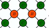
In this appendix we show how to transform the partition function of the nearest-neighbor 2D Ising model on the square lattice with the Hamiltonian $H = -\beta \sum _{\langle i j \rangle } \sigma _i \sigma _j$, $\sigma _i = \pm 1$, to a tensor network built out of 4-tensors as in Fig. 1. We present two ways to perform this transformation.

1.1 Rotated Lattice

This representation was used e.g. in [11]. We start by rotating the spin lattice by 45 degrees. We now associate a tensor with every second square, tensor contractions taking place at the positions of Ising spins:

(A.1)

The Hilbert space has two basis elements $| \sigma \rangle$, $\sigma = \pm$. Assigning tensor components

(A.2)

we reproduce the 2D Ising model partition function. In finite volume this gives the partition function with periodic boundary conditions on the lattice rotated by 45 degrees.

Transforming the basis to the $\mathbb {Z}_2$ even (0) and odd (1) states

(A.3)

the nonzero tensor components become:

$$\begin{aligned} A_{0000} = \cosh (4 \beta ) + 3,\quad A_{0101}=A_{1111} = \cosh (4 \beta ) - 1,\quad A_{0011} = \sinh (4 \beta ), \end{aligned}$$

(A.4)

and rotations thereof. By $\mathbb {Z}_2$ invariance, they all have an even number of 1 indices.

1.2 Unrotated Lattice

Alternatively, one can perform the transformation without rotating the lattice [12, 13]. In finite volume, this method gives the partition function with the usual periodic boundary conditions. We start by representing $W=e^{\beta \sigma _1 \sigma _2}$, viewed as a two-tensor in the Hilbert space with basis elements $| \sigma \rangle$, $\sigma = \pm$, as a contraction of two tensors $W=M M^T$ with

(A.5)

where $c=\cosh \beta$, $s=\sinh \beta$. Graphically

(A.6)

Using 0 and 1 to index the columns of the M matrix, equations

$$\begin{aligned} M_{+0}=M_{-0},\quad M_{+1}=-M_{-1} \end{aligned}$$

(A.7)

mean that the states 0,1 are, respectively, $\mathbb {Z}_2$ even and odd. A tensor network representation of the partition function is obtained by defining

$$\begin{aligned} A_{ijkl}=M_{+i} M_{+j}M_{+k} M_{+l} + M_{-i} M_{-j}M_{-k} M_{-l} \end{aligned}$$

(A.8)

or graphically

(A.9)

The nonzero components are

$$\begin{aligned} A_{0000} = 2 c^2, \quad A_{0011} = A_{0101}=2cs, \quad A_{1111}=2s^2, \end{aligned}$$

(A.10)

and rotations thereof.

1.3 Stability of the High-Temperature Fixed Point

For both representations (A.4) and (A.10), tensor A in the limit $\beta \rightarrow 0$ becomes proportional to the high-temperature fixed point tensor $A_{*}$, as component $A_{0000}$ tends to a constant and all others to zero. Theorem 2.1 allows us to conclude that for sufficiently small temperatures $\beta \leqslant \beta _0$ the tensor RG iterates of A will converge to $A_{*}$.

Exponential Decay of Correlators

The results in this paper do not prove exponential decay of correlation functions when the tensor A is close to the high temperature fixed point. This is not a shortcoming of the tensor network RG approach compared to the Wilson-Kadanoff RG. For the Wilson-Kadanoff RG one can prove that the RG map is rigorously defined and its iterates converge to the trivial fixed point if the starting Hamiltonian is well inside the high temperature phase [3, 4]. However, this by itself does not imply exponential decay of correlations. Of course, if the Hamiltonian is well inside the high temperature phase then standard high temperature expansion methods can be used to prove exponential decay of correlations. Similarly, standard polymer expansion methods can be used to prove exponential decay of correlations for tensor networks when the tensor A is sufficiently close to the high temperature fixed point. We will give a brief sketch of how this is done. This appendix is intended for readers familiar with such techniques, so we will be brief.

We assume that $A=A_*+\delta A$ where $A_*$ denotes the high temperature fixed point as before and $||\delta A||$ is small. We use this equation to expand the partition function (the contraction of the tensor network) into a sum of terms where at each vertex in the lattice there is either $A_*$ or $\delta A$. We call a polymer any connected subset $\gamma$ of lattice sites. The set of lattice sites with $\delta A$ can then be written as the disjoint union of a collection of polymers. The value of this term in the expansion of the partition function is equal to the product of the activities of these polymers where the activity $w(\gamma )$ of a polymer $\gamma$ is the value of the contraction of the tensor network when there is a $\delta A$ at each site in $\gamma$ and an $A_*$ at the sites not in $\gamma$. We then have the bound $|w(\gamma )| \leqslant \Vert \delta A\Vert ^{|\gamma |}$ where $|\gamma |$ is the number of vertices in $\gamma$. Then standard polymer expansion methods can be applied if $\Vert \delta A\Vert \leqslant \epsilon _\mathrm{0}$ [14]. Here $\epsilon _\mathrm{0}$ is some small number which will come out from the standard criteria of the polymer expansion convergence.

Where does tensor RG enter this picture? Our Theorem 2.1 proves that if $\Vert \delta A\Vert \leqslant \epsilon _\mathrm{TRG} =1/C^2$ then we can apply tensor RG repeatedly to make $\Vert \delta A\Vert$ arbitrarily small. We have not worked out in this paper what $\epsilon _\mathrm{TRG}$ or $\epsilon _0$ are. If $\epsilon _\mathrm{TRG}>\epsilon _0$, then the polymer expansion techniques described above cannot be used directly to show that all these tensor networks are in the high-temperature phase. But combining the two we could do this as follows.

In this paper we discussed tensor RG for the partition function. Correlation function can be represented in terms of a tensor network in which some of the A tensors are replaced by other tensors. (The contraction of this network must be divided by the partition function to get the correlation function.) We will refer to these other tensors as B tensors. When one applies tensor RG to the network with some B tensors, these B tensors will be changed as well as the A tensors. We do not have any control over how the norm of the B tensors may change, but that does not matter. After a finite number of iterations of the RG map the tensor A will be sufficienly close to the high temperature fixed point that we can apply a polymer expansion to get exponential decay of the correlation functions.

A calculation of $\epsilon _\mathrm{TRG}$ based directly on the proof in this paper may not give a value greater than $\epsilon _0$. Nonetheless we hope that the value of $\epsilon _\mathrm{TRG}$ can be improved (i.e., increased) considerably by taking advantage of the fact that the tensor RG map happens locally in space. So there is the possibility that the tensor RG can be used to expand the range of temperatures for which we know that the Ising model (and perturbations of it) are in the high temperature phase.

Prior literature on tensor RG

In this paper the expressions “tensor RG” or “tensor network RG” denote the whole circle of ideas of performing RG using tensor networks, not limited to the TRG and TNR algorithms described in this section.

1.1 TRG and Its Variants

Tensor network approach to RG of statistical physics systems was first discussed in 2006 by Levin and Nave [15]. The precise method they introduced, called Tensor RG (TRG), consists in representing tensor A as the product $S S^T$, graphically

(C.1)

and then defining a new tensor by contracting four S tensors:

(C.2)

Decomposition (C.1) is obtained from the singular value decomposition (SVD) $A = U \Lambda U^T$ with $\Lambda$ diagonal and $S = U \sqrt{\Lambda }$. To keep the bond dimension D finite, the singular value decomposition is truncated to the largest D singular values out of the total of $D^2$. Ref.  [15] also defined a similar procedure for the honeycomb lattice. TRG can be used to evaluate numerically the free energy of the 2D Ising model as a function of the temperature and of the external magnetic field on a large finite lattice (reducing it to a one-site lattice by a finite number of TRG steps), and then extract the infinite volume limit by extrapolation. Using bond dimensions up to $D = 34$, Ref.  [15] attained excellent agreement with the exact result except in a small neighborhood of the critical point.

In the introduction we mentioned a simple tensor network RG based on Eq. (1.2), which was also the basis for type I RG step in Sect. 2.2. This procedure was first carried out in [12],¹³ called there HOTRG since it used higher-order SVD in the bond dimension truncation step. More precisely, HOTRG first contracts tensors pairwise in the horizontal direction, and then pairwise in the vertical direction. HOTRG agrees with the exact 2D Ising free energy even better than TRG. Applied to the 3D Ising, it gives results in good agreement with Monte Carlo. The accuracy of TRG and HOTRG is further improved by taking into account the effect of the “environment” to determine the optimal truncation, in methods called SRG [16, 17] and HOSRG [12].

1.2 CDL Tensor Problem

Although TRG and its variants performed very well in numerical free energy computations, it was noticed soon after its inception [18] that the method has a problem. There is a class of tensors describing lattice models with degrees of freedom with ultra-short-range correlators only, which are not coarse-grained away by the TRG method and its above-mentioned variants but passed on to the next RG step unchanged, being exact fixed points of the TRG transformation. These “corner double line” (CDL) tensors (named so in [11]) have a bond space with two indices and the components

$$\begin{aligned} A_{i_1 i_2, j_1 j_2, k_1 k_2, l_1 l_2} = M^{(1)}_{i_1 j_2} M^{(2)}_{j_1 k_1} M^{(3)}_{k_2 l_1} M^{(4)}_{l_2 i_2} \end{aligned}$$

(C.3)

or graphically

(C.4)

with arbitrary matrices $M^{(1)}, \ldots , M^{(4)}$. CDL tensors present a problem both conceptually and practically:

• Conceptually, as we would like to describe every phase by a single fixed point, not by a class of equivalent fixed points differing by a CDL tensor.

• Practically, since every numerical tensor RG computation is performed in a space of finite bond dimension, limited by computational resources. It is a pity to waste a part of this space on uninteresting short-range correlations described by the CDL tensors. This becomes especially acute close to the critical point.

We proceed to discuss algorithms trying to address this problem.

1.3 TEFR

TEFR (tensor entanglement filtering renormalization) was the first algorithm aiming to resolve the problem of CDL tensors [11]. It consists of the following steps:

• 1. Perform SVD to represent A as in Eq. (C.1), truncating to the largest D singular values so that the representation is approximate, where D is the original bond dimension. Tensor S thus has dimension $D \times D \times D$.¹⁴

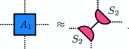
• 2. Find a tensor $S_1$ of dimension $D \times D_1 \times D_1$ with $D_1 < D$ so that¹⁵

  

  (C.5)

  where dashed bonds have dimension $D_1$.

• 3. Recombine tensors $S_1$ to form a four-tensor $A_1$ with dimension $D_1 \times D_1 \times D_1 \times D_1$:

  

  (C.6)

• 4. Perform an SVD to represent $A_1$ along the ”other diagonal”:

  

  (C.7)

• 5. Contract $S_2$ tensors to form tensor $A'_{}$, the final result of the RG step:

  

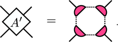  (C.8)

The rationale behind this algorithm is that it reduces an arbitrarily large CDL tensor to a tensor of dimension one in a single RG step [11]. It is less clear what happens for tensors which are not exactly CDL. Ref. [11] gives several procedures for how to perform the key Step 2 for such tensors, but it’s not clear if these are fully successful. Numerical results of [11] for the 2D Ising model are inconclusive. TEFR RG flow converges to the high-temperature fixed point tensor $A_{*}$ for $T > 1.05 T_c$, to the low-temperature fixed point tensor $A_{*} \oplus A_{*}$ for $T < 0.98 T_c$, while in the intermediate range around $T_c$ it converged to a T-dependent tensor with many nonzero components.

Gilt-TNR algorithm (Appendix C.5 below) improves on TEFR by providing a more robust procedure for Step 2.

1.4 TNR

TNR (tensor network renormalization) algorithm by Evenbly and Vidal [2] was perhaps the first method able to address efficiently the CDL tensor problem. It gives excellent results when applied to the 2D Ising model [2], including the critical point. It runs as follows:¹⁶

• 1. Choose a unitary transformation of $V \otimes V$ (“disentangler”). Inserting $u u^{\dagger }$ into the tensor network does not change its value:

  

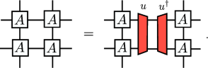  (C.9)

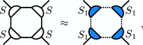
• 2. Choose a couple of isometries $v_1,v_2 : V \rightarrow V \otimes V$. Optimize u, $v_1$, $v_2$ so that

  

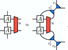  (C.10)

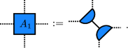
• 3. Rearrange the tensor network as

  

  (C.11)

  where (each blue triangle stands for one of the $v_i$, $v^\dagger _i$ tensors)

  

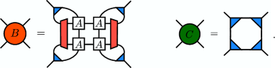  (C.12)

• 4. Perform an (approximate because truncated) SVD for the B and C tensors:

  

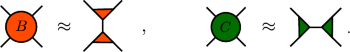  (C.13)

• 5. Finally define the end result of the RG step as

  

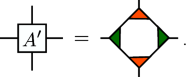  (C.14)

Our type II RG step (Sect. 2.3) was inspired by the TNR algorithm. The main differences and similarities are as follows:

• We work in an infinite-dimensional Hilbert space.

• Our disentanglers R don’t have to be unitary. We insert $R R^{- 1}$ instead of $u u^{\dagger }$.

• We do not choose u and $v_1,v_2$ to minimize the error in (C.10). Rather, our $v_1$, $v_2$ are the identity on $V \otimes V$, while u is chosen to “disentangle” certain correlations between the upper and lower part of TNR B (whose Sect. 2.3 analogue is called S), by killing the $O (\epsilon ^2)$ part of the “dangerous diagram” in (2.39). Since our v’s are the identity, our C is simply a product of Kronecker deltas, realizing a contraction among the indices of B tensors

• Representation $S = S_u S_d$ in (2.35) plays a role similar to the representation of B in (C.13) except that our representation does not involve any truncation and is not required to be an SVD.

• Our Eqs. (2.36) and (2.37) are analogous to the TNR definition (C.14).

Further algorithms aiming to resolve the CDL problem include Loop-TNR [19] and TNR$_+$ [20].

1.5 Gilt-TNR

Gilt(graph independent local truncation)-TNR [13] follows the same steps as TEFR from Appendix C.3. It improves on TEFR by providing a very efficient way to perform Step 2, reducing dimensions of the contraction bonds in the l.h.s. of (C.5) one bond at a time. See [13] for details.

Gilt-TNR is perhaps the simplest tensor network algorithm able to deal with the CDL problem. In addition to the usual 2D Ising benchmarking, Ref.  [13] showed some preliminary results concerning its performance in 3D. It would be interesting to see a computation of the 3D Ising critical exponents by this or any other tensor RG method.

See also [21] for a method combining Gilt with HOTRG from Appendix C.1.

References

Efrati, E., Wang, Z., Kolan, A., Kadanoff, L.P.: Real-space renormalization in statistical mechanics. Rev. Mod. Phys. 86(2), 647–667 (2014). arXiv:1301.6323 [cond-mat.stat-mech]
Evenbly, G., Vidal, G.: Tensor network renormalization. Phys. Rev. Lett. 115(18), 180405 (2015). arXiv:1412.0732 [cond-mat.str-el]
Griffiths, R.B., Pearce, P.A.: Mathematical properties of position-space renormalization-group transformations. J. Stat. Phys. 20(5), 499–545 (1979)
Kashapov, I.A.: Justification of the renormalization-group method. Theor. Math. Phys. 42(2), 184–186 (1980)
Gawedzki, K., Kotecký, R., Kupiainen, A.: Coarse-graining approach to first-order phase transitions. J. Stat. Phys. 47(5), 701–724 (1987)
Bricmont, J., Kupiainen, A.: Phase transition in the 3d random field Ising model. Commun. Math. Phys. 116(4), 539–572 (1988)
van Enter, A.C.D., Fernández, R., Sokal, A.D.: Regularity properties and pathologies of position-space renormalization-group transformations: scope and limitations of Gibbsian theory. J. Stat. Phys. 72(5–6), 879–1167 (1993)
Bricmont, J., Kupiainen, A., Lefevere, R.: Renormalizing the renormalization group pathologies. Phys. Rep. 348(1), 5–31 (2001)
Kennedy, T.: Renormalization group maps for Ising models in lattice-gas variables. J. Stat. Phys. 140(3), 409–426 (2010). arXiv:0905.2601 [math-ph]
Lanford, O.E.: A computer-assisted proof of the Feigenbaum conjectures. Bull. Am. Math. Soc. 6(3), 427–434 (1982)
Gu, Z.-C., Wen, X.-G.: Tensor-entanglement-filtering renormalization approach and symmetry-protected topological order. Phys. Rev. B 80(15), 155131 (2009). arXiv:0903.1069 [cond-mat.str-el]
Xie, Z.Y., Chen, J., Qin, M.P., Zhu, J.W., Yang, L.P., Xiang, T.: Coarse-graining renormalization by higher-order singular value decomposition. Phys. Rev. B 86(4), 045139 (2012). arXiv:1201.1144 [cond-mat.stat-mech]
Hauru, M., Delcamp, C., Mizera, S.: Renormalization of tensor networks using graph independent local truncations. Phys. Rev. B 97(4), 045111 (2018). arXiv:1709.07460 [cond-mat.str-el]
Kotecký, R., Preiss, D.: Cluster expansion for abstract polymer models. Commun. Math. Phys. 103, 491–498 (1986)
Levin, M., Nave, C.P.: Tensor renormalization group approach to 2D classical lattice models. Phys. Rev. Lett. 99(12), 120601 (2007). arXiv:cond-mat/0611687
Xie, Z.Y., Jiang, H.C., Chen, Q.N., Weng, Z.Y., Xiang, T.: Second renormalization of tensor-network states. Phys. Rev. Lett. 103(16), 160601 (2009). arXiv:0809.0182 [cond-mat.str-el]
Zhao, H.H., Xie, Z.Y., Chen, Q.N., Wei, Z.C., Cai, J.W., Xiang, T.: Renormalization of tensor-network states. Phys. Rev. B 81(17), 174411 (2010). arXiv:1002.1405 [cond-mat.str-el]
Levin, M.: Real space renormalization group and the emergence of topological order. Talk at the workshop ‘Topological Quantum Computing. Institute for Pure and Applied Mathematics, UCLA, February 26–March 2 (2007) . http://www.ipam.ucla.edu/abstract/?tid=6595 &pcode=TQC2007
Yang, S., Gu, Z.-C., Wen, X.-G.: Loop optimization for tensor network renormalization. Phys. Rev. Lett. 118(11), arXiv:1512.04938 [cond-mat.str-el] (2017)
Bal, M., Mariën, M., Haegeman, J., Verstraete, F.: Renormalization group flows of Hamiltonians using tensor networks. Phys. Rev. Lett. 118, 250602 (2017). arXiv:1703.00365 [cond-mat.stat-mech]
Lyu, X., Xu, R.G., Kawashima, N.: Scaling dimensions from linearized tensor renormalization group transformations. Phys. Rev. Res. 3(2), 023048 (2021). arXiv:2102.08136 [cond-mat.stat-mech]
Acknowledgements
SR is supported by the Simons Foundation grants 488655 and 733758 (Simons Collaboration on the Nonperturbative Bootstrap), and by Mitsubishi Heavy Industries as an ENS-MHI Chair holder.
Author information
Authors and Affiliations
Corresponding author
Additional information
Communicated by Alessandro Giuliani.
Publisher's Note
Springer Nature remains neutral with regard to jurisdictional claims in published maps and institutional affiliations.