A Compact Treatment of Singular Impurities Using the Artificial Friedel Resonance (FAIR) Technique

Abstract

Building on the tools that Friedel introduced in the 1950s, an off-spring of the Friedel resonance is developed, which is called the FAIR approach for “Friedel Artificially Inserted Resonance”. In the FAIR approach, an arbitrary s-electron state $a_{0}^{\dagger}$ is cut out of the conduction band, and the remaining free electron Hamiltonian is orthogonalized, yielding an artificial Friedel resonance. In the presence of a real Friedel d-resonance state d ^†, one can find an optimal fair state $a_{0}^{\dagger}$ so that the exact n-electron ground state consists of two Slater states, one containing the d-electron and the other the fair state $a_{0}^{\dagger}$. This separation according to the d-occupation is ideal for impurities with a Coulomb interaction between d-electrons. The wave function of the Friedel–Anderson (FA) impurity in the magnetic state and the singlet state are constructed with the FAIR method using two fair states $a_{0}^{\dagger}$ and $b_{0}^{\dagger}$. The magnetic state consists of four, and the singlet state consists of eight Slater states. The latter is invariant with respect to the inversion of all spins. The FAIR ground state Ψ _SS for the singlet state is composed of two magnetic states Ψ _MS with opposite moments which are not orthogonal to each other. The degree of overlap determines the Kondo energy. Because of the compactness of the wave function, a number of properties can be calculated relatively quickly. Comparison with the best previous ground state energy and d-occupation by Gunnarson and Schoenhammer show excellent agreement. A number of physical properties are calculated; among them are (i) the Kondo cloud in a small magnetic field. Two components of polarization are observed (in linear response), an oscillating part and a nonoscillating part. (ii) The fidelity which represents the scalar product between the ground states of the symmetric FA-impurity and the symmetric Friedel impurity is calculated as a function of the number of electron states. (In the literature, this has the somewhat misleading name of fidelity.) This calculation does not show an Anderson orthogonality catastrophe, which indicates that the FA ground state has a phase shift of π/2 at the Fermi energy. (iii) The Friedel oscillations of the FA-impurity. Surprisingly, these oscillations are very similar to the Friedel oscillations of a very narrow Friedel resonance at the Fermi level. The amplitude A(r) is close to zero at short distances and saturates at two for large distances. The inversion point where A(r)=1 correlates with the characteristic energies of the impurities, the half-band width Γ for the Friedel impurity and the Kondo energy for the FA-impurity. This raises the fascinating question how these simple properties are hidden in the multielectron wave function.

Appendices

Appendix A: Wilson’s s-electron Basis

Wilson [10] in his Kondo paper considered an s-band with a constant density of states and the Fermi energy in the center of the band. By measuring the energy from the Fermi level and dividing all energies by the Fermi energy, Wilson obtained a band ranging from −1 to +1. To treat the electrons close to the Fermi level at ζ=0 as accurately as possible he divided the energy interval (−1:0) at energies of −1/Λ,−1/Λ ²,−1/Λ ³,…, i.e., ζ _ν =−1/Λ ^ν. This yields energy cells ℭ _ν with the range {−1/Λ ^ν−1:−1/Λ ^ν} and the width Δ _ν =ζ _ν −ζ _ν−1=1/Λ ^ν. Generally, the value Λ=2 is chosen. (There are equivalent intervals for positive ζ-values where ν is replaced by (N−ν), but we discuss here only the negative energies.) The new Wilson states $c_{\nu}^{\ast}$ are a superposition of all states in the energy interval (ζ _ν−1,ζ _ν ) and have an (averaged) energy $( \zeta_{\nu }+\zeta_{\nu-1} ) /2= ( -\frac {3}{2} ) \frac {1}{2^{\nu}}$, i.e., $-\frac{3}{4},-\frac{3}{8},-\frac{3}{16},\ldots,-\frac {3}{2\cdot2^{N/2}},-\frac{1}{2\cdot2^{N/2}}$. (I count the energy cells and the Wilson states from ν=1 to N.) This spectrum continues symmetrically for positive energies (see Fig. 17). The essential advantage of the Wilson basis is that it has an arbitrarily fine energy spacing at the Fermi energy.

Fig. 17

The Wilson band extends from −1 to 1. It is divided into energy cells ℭ _ν which are bordered by −1/2^ν and +1/2^N−ν for positive energies. In each cell, a Wilson state is constructed by averaging over all states in the cell. The energies are shown on the right side

Wilson rearranged the original quasicontinuous electron states $\varphi_{k}^{\dag}$ in such a way that only one state within each cell ℭ _ν had a finite interaction with the impurity. Assuming that the interaction of the original electron states $\varphi_{k}^{\dag}$ with the impurity is k-independent this interacting state in ℭ _ν had the form

$$c_{\nu}^{\dag}={\sum_{\mathfrak{C}_{\nu}}} \varphi_{k}^{\dag}/\sqrt{Z_{\nu}}$$

where Z _ν is the total number of states $\varphi_{k}^{\dag}$ in the cell ℭ _ν (Z _ν =Z(ζ _ν −ζ _ν−1)/2, Z is the total number of states in the band). There are (Z _ν −1) additional linear combinations of the states $\varphi_{k}^{\dag }$ in the cell ℭ _ν but they have zero interaction with the impurity and were ignored by Wilson, as they are within this work.

Actually, Wilson invented the first half of the FAIR approach. Each Wilson state $c_{\nu}^{\dagger}$ can be considered as a fair state for the sub-basis in ℭ _ν which represent all the states in the energy cell ℭ _ν . The second half would be to diagonalize the matrix of the free electron Hamiltonian $\langle c_{\nu,l}^{\dagger}\varPhi_{0}\vert H_{0}\vert c_{\nu,l^{\prime}}^{\dagger}\varPhi_{0} \rangle$ for l,l′>0 where 0<l,l′<Z _ν and $c_{\nu,l}^{\dagger}$ represents the remaining orthonormal basis (see [10]).

Appendix B: Construction of the Basis $a_{0}^{\dag}$, $a_{i}^{\dag}$

For the construction of the state $a_{0}^{\dag}$ and the rest of basis $a_{i}^{\dag}$, one starts with the s-band electrons $\{ c_{\nu}^{\dag } \}$ which consist of N states (for example, Wilson’s states). The d ^†-state is ignored for the moment.

• In step (1), one forms a normalized state $a_{0}^{\dag}$ out of the s-states with

  $$a_{0}^{\dag}=\sum_{\nu=1}^{N}\alpha_{0}^{\nu}c_{\nu}^{\dag}$$

  (16)

  The coefficients $\alpha_{0}^{\nu}$ can be arbitrary at first. One reasonable choice is $\alpha_{0}^{\nu}=1/\sqrt{N}$.

• In step (2) (N−1), new basis states $\bar{a}_{i}^{\dag}\ ( 1\leq i\leq N-1 )$ are formed which are normalized and orthogonal to each other and to $a_{0}^{\dag}$.

• In step (3), the s-band Hamiltonian H ₀ is constructed in this new basis. One puts the state $a_{0}^{\dag}$ at the top so that its matrix elements are H _0i and H _i0.

• In step (4), the (N−1)-sub Hamiltonian which does not contain the state $a_{0}^{\dag}$ is diagonalized. This transforms the rest of the basis $\{ \bar{a}_{i}^{\dag} \}$ into a new basis $\{ a_{0}^{\dag},a_{i}^{\dag} \}$ (but keeps the state $a_{0}^{\dag}$ unchanged). The resulting Hamilton matrix for the s-band then has the form

  

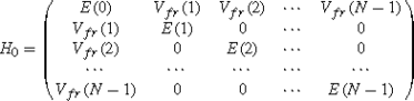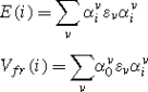
  (17)

  The creation operators of the new basis are given by the set $\{a_{0}^{\dag},a_{i}^{\dag} \}$, (0<i≤N−1). The $a_{i}^{\dag}$ can be expressed in terms of the s-states; $a_{i}^{\dag}=\sum_{\nu=1}^{N}\alpha_{i}^{\nu}c_{\nu}^{\dag}$. The state $a_{0}^{\dag}$ uniquely determines the other states $a_{i}^{\dag}$. The state $a_{0}^{\dag}$ is coupled through the matrix elements V _fr (i) to the states $a_{i}^{\dag}$, which makes the state $a_{0}^{\dag}$ an artificial Friedel resonance. The matrix elements E(i) and V _fr (i) are given as

  

• In the final step (5), the state $a_{0}^{\dag}$ is rotated in the N-dimensional Hilbert space. In each cycle, the state $a_{0}^{\dag}$ is rotated in the $( a_{0}^{\dag},a_{i_{0}}^{\dag} )$ plane by an angle $\theta_{i_{0}}$ for 1≤i ₀≤N−1. Each rotation by $\theta_{i_{0}}$ yields a new $\overline{a_{0}}^{\dag}$

  $$\overline{a_{0}}^{\dag}=a_{0}^{\dag}\cos \theta_{i_{0}}+a_{i_{0}}^{\dag}\sin \theta_{i_{0}}$$

  The rotation leaves the whole basis $\{ a_{0}^{\dag},a_{i}^{\dag } \}$ orthonormal. Step (4), the diagonalization of the (N−1)-sub Hamiltonian, is now much quicker because the (N−1)-sub-Hamiltonian is already diagonal with the exception of the i ₀-row and the i ₀-column. For each rotation plane $(a_{0}^{\dag},a_{i_{0}}^{\dag} )$, the optimal $a_{0}^{\dag}$ with the lowest energy expectation value is determined. This cycle is repeated until one reaches the absolute minimum of the energy expectation value. In the example of the Friedel resonance Hamiltonian, this energy agrees numerically with an accuracy of 10⁻¹⁵ with the exact ground-state energy of the Friedel Hamiltonian [8]. For the FA impurity, the procedure is stopped when the expectation value changes by less than 10⁻¹⁰ during a full cycle.

Appendix C: Changing the Wilson Basis

In NRG, one usually constructs the Wilson states with Λ=2. This means that one uses energy cells whose width reduced by a factor of two. NRG is in principle exact for $\varLambda\thickapprox1$ (together with the requirement that one can diagonalize matrices of gigantic sizes). In the FAIR method, we also begin the calculation with Λ=2. When the fair state $a_{0}^{\dag}$ is obtained for Λ=2 in the basis $\{ c_{\nu }^{\dag} \}$, then it is also approximately known in the original basis $\{ \varphi_{k}^{\dag} \}$ (with 10²³ states)

$$a_{0}^{\dag}={\sum_{\nu=1}^{N}} \alpha_{0}^{\nu}c_{\nu}^{\dag}={\sum_{\nu=1}^{N}}\alpha_{0}^{\nu}{\sum_{\mathfrak{C}_{\nu}}} \varphi_{k}^{\dag}/\sqrt{Z_{\nu}}$$

Now one can choose a smaller Λ, for example $\varLambda=\sqrt{2}$ and interpolate with good accuracy the fair state for the smaller value of Λ [11]. The optimization of the resulting fair state requires now a relatively short additional numerical iteration. For the calculation of the Friedel oscillation, a value of $\varLambda=\sqrt[4]{2}=1.19$ was used.

Appendix D: Geometrical Derivation of the Friedel Ground State

If the conduction electrons are described by a basis of N states then together with the d-state this yields an (N+1)-dimensional Hilbert space ℌ _N+1. The Friedel Hamiltonian is a single particle Hamiltonian and possesses in our case (N+1) orthonormal eigenstates $b_{j}^{\dag}$, which are compositions of the N states $c_{\nu}^{\dag}$ and the one d-state d ^†. The n-electron ground state is then the product of the n creation operator $b_{j}^{\dag}$ with the lowest energy (applied to the vacuum state Φ ₀). These n states define the n-dimensional occupied sub-Hilbert space ℌ _n . The remaining (N+1−n) eigenstates form the complementary unoccupied sub-Hilbert space ℌ _N+1−n . In the following, we treat the creation operators as unit vectors within the Hilbert space.

Now the vector d of the d-state lies partially in the occupied and the unoccupied sub-Hilbert space. It has a projection $\mathbf{d}_{1}^{\prime }$ in the occupied sub-Hilbert space ℌ _n and a projection $\mathbf{d}_{2}^{\prime}$ in the unoccupied sub-Hilbert space ℌ _N+1−n (so that $\mathbf{d}=\mathbf{d}_{1}^{\prime}+\mathbf{d}_{2}^{\prime }$). The lengths of the vectors $\mathbf{d}_{1}^{\prime}$ and $\mathbf{d}_{2}^{\prime}$ are less than one. So, we normalize them to d ₁ and d ₂ with |d _i |=1. These two vectors are orthogonal (they lie in different sub-Hilbert spaces) and form therefore a two-dimensional space. The vector d lies within this plane because

$$\mathbf{d=d}_{1}^{\prime}+\mathbf{d}_{2}^{\prime}=\alpha\mathbf{d}_{1}+\beta\mathbf{d}_{2}$$

The vector perpendicular to d in this plane is the fair state $a_{0}^{\dag}$ with the composition

$$\mathbf{a}_{0}=\beta\mathbf{d}_{1}-\alpha \mathbf{d}_{2}$$

Then the vector d ₁ has the form

$$\mathbf{d}_{1}=\beta\mathbf{a}_{0}+\alpha \mathbf{d}$$

The vector d ₁ can be used as a basis vector of the (N+1) Hilbert space ℌ _N+1. It lies completely within the occupied sub-Hilbert space. Now, we divide the occupied sub-Hilbert space ℌ _n into the one-dimensional space d ₁ and an (n−1)-dimensional subspace $\mathfrak{S}_{n-1}$ which is orthogonal to d ₁. This subspace $\mathfrak{S}_{n-1}$ is also orthogonal to the d-state vector d and is therefore built only of c _ν vectors. It can be decomposed into (n−1) orthonormal basis vectors $\bar{\mathbf{a}}_{i}$.

Returning to the physics, the ground state can be expressed as

$$\varPsi_{F}= \bigl( \beta a_{0}^{\dag}+\alpha d^{\dagger} \bigr) {\prod _{i=1}^{n-1}} \bar{a}_{i}^{\dag}\varPhi_{0}$$

Similarly, the sub-Hilbert space ℌ _N+1−n can be divided into d ₂ and a subspace $\mathfrak{S}_{N-n}$ orthogonal to d ₂ which is therefore also orthogonal to d. $\mathfrak{S}_{N-n}$ can be expressed in terms of (N−n) orthonormal basis vectors $\bar{\mathbf{a}}_{i}$ (which consists only of vectors c _ν ).

The creation operators $\bar{a}_{i}$ are not yet uniquely determined. That is done by diagonalizing the Hamiltonian H ₀ in $\mathfrak{S}_{n-1}$ and $\mathfrak{S}_{N-n}$. This yields the new basis $\{ a_{i}^{\dag },1\leq i<N-1 \}$. It is straight forward to show that the matrix elements $\langle a_{i}^{\dag} \vert H_{0}\vert a_{i^{\prime}}^{\dag} \rangle$ for $a_{i}^{\dag}\in\mathfrak{S}_{n-1}$ and $a_{i^{\prime}}^{\dag}\in\mathfrak{S}_{N-n}$ vanish as well. (We know the matrix elements of H _F between any state in $\mathfrak{S}_{N-n}$ and any state in $\mathfrak{S}_{n-1}$ vanishes because the two sub-Hilbert spaces are built from a different subset of eigenstates of H _F . Therefore, $\langle a_{i}^{\dag} \vert H_{F}\vert a_{i^{\prime}}^{\dag } \rangle =0$ if $a_{i}^{\dag}\in\mathfrak{S}_{n-1}$ and $a_{i^{\prime}}^{\dag}\in\mathfrak{S}_{N-n}$. Since $\mathfrak{S}_{n-1}$ and $\mathfrak{S}_{N-n}$ are orthogonal to d ^†, the d component of the Hamiltonian H _F vanishes anyhow and the remaining part $\langle a_{i}^{\dag }\vert H_{0}\vert a_{i^{\prime}}^{\dag} \rangle =0$ vanishes for all pairs of i and i′.)

References

Friedel, J.: Adv. Phys. 3, 446 (1954)
Friedel, J.: Philos. Mag. 43, 153 (1952)
Friedel, J.: Can. J. Phys. 34, 1190 (1956)
Friedel, J.: J. Phys. Radium 19, 573 (1958)
Friedel, J.: Suppl. Nuovo Cim. 7, 287 (1958)
Anderson, P.W.: Phys. Rev. 124, 41 (1961)
Hewson, A.C.: The Kondo Problem to Heavy Fermions. Cambridge University Press, Cambridge (1993)
Bergmann, G.: Z. Phys. B 102, 381 (1997)
Bergmann, G.: Eur. Phys. J. B 2, 233 (1998)
Wilson, K.G.: Rev. Mod. Phys. 47, 773 (1975)
Bergmann, G.: Phys. Rev. B 78, 195124 (2008)
Tao, Y., Bergmann, G.: Eur. Phys. J. B 85, 42 (2012)
Blandin, A., Friedel, J.: J. Phys. Radium 20, 160 (1959)
Kondo, J.: Prog. Theor. Phys. 32, 37 (1964)
Schrieffer, J.R., Wolff, P.A.: Phys. Rev. 149, 491 (1967)
Krishna-Murthy, H.R., Wilkins, J.W., Wilson, K.G.: Phys. Rev. B 21, 1003 (1980)
Bergmann, G.: Phys. Rev. B 74, 144420 (2006)
Kwon, S.K., Min, B.I.: Phys. Rev. Lett. 84, 3970 (2000)
Bergmann, G.: Eur. Phys. J. B 75, 497 (2010)
Oguchi, A.: Prog. Theor. Phys. 43, 257 (1970)
Brenig, W., Schoenhammer, K.: Z. Phys. 267, 201 (1974)
Logan, D.E., Eastwood, M.P., Tusch, M.A.: J. Phys., Condens. Matter 10, 2673 (1998)
Yosida, K.: Phys. Rev. 147, 223 (1966)
Varma, C.M., Yafet, Y.: Phys. Rev. B 13, 2950 (1976)
Schoenhammer, K.: Phys. Rev. B 13, 4336 (1976)
Daybell, M.D., Steyert, W.A.: Rev. Mod. Phys. 40, 380 (1968)
Heeger, A.J.: In: Seitz, F., Turnbull, D., Ehrenreich, H. (eds.) Solid State Physics, vol. 23, p. 284. Academic Press, New York (1969)
Maple, M.B.: In: Rado, G.T., Suhl, H. (eds.) Magnetism, vol. V, p. 289. Academic Press, New York (1973)
Anderson, P.W.: Rev. Mod. Phys. 50, 191 (1978)
Gruener, G., Zawadowski, A.: Prog. Low Temp. Phys. 7B, 591 (1978)
Coleman, P.: J. Magn. Magn. Mater. 47, 323 (1985)
Anderson, P.W.: J. Phys. C 3, 2436 (1970)
Frota, H.O., Oliveira, L.N.: Phys. Rev. B 33, 7871 (1986)
Krishna-Murthy, H.R., Wilkins, J.W., Wilson, K.G.: Phys. Rev. B 21, 1044 (1980)
Nozieres, P.: J. Low Temp. Phys. 17, 31 (1974)
Nozieres, P.: Ann. Phys. (Paris) 10, 19 (1985)
Newns, D.M., Read, N.: Adv. Phys. 36, 799 (1987)
Gunnarsson, O., Schoenhammer, K.: Phys. Rev. B 28, 4315 (1983)
Bickers, N.E.: Rev. Mod. Phys. 59, 845 (1987)
Wiegmann, P.B.: In: Lifshitz, I.M. (ed.) Quantum Theory of Solids, p. 238. MIR Publishers, Moscow (1982)
Andrei, N., Furuya, K., Lowenstein, J.H.: Rev. Mod. Phys. 55, 331 (1983)
Schlottmann, P.: Phys. Rep. 181, 1 (1989)
Nilsson, J., Neto, A.H.C., Guinea, F., Peres, N.M.R.: Phys. Rev. Lett. 97, 266801 (2006)
Gunnarsson, O., Schoenhammer, K.: Phys. Rev. B 31, 4815 (1985)
Bergmann, G., Zhang, L.: Phys. Rev. B 76, 064401 (2007)
Bergmann, G.: Phys. Rev. B 77, 104401 (2008)
Boyce, J.B., Slichter, C.P.: Phys. Rev. Lett. 32, 61 (1974)
Affleck, I., Simon, P.: Phys. Rev. Lett. 86, 2854 (2001)
Simon, I.P., Affleck, I.: Phys. Rev. Lett. 89, 206602 (2002)
Pereira, R.G., Laflorencie, N., Affleck, I., Halperin, B.I.: arXiv:cond-mat/0612635 (2007)
Simonin, J.: arXiv:0708.3604 (2007)
Bergmann, G., Tao, Y.: Eur. Phys. J. B 73, 95 (2010)
Bergmann, G., Thompson, R.S.: Eur. Phys. J. B 84, 273 (2011)
Weichselbaum, A., Münder, W., Delft, J.V.: Phys. Rev. B 84, 075137 (2011)
Affleck, I., Borda, L., Saleur, H.: Phys. Rev. B 77, 180404(R) (2008)
Author information
Authors and Affiliations
Corresponding author