
Abstract
Two zonal high-density hydrographic sections along 41° N and 37.5° N east of Japan were occupied in April 2013 and June 2016 to examine the formation of Central Mode Water (CMW) and Transition Region Mode Water (TRMW) in relation to fronts and eddies. In the 41° N section traversing the meandering subarctic front, the denser variety of CMW (D-CMW) and TRMW was formed continuously on both sides of the front, except for the part of the section located south of the Kuroshio bifurcation front where the lighter variety of CMW (L-CMW) and D-CMW was formed instead. L-CMW and D-CMW were also formed in the eastern part of the 37.5° N section between the Kuroshio Extension front and the Kuroshio bifurcation front, but were hardly formed in the western part of the section west of the bifurcation point of the two fronts. D-CMW and TRMW pycnostads in the western part of the 41° N section observed in April 2013 tended to exhibit more than one core (vertical minimum of potential vorticity), which might be formed by destruction of deep winter mixed layers. Such multiple-core structure was also observed in L-CMW and D-CMW pycnostads in the eastern part of both the sections south of the Kuroshio bifurcation front in June 2016, being particularly abundant in three anticyclonic eddies. It was likely to be formed by the exchange of low-potential vorticity water among the eddies and the ambient region in association with eddy-to-eddy interaction, suggesting a new mechanism of mode water subduction.
1 Introduction
Central Mode Water (CMW; Nakamura 1996; Suga et al. 1997) is a low-potential vorticity (Q) water found in the lower permanent pycnocline of the North Pacific subtropical gyre. It is formed as deep winter mixed layers north of the Kuroshio Extension, subducted in the central northern part of the subtropical gyre, and transported anticyclonically toward the western boundary (Suga et al. 2004; Oka et al. 2011a). The formation, subduction, and circulation of CMW and their temporal variability are believed to be important for various physical and biogeochemical processes over the North Pacific (Oka and Qiu 2012; Oka et al. 2014).
Since CMW was identified, efforts have been made to clarify how the water is formed in the Kuroshio–Oyashio Extension region characterized by several thermohaline fronts (Yasuda 2003; Nakano et al. 2018): the Kuroshio Extension front (KEF), the Kuroshio bifurcation front (KBF), the subarctic front (SAF; Roden 1970, 1972; Yuan and Talley 1996), and the polar front (PF; Favorite et al. 1976; Belkin et al. 2002) from the south to the north. Oka and Suga (2005) analyzed the repeat hydrographic section along 165° E in 1991–2003 to demonstrate that the lighter variety of CMW (L-CMW) with potential temperature (θ) of 11°–14 °C, salinity (S) of 34.3–34.6, and potential density (σθ) of 25.8–26.2 kg m−3 is formed between the KEF and the KBF, while its denser variety (D-CMW) with θ = 8°–10 °C, S = 34.0–34.2, and σθ = 26.3–26.4 kg m−3 is formed between the KBF and the SAF, as suggested by an earlier observation (Mecking and Warner 2001) and an analysis of ocean general circulation model output (Tsujino and Yasuda 2004). Furthermore, Saito et al. (2007) examined several hydrographic sections at 158°–162° E carried out in July 2002 to reveal the existence of a colder, fresher, and denser low-Q water with θ = 5°–7 °C, S = 33.5–33.9, and σθ = 26.5–26.6 kg m−3 in the subtropical-subarctic transition region, and named it Transition Region Mode Water (TRMW). Unlike CMW, TRMW is not observed in the permanent pycnocline in the subtropical gyre (Suga et al. 2004), possibly because it is rapidly modified to D-CMW after formation due to double-diffusion salt-finger convection (Saito et al. 2011).
It then became possible to examine the formation and subduction of CMW/TRMW using temperature (T) and S data from Argo profiling floats (Roemmich et al. 2001; Riser et al. 2016). A composite analysis of Argo data in 2003–2008 (Oka et al. 2011a) demonstrated that L-CMW (D-CMW and TRMW) was formed in a zonally-elongated band of deep winter mixed layers at 33°–39° N (39°–43° N) extending from the east coast of Japan (~ 142° E) to 160° W, and was subducted to the permanent pycnocline from the eastern part (east of 170° E) of each band. In contrast, an analysis of contemporary hydrographic sections occupied by several research vessels over the CMW/TRMW formation region in spring 2003 (Oka et al. 2014) exhibited a quite different distribution of these waters. Specifically, TRMW and D-CMW were formed extensively south of the SAF between 155° E and 165° W, but formed only in two anticyclonic mesoscale eddies west of 155° E. L-CMW was formed only in the region south of the KBF and east of 165° E. Such a difference in the CMW/TRMW distribution between the multi-year Argo data and the synoptic shipboard survey suggests that the formation of these waters in the western part of their formation regions occurs only in anticyclonic eddies, which is supported by a positive correlation between the winter mixed layer depth and sea surface height (SSH) observed in this latitude band (Kouketsu et al. 2012).
To further clarify the relation of the CMW/TRMW formation to the fronts and eddies, we need more hydrographic sections with sufficient spatial resolution, particularly zonal ones, as many existing sections ran meridionally to cross the zonal fronts. We, therefore, carried out two cruises in April 2013 and June 2016 to occupy two zonal high-resolution sections traversing the western part of the L-CMW and D-CMW/TRMW formation regions presented by Oka et al. (2011a). In this study, we analyze data from these cruises to examine the detailed structure of CMW/TRMW just after formation in relation to the fronts and eddies.
2 Observation and data
The KH-13-3 cruise of R/V Hakuho-maru was implemented from April 2 through May 1, 2013. Its main objective was to conduct a zonal section along 41° N between the east coast of Japan and 170° E crossing the western part of the assumed D-CMW/TRWM formation region. However, due to bad sea conditions throughout the cruise, the zonal section was occupied only from 41° N, 161° E to 42° N, 151° E (called the 41° N-west section hereafter; Fig. 1a, b) on April 13–17. Along the section, T, S, and dissolved oxygen were measured down to 2000 dbar by a conductivity-temperature-depth-oxygen profiler (CTDO2; Sea-Bird Scientific SBE 9plus equipped with SBE 43) at intervals of 1° in longitude, except at 151° E and additionally at 155°30′ E. At the CTDO2 stations, discrete water samples were collected for measurements of S, dissolved oxygen and its isotope ratio, nutrients, dissolved inorganic carbon, total alkalinity, chlorophyll-a, and volatile organic compounds. Phytoplankton productivity was also measured down to 200 dbar by a fast repetition rate fluorometry, and turbulence was recorded down to about 500 dbar by a microstructure profiler. Between the CTDO2 stations, T and S were measured down to 1100 dbar by an expendable conductivity-temperature-depth profiler (XCTD; Tsurumi Seiki XCTD-1) at intervals of 10′ in longitude. In addition, meteorological observations were made along the section (Kawai et al. 2019).

Locations of CTDO2 (open circles) and XCTD (closed circles) stations of the KH-13-3 (a, b) and KH-16-3 (c, d) cruises. The background contours with color represent SSH (a, c; contour interval = 10 cm) and SST (b, d; contour interval = 1 °C) on April 15, 2013 (a, b) and June 14, 2016 (c, d). The dashed lines indicate the zonal sections of the KH-16-3 (a, b) and KH-13-3 (c, d) cruises. A, B, and C in c denote Eddies A–C
The KH-16-3 cruise of R/V Hakuho-maru was performed from May 31 through June 29, 2016. Its main target was to extend the zonal section of the KH-13-3 cruise eastward and to conduct a zonal section along 37.5° N between the east coast of Japan and 170° E crossing the western part of the assumed L-CMW formation region. Thanks to fine weather, we occupied a quasi-zonal section from 41° N, 161° E to 40.1° N, 170° E (called the 41° N-east section hereafter) on June 6–10 and another zonal section along 37.5° N from 170° E to 143° E (the 37.5° N section) on June 14–27 (Fig. 1c, d). Along both sections, CTDO2 observations were made down to 2000 dbar at intervals of 1° in longitude and additionally down to the bottom (~ 5300 dbar) at 168°40′ E and 169°10′ E. At the CTDO2 stations, discrete water samples were collected for measurements of S, dissolved oxygen and its isotope ratio, nutrients, dissolved inorganic carbon, total alkalinity, chlorophyll-a, methane, nitrate isotope ratio, dissolved radioactive cesium (Aoyama et al. 2018), and suspended particles. Turbulence was also measured down to about 1000 dbar by a microstructure profiler (Goto et al. 2018). Between the CTDO2 stations, XCTD observations were made at intervals of 10′ in longitude. In addition, meteorological variables and bacterial concentration in marine air (Hu et al. 2017) were measured along the sections.
Along the three sections, current velocity was measured by a shipboard acoustic Doppler current profiler (ADCP; Teledyne RDI Ocean Surveyor 38 kHz) at depth intervals of 16 m and was calibrated as explained in Joyce (1989). The ADCP velocity data with good quality were obtained down to 640 m at the 41° N-west and 37.5° N sections and down to 480 m at the 41° N-east section when the zonal ship speed exceeded 5 m s−1. We, therefore, averaged zonal and meridional ADCP velocities with the zonal ship speed > 5 m s−1 in each bin of 10′ in longitude between the CTDO2/XCTD stations after excluding anomalous values beyond 2.5 standard deviations from the mean.
From T, S, and dissolved oxygen data obtained at the CTDO2/XCTD stations of the three sections, we calculated θ, σθ, in situ water density (ρ), and apparent oxygen utilization (AOU). Geostrophic velocity normal to the sections was calculated using a reference level of 1000 dbar after ρ was horizontally smoothed along each section using a three-point Hanning filter with weights of 0.25, 0.5, and 0.25. The vertical shear of geostrophic velocity matched well with that of ADCP velocity normal to the sections at depths greater than 150 m (not shown). We, therefore, calculated barotropic velocity as the difference between the ADCP and geostrophic velocities averaged at depths of 160–400 m, and added it to the geostrophic velocity at all depths to obtain absolute geostrophic velocity. Finally, Q was calculated on the basis of the definition
where f is the Coriolis parameter, V the absolute geostrophic velocity normal to the sections (positive north-northeastward or northward), X the along-section coordinate (positive east-southeastward or eastward), z the vertical coordinate (positive upward), g the gravity acceleration, and p is pressure. The vertical gradient of σθ at pressure p was computed from σθ between p − 25 dbar and p + 25 dbar using the linear least squares method. In this study, we defined a pycnostad in each CTD/XCTD profile as a layer with Q < 1.5 × 10⁻¹⁰ m−1 s−1 and thicker than 50 dbar, following the previous studies on CMW/TRMW (Oka and Suga 2005; Saito et al. 2011).
We used SSH data produced and distributed by the Copernicus Marine and Environment Monitoring Service (Ducet et al. 2000, https://www.marine.copernicus.eu) and sea surface temperature (SST) data provided by the Japan Meteorological Agency as the Merged Satellite and In-situ Data Global Daily Sea Surface Temperature (Sakurai et al. 2005). Both data are provided daily on a 0.25° × 0.25° grid. We also used T, S, and dissolved oxygen data obtained by an Argo profiling float with World Meteorological Organization identifier (WMO ID) 5904036 in 2016, and T and S data from Argo floats near the 41° N-west and 41° N-east sections in 2013 and 2016. These data were downloaded from the ftp site of the Argo Global Data Assembly Center (ftp://usgodae.org/pub/outgoing/argo, ftp://ftp.ifremer.fr/ifremer/argo, https://doi.org/10.17882/42182) and edited as outlined in Oka et al. (2007).
3 Current and hydrographic structure around the zonal sections
The 41° N-west and 41° N-east sections were located near the subtropical–subarctic boundary, which was well represented by sea surface S of 33.8 (Fig. 2b). Subtropical water characterized by the subsurface S minimum existed at the stations with surface S > 33.8, while subarctic water characterized by the S minimum at the surface was found at stations with surface S < 33.8. At 151°45′ E, 161°55′ E. 163°15′ E, 164°35′ E, and 165°50′ E, the two waters were separated by a density-compensating sharp S and θ front near the sea surface (Fig. 2a–c). This is the SAF, characterized by the outcrop of S = 33.0–33.8 isohalines constituting the subarctic permanent halocline (Roden 1970, 1972; Yuan and Talley 1996) and accompanied by eastward flow (Niiler et al. 2003; Nakano et al. 2018). The western part of the 41° N-east section traversed the meandering SAF, which was reflected in meandering SST contours (Fig. 1d) and alternating southeastward and northeastward flow between 161° E and 166° E (Fig. 3a, b).

Distributions of a θ, b S, c σθ, and d Q with respect to pressure and e Q with respect to σθ in the 41° N-west (left) and 41° N-east (right) sections. Contour interval is a 1 °C, b 0.1, and c 0.1 kg m−3. Contours are drawn at 0.5, 1, 1.5, 2, 3, and 5 × 10⁻¹⁰ m−1 s−1 in d and e. Dots in b represent vertical S minimum at each station. Long (short) ticks on the top of each panel indicate the locations of CTDO2 (XCTD) stations. Arrows (horizontal bars) on the top of each panel in a represent the locations of fronts (Eddies A–C)

Distributions of a eastward and b northward ADCP velocity and c absolute geostrophic velocity normal to the section (positive north-northeastward) in the 41° N-west (left) and 41° N-east (right) sections. Contour interval is 10 cm s−1. N, S, E, and W in a and b denote northward, southward, eastward, and westward flow, respectively. Long (short) ticks on the top of each panel indicate the locations of CTDO2 (XCTD) stations. Arrows (horizontal bars) on the top of each panel in a represent the locations of fronts (Eddies A–C)
The most intense SAF at 151°45′ E was also the PF, as it was associated with the 4 °C isotherm standing almost vertically down to 250-dbar depth and the subsurface temperature minimum occurring to its west (Fig. 2a, b). Absolute geostrophic velocity exhibited a north-northeastward flow faster than 10 cm s−1 between 151°20′ E and 152°10′ E with the peak of 18 cm s−1 at 151°55′ E immediately east of the front (Fig. 3c). This is considered to be the quasi-stationary jet along the PF, the so-called Isoguchi jet, that transports warm and saline subtropical water northward (Isoguchi et al. 2006; Wagawa et al. 2014; Mitsudera et al. 2018; Miyama et al. 2018). The eastern part of the 41° N-west section between 156° E and 160° E crossed the northern part of a weak cyclonic circulation (Fig. 1a), and was associated with a southwestward flow between 156° E and 158° E and a northwestward flow between 158° E and 161° E (Fig. 3a, b) as well as the shallower permanent pycnocline centered at 158° E (Fig. 2c). The southwestward flow between 156° E and 158° E likely advected the colder and fresher subarctic water (Fig. 2a, b) from the north, as also indicated by the SST map (Fig. 1b).
The eastern part of the 41° N-east section traversed the northern part of an anticyclonic eddy centered at 40° N, 168° E (called Eddy A hereafter; Fig. 1c). The maximum northward (southward) surface geostrophic flow in the western (eastern) part of Eddy A was 23 (60) cm s−1 at 168°05′ E (169°15′ E) (Fig. 3c). To the west of Eddy A, there existed another northward flow as fast as 35 cm s−1 centered at 166°30′ E, where θ at 300-dbar depth was 7.2 °C (Fig. 2a). This flow was considered to be the KBF, which is associated with θ = 6°–8 °C at 300-dbar depth (Mizuno and White 1983). In fact, the SSH contour of 60 cm that traversed the 41° N-east section at 166°30′ E traced back to 37° N, 158° E, where it bifurcated from the KEF (Fig. 1c). To the downstream, the same SSH contour surrounded Eddy A and merged into the eddy in its eastern part, which was observed as the single southward flow centered at 169°15′ E in the 41° N-east section (Fig. 3c).
The 37.5° N section was located north of the meandering KEF, except at 143°–146° E and 147°–149.5° E where it traversed a strong anticyclonic eddy just detached from the Kuroshio Extension and the northern edge of the Kuroshio Extension, respectively (Figs. 1c, 5). Subtropical water with the subsurface S minimum at depths of 200–700 dbar was seen throughout the section (Fig. 4a). An inconspicuous but important feature is the northward current of 25 cm s−1 at 158°15′ E (Fig. 5c), which is considered to be the above-mentioned KBF immediately after its detachment from the KEF (Fig. 1c). The main thermocline and pycnocline and the S minimum layer were considerably deeper on the eastern side of the KBF than the western side (Fig. 4a–c), which was also reflected in the larger SSH along the 37.5° N section on the eastern side of the KBF (Fig. 1c). East of the KBF, the 37.5° N section crossed two anticyclonic eddies (Fig. 1c): an eddy at 164° E (called Eddy B hereafter) and the northern part of another eddy at 169° E (Eddy C). The maximum northward (southward) geostrophic flow in the western (eastern) part was 41 (26) cm s−1 at 162°55′ E (164°35′ E) for Eddy B and 25 (35) cm s−1 at 168°45′ E (169°55′ E) for Eddy C (Fig. 5c). The horizontal range between the two velocity maxima will be regarded as each eddy in the following sections.

Distributions in the 37.5° N section, otherwise following Fig. 2

Distributions of a eastward and b northward ADCP velocity and c absolute geostrophic velocity normal to the section (positive northward) in the 37.5° N section, otherwise following Fig. 3
4 Distribution and characteristics of pycnostads in the zonal sections
In the 41° N-west section in early spring, pycnostads with Q < 1.5 × 10⁻¹⁰ m−1 s−1 and thicker than 50 dbar spread continuously from 151°50′ E just east of the SAF to 161° E between the sea surface and 200–380 dbar, and were separated from the deep low-Q layer by a thin, relatively high-Q layer (Fig. 2d). The σθ of pycnostads slightly exceeded 26.6 kg m−3 at 154°–157° E, and decreased to both the west and the east (Fig. 2e). In the 41° N-east section in early June, pycnostads also spread almost continuously below the high-Q seasonal pycnocline, regardless of location relative to the SAF, and were thick south of the KBF between 166°30′ and 169°15′ E (Fig. 2b, d). The σθ of pycnostads was ~ 26.4 kg m−3 in the western part of the 41° N-east section, showing apparent discontinuity with the 41° N-west section at 161° E (Fig. 2e), which will be discussed in Sect. 5. In Eddy A located at 168°05′–169°15′ E, Q minima appeared in two σθ ranges of 26.1–26.2 and 26.3–26.4 kg m−3, overlapping each other.
The pycnostad distribution at the 37.5° N section was considerably different between the western and eastern sides of the KBF at 158°15′ E. The eastern part of the section encountered several mesoscale low-Q patches in the σθ range of 26.0–26.4 kg m−3 below the high-Q seasonal pycnocline (Fig. 4d, e). In particular, Eddy B at 162°55′–164°35′ E and Eddy C at 168°45′–169°55′ E contained thick low-Q patches, within which three vertical Q minima overlapped each other. On the western side of the KBF, in contrast, small-scale low-Q patches were observed sparsely below the seasonal pycnocline. Most of them were thinner than 50 dbar and, therefore, not categorized as pycnostads.
In each pycnostad, the core, defined as a Q minimum, is considered to be the least modified portion since the pycnostad was formed, thus best preserving the water properties at the time of formation while the pycnostad is modified through mixing with surrounding water (Talley and Raymer 1982; Suga et al. 1989). Observations of Subtropical Mode Water (Masuzawa 1969) south of the Kuroshio Extension have demonstrated that pycnostads sometimes have two or more cores (Taneda et al. 2000; Oka et al. 2011b; Gao et al. 2016; Liu et al. 2017, 2019), as observed in those in Eddies A, B, and C (Figs. 2d, e, 4d, e). The multiple-core structure in these eddies is more clearly delineated in CTDO2 profiles near the eddy centers,Footnote 1 in each of which three distinct cores existed and were accompanied by AOU minima (Fig. 6).
To examine the occurrence of multiple cores in pycnostads throughout the three sections, we followed the previous studies (Oka et al. 2011b; Liu et al. 2017, 2019) to define a core in a pycnostad as the Q minimum being less than 1.5 × 10⁻¹⁰ m−1 s−1 and having a magnitude of 0.25 × 10⁻¹⁰ m−1 s−1 between depths of 50 dbar and σθ = 26.7 kg m−3, excluding shallow surface mixed layers and intermediate waters that are not outcropped in the open North Pacific (Talley 1988; Suga et al. 2004). If more than one core was detected in a CTD/XCTD profile, they were called the 1st, 2nd, … core in order of increasing Q.
The detected occurrence of multiple cores was different among parts of the sections (Fig. 7 and Table 1). In the 41° N-west section, multiple cores were seen at 38% (= 20/53) of the CTD/XCTD stations with pycnostads. In the 41° N-east section, in contrast, multiple cores hardly occurred, except south of the KBF where they were observed at 63% (= 10/16) of stations with pycnostads and particularly in Eddy A with a higher ratio of 75% (= 6/8). In the eastern part of the 37.5° N section east of the KBF at 158°15′ E, multiple cores almost always occurred in Eddies B and C, but much less frequently (16% = 6/37) in the other parts. The western part of the 37.5° N section west of the KBF exhibited few pycnostads and no multiple cores. After all, multiple cores were abundant in the three eddies south of the KBF. To the north of the KBF, they were observed at the 41° N-west section, but were hardly seen at the 41° N-east section (without Eddy A). The formation mechanism of these multiple cores will be discussed in Sect. 5.
In which year was each of these cores formed in late winter? Past studies have utilized AOU at the core to estimate the age of pycnostads (e.g., Suga et al. 1989; Oka and Suga 2005). Since the zonal resolution (1°) of AOU distributions in the three sections based on CTDO2 measurements (not shown) does not match with that (10′) of the Q distributions based on high-resolution CTDO2/XCTD measurements (Figs. 2d, e, 4d, e), Q and AOU at the cores of pycnostads were compared at the CTDO2 stations (Fig. 8). The cores with the lowest Q < 0.5 × 10⁻¹⁰ m−1 s−1 were mostly associated with low AOU < 0.5 ml l−1. AOU tended to increase as Q increased, which implies that low-Q and low-AOU core waters formed in the late winter of the same year (2013 for the 41° N-west section and 2016 for the 41° N-east and 37.5° N sections) have mixed with high-Q and high-AOU surrounding waters formed in the late winter of the previous years. At Q > 0.8 × 10⁻¹⁰ m−1 s−1, there also existed cores with AOU much higher than 1.0 ml l−1. Such high AOU values indicate that these cores were aged 1 or more years, assuming the oxygen utilization rate of 0.5 ml l−1 year−1 (Jenkins 1980; Suga et al. 1989). The linear least square fitting for plots with Q < 0.8 × 10⁻¹⁰ m−1 s−1 (dashed line in Fig. 8) exhibited a gradual AOU increase with increasing Q. Therefore, it seems reasonable to regard the cores close to this relation (specifically, those with AOU < 0.8 ml l−1) as formed in the late winter of the same year (called “new” hereafter) and the cores with AOU > 0.8 ml l−1 as formed in the previous years (“old”). Plotting core AOU values in the Q distribution (Fig. 9) indicates that the cores of the major pycnostads in the three sections were mostly new. The only old cores found in the major pycnostads were located at σθ = ~ 26.6 kg m−3, 154° E in the 41° N-west section and at σθ = ~ 26.4 kg m−3, 167° and 168° E in Eddy A in the 41° N-east section.

Plots of AOU against Q at the cores of pycnostads in the 41° N-west (closed triangles), 41° N-east (dots), and 37.5° N (open squares) sections. Dashed line represents the linear least squares fitting to the points with Q < 0.8 × 10⁻¹⁰ m−1 s−1

Plots of σθ (dots) at the cores of pycnostads against longitude in the a 41° N-west, b 41° N-east, and c 37.5° N sections. Color dots represent AOU (ml l−1) at the cores at the CTDO2 stations. Black dots denote the cores at the XCTD stations without dissolved oxygen measurements. In the background, Q contours of 0.5, 1, 1.5, and 2 × 10⁻¹⁰ m−1 s−1 are drawn, and the areas with Q < 1.5 × 10⁻¹⁰ m−1 s−1 are lightly hatched. Long (short) ticks, arrows, and horizontal bars on the top of each panel indicate the locations of CTDO2 (XCTD) stations, fronts, and Eddies A–C, respectively
Finally, what types of mode water were these cores classified into? Previous studies on CMW/TRMW (Saito et al. 2007, 2011; Oka et al. 2011a) have demonstrated that the properties of these waters exhibit a near-linear relation on a θ–S diagram, with the approximate boundary between TRMW and D-CMW (D-CMW and L-CMW) at θ = 7.5 °C, S = 33.90 (θ = 10.5 °C, S = 34.25). If we apply these criteria to the core θ/S distributions in the three sections (Fig. 10), the cores at the 41° N-west and 41° N-east sections were mostly TRMW and partly D-CMW, except south of the KBF where D-CMW and L-CMW cores existed, overlapping each other in Eddy A. The eastern part of the 37.5° N section east of the KBF was associated with L-CMW and D-CMW cores, which coexisted and overlapped each other in Eddies B and C.

Plots of a θ and b S at the cores of pycnostads against longitude in the 41° N-west (closed triangles), 41° N-east (dots), and 37.5° N (open squares) sections. Long (short) ticks, arrows, and horizontal bars on the top of panel in a indicate the locations of CTDO2 (XCTD) stations, fronts, and Eddies A–C, respectively, in the 41° N-west and 41° N-east sections, while those on the top of panel in b denote their locations in the 37.5° N section
5 Discussion
Multiple cores have been observed in Subtropical Mode Water pycnostads and thought to be formed by interleaving of mode waters with different densities (Oka et al. 2011b) or by formation of a lighter mode water over a preexisting denser mode water (Liu et al. 2017, 2019). In our cruises in 2013 and 2016, they were observed in 38% of TRMW/D-CMW pycnostads in the 41° N-west section in mid-April, but were hardly seen in the 41° N-east section except south of the KBF in early June (Fig. 7 and Table 1). Such a contrast suggests that the 41° N-west section offered favorable conditions for the generation of multiple cores. In the continuous TRMW/D-CMW pycnostads at the 41° N-west section, an old core with AOU > 0.8 ml l−1 was observed only at 154° E (Fig. 9). At this CTDO2 station, a new core with σθ = 26.50 kg m−3 was formed at 120 dbar over the old core with σθ = 26.62 kg m−3 at 220 dbar (Fig. 11a). At the other CTDO2 stations, two new cores overlapped each other in a vertical profile where θ and S changed in a compensating way with small σθ changes, a typical hydrographic feature near the SAF (Fig. 11b, c). There were both cases of a low-θ and low-S core overlying a high-θ and high-S core (Fig. 11b) and those of a high-θ/S core overlying a low-θ/S core (Fig. 11c). Such structures might be formed by destruction of deep winter mixed layers in regions near the SAF where subtropical and subarctic waters are adjacent with each other, possibly due to horizontal advection or baroclinic/symmetric instability. After formation, the multiple-core structure probably disappeared quickly due to the development of seasonal pycnocline and vertical mixing, as inferred from its absence in the 41° N-east section in early June.

Vertical profiles of (upper panel) σθ (thick line), θ (thin line), and S (dashed line) and (lower panel) Q (thick line) and AOU (thin line) obtained by CTDO2 at a 154° E, b 156° E, and c 161° E of the 41° N-west section. Arrows in the lower panel indicate the cores of a pycnostad. Dashed line in the lower panel represents Q = 1.5 × 10⁻¹⁰ m−1 s−1 and AOU = 0.8 ml l−1, as in Fig. 6
If so, how were the abundant multiple cores in Eddies A, B, and C observed in early to mid-June formed? As mentioned in Sect. 4, each CTDO2 profile near the center of these eddies exhibited three cores, out of which only the lower core in Eddy A was old (Fig. 6). Further examination reveals that properties of the upper core in Eddy A (σθ = 26.17 kg m−3, θ = 11.4 °C, S = 34.32) corresponded to those of the middle core in Eddy B (26.18 kg m−3, 11.4 °C, 34.33) and Eddy C (26.19 kg m−3, 11.2 °C, 34.29), and those of the middle core in Eddy A (26.32 kg m−3, 9.9 °C, 34.15) agreed with those of the lower core in Eddy B (26.32 kg m−3, 9.8 °C, 34.15) and Eddy C (26.33 kg m−3, 9.7 °C, 34.13), which implies that each group of cores had the same origin. When we look at SSH distributions for half a year prior to our cruise in June 2016 (Fig. 12), these eddies bunched together in January and February, broke into three in mid-March, merged again in late April, and split again in early June. It is likely that pycnostad waters had been transferred and shared among these eddies and the ambient region during this course of time.

Distributions of SSH (contours with color as in Fig. 1a, c) at intervals of two weeks from January 6 through June 8, 2016. Open (closed) circles denote the locations of CTDO2 (XCTD) stations of the KH-16-3 cruise. Closed squares represent the observation locations of an Argo profiling float with WMO ID 5904036 from seven days before the SSH observation date through six days after it. A, B, and C in d–l denote Eddies A–C
Such an idea is supported by CTDO2 observationsFootnote 2 by an Argo profiling float with WMO ID 5904036, which was trapped in Eddy C until the end of June (closed squares in Fig. 12) and left the eddy in early July. The float observed the densest mixed layer with σθ = 26.07 kg m−3 on April 4, which remained as a low-Q layer with low AOU in the following period (Fig. 13). In addition, a denser low-Q and low-AOU layer with σθ = 26.2–26.3 kg m−3 appeared in the subsurface on March 17 and remained underneath the locally formed low-Q layer. This intrusion occurred when the bunched eddies deformed and then broke into three (Fig. 12e, f), which suggests that low-Q water was entrained into Eddy C from the other eddies and the ambient region in association with the deformation and splitting of the eddies.

Time–pressure sections of a θ, b S, and c Q and time–σθ sections of d Q and e AOU obtained by an Argo profiling float with WMO ID 5904036 from January 4 through July 8, 2016. Contour interval is 1 °C in a, 0.1 in b, and 0.1 ml l−1 for values < 2.0 ml l−1 and 0.5 ml l−1 for values > 2.0 ml l−1 in e. Contours are drawn at 0.5, 1, 1.5, 2, 3, and 5 × 10⁻¹⁰ m−1 s−1 in c and d. Dots in c–e denote the cores of pycnostads detected as explained in Sect. 4
It is thus expected for Eddy C (Fig. 6c) that the upper core at σθ = 26.09 kg m−3 was locally formed, while the middle and lower cores at σθ = 26.19 and 26.33 kg m−3 were formed outside of the eddy and then intruded. The same seems to apply for Eddy B with the upper core at σθ = 26.04 kg m−3 (Fig. 6b). The upper core in Eddy A (Fig. 6a) was the shallowest, and was likely to be locally formed and then transferred to Eddies B and C to constitute their middle core. The remaining question is where the middle core in Eddy A and the lower core in Eddies B and C at σθ = 26.32–26.33 kg m−3 were formed. On the 37.5° N section, pycnostads with a single core with similar properties (σθ = 26.30–26.35 kg m−3, θ = 9.1–9.7 °C, S = 34.03–34.13) spread at 166°40′–167°40′ E between Eddies B and C (Fig. 7). These waters were possibly transferred to the three eddies to constitute their middle/lower core. In summary, the only upper core of each eddy seemed to be locally formed, overlying the middle and lower cores that were remotely formed and then intruded. Our observations suggest a new mechanism of mode water subduction associated with eddy-to-eddy interaction.
Another issue raised in Sect. 4 is the discontinuity in the core σθ of pycnostads between the 41° N-west and 41° N-east sections at 161° E (Figs. 2e, 7a,b). When we plot the core properties on a θ–S diagram, the cores in the 41° N-west section in April 2013 were located on the saltier, colder, and denser side than the 41° N-east and 37.5° N sections in June 2016 (Fig. 14a). This difference should have originated in their formation regions because deep winter mixed layers near the 41° N-west and 41° N-east sections in the respective years observed by Argo profiling floats exhibited similar θ–S distributions to the cores (Fig. 14b). The denser winter mixed layers in 2013 were possibly due to higher S and/or lower θ, but SST around the 41° N-west and 41° N-east sections in the late winter of 2013 tended to be higher than in 2016 (Fig. 15). It is, therefore, expected that the difference in the mixed layer σθ between the two years was due to that in mixed layer S. Such an effect of interannually varying S on the mixed layer σθ might be important, particularly because the 41° N-west section is the place where the deepest winter mixed layers and the densest mode waters are formed in the open North Pacific (Suga et al. 2004).

a θ–S relationship at the cores of pycnostads in the 41° N-west (closed triangles), 41° N-east (dots), and 37.5° N (open squares) sections. b θ–S relationship at 10-dbar depth in February–April of 2013 and 2016 obtained by Argo profiling floats that were located within a meridional distance of 1° from the 41° N-west and 41° N-east sections and observed a mixed layer deeper than 200 dbar. The relationship in 2013 (2016) near the 41° N-west and 41° N-east sections are indicated by closed and open triangles (open and closed circles), respectively. The mixed layer depth was defined as the depth at which σθ increases by 0.125 kg m−3 from 10-dbar depth (Levitus 1982; Suga et al. 2004). In both a and b, solid and dashed contours denote σθ [kg m−3]

Distributions of SST averaged in a March 2013 and b March 2016, and c difference in averaged SST between a and b (2013 minus 2016). Contour interval is 1 °C in a and b and 0.5 °C in c. Thick line in each panel denotes the 41° N-west and 41° N-east sections
6 Summary
Two zonal high-density hydrographic sections occupied in April 2013 and June 2016 have been analyzed to examine the CMW and TRMW formation in the respective late winters in relation to fronts and eddies (Fig. 16). In the 41° N section east of the SAF/PF at 151°45′ E, D-CMW and TRMW were formed continuously not only south of the SAF but also just north of it, except south of the KBF between 166°30′ and 169°15′ E where L-CMW and D-CMW were formed. The D-CMW and TRMW formed in the western part of the section west of 161° E in the late winter of 2013 were denser by ~ 0.1 kg m−3 than those formed in the eastern part of the section in the late winter of 2016. Such difference was likely due to that in S of winter mixed layer, which might be related to the decadal variability of the Kuroshio Extension (Qiu and Chen 2005; Qiu et al. 2007, 2014) or the Isoguchi jet (Wagawa et al. 2014). In the 37.5° N section, L-CMW and D-CMW were formed at the majority of stations east of the KBF at 158° 15′ E, but were hardly formed west of the KBF.

Schematic representation illustrating the formation of L-CMW, D-CMW, and TRMW at the 41° N-west, 41° N-east, and 37.5° N sections in relation to the fronts and eddies. A, B, and C denote anticyclonic eddies. Note that the locations of fronts and eddies near each hydrographic station are based on the SSH and SST distributions on the date on which the hydrographic observation was made, and can be different from those inferred from Fig. 1
An earlier analysis (Oka et al. 2014) of hydrographic sections made by several research vessels in spring 2003 demonstrated that D-CMW and TRMW were formed extensively south of the SAF and east of 155° E, but formed only in two anticyclonic eddies west of 155° E. It also revealed that L-CMW was formed south of the KBF and east of 165° E, but hardly formed west of 165° E. The results of the present study are consistent with those of Oka et al. (2014), exhibiting more concrete relation between the mode waters and the fronts. The results of the two studies also suggest that in the western part of the CMW/TRMW formation regions, the mode waters are formed only in anticyclonic eddies that are detached from the Kuroshio Extension to the north and subsequently spend one or more winters. The CMW/TRMW formation in such eddies (Tomosada 1986; Yasuda et al. 1992; Kouketsu et al. 2012), its decadal variation (Oka et al. 2012), and their influence on the regular CMW/TRMW formation in the eastern regions need to be further clarified through, for example, an elaborate analysis of Argo and SSH data.
In the western part of the 41° N section west of 161° E as well as the eastern part of the 41° N and 37.5° N sections south of the KBF, particularly in three anticyclonic eddies (denoted A, B, and C in Fig. 16), the CMW/TRMW pycnostads tended to exhibit more than one core, as previously observed in Subtropical Mode Water. The multiple-core structure of D-CMW and TRMW in the western part of the 41° N section in April 2013 immediately after the winter mixed layer formation might be formed by destruction of deep winter mixed layers, possibly due to horizontal advection or baroclinic/symmetric instability. On the other hand, the abundant multiple cores of L-CMW and D-CMW in the three eddies observed in June 2016 were likely to be formed by the exchange of low-Q water among the eddies and the ambient region in association with the deformation and splitting of the eddies. Our observations suggest a new mechanism of mode water subduction associated with eddy-to-eddy interaction (e.g. Cui et al. 2019 and the references therein), and also indicate a need to clarify the dynamical processes of low-Q water exchange between eddies in future theoretical and modeling studies.
Notes
The CTDO2 station at 41° N, 168° E was located just outside of Eddy A (168°05′−169°15′ E) defined by maxima of absolute geostrophic velocity. Nevertheless, the CTDO2 profile at this station (Fig. 6a) exhibited similar multiple core structure to those at stations inside the eddy, as demonstrated later in Fig. 7. It is, therefore, regarded as the profile inside Eddy A in the following part of the manuscript.
Fig. 6 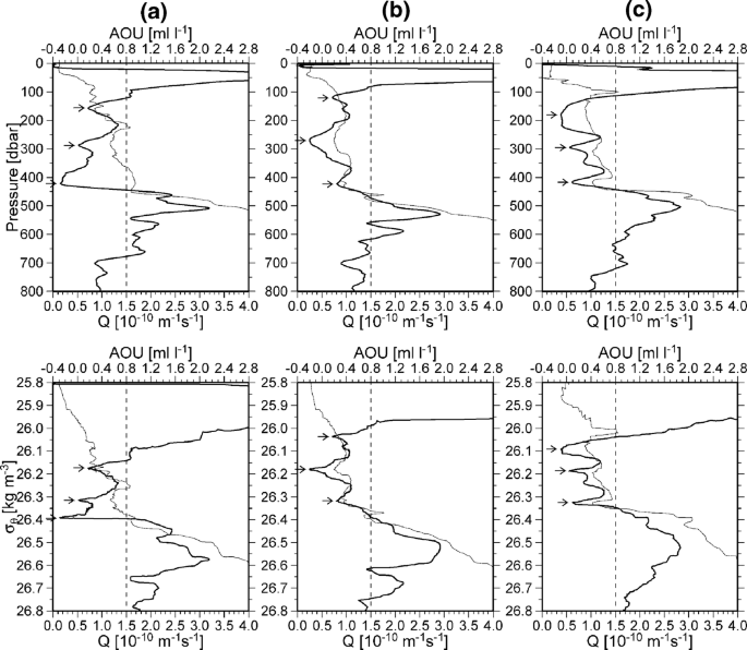
Vertical profiles of Q (thick line) and AOU (thin line) with respect to pressure (upper panel) and σθ (lower panel) obtained by CTDO2 at a 168° E of the 41° N-west section and b 164° E and c 169.17° E of the 37.5° N section, which were near the center of Eddies A, B, and C, respectively. Arrows indicate the cores of a pycnostad. Dashed line in the lower panel represents Q = 1.5 × 10⁻¹⁰ m−1 s−1 and AOU = 0.8 ml l−1 adopted as the threshold for pycnostads and new pycnostads, respectively
Fig. 7 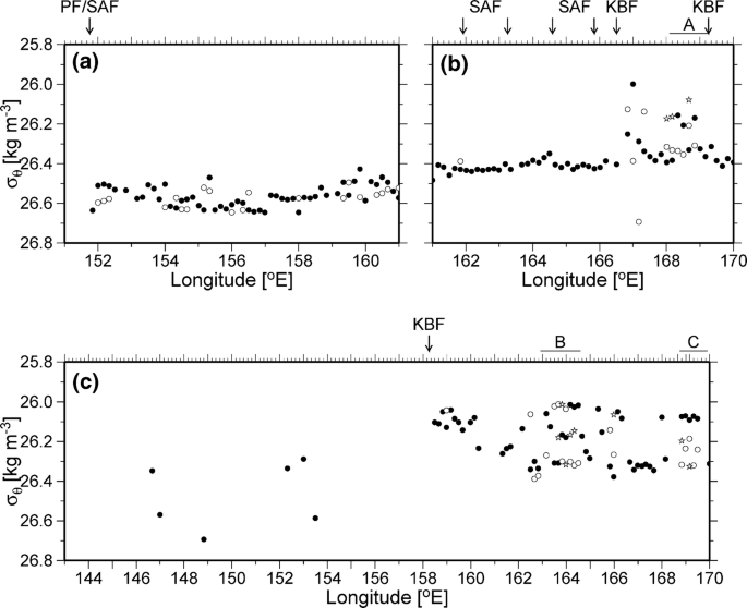
Plots of σθ at the cores of pycnostads against longitude in the a 41° N-west, b 41° N-east, and c 37.5° N sections. Dots, circles, and stars denote the 1st, 2nd, and 3rd cores, respectively. Long (short) ticks, arrows, and horizontal bars on the top of each panel indicate the locations of CTDO2 (XCTD) stations, fronts, and Eddies A–C, respectively
A comparison of dissolve oxygen profiles between this float and the shipboard measurements in our KH-16-3 cruise indicates that the dissolved oxygen from the float had a pressure-dependent negative bias, which yielded a positive AOU bias of ~ 0.2 ml l−1 in the σθ range of 26.0–26.5 kg m−3.


References
Aoyama M, Hamajima Y, Inomata Y, Kumamoto Y, Oka E, Tsubono T, Tsumune D (2018) Radiocaesium derived from TEPCO Fukushima accident in the North Pacific Ocean: surface transport processes until 2017. J Environ Radioact 189:93–102
Belkin I, Krishfield R, Honjo S (2002) Decadal variability of the North Pacific polar front: subsurface warming versus surface cooling. Geophys Res Lett 29:1351
Cui W, Wang W, Zhang J, Yang J (2019) Multicore structures and the splitting and merging of eddies in global oceans from satellite altimeter data. Ocean Sci 15:413–430
Ducet N, Le Traon PY, Reverdin F (2000) Global high-resolution mapping of ocean circulation from TOPEX/Poseidon and ERS-1 and -2. J Geophys Res 105:19477–19498
Favorite F, Dodimead AJ, Nasu K (1976) Oceanography of the Subarctic Pacific region, 1960–1971. Bull Int North Pacific Comm 33:1–187
Gao W, Li P, Xie SP, Xu L, Liu C (2016) Multi-core structure of the North Pacific subtropical mode water from enhanced Argo observations. Geophys Res Lett 43:1249–1255
Goto Y, Yasuda I, Nagasawa M (2018) Comparison of turbulence intensity from CTD-attached and free-fall microstructure profilers. J Atmos Oceanic Tech 35:147–162
Hu W, Murata K, Fukuyama S, Kawai Y, Oka E, Uematsu M, Zhang D (2017) Concentration and viability of airborne bacteria over the Kuroshio Extension region in the northwestern Pacific Ocean: data from three cruises. J Geophys Res Atmos 23:12892–12905
Isoguchi O, Kawamura H, Oka E (2006) Quasi-stationary jets transporting surface warm waters across the transition zone between the subtropical and the subarctic gyres in the North Pacific. J Geophys Res 111:C10003. https://doi.org/10.1029/2005JC003402
Jenkins WJ (1980) Tritium and 3He in the Sargasso Sea. J Mar Res 38:533–569
Joyce TM (1989) On in situ “calibration” of shipboard ADCPs. J Atmos Ocean Technol 6:169–172
Kawai Y, Nishikawa H, Oka E (2019) In situ evidence of low-level atmospheric responses to the Oyashio front in early spring. J Meteorol Soc Jpn 97:423–438
Kouketsu S, Tomita H, Oka E, Hosoda S, Kobayashi T, Sato K (2012) The role of meso-scale eddies in mixed layer deepening and mode water formation in the western North Pacific. J Oceanogr 68:63–77
Levitus S (1982) Climatological atlas of the world ocean. NOAA professional paper 13. In: US Government Printing Office, Washington, DC. p 173
Liu C, Xie SP, Li P, Xu L, Gao W (2017) Climatology and decadal variations in multicore structure of the North Pacific subtropical mode water. J Geophys Res 122:7506–7520
Liu C, Xu L, Xie SP, Li P (2019) Effects of anticyclonic eddies on the multicore structure of the North Pacific subtropical mode water based on Argo observations. J Geophys Res 124:8400–8413
Masuzawa J (1969) Subtropical Mode Water. Deep Sea Res 16:463–472
Mecking S, Warner MJ (2001) On the subsurface CFC maxima in the subtropical North Pacific thermocline and their relation to mode waters and oxygen maxima. J Geophys Res 106:22179–22198
Mitsudera H, Miyama T, Nishigaki H, Nakanowatari T, Nishikawa H, Nakamura T, Wagawa T, Furue R, Fujii Y, Ito S (2018) Low ocean-floor rises regulate subpolar sea surface temperature by forming baroclinic jets. Nat Commun 9:1190
Miyama T, Mitsudera H, Nishigaki H, Furue R (2018) Dynamics of a quasi-stationary jet along the subarctic front in the North Pacific Ocean (the western Isoguchi Jet): an ideal two-layer model. J Phys Oceanogr 48:807–830
Mizuno K, White WB (1983) Annual and interannual variability in the Kuroshio Current System. J Phys Oceanogr 13:1847–1867
Nakamura H (1996) A pycnostad on the bottom of the ventilated portion in the central subtropical North Pacific: its distribution and formation. J Oceanogr 52:171–188
Nakano H, Tsujino H, Sakamoto K, Urakawa S, Toyoda T, Yamanak G (2018) Identification of the fronts from the Kuroshio Extension to the Subarctic Current using absolute dynamic topographies in satellite altimetry products. J Oceanogr 74:393–420
Niiler PP, Maximenko NA, Panteleev GG, Yamagata T, Olson DB (2003) Near-surface dynamical structure of the Kuroshio Extension. J Geophys Res 108:3193
Oka E, Qiu B (2012) Progress of North Pacific mode water research in the past decade. J Oceanogr 68:5–20
Oka E, Suga T (2005) Differential formation and circulation of North Pacific Central Mode Water. J Phys Oceanogr 35:1997–2011
Oka E, Talley LD, Suga T (2007) Temporal variability of winter mixed layer in the mid- to high-latitude North Pacific. J Oceanogr 63:293–307
Oka E, Kouketsu S, Toyama K, Uehara K, Kobayashi T, Hosoda S, Suga T (2011a) Formation and subduction of Central Mode Water based on profiling float data, 2003–2008. J Phys Oceanogr 41:113–129
Oka E, Suga T, Sukigara C, Toyama K, Shimada K, Yoshida J (2011b) “Eddy-resolving” observation of the North Pacific Subtropical Mode Water. J Phys Oceanogr 41:666–681
Oka E, Qiu B, Kouketsu S, Uehara K, Suga T (2012) Decadal seesaw of the central and subtropical mode water formation associated with the Kuroshio Extension variability. J Oceanogr 68:355–360
Oka E, Uehara K, Nakano T, Suga T, Yanagimoto D, Kouketsu S, Itoh S, Katsura S, Talley LD (2014) Synoptic observation of Central Mode Water in its formation region in spring 2003. J Oceanogr 70:521–534
Qiu B, Chen S (2005) Variability of the Kuroshio Extension jet, recirculation gyre and mesoscale eddies on decadal timescales. J Phys Oceanogr 35:2090–2103
Qiu B, Chen S, Hacker P (2007) Effect of mesoscale eddies on subtropical mode water variability from the Kuroshio Extension System Study (KESS). J Phys Oceanogr 37:982–1000
Qiu B, Chen S, Schneider N, Taguchi B (2014) A coupled decadal prediction of the dynamic state of the Kuroshio Extension system. J Clim 27:1751–1764
Riser SC, Freeland HJ, Roemmich D et al (2016) Fifteen years of ocean observations with the global Argo array. Nat Clim Change 6:145–153
Roden GI (1970) Aspects of the mid-Pacific transition zone. J Geophys Res 75:1097–1109
Roden GI (1972) Temperature and salinity fronts at the boundaries of the subarctic-subtropical transition zone in the western Pacific. J Geophys Res 77:7175–7187
Roemmich D, Boebel O, Desaubies Y, Freeland H, King B, LeTraon PY, Molinari R, Owens WB, Riser S, Send U, Takeuchi K, Wijffels S (2001) Argo: the global array of profiling floats. In: Koblinsky CJ, Smith NR (eds) Observing the oceans in the 21st century. Bureau of Meteorology, Melbourne, pp 248–258
Saito H, Suga T, Hanawa K, Watanabe T (2007) New type of pycnostad in the western subtropical-subarctic transition region of the North Pacific: Transition Region Mode Water. J Oceanogr 63:589–600
Saito H, Suga T, Hanawa K, Shikama N (2011) The transition region mode water of the North Pacific and its rapid modification. J Phys Oceanogr 41:1639–1658
Sakurai T, Kurihara Y, Kuragano T (2005) Merged satellite, and in situ data global daily SST. In: Geoscience, and remote sensing symposium, 2005. IGARSS ‘05. Proceedings. (2005) IEEE International, vol 4. Inst Electr Electron Eng, New York, pp 2606–2608
Suga T, Hanawa K, Toba Y (1989) Subtropical mode water in the 137° E section. J Phys Oceanogr 19:1605–1618
Suga T, Takei Y, Hanawa K (1997) Thermostad distribution in the North Pacific subtropical gyre: the central mode water and the subtropical mode water. J Phys Oceanogr 27:140–152
Suga T, Motoki K, Aoki Y, Macdonald AM (2004) The North Pacific climatology of winter mixed layer and mode waters. J Phys Oceanogr 34:3–22
Talley LD (1988) Potential vorticity distribution in the North Pacific. J Phys Oceanogr 18:89–106
Talley LD, Raymer ME (1982) Eighteen degree water variability. J Mar Res 40:757–775
Taneda T, Suga T, Hanawa K (2000) Subtropical mode water variation in the southwestern part of the North Pacific subtropical gyre. J Geophys Res 105:19591–19598
Tomosada A (1986) Generation and decay of Kuroshio warm-core rings. Deep Sea Res 33:1475–1486
Tsujino H, Yasuda T (2004) Formation and circulation of mode waters of the North Pacific in a high-resolution GCM. J Phys Oceanogr 34:399–415
Wagawa T, Ito S, Shimizu Y, Kakehi S, Ambe D (2014) Currents associated with the quasi-stationary jet separated from the Kuroshio Extension. J Phys Oceanogr 44:1636–1653
Yasuda I (2003) Hydrographic structure and variability of the Kuroshio–Oyashio transition area. J Oceanogr 59:389–402
Yasuda I, Okuda K, Hirai M (1992) Evolution of a Kuroshio warm-core ring—variability of the hydrographic structure. Deep Sea Res 39:S131–S161
Yuan X, Talley LD (1996) The subarctic frontal zone in the North Pacific: characteristics of frontal structure from climatological data and synoptic surveys. J Geophys Res 101:16491–16508
Acknowledgements
The authors are grateful to the captain, crew, and scientists participating in the KH-13-3 and KH-16-3 cruises of the R/V Hakuho-maru of the Japan Agency for Marine-Earth Science and Technology for their efforts in conducting the CTDO2 and XCTD measurements. They also thank Shigeki Hosoda and Kanako Sato for their assistance in processing the Argo float data and Shuiming Chen, Yutaka Yoshikawa, and two anonymous reviewers for their helpful comments. This study was conducted in JFY2019 when EO and SS were staying at the International Pacific Research Center (IPRC), University of Hawaii at Manoa for their sabbatical, under the Tohoku University 2019 Leading Young Researcher Overseas Visit Program (for SS). EO and SS thank Kelvin Richards and Niklas Schneider (former and current Directors of IPRC), Atsushi Tsuda and Tomohiko Kawamura (former and current Directors of Atmosphere and Ocean Research Institute, the University of Tokyo), Ryota Hino (Chair of the Department of Geophysics, Tohoku University), and Toshio Suga (Director of the International Joint Graduate Program in Earth and Environment Sciences, Tohoku University). This study is supported by the Japan Society for Promotion of Science (KAKENHI, Grant-in-Aid for Scientific Research (B) nos. 21340133 and 25287118 and (C) no. 17K05652, and Grant-in-Aid for Scientific Research on Innovative Areas under Grant nos. 22106007 and 19H05700).
Author information
Authors and Affiliations
Corresponding author
Rights and permissions
Open Access This article is licensed under a Creative Commons Attribution 4.0 International License, which permits use, sharing, adaptation, distribution and reproduction in any medium or format, as long as you give appropriate credit to the original author(s) and the source, provide a link to the Creative Commons licence, and indicate if changes were made. The images or other third party material in this article are included in the article's Creative Commons licence, unless indicated otherwise in a credit line to the material. If material is not included in the article's Creative Commons licence and your intended use is not permitted by statutory regulation or exceeds the permitted use, you will need to obtain permission directly from the copyright holder. To view a copy of this licence, visit http://creativecommons.org/licenses/by/4.0/.
About this article

Cite this article
Oka, E., Kouketsu, S., Yanagimoto, D. et al. Formation of Central Mode Water based on two zonal hydrographic sections in spring 2013 and 2016. J Oceanogr 76, 373–388 (2020). https://doi.org/10.1007/s10872-020-00551-9
Received:
Revised:
Accepted:
Published:
Issue Date:
DOI: https://doi.org/10.1007/s10872-020-00551-9