
Abstract
We study the optimal tax/pension design in a two-period model where individuals differ in both productivity and discount rates or projection bias and where their utility of the retirement period consumption is not independent of the earlier standard of living. We consider both welfarist and paternalistic social objectives. The paternalistic government attempts to correct the projection bias by using a higher discount factor. We derive general mathematical expressions that characterize optimal tax/pension design (marginal tax/subsidy rates). They suggest that the pattern of marginal labor income taxes depends on habit formation. Negative marginal labor income tax rates are possible. To gain a better understanding, we examine numerically the properties of an optimal lifetime redistribution policy with habit formation. We find support for non-linear tax/pension program in which some types of individuals are taxed while some are subsidized. The effect of changes in the degree of habit formation is explored in the numerical simulations as well as the implications of different degrees of correlation between skill and projection bias.


Notes
Diamond (1977) discussed the case where individuals may under-save due to mistakes. He concluded that if there were not mandatory pension program, a substantial part of population would not have adequate savings for retirement. Feldstein (1985) studied the optimal pay-as-you-go system in an OLG setting in a case where individuals have higher discount rates than the government. In a model with inelastic labor supply and no uncertainty he finds that social security system ensuring retirement income is either not optimal at all or should have very low replacement rate. İmrohoroğlu et al. (2003) made numerical simulations in a pay-as-you-go model when individuals have hyperbolic discounting preferences. Diamond and Kőszegi (2003) also employ this kind of model with hyperbolic discounting to study the policy effects of endogenous retirement choices using a public pension system as a commitment device. Market-based commitment devices, such as long-term saving contracts, work only for those who are aware of their lack of commitment, see e.g. Laibson et al. (1998), Choi et al. (2003), Haveman et al. (2007), Benartzi and Thaler (2007).
Loewenstein et al. (2003) present a survey of some empirical evidence on the presence of projection bias. People tend to underappreciate the adaptation to the change in the standard of living, i.e. changes in their long-term preferences.
Discount factor (rates), time preferences and projection bias refer to the same phenomenon, the level of appreciation of future consumption, in this paper.
\(\delta= \frac{1}{1 + \xi}\) where ξ is discount rate or a parameter describing time preference.
The idea can be clarified as follows: assume that δ′ is the actual, common discount factor, but individuals believe that their discount factor is δ=β ∗ δ′, where β∈[0,1] reflects the level of projection bias and β varies between types.
Non-separability of utilities in each period would already alone imply habit formation, but we have chosen to use parameter ρ to make the effect of habit formation clearer.
Another case, where some of the individuals over-save, i.e. use too high discount factor to maximize their lifetime utility, can also easily be analyzed with the same framework. Similarly, the case where government uses the same discount factor as those suffering less from projection bias can be obtained as a special case of the analysis presented here. In this paper, however, we concentrate on a case where all individuals suffer from projection bias and under-save as a result of it.
See Appendix A for derivation.
This is in line with the result in the context of second-best environmental taxation (see Pirttilä and Tuomala 1997).
See for example Cremer et al. (2009) for a similar approach.
See Appendix A.
The marginal implicit tax rate for savings chosen by the government, α, takes care of the negative internality, whereas an individual, doing labor supply and savings choices, sees that as a pure distortion. From the perspective of the individual the distortion is still given by d. From a similar term as in the welfarist case, (12a)–(12d), we get the distortions from the individuals’ perspectives.
$$ \sigma^{i} = \frac{1}{r}\biggl[ 1 - \frac{u_{c}}{\lambda N^{i}}\biggl( \sum_{j} \mu^{ji} \Delta^{ji} - N^{i}\Delta^{gi} \biggr) \biggr] $$(∗)where \(\Delta^{ji} = \frac{\delta^{j} - \delta^{i}}{\delta^{i}}\) and \(\Delta^{gi} = \frac{\delta^{g} - \delta ^{i}}{\delta^{i}}\).
Compared to the welfarist case there now appears an additional term N iΔgi in (∗) that results from the difference in the discount factors between the government and individuals. This can be called a Pigovian term. When all μ’s are zero we are in the first-best situation.
Due to the bunching the marginal tax rates on labor income are equal for types 1 and 2.
The result is not uncommon for a model with paternalistic objectives and multidimensional self-selection constraints. A similar result is found e.g. in Cremer et al. (2009).
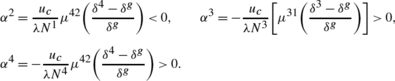
Other formulas for the marginal tax rate on labor income are
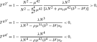
and for the marginal tax rates on savings, are
To reach reliable quantitative results, a general equilibrium approach would be more suitable. However, introducing endogenous wages and interest rate would require a more sophisticated simulation model, and it is left for future challenge.
By downward and upward binding self-selection constraints we refer here to our numbering. As the numbering is chosen here more or less randomly, it is important not to make the assumptions of the reduced-form optimization before checking the actual pattern of binding constraints.
The only exception was the extreme case where types 1 and 3 suffered from full myopia. In the case with myopia, the same three constraints (red arrows in Table 3) are still binding, but the constraints between types 1 and 2 are now genuinely binding, and, in addition to that, the constraint stopping patient high-skilled from mimicking the impatient high-skilled binds.
For example, in the Finnish pension system replacement rates for wage earners vary mainly between 55 and 70 per cent.
The Gini coefficient is interpreted here purely as a descriptive measure. It also has a normative interpretation. The social value of income declining according to a person’s rank in the distribution is the weighting underlying the Gini coefficient (see Sen 1974).
When the level of habit formation exceeds this level, it is not easy to find solutions in our example. Moreover, very high levels of habit formation would imply that the second period utility would mainly consist of the working period consumption, which we find implausible. The values between 0 and 0.7 are the most reasonable values for the weight of the previous consumption.
Not surprisingly labor supply increases with the degree of habit formation (Fig. 2). This result holds for all the types.
Note \(\delta= \frac{1}{1 + \xi}\), where ξ is discount rate or time preference.


References
Akerlof, G. A. (1978). The economics of “tagging” as applied to the optimal income tax, welfare programs and manpower planning. American Economic Review, 68, 8–19.
Akerlof, G. (2002). Behavioral macroeconomics and macroeconomic behavior. American Economic Review, 92(3), 411–433.
Benartzi, S., & Thaler, R. (2007). Heuristics and biases in retirement savings behaviour. Journal of Economic Perspectives, 21, 81–104.
Boadway, R., Marchand, M., Pestieau, P., & del Mar Racionero, M. (2002). Optimal redistribution with heterogeneous preferences for leisure. Journal of Public Economic Theory, 4, 475–498.
Blomquist, S., & Christiansen, V. (2004). Taxation and heterogeneous preferences. CESifo working paper 1244.
Choi, J., Laibson, D., Madriand, B., & Metrick, A. (2003). Optimal defaults. American Economic Review Papers and Proceedings, 93, 180–185.
Cremer, H., Pestieau, P., & Rochet, J.-C. (2001). Direct versus indirect taxation: the design of the tax structure revisited. International Economic Review, 42, 781–799.
Cremer, H., De Donder, P., Maldonado, D., & Pestieau, P. (2008). Habit formation and labor supply. CESifo Working Paper No. 2351.
Cremer, H., De Donder, P., Maldonado, D., & Pestieau, P. (2009). Forced saving, redistribution and non-linear social security scheme. Southern Economic Journal, 76(1), 86–98.
Cuff, K. (2000). Optimality of workfare with heterogeneous preferences. Canadian Journal of Economics, 33, 149–174.
Diamond, P. A. (1977). A framework for social security analysis. Journal of Public Economics, 8, 275–298.
Diamond, P. A. (2003). Taxation, incomplete markets, and social security. The 2000 Munich Lectures. Cambridge: MIT Press.
Diamond, P. A., & Kőszegi, B. (2003). Quasi-hyperbolic discounting and retirement. Journal of Public Economics, 87, 1839–1872.
Diamond, P. A., & Mirrlees, J. (2000). Adjusting one’s standard of living: two period models. In P. J. Hammond & G. D. Myles (Eds.), Incentives, organization and public economics, papers in honour of Sir James Mirrlees (pp. 107–122). Oxford: Oxford University Press.
Diamond, P. A., & Spinnewijn, J. (2009). Capital income taxes with heterogeneous discount rates. NBER Working paper 15115.
Duesenberry, J. S. (1949). Income, saving and the theory of consumer behaviour. Cambridge: Harvard University Press.
Feldstein, M. (1985). The optimal level of social security benefits. Quarterly Journal of Economics, 100(2), 300–320.
Haveman, R., Holden, K., Romanov, A., & Wolfe, B. (2007). Assessing the maintenance of savings sufficiency over the first decade of retirement. International Tax and Public Finance, 14(4), 481–502.
İmrohoroğlu, A., İmrohoroğlu, S., & Joines, D. H. (2003). Time inconsistent preferences and social security. Quarterly Journal of Economics, 118(2), 745–784.
Judd, K. L., & Su, C.-L. (2006). Optimal income taxation with multidimensional taxpayers types. Computing in economics and finance 2006 (Vol. 471). Society for Computational Economics.
Laibson, D., Repetto, A., & Tobacman, J. (1998). Self-control and saving for retirement. Brookings Papers on Economic Activity, 1, 91–196.
Loewenstein, G., O’Donoghue, T., & Rabin, M. (2003). Projection bias in predicting future utility. Quarterly Journal of Economics, 118(4), 1209–1248.
Mirrlees, J. (1971). An exploration in the theory of optimum income taxation. Review of Economic Studies, 38, 175–208.
Pirttilä, J., & Tuomala, M. (1997). Income tax, commodity tax and environmental policy. International Tax and Public Finance, 4, 379–393.
Pollak, R. (1970). Habit formation and dynamic demand functions. Journal of Political Economy, 78(4), 745–763.
Ryder, H., & Heal, G. (1973). Optimal growth with intertemporally dependent preferences. Review of Economic Studies, 40, 1–33.
Sandmo, A. (1993). Optimal redistribution when tastes differ. Finanzarchiv, 50(2), 149–163.
Sen, A. (1974). Informational bases of alternative welfare approaches: aggregation and income distribution. Journal of Public Economics, 3(4), 387–403.
Tarkiainen, R., & Tuomala, M. (1999). Optimal nonlinear income taxation with a two-dimensional population: a computational approach. Computational Economics, 13, 1–16.
Tarkiainen, R., & Tuomala, M. (2007). On optimal income taxation with heterogeneous work preferences. International Journal of Economic Theory, 3, 35–46.
Tenhunen, S., & Tuomala, M. (2010). On optimal lifetime redistribution policy. Journal of Public Economic Theory, 12(1), 171–198.
Author information
Authors and Affiliations
Corresponding author
Appendices
Appendix A: Derivations of implicit taxes on savings
1.1 A.1 Derivation of (12a)–(12d)
Step 1: To rewrite the marginal rate of substitution \(\frac {u_{c} + \delta^{i}\rho v_{c}}{\delta^{i}v_{x}}\) with help of the first order conditions, we first solve the numerator from (5). By adding and subtracting a term ∑ j μ ji δ i ρv c the first order condition with respect to c given in (5) can be written as

From this we can solve
Similarly we solve for the denominator of the marginal rate of substation. By adding and subtracting the term ∑ j μ ji δ i v x to the first order condition with respect to x given in (6), it can be written as
From this we can solve
By combining (21) and (22) and making use of definition of the proportional difference in discount rates, \(\Delta^{ji} = \frac {\delta ^{j} - \delta^{i}}{\delta^{i}}\), we can write
Step 2: Manipulating equation to a useful form
The next trick is to multiply the both sides of (25) by term \(\frac{\lambda N^{i}r + \delta^{i}\sum_{j} \mu^{ji}\Delta ^{ji}v_{x}}{ \delta^{i}\sum_{j} \mu^{ji}\Delta^{ji}v_{x}}\) . This gives us
Rearranging terms gives us
With this form we can solve for the marginal rate of substitution, \(\frac{u_{c} + \delta^{i}\rho v_{c}}{\delta^{i}v_{x}}\), in a form given in (12a)–(12d).
1.2 A.2 Derivation of (20)
Paternalistic case follows a similar procedure as in a welfarist case, so details of the derivations are omitted. The terms to be added and subtracted to first order conditions are now ∑ j μ ij δ g ρv c −∑ j μ ji δ g ρv c and ∑ j μ ij δ g v x −∑ j μ ji δ g v x . The term that is used to multiply equation in step 2 is
1.3 A.3 Derivation of (∗) in Footnote 15
Derivation proceeds similarly to the earlier cases. The terms to be added and subtracted to the first order conditions are N i δ i ρv c −∑ j μ ji δ i ρv c and N i δ i v x −∑ j μ ji δ i v x . In step 2, the multiplier to be used is
Appendix B: Numerical simulations
2.1 B.1 Procedure
Numerical simulation was carried out with the Matlab program. The function used (fmincon) solves the optimum of a multivariable function with equality and inequality constraints that may be linear or non-linear. It also determines which of the constraints are binding. The same procedure is applied to all cases considered in this paper.
Note that as the optimization function also allowed slack constraints, we were not restricted to a priori assumptions on the binding self-selection constraints. Thus, we included all possible constraints in the optimization procedure and simply determined the binding constraints with the help of numerical solutions.
Multidimensional screening problems are numerically challenging to solve, as discussed in Judd and Su (2006). We also encountered some difficulties with the solvability of the problem, as the matrix including the constraints with opposite self-selection constraints is very close to being singular. These difficulties were met during the sensitivity analysis; with some combinations of parameters the problem was not solvable or gave irrational values.
2.2 B.2 Parameterization
The distribution of the economy was chosen to be uniform merely for the simplicity and comparability for the following cases. The discount factors, δ L and δ H, were set as 0.6 and 0.8, while δ g was set equal to 1. These values are in line with e.g. Cremer et al. (2009) who performed similar numerical calculations. The wage rates reflecting the productivities were chosen to be 2 and 3, respectively. The magnitude of the wage rates was determined by the solvability of the problem; with these wage rates, the labor supply decisions, restricted to lie between 0 and 1, were at reasonable levels.

2.3 B.3 Sensitivity analysis
We have considered the sensitivity of the analysis with the help of varying (i) the degree of habit formation, which allows us to compare the cases with and without habit effect, and (ii) the correlation between the characteristics of the individuals, skill level and discount factor. With the some combinations of the parameters there is a failure to find the optimum, but it is due to technical problems in the optimization algorithm.
The first part, sensitivity with respect to degree of habit formation, is presented in the main text. The results considering sensitivity with respect to correlation between the two unobservable features follow here.
Rights and permissions
About this article
Cite this article
Tuomala, M., Tenhunen, S. On the design of an optimal non-linear tax/pension system with habit formation. Int Tax Public Finance 20, 485–512 (2013). https://doi.org/10.1007/s10797-012-9239-7
Published:
Issue Date:
DOI: https://doi.org/10.1007/s10797-012-9239-7