Formal Model of Business Processes Integrated with Business Rules

Kluza, Krzysztof; Nalepa, Grzegorz J.

doi:10.1007/s10796-018-9826-y

Formal Model of Business Processes Integrated with Business Rules

Open access
Published: 19 February 2018

Volume 21, pages 1167–1185, (2019)
Cite this article

Download PDF

You have full access to this open access article

Information Systems Frontiers Aims and scope Submit manuscript

Formal Model of Business Processes Integrated with Business Rules

Download PDF

3964 Accesses
11 Citations
Explore all metrics

Abstract

Business Processes describe the ways in which operations are carried out in order to accomplish the intended objectives of organizations. A process can be depicted using a modeling notation, such as Business Process Model and Notation. Process model can also describe operational aspects of every task; but in a properly designed model, the detailed aspects of low-level logic should be delegated to external services, especially to a Business Rule Engine. Business Rules support the specification of knowledge in a declarative manner and can be successfully used for specification of details for process tasks and events. However, there is no unified model of process integrated with rules that ensures data types consistency. Thus, the paper presents a formal description of the integration of Business Processes with Business Rules. We provide a general model for such integration as well as the model applied to a specific rule representation from the Semantic Knowledge Engineering approach.

Coordinating Decision-Making in Data Management Activities: A Systematic Review of Data Governance Principles

Monitoring the GDPR

Solving business problems: the business-driven data-supported process

Article 06 January 2024

1 Introduction

Business Process Management (BPM) (Dumas et al. 2013; Weske 2012) is a holistic approach for improving organization’s workflow in order to align processes with client needs. It focuses on reengineering of processes to obtain optimization of procedures, increase efficiency and effectiveness by the constant process improvement.

According to this approach, a Business Process (BP) can be simply defined as a collection of related tasks which produces a specific service or product for a customer (Lindsay et al. 2003). Models of BPs are intended to be a bridge between technical and business people. They are simple and visualizations make them much easier to understand than using a textual description. Thus, modeling is an essential part of BPM.

Although processes provide a universal method of describing operational aspects of business, detailed aspects of process logic should be described on different abstraction level. Business Rules (BR) can be successfully used to specify process low-level logic (Charfi and Mezini 2004; Knolmayer et al. 2000). What is important, the BR approach supports the specification of knowledge in a declarative manner.

There is a difference in abstraction levels of BP and BR; however, rules can be to a certain degree complementary to processes. BR provide a declarative specification of domain knowledge, which can be encoded into a process model (Kluza et al. 2012). On the other hand, a process can be used as a procedural specification of the workflow, including the inference control.

The use of BR in BP design helps to simplify complex decision modeling. It was also empirically proven that the effect of linked rules improved business process model understanding (better time efficiency in interpreting business operations, less mental effort, improved accuracy of understanding) (Wang et al. 2017). Although rules should describe business knowledge in a formalized way that can be further automated (Nalepa and Ligęza 2005), there is no common understanding how process and rule models should be structured in order to be integrated (Hohwiller et al. 2011). There is also no formalized model that combines processes with rules and ensures data types consistency, i.e. data types used in rules should be available in processes that use these rules. This is the main challenge we wish to address in our work.

As a solution, to the above mentioned challenge, we propose a model for describing integration of BP with BR. Our starting point are some existing representation methods for processes and rules, specifically Business Process Model and Notation (BPMN) (OMG 2011a) for BP models, and eXtended Tabular Trees version 2 (XTT2) (Nalepa et al. 2011c) which is a formalized rule representation developed as a part of the Semantic Knowledge Engineering (SKE) approach (Nalepa 2011). We extend these models, and on top of them provide a formalized general business logic model that incorporates rules in the process models. The model uses the abstract rule representation, so it can be refined by adjusting it to the specific rule representation. In the paper, we use XTT2 for this purpose, as it is a fully formalized rule representation. In our case, the proposed model deals with the integration of processes with rules to provide a coherent formal description of the integrated model.

Usually, the goal of formal model description is its formal verification. In our case, the proposed model deals with the integration of processes with rules to provide a coherent formal description of the integrated model. Although we do not consider the formal verification of such a model, as we take advantage of the existing representations, the formal verification of each part of the integrated model (process or rules) is possible. Because of using the XTT2 rule representation, it is possible to use the existing methods for formal verification of rules (Ligęza 1999), especially for formal verification of decision components, such as inconsistency, completeness, subsumption or equivalence (Nalepa et al. 2011a). In the case of process model itself, one can use the existing verification methods (Wynn et al. 2009), specifically the methods that can take into account the task logic (Szpyrka et al. 2011).

The paper is organized as follows. Section 2 presents an overview of related works concerning process model formalization. Section 3 provides a formal description of a BPMN process model. It introduces the notation and its formal representation. This formalized process model is then integrated with rules, and this integration is specified as the General Business Logic Model in Section 4. In order to apply this model to a specific rule solution, the SKE-specific Business Logic Model is presented in Section 5. As an evaluation, a case example described using the proposed model is presented in Section 6. The paper is concluded in Section 7.

2 Related Works

There are several attempts to the formalization of Business Process models. These formalizations differ with respect to the goal with which the model semantics is specified.

2.1 Formalization of Business Process Models

Ouyang et al. (2006a, b) introduced a formal description of BPMN process model for the purpose of their translation to Business Process Execution Language (BPEL), in order to execute process models. They also defined the concept of well-structured components for the purpose of the execution. Dijkman et al. (2007) defined the formal semantics of BPMN process model in order to use formal analysis. The main goal of their formalization was to define the execution semantics to enable soundness checking. In Dijkman and Gorp (2011), they formalized execution semantics of BPMN through translation to Graph Rewrite Rules. Such formalization can support simulation, animation and execution of BPMN 2.0 models. It can help in conformance testing of implementations of the workflow engines that use the notation for modeling and executing processes.

In 2002, Sivaraman and Kamath (2002) used Petri nets for modeling Business Processes. However, it was before the BPMN notation was introduced. In fact, the translation from BPMN to Petri nets is not straightforward. Changizi et al. (2010) formalized BP model through translation to channel-based coordination language Reo. Such transformations allows for verification of models with the help of verification and model checking tools available for the Reo language, such as mCRL2 model checker. Speck et al. (2011) formalized Event-driven Process Chain (EPC) diagrams using Computational Tree Logic (CTL). With CTL, it is possible to formulate rules about different paths in processes and use that for checking the existence of a specific element type in the process, for unknown elements or elements with only partially known properties. Wong and Gibbons (2008, 2011) defined BPMN model semantics in terms of the Z model for syntax and Communicating Sequential Processes (CSP) for behavioral semantics. This allows for checking the consistency of models at different levels of abstraction as well as other properties that must apply to the process, such as domain specific properties, deadlock-freeness or proper completion.

Lam (2009, 2012) formally defined the token-based semantics of BPMN models in terms of Linear Temporal Logic (LTL). This allows for verification and reasoning on BPMN models, especially for checking such properties as liveness or reachability. Ligęza (2011) defined a declarative model for well-defined BPMN diagrams, which allows for specification of correct components and correct dataflow, especially checking model consistency or termination condition. Smirnov et al. (2012) introduced simple formalization for defining action patterns in business process model repositories. Action patterns capture different relations among actions often observed within process model collections. The formalization used in Smirnov et al. (2012) allowed the authors extract various types of action patterns from industrial process model collections.

Bădică et al. (2003) presented the method for modeling business processes using Role Activity Diagrams which share many similarities with BPMN. They used the formalization that exploits Finite State Process Algebra (FSP) which is suitable for verification of these models using Fluent Linear Temporal Logic (FLTL) (Bădică and Bădică 2011).

2.2 Decision Model and Notation and Business Process Models

On the other hand, there is a new standard for modeling decisions of organizations – Decision Model and Notation (DMN) (OMG 2015). The DMN specification shows examples how to link decisions in business process with specific elements in the process model. However, it does not specify the details of this relationship. Moreover, it emphasizes the independence of the DMN of the business process and BPMN. The handbook for process and decision modeling (Debevoise et al. 2014) presents how to separate decision logic to DMN during modeling, but it does not specify the formal relationships between the models and their integration issues.

Janssens et al. (2016) specified five integration scenarios of decision and processes, which covers the continuum from processes without decisions (scenario 0) to decisions without processes (scenario 4). Our approach can be located somewhere between scenario 1, in which local decisions ensure separation of control flow and decision logic, and scenario 2, where decisions are placed directly before the business activities requiring their output. This paper systematize the integration possibilities, but it does not consider the data integration between models.

Batoulis et al. (2015b) proposed a method for extracting decision logic from process models. They specified three patterns for control-flow-based decision identification and provide an algorithm for transforming such decision logic to DMN model. This is suitable for refactoring process models in order to separate decision logic from process models. Bazhenova and Weske (2015) proposed an approach for deriving decision models from process models and execution logs. The approach consists of four steps: decision points identification, decision logic finding, constructing decision model and adapting process model. Thus, it requires the event log of a process model. Another approach which dynamically adapts the decision logic based on historic and current process execution data in BPM system during run-time was proposed in Batoulis et al. (2015a). In this approach, the decisions are automatically revealed and translated to DMN what improves process executions regarding such issues as process duration or costs. Catalkaya et al. (2013) proposed the method for applying decision theory to process models and extend the current standard with rule-based XOR-split gateway (the so called r-gateway). In order to take a decision the method utilize key performance indicators, such as cost of performing an activity.

It is important to emphasize that DMN relation to BPMN is described in the “Annex A: Relation to BPMN” of the DMN specification (OMG 2015) only in the informative way. Linking BPMN and DMN Models is described informally. Thus, no constraints or requirements for data are imposed.

The formalizations mentioned above were used either for formal analysis of the model (checking selected properties) or its execution. In the case of the DMN representation, there are research directions providing the way of deriving decision models from process models and describing the possibility of execution of such models. However, in the approach presented in this paper, we focus on designing the integrated models, so the purpose of the model is to formally describe the integration of the BP model with rules and to provide the basis for the formal description of other integration issues. It is partially based on the BPMN formalization proposed by Ouyang et al. (2006a). Yet we extend this formalization by incorporating rules into process models, which is our original contribution.

3 Formal Description of BPMN Process Model

Let us define a BPMN 2.0 process model that describes the most important artifacts of the BPMN notation.^{Footnote 1} As it focuses also on several details that are key elements from the rule perspective, the process model takes into account flow objects (activities, events and gateways), sequence flows between these flow objects, as well as the set of model attributes.

Definition 1

A BPMN 2.0 process model is a tuple $\mathcal {P} = (\mathcal {O}, \mathcal {F}, {\Lambda })$, where:

$\mathcal {O}$ is the set of flow objects, $o_{\mathit {1}},o_{\mathit {2}},o_{\mathit {3}},\ldots \in \mathcal {O}$,
Λ is the set of model attributes, λ₁,λ₂,λ₃,… ∈Λ,
$\mathcal {F} \subset \mathcal {O} \times \mathcal {O} \times 2^{{\Lambda }_{\mathcal {F}}}$ is the set of sequence flows, where ${\Lambda }_{\mathcal {F}} \subset {\Lambda }$ is a subset of attributes that are used in sequence flows.

Moreover, the set of flow objects is divided into sets:

$\mathcal {A}$ is the set of activities such that $\mathcal {A} = \mathcal {T} \cup \mathcal {S}$, $\mathcal {T} \cap \mathcal {S} = \emptyset $, where $\mathcal {T}$ is the set of tasks and $\mathcal {S}$ is the set of sub-processes, $\tau _{\mathit {1}},\tau _{\mathit {2}},\tau _{\mathit {3}},\ldots \in \mathcal {T}$ and $s_{\mathit {1}},s_{\mathit {2}},s_{\mathit {3}},\ldots \in \mathcal {S}$,
$\mathcal {E}$ is the set of events, $e_{\mathit {1}},e_{\mathit {2}},e_{\mathit {3}},\ldots \in \mathcal {E}$
$\mathcal {G}$ is the set of gateways, $g_{\mathit {1}},g_{\mathit {2}},g_{\mathit {3}},{\ldots } \in \mathcal {G}$

such that $\mathcal {O} = \mathcal {A} \cup \mathcal {E} \cup \mathcal {G}$ and $\mathcal {A} \cap \mathcal {E} = \mathcal {A} \cap \mathcal {G} = \mathcal {E} \cap \mathcal {G} = \emptyset $.

The set of all the possible BPMN 2.0 process models will be denoted $\boldsymbol {\mathcal {P}}$, e.g. $\mathcal {P}_{\mathit {1}}, \mathcal {P}_{\mathit {2}}, \mathcal {P}_{\mathit {3}},{\ldots } \in \boldsymbol {\mathcal {P}}$.

Definition 2

A task interpretation is a pair:

$$\tau = (\mathit{type}(\tau),{\Lambda}_{\tau}) $$

where:

type(τ) determines the type of the task τ, type(τ) ∈{None, User, Manual, Send, Receive, Script, Service, BusinessRule}
Λ_τ ⊂Λ is the set of the task attributes, Λ_τ = {id, name, documentation, markers, resources,…, implementation},^{Footnote 2} some attributes can take set values, such as:
- markers ⊂{loop, parallelMI, sequentialMI, adhoc, compensation},
some of the attributes may contain other attributes, such as:
- ioSpecification = {dataInputs,dataOutputs}.

Moreover, $\mathcal {T}_{x}$ will denote the set of tasks of the same type x:

$$\mathcal{T}_{x} = \{ \tau \in \mathcal{T}\colon \mathit{type}(\tau) = x \} $$

For simplicity, the value of an attribute can be obtained using a function, name of which matches the attribute name attribute(τ), e.g. id(τ₁) denotes the value of the id attribute for the task τ₁.

The tasks of different type use the implementation attribute to specify the implementation technology, e.g. “##WebService” for the Web service technology or a URI identifying any other technology or coordination protocol. The purpose of the implementation technology is different for different types of tasks, e.g.: in the case of Service tasks ($\mathcal {T}_{\mathit {Service}}$) it determines the service technology, in the case of Send tasks ($\mathcal {T}_{\mathit {Send}}$) or Receive tasks ($\mathcal {T}_{\mathit {Receive}}$), it specifies the technology that will be used to send or receive messages respectively, and in the case of Business Rule tasks ($\mathcal {T}_{\mathit {Business~Rule}}$), it specifies the Business Rules Engine technology. The ioSpecification attribute is used for specifying the data inputs and outputs suitable for the implementation technology. Some types of tasks can also have several additional attributes (Λ_τ) specified.

Definition 3

A sub-process interpretation is a triple:

$$s = (\mathcal{P}_{s}, \mathit{type}(s),{\Lambda}_{s}) $$

where:

type(s) determines the type of the sub-process s, type(s) ∈{Sub-process,Embedded,CallActivity,Transaction,Event},
$\mathcal {P}_{s} \in \boldsymbol {\mathcal {P}}$ is a BPMN 2.0 process model nested in the sub-process s,
Λ_s ⊂Λ is the set of the sub-process attributes, Λ_τ = {id,name,documentation,markers,…,triggeredByEvent},^{Footnote 3} such attributes are defined same as for tasks (see Definition 2).

While activities represent parts of work that are performed within a Business Process, events are state changes occurring in the process environment that can influence the process.

Definition 4

An event interpretation is a pair:

$$e = (\mathit{type}(e),\mathit{trigger}(e),{\Lambda}_{e}) $$

where:

type(e) ∈{Start,Intermediate,End},
trigger(e) determines the trigger of the event e, trigger(e) ∈{Cancel, Compensation, Conditional, Error, Escalation, Link, Message, Multiple, None, ParallelMultiple,Signal,Terminate,Timer},
Λ_e ⊂Λ is the set of the event attributes, Λ_e = {id, name, documentation, method, boundary, attachedToRef, cancelActivity},^{Footnote 4}method(e) ∈{catch,throw}.

Moreover, $\mathcal {E}^{x}$ will denote the set of events with the same trigger x:

$$\mathcal{E}^{x} = \{ e \in \mathcal{E}\colon \mathit{trigger}(e) = x \} $$

$\mathcal {E}_{x}$ will denote the set of events of the same type x:

$$\mathcal{E}_{x} = \{ e \in \mathcal{E}\colon \mathit{type}(e) = x \} $$

Different types of events have different event definition attributes specified, e.g.:

messageEventDefinition for $e \in \mathcal {E}^{\mathit {Message}}$, messageEventDefinition = {messageRef,operationRef},
timerEventDefinition for $e \in \mathcal {E}^{\mathit {Timer}}$, timerEventDefinition = {timeCycle,timeDate,timeDuration},
conditionalEventDefinition for $e \in \mathcal {E}^{\mathit {Conditional}}$, conditionalEventDefinition = {condition},

It is also important to note that not every trigger(e) is allowed for any type(e) of event – Table 1 presents the possible combinations.

Table 1 Possible combinations of trigger(e) and type(e)

Full size table

In the case of this formalization, the condition attribute for $e \in \mathcal {E}^{\mathit {Conditional}}$ is especially important. It defines an expression stored in body attribute and expressed in the language language: condition(e) = {body(e),language(e)}.

Gateway elements are used to control the flow of tokens through sequence flows as they converge and diverge within a process. Although, according to the BPMN 2.0 specification, a single gateway can have multiple input and multiple output flows, this formalized model proposed is to enforce a best practice of a gateway only performing one of these functions. Thus, a gateway should have either one input or one output flow and a gateway with multiple input and output flows should be modeled with two sequential gateways, the first of which converges and the second diverges the sequence flows.

Definition 5

A gateway interpretation is a tuple:

$$g = (\mathcal{F}_{g}^{in},\mathcal{F}_{g}^{out},\mathit{type}(g),{\Lambda}_{g}) $$

where:

${\mathcal {F}}_{g}^{in}$ and ${\mathcal {F}}_{g}^{out}$ are sets of sequence flows (input and output flows respectively), ${\mathcal {F}}_{g}^{in}$, ${\mathcal {F}}_{g}^{out} \subset \mathcal {F}$, ${\mathcal {F}}_{g}^{in} = \{ (o_{\mathit {i}},o_{\mathit {j}},{\Lambda }_{i,j}) \in \mathcal {F}\colon o_{\mathit {j}} = g\}$ and ${\mathcal {F}}_{g}^{out} = \{ (o_{\mathit {i}}, o_{\mathit {j}}, {\Lambda }_{i,j}) \in \mathcal {F}\colon o_{\mathit {i}} = g\}$,
type(g) determines the type of the gateway g, type(g) ∈{Parallel,Exclusive,Inclusive,Complex,Event-based,ParallelEvent-based},
Λ_g ⊂Λ is the set of the gateway attributes, Λ_g = {id,name,documentation,gatewayDirection},^{Footnote 5}gatewayDirection(g) ∈{converging,diverging}.

Furthermore, the following notational elements will be used:

$\mathcal {G}_{+} = \{ g \in \mathcal {G}\colon type(g) = \mathit {Parallel}\}$,
$\mathcal {G}_{\times } = \{ g \in \mathcal {G}\colon type(g) = \mathit {Exclusive}\}$,
$\mathcal {G}_{\circ } = \{ g \in \mathcal {G}\colon type(g) = \mathit {Inclusive}\}$,
$\mathcal {G}_{\ast } = \{ g \in \mathcal {G}\colon type(g) = \mathit {Complex}\}$,
$\mathcal {G}_{\otimes } = \{ g \in \mathcal {G}\colon type(g) = \mathit {Event}$-based},
$\mathcal {G}_{\oplus } = \{ g \in \mathcal {G}\colon type(g) = \mathit {Parallel} \mathit {Event}$-based}.

Some types of gateways can have several additional attributes specified, such as:

{instantiate,eventGatewayType} for $g \in \mathcal {G}_{\otimes } \cup \mathcal {G}_{\oplus }$, instantiate(g) ∈{true,false}, eventGatewayType(g) ∈{Parallel,Exclusive},
{default} for $g \in \mathcal {G}_{\times } \cup \mathcal {G}_{\circ } \cup \mathcal {G}_{\ast }$, $\mathit {default}(g) \in \mathcal {F}_{out} \cup \{\texttt {null}\}$.

Sequence Flows are used for connecting flow objects $o \in \mathcal {O}$ in the process.

Definition 6

A sequence flow interpretation is a tuple:

$$f_{o_{\mathit{1}},o_{\mathit{2}}} = ((o_{\mathit{1}}, o_{\mathit{2}}), {\Lambda}_{o_{\mathit{1}},o_{\mathit{2}}}) $$

where:

$(o_{\mathit {1}},o_{\mathit {2}}) \in \mathcal {O} \times \mathcal {O}$ and o₁, o₂ are respectively source and target elements,
${\Lambda }_{o_{\mathit {1}},o_{\mathit {2}}} \subset {\Lambda }_{\mathcal {F}}$ is the set of sequence flow attributes, ${\Lambda }_{o_{\mathit {1}},o_{\mathit {2}}} = \{\mathit {id}, \mathit {name}$, documentation, default,conditional,condition},^{Footnote 6}condition = {body,language}.

Two boolean attributes: conditional and default determine the conditional or default type of the flow. A conditional flow has to specify the condition and a default flow has no condition, i.e.

conditional(f) = true ⇒ condition(f) ≠ null,
default(f) = true ⇒ condition(f) = null.

A subset of conditional sequence flows will be denoted $\mathcal {F}_{\mathit {Conditional}}$, i.e. $\mathcal {F}_{\mathit {Conditional}} = \{f \in \mathcal {F}\colon \mathit {conditional}(f) = \texttt {true}\}$,

A condition attribute defines an expression indicating that the token will be passed down the sequence flow only if the expression evaluates to true. An expression body is basically specified using natural-language text. However, it can be interpreted as a formal expression by a process execution engine; in such case, BPMN provides an additional language attribute that specifies a language in which the logic of the expression is captured.

In the presented BPMN model, the evaluation of the value can be obtained using a fuction eval(value), e.g. for the condition attribute of the f sequence flow: eval(condition(f)) ∈{,}. If condition is not explicitly defined for a particular sequence flow f, then it is implicitly always evaluated to true, i.e.: condition(f) = ⇒eval(condition(f)) ≡.

In this section, we presented a formalized model of BPMN business process. This model will be used in the following section for defining a model that combines business processes with business rules.

4 General Business Logic Model

In this section we define a General Business Logic Model, which specifies business logic as the knowledge stored in the form of processes integrated with rules. The model follows the ideas from the BPMN formalization proposed by Ouyang et al. (2006a). However, we extend the process model by incorporating rules into process models. Such integrated models are called business logic models. As the model uses the abstract rule representation, it is general and can be refined into a specific one by adjusting it to the specific rule representation.

The model uses the process model presented in the previous section and integrates it with rules.^{Footnote 7} As rules constitute a part of a rule base, it is defined as follows.

Definition 7

A Rule Base is a tuple $\mathbb {K} = (\mathbb {A}, \mathbb {R}, \mathbb {T})$, where:

$\mathbb {A}$ is the set of all attributes used in the rule base,
$\mathbb {R}$ is the set of all rules, $r_{\mathit {1}}, r_{\mathit {2}}, r_{\mathit {3}}, {\ldots } \in \mathbb {R}$, and a single rule r_i contains its conditional part denoted as cond(r_i).^{Footnote 8}
$\mathbb {T}$ is the set of all decision components, $t_{\mathit {1}}, t_{\mathit {2}}, t_{\mathit {3}}, {\ldots } \in \mathbb {T}$, which can be rule sets or more sophisticated structures (rule sets represented as decision tables, trees, etc.) that organize rules in the rule base ($\mathbb {T} \subset 2^{\mathbb {R}}$).

Moreover, it is assumed that each rule base specifies a language(r)^{Footnote 9} in which the rules are specified and provides additional methods that can be used to obtain pieces of information from the rule base, such as eval(r)^{Footnote 10} for evaluating a conditional part of the rule, and infer(t)^{Footnote 11} for obtaining a result of inference on a specified rule set.

Definition 8

A General Business Logic Model is a tuple $\mathcal {M} = (\mathcal {P},\mathbb {K},\mathit {map})$, where:

$\mathbb {K}$ is a rule base containing rules (as defined in Definition 7),
$\mathcal {P}$ is a BPMN 2.0 process model (as defined in Definition 1),
map is a map function defined as follows:
$$\begin{array}{rcl} \mathit{map}(x) & = & \left\{ \begin{array}{ll} \mathcal{F}_{\mathit{Conditional}} \rightarrow \mathbb{R} & \quad \text{for } x \in \mathcal{F}_{\mathit{Conditional}}\\ \mathcal{E}_{\mathit{Conditional}} \rightarrow \mathbb{R} & \quad \text{for } x \in \mathcal{E}_{\mathit{Conditional}}\\ \mathcal{T}_{\mathit{Business} \mathit{Rule}} \rightarrow \mathbb{T} & \quad \text{for } x \in \mathcal{T}_{\mathit{Business} \mathit{Rule}} \end{array}\right. \end{array} $$

In the following paragraphs, the mapping details for the specific BPMN elements and more complex BPMN constructs are presented.

Conditional Sequence Flow

For a Conditional Sequence Flow $f \in \mathcal {F}_{Conditional}$ (see Fig. 1) the following requirements have to be fullfiled in $\mathcal {M}$:

All BPMN conditional sequence flows in $\mathcal {P}$ have the condition in the form of a conditional part of a rule from the $\mathbb {K}$ rule base assigned, formalized, i.e. the following holds:
$$\begin{array}{@{}rcl@{}} && {} \forall_{f \in \mathcal{F}_{Conditional}}\,\exists_{r \in \mathbb{R}}\;(\mathit{map}(f) \,=\, r) \wedge (\mathit{body}(f) \,=\, \mathit{cond}(r))\\ && {}\wedge (\mathit{language}(f) = \mathit{language}(r)). \end{array} $$
Fig. 1
Conditional sequence flow
Full size image
All condition attributes $\mathbb {A}_{r} \subset \mathbb {A}$ required by the rule r should be available in the $\mathcal {P}$ model, i.e.:
$$\forall_{r \in \mathbb{R}} \; \left( (\exists_{f \in \mathcal{F}} ~ \mathit{map}(f) = r)\Rightarrow (\forall_{\lambda \in \mathit{cond}(r)} \; \lambda \in {\Lambda}_{\mathcal{F}}) \right). $$

Conditional Event

Conditional Event $e \in \mathcal {E}_{\mathit {Conditional}}$ denotes that a particular condition specified by a rule condition is fulfilled. For Conditional Event, the following requirements have to be fullfiled in $\mathcal {M}$:

All BPMN conditional events in $\mathcal {P}$ have the condition in the form of a conditional part of a rule from the $\mathbb {K}$ rule base assigned, i.e.:
$$\begin{array}{@{}rcl@{}} && {}\forall_{e \in \mathcal{E}_{Conditional}}\,\exists_{r \in \mathbb{R}}\;(\mathit{map}(e) = r) \wedge (\mathit{body}(e) = \mathit{cond}(r))\\ && {}\wedge (\mathit{language}(e) = \mathit{language}(r)). \end{array} $$
All condition attributes $\mathbb {A}_{r} \subset \mathbb {A}$ required by the rule r should be available in the $\mathcal {P}$ model, i.e.:
$$\forall_{r \in \mathbb{R}} \; \left( (\exists_{e \in \mathcal{E}} ~ \mathit{map}(e) = r)\Rightarrow (\forall_{\lambda \in \mathit{cond}(r)} \; \lambda \in {\Lambda}_{e}) \right). $$

A Conditional Event can be used in BPMN in several structures in order to support different situations based on the evaluation of the condition expression in the process instance, such as:

Simple Start and Intermediate Conditional Event can be used as conditional trigers providing the ability to triger the flow of a token. The notation for conditional start and intermediate events are presented in Fig. 2.
Fig. 2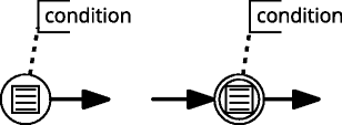
Conditional (start and intermediate) events
Full size image
Non-interruptive and Interruptive Boundary Conditional Events attached to a Task or a Subprocess can be used for interrupting a task or subprocess. The notation for conditional non-interruptive and interrputive boundary events are presented in Fig. 3.
Fig. 3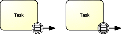
Conditional (non-interruptive and interrputive) boundary events
Full size image
Event Subprocess with Conditional Start Event can be used for interrupting the process and initiating a subprocess that is not a part of the regular control flow starting from the conditional start event. The notation for conditional non-interruptive and interrputive boundary events are presented in Fig. 4.
Fig. 4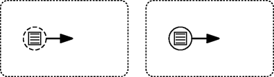
Event subprocesses with conditional start event
Full size image

Business Rule Task

Business Rule (BR) Tasks allow for specification of the task logic using rules and delegating work to a Business Rules Engine in order to receive calculated or inferred data. The notation for BR task is presented in Fig. 5.

For the BPMN Business Rule tasks, the following formulas have to be fullfiled in $\mathcal {M}$:

All BPMN BR tasks in $\mathcal {P}$ have the decision component from the $\mathbb {K}$ rule base assigned, i.e.:
$$\forall_{\tau \in \mathcal{T}_{\mathit{Business} \mathit{Rule}}} \; \exists_{t \in \mathbb{T}} \; \mathit{map}(\tau) = t. $$
All the input attributes required by the Business Rules Engine for a rule set specified by the decision component should be available in the process model, i.e.:
$$\forall_{\begin{array}{lllllll} \tau\in\mathcal{T}_{\mathit{Business} \mathit{Rule}}\\ t\in\mathbb{T}~~~~~~~~~~~~~~~\\ map(\tau) = t~~~~~~~ \end{array}} \, \forall_{r \in t} \,\forall_{\lambda \in \mathit{cond}(r)} \; \lambda \in \mathit{dataInputs}(\tau). $$
All the output attributes from the result of inference on a specified rule set from the Business Rules Engine should be available as the output of BR task in the process, i.e.:
$$\forall_{\begin{array}{llllllll} \tau\in\mathcal{T}_{\mathit{Business} \mathit{Rule}}\\ t\in\mathbb{T}\\ map(\tau) = t \end{array}} \,\, \forall_{r \in t} \,\forall_{\lambda \in \mathit{infer}(r)} \; \lambda \in \mathit{dataOutputs}(\tau) $$

Diverging (Exclusive, Inclusive/Multi-choice and Complex) Gateways

Gateways provide mechanisms for diverging a branch into two or more branches, and passing token from the incoming branch to one or more outgoing branches according to the type of a gateway.

For further formulae, the following sets are defined:

$$\begin{array}{@{}rcl@{}} \mathcal{G}^{\mathit{cond}}_{\mathit{div}} &\,=\,& \{g \in \mathcal{G}_{\times}\!\cup\mathcal{G}_{\circ}\!\cup\mathcal{G}_{\ast} \colon \mathit{\!gatewayDirection}(g) \,=\, \mathit{diverging}\},\\ \mathcal{F}_{g,\mathit{div}}^{\mathit{out},\mathit{cond}} &\,=\,& \{f \in \mathcal{F}_{g}^{\mathit{out}}\colon \!g \in \mathcal{G}^{\mathit{cond}}_{\mathit{div}} \wedge \mathit{default}(f) \!\neq\! \texttt{true}\},\\ \mathcal{F}_{g,\mathit{default}}^{\mathit{out},\mathit{cond}} &\,=\,& \{f \in \mathcal{F}_{g}^{\mathit{out}}\colon \!g \in \mathcal{G}^{\mathit{cond}}_{\mathit{div}} \wedge \mathit{default}(f) \,=\, \texttt{true}\}. \end{array} $$

In the case of exclusive ($\mathcal {G}_{\times }$), inclusive ($\mathcal {G}_{\circ }$) and complex ($\mathcal {G}_{\ast }$) diverging gateways (see Fig. 6), there is a need for the model $\mathcal {M}$ to satisfy the following requirements:

All BPMN sequence flows (apart from the default ones) outgoing from a diverging gateway have the condition in the form of a conditional part of a rule from the $\mathbb {K}$ rule base assigned, i.e.:
$$\begin{array}{@{}rcl@{}} && {}\forall_{f \in \mathcal{F}_{g,\mathit{div}}^{\mathit{out},\mathit{cond}}} \; \exists_{r \in \mathbb{R}} \; (map(f) = r) \wedge (\mathit{body}(f) = \mathit{cond}(r))\\ && {}\wedge (\mathit{language}(f) = \mathit{language}(r)). \end{array} $$
In the case of exclusive, inclusive and complex diverging gateways, they can have maximum one outgoing default sequence flow, i.e.:
$$\forall_{g \in \mathcal{G}^{\mathit{cond}}_{\mathit{div}}} ~~ |\mathcal{F}_{g,\mathit{default}}^{\mathit{out},\mathit{cond}}| \leq 1. $$
In the case of exclusive gateways, the evaluated conditions have to be exclusive, i.e.:
$$\begin{array}{@{}rcl@{}} && {}\forall_{f_{\mathit{1}},f_{\mathit{2}} \in \mathcal{F}_{g,\mathit{div}}^{\mathit{out}}} \; \forall_{g \in \mathcal{G}_{\times} } \; (~\exists_{r_{\mathit{1}},r_{\mathit{2}} \in \mathbb{R}} \; map(f_{\mathit{1}}) = r_{\mathit{1}} \wedge map(f_{\mathit{2}})\\ && {}= r_{\mathit{2}}) \Rightarrow (\mathit{eval}(r_{\mathit{1}}) \neq \mathit{eval}(r_{\mathit{2}})). \end{array} $$

Converging Complex Gateway

In the case of converging exclusive, inclusive and parallel gateways, their semantics is defined by the BPMN 2.0 specification and they do not require any rule-based description. However, a Converging Complex Gateway (see Fig. 7) requires an additional activationCondition expression which describes the precise behavior (defines the rule of passing tokens).

Thus, for BPMN Converging Complex Gateways the following requirements have to be fullfiled in $\mathcal {M}$:

All BPMN Converging Complex Gateways in $\mathcal {P}$ specify the rule of passing tokens, i.e.:
$$\begin{array}{@{}rcl@{}} && \forall_{g \in \mathcal{G}_{\ast}}\,\exists_{r \in \mathbb{R}}\;(\mathit{map}(g) = r) \wedge (\mathit{body}(g) = \mathit{cond}(r))\\ && \wedge (\mathit{language}(g) = \mathit{language}(r)), \end{array} $$
where activationCondition(g) = {body(g),language(g)}.
All condition attributes $\mathbb {A}_{r} \subset \mathbb {A}$ required by the rule r should be available in the process model, i.e.:
$$\forall_{r \in \mathbb{R}} \; \left( (\exists_{g \in \mathcal{G}_{\ast}} ~ \mathit{map}(g) = r)\Rightarrow (\forall_{\lambda \in \mathit{cond}(r)} \; \lambda \in {\Lambda}_{g}) \right). $$

Gateway Preceded by a BR Task

A special case of the two aboved examples occurs when a gateway is preceded by the BR task (Fig. 8). In the such case, there is a need for the model $\mathcal {M}$ to satisfy the requirements specified for Business Rule Tasks and for Gateways, as well as the following additional requirement:

All BPMN sequence flows (apart from the default sequence flows) outgoing from a diverging gateway preceded by the BR task have the conditions based on the output attributes of the BR task, i.e.:
$$\begin{array}{@{}rcl@{}} && \forall_{\begin{array}{llll} ~~~~~\tau\in\mathcal{T}_{\mathit{Business} \mathit{Rule}}\\ t\in\mathbb{T}~~~~~~~~~~~~~~~\\ ~~map(\tau) = t~~~~~~~ \end{array}} \, \forall_{g \in \mathcal{G}^{cond}_{div}} \; \left( (\tau,g,\lambda_{\tau g}) \in \mathcal{F} \right)\\ && \Rightarrow \left( \forall_{f \in \mathcal{F}_{g}^{\mathit{out}}} \forall_{\lambda \in \mathit{body}(f)} \; \lambda \in \mathit{infer}(t) \right). \end{array} $$
Fig. 8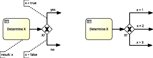
Gateway after BR task
Full size image

Gateway Preceded by a Subprocess

Another special case of using a gateway is a gateway preceded by a subprocess in which a decision is made (see Fig. 9). In such the case, there is a need for the model $\mathcal {M}$ to satisfy the requirements specified for Diverging Gateways, as well as the following additional requirements:

All BPMN sequence flows (apart from the default sequence flows) outgoing from a diverging gateway preceded by a subprocess have the conditions based on the attributes set by the preceded subprocess:
$$\begin{array}{@{}rcl@{}} && \forall_{s \in \mathcal{S}} \; \forall_{g \in \mathcal{G}^{cond}_{div}} \; \left( (s,g,\lambda_{s,g}) \in \mathcal{F} \right)\\ && \Rightarrow \left( \forall_{f \in \mathcal{F}_{g}^{\mathit{out}}}\; \forall_{\lambda \in \mathit{body}(f)}\; \lambda \in \mathit{dataOutputs}(s) \right). \end{array} $$
The number of sequence flows outgoing from a diverging gateway should be greater than or equal to the number of Message or None end events in the subprocess, i.e.:

Let: ${\mathcal {E}}_{End}^{s} = \{e \in \mathcal {O}_{s}\colon e \in {\mathcal {E}}_{End}^{None} \vee e \in {\mathcal {E}}_{End}^{Message}\}$, where $\mathcal {P}_{s} = (\mathcal {O}_{s}, \mathcal {F}_{s}, {\Lambda }_{s})$.

$\forall _{s \in \mathcal {S}} \; \forall _{g \in \mathcal {G}^{cond}_{div}} \; ((s,g,\lambda _{s,g}) \in \mathcal {F}) \Rightarrow (|\mathcal {F}_{g}^{out}| >= |\mathcal {E}^{s}_{End}| )$.

Event-Based Gateway

The use of Event-based (Exclusive) Gateway extends the use of Conditional Events (see Fig. 10). Thus, in this case, there is a need for the model $\mathcal {M}$ to satisfy the requirements specified for Conditional Events, as well as the following additional requirements:

All conditions in the Conditional Events that occur after the Event-based (Exclusive) Gateway should be exclusive,^{Footnote 12} i.e.:
$$\begin{array}{@{}rcl@{}} && \forall_{\begin{array}{lllllll} ~~~e_{\mathit{1}},e_{\mathit{1}} \in \mathcal{E}_{\mathit{Conditional}}\\ r_{\mathit{1}},r_{\mathit{1}} \in \mathbb{R} ~~~~~~~~~~~~~\\ \mathit{map}(e_{\mathit{1}}) = r_{\mathit{1}} ~~~~~~~~\\ \mathit{map}(e_{\mathit{2}}) = r_{\mathit{2}} ~~~~~~~~ \end{array}}\; \forall_{g \in \mathcal{G}_{\otimes}}\; ((g,e_{\mathit{1}},\lambda_{g,e_{\mathit{1}}}),\\ && \quad (g,e_{\mathit{2}},\lambda_{g,e_{\mathit{2}}})\in \mathcal{F})\\ && \Rightarrow \lnot \left( \mathit{eval}(r_{\mathit{1}}) \wedge \mathit{eval}(r_{\mathit{2}}) \right). \end{array} $$

Other BPMN Constructs

Although other BPMN elements or constructs are not directly associated with rules from the rule base, they can be described by rules. However, such a representation of rules is not formally defined in the model presented here.

In this section, a simple model of the integration of the BP model with rules was proposed. Moreover, this formal description provides the basis for refinement of the model for specific rule representation, e.g. the XTT2 representation from the SKE approach, which will be presented in the following sections.

5 SKE-Specific Business Logic Model

5.1 Semantic Knowledge Engineering Rules

Semantic Knowledge Engineering (SKE) (Nalepa 2011) is an approach that provides a coherent formal framework for eXtended Tabular Trees version 2 (XTT2) (Nalepa et al. 2011b), which is a rule-based knowledge representation language. The formalization of the XTT2 method based on the ALSV(FD) logic was presented by Nalepa and Ligęza in Nalepa (2010b, 2011). The goal of this section is to introduce the SKE-specific Business Logic Model, based on the General Business Logic Model presented in the previous section.

In order to formally define an XTT2 rule, the formal definitions for Attributive Logic with Set Values over Finite Domains (ALSV(FD)) are needed. ALSV(FD) is an extended version of Set Attributive Logic (SAL) (Ligęza 2006) oriented toward Finite Domains. It was discussed in (Nalepa 2010b). The expressive power of the ALSV(FD) formalism is increased through the introduction of new relational symbols. For simplicity, there are no objects specified in an explicit way. In ALSV(FD), A denotes the set of all attributes used to describe the system. Each attribute a_i ∈ A, i = 1…n has a set of admissible values that it takes (a domain) denoted as $\mathbb {D}_{i}$. Any domain is assumed to be a finite set.

Definition 9

An ALSV(FD)tripleε (also called a legal atomic formula in terms of the ALSV(FD) logic) is a triple of the form:

$$\varepsilon = (a_{i},\triangle,x_{i}) $$

where

a_i is an attribute,
x_i is the value of the attribute (it can be a single element of the domain or a subset of the domain),
△ is an operator from the set of operators for attributes,^{Footnote 13} such that △∈{=,≠,:=,∈,∉,⊆,⊇,∼,≁}.

The ALSV(FD) triples constitute the basic components of the XTT2 rules. A set consisting of the ALSV(FD) triples will be denoted by E, i.e. ε₁,ε₂,… ∈ E.

Definition 10

An XTT2 ruler_i (here called also rule) is a triple of the form:

$$r_{i} = (cond_{i}, dec_{i}) $$

where

cond_i ⊆ E is a conditional part of a rule consisting of legal atomic formulae in terms of ALSV(FD),
dec_i ⊆ E is a decision part of a rule consisting of legal atomic formulae in terms of ALSV(FD).

The set of all rules will be denoted as R, and r₁,r₂,… ∈ R. A rule schema for a given rule r_i (called also rule template) is a pair $schema(r_{i}) = (A^{cond}_{i}, A^{dec}_{i})$, where $A^{cond}_{i}$ and $A^{dec}_{i}$ are sets of all the attributes occurring in the conditional and decision part of the rule respectively.

From a logical point of view, the order of the ALSV(FD) atomic formulae in both the conditional and decision parts of the rule is unimportant. Having the structure of a single rule defined, the structure of the XTT2 rule base can be defined. The rule base is composed of tables grouping rules having the same lists of attributes (rule schemas). Rule schemas are used to identify rules working in the same situation (operational context). Such a set of rules can form a decision component in the form of a decision table. A common schema can also be considered as a table header.

Definition 11

An XTT2 decision componentt (also called an XTT2 table) is a sequence of rules having the same rule schema:

$$t = (r_{1}, r_{2}, {\ldots} ,r_{n}) $$

The set of decision components is denoted as T, t₁,t₂,... ∈ T. An XTT2 table schema (also called a schema of the component or table header) is denoted as schema(t).

5.2 Integrated Model

The SKE-specific Business Logic Model is a special case of the General Business Logic Model that describes the integration of the BPMN process models with the SKE rules.

Definition 12

SKE-specific Business Logic Model is a tuple: $\mathcal {M}_{SKE} = (\mathcal {P}, \mathbb {K}_{SKE}, \mathit {map})$, where:

$\mathbb {K}_{SKE} = (\mathbb {A}_{SKE}, \mathbb {R}_{SKE}, \mathbb {T}_{SKE}) = (A, R, T_{\mathcal {X}})$ is an SKE-specific rule base, where:
- $T_{\mathcal {X}}$ is a set of the XTT2 decision components,
- R is a set of the XTT2 rules, such as:
  $$R = \{r_{i} \in t\colon t \in T_{\mathcal{X}}\}, $$
  $$\forall_{r_{i} \in R} \; schema(r_{i}) = schema(t), $$
  and the conditional cond(r_i) part of a rule is defined as follows:
  $$\mathit{cond}(r_{i}) = E^{cond}_{i}, $$
  where $r_{i} = (E^{cond}_{i}, E^{dec}_{i}, ACT_{i})$,
- A is a set of the attributes used in the XTT2 rule base, i.e.:^{Footnote 14}
  $$A = \{a_{i}\colon \exists_{r_{i} \in R} \; a_{i} \in A^{cond}_{i} \vee a_{i} \in A^{dec}_{i} \}. $$
$\mathcal {P}$ is a BPMN 2.0 process model,
map is a mapping function between the elements of the $\mathcal {P}$ process model and the elements of the $\mathbb {K}_{SKE}$ rule base.

The $\mathbb {K}_{SKE}$ rule base specifies the value of language, such as: $\forall _{r_{i} \in R} \; \mathit {language}(r) =$ “XTT2”. Moreover, the infer(t) method is defined as follows: $\mathit {infer}(t) = A^{dec}_{t}$. This stems from the fact that in the SKE-specific Business Logic Model, every decision component $t \in T_{\mathcal {X}}$ is an XTT2 decision table. Thus, the result of the inference is the set of decision attributes of this decision table.^{Footnote 15}

In the following paragraphs, the integration details are specified.^{Footnote 16}

References

Bădică, A., & Bădică, C. (2011). Formal verification of business processes as role activity diagrams. In 2011 Federated Conference on computer science and information systems (FedCSIS) (pp. 277–280): IEEE.
Bădică, C., Bădică, A., Litoiu, V. (2003). Role activity diagrams as finite state processes. In Proceedings of the second international conference on parallel and distributed computing ISPDC’03, Ljubljana, Slovenia, October 13–14, 2003 (pp. 15–22).
Batoulis, K., Baumgrass, A., Herzberg, N., Weske, M. (2015a). Enabling dynamic decision making in business processes with DMN. In International conference on business process management (pp. 418–431): Springer.
Batoulis, K., Meyer, A., Bazhenova, E., Decker, G., Weske, M. (2015b). Extracting decision logic from process models. In International conference on advanced information systems engineering (pp. 349–366): Springer.
Bazhenova, E., & Weske, M. (2015). Deriving decision models from process models by enhanced decision mining. In International conference on business process management (pp. 444–457): Springer.
Catalkaya, S., Knuplesch, D., Chiao, C., Reichert, M. (2013). Enriching business process models with decision rules. In International conference on business process management (pp. 198–211): Springer.
Changizi, B., Kokash, N., Arbab, F. (2010). A unified toolset for business process model formalization. In Proceeding of the 7th international workshop on formal engineering approaches to software components and architectures, satellite event of ETAPS, held on 27th March 2010, Paphos, Cyprus (p. 10).
Charfi, A., & Mezini, M. (2004). Hybrid web service composition: business processes meet business rules. In Proceedings of the 2nd international conference on service-oriented computing, ICSOC ’04 (pp. 30–38). New York: ACM.
Debevoise, T., Taylor, J., Sinur, J., Geneva, R. (2014). The MicroGuide to process and decision modeling in BPMN/DMN: building more effective processes by integrating process modeling with decision modeling. CreateSpace Independent Publishing Platform.
Dijkman, R.M., & Gorp, P.V. (2011). Bpmn 2.0 execution semantics formalized as graph rewrite rules. In Mendling, J., Weidlich, M., Weske, M. (Eds.) Proceedings from the business process modeling notation—second international workshop, BPMN 2010, Potsdam, Germany, October 13–14, 2010. Lecture notes in business information processing, (Vol. 67 pp. 16–30): Springer.
Dijkman, R.M., Dumas, M., Ouyang, C. (2007). Formal semantics and automated analysis of BPMN process models. preprint 7115. Tech. rep. Queensland University of Technology, Brisbane, Australia.
Dumas, M., La Rosa, M., Mendling, J., Reijers, H.A. (2013). Fundamentals of business process management. Berlin: Springer.
Hohwiller, J., Schlegel, D., Grieser, G., Hoekstra, Y. (2011). Integration of BPM and BRM. In Dijkman, R., Hofstetter, J., Koehler, J. (Eds.) Business process model and notation, Lecture notes in business information processing, (Vol. 95 pp. 136–141). Berlin: Springer. https://doi.org/10.1007/978-3-642-25160-3_12.
Janssens, L., Bazhenova, E., De Smedt, J., Vanthienen, J., Denecker, M. (2016). Consistent integration of decision (DMN) and process (BPMN) models. In Proceedings of the CAiSE’16 forum, at the 28th international conference on advanced information systems engineering (CAiSE 2016), Ljubljana, Slovenia, June 13–17, 2016 (pp. 121–128).
Kaczor, K. (2015). Practical approach to interoperability in production rule bases with SUBITO. In Rutkowski, L. et al. (Eds.) Artificial intelligence and soft computing: 14th international conference, ICAISC 2015, Lecture notes in artificial intelligence. Accepted. Zakopane: Springer.
Kluza, K. (2015). Methods for modeling and integration of business processes with rules. PhD thesis, AGH University of Science and Technology, Supervisor: Grzegorz J. Nalepa.
Kluza, K., & Nalepa, G.J. (2017). A method for generation and design of business processes with business rules. Information and Software Technology, 91, 123–141.
Kluza, K., Kaczor, K., Nalepa, G.J. (2012). Enriching business processes with rules using the Oryx BPMN editor. In Rutkowski, L. et al. (Eds.) Artificial intelligence and soft computing: 11th international conference, ICAISC 2012: Zakopane, Poland, April 29–May 3, 2012, Lecture notes in artificial intelligence, (Vol. 7268 pp. 573–581): Springer. http://www.springerlink.com/content/u654r0m56882np77/.
Kluza, K., Kaczor, K., Nalepa, G.J. (2015). Integration of business processes with visual decision modeling. Presentation of the hades toolchain. In Fournier, F., & Mendling, J. (Eds.) Business process management workshops. BPM 2014 international workshops, Eindhoven, The Netherlands, September 7–8, 2014, Revised Papers, Lecture notes in business information processing, (Vol. 202 pp. 504–515): Springer International Publishing. https://doi.org/10.1007/978-3-319-15895-2_43.
Knolmayer, G., Endl, R., Pfahrer, M. (2000). Modeling processes and workflows by business rules. In Business process management, models, techniques, and empirical studies (pp. 16–29). London: Springer.
Lam, V.S.W. (2009). Equivalences of BPMN processes. Service Oriented Computing and Applications, 3(3), 189–204.
Lam, V.S.W. (2012). Foundation for equivalences of BPMN models. Theoretical and Applied Informatics, 24 (1), 33–66.
Ligęza, A. (1999). Intelligent data and knowledge analysis and verification; towards a taxonomy of specific problems. In Vermesan, A., & Coenen, F. (Eds.) Validation and verification of knowledge based systems (pp. 313–325): Springer. https://doi.org/10.1007/978-1-4757-6916-6_21.
Ligęza, A. (2006). Logical foundations for rule-based systems. Berlin: Springer.
Ligęza, A. (2011). BPMN – a logical model and property analysis. Decision Making in Manufacturing and Services, 5(1-2), 57–67.
Lindsay, A., Dawns, D., Lunn, K. (2003). Business processes – attempts to find a definition. Information and Software Technology, 45(15), 1015–1019.
Nalepa, G.J. (2010a). Architecture of the HeaRT hybrid rule engine. In Rutkowski, L. et al. (Eds.) Artificial intelligence and soft computing: 10th international conference, ICAISC 2010: Zakopane, Poland, June 13–17, 2010, Pt. II, Lecture notes in artificial intelligence, (Vol. 6114 pp. 598–605): Springer.
Nalepa, G.J. (2010b). HeKatE methodology, hybrid engineering of intelligent systems. International Journal of Applied Mathematics and Computer Science, 20(1), 35–53.
Nalepa, G.J. (2011). Semantic knowledge engineering a rule-based approach. Kraków: Wydawnictwa AGH.
Nalepa, G.J., & Ligęza, A. (2005). Software engineering: evolution and emerging technologies, frontiers in artificial intelligence and applications. In Conceptual modelling and automated implementation of rule-based systems, (Vol. 130 pp. 330–340). Amsterdam: IOS Press.
Nalepa, G., Bobek, S., Ligęza, A., Kaczor, K. (2011a). HalVA – rule analysis framework for XTT2 rules. In Bassiliades, N., Governatori, G., Paschke, A. (Eds.) Rule-based reasoning, programming, and applications, Lecture notes in computer science, (Vol. 6826 pp. 337–344). Berlin: Springer. http://www.springerlink.com/content/c276374nh9682jm6/.
Nalepa, G., Ligęza, A., Kaczor, K. (2011b). Overview of knowledge formalization with XTT2 rules. In Bassiliades, N., Governatori, G., Paschke, A. (Eds.) Rule-based reasoning, and programming, and applications, Lecture notes in computer science, (Vol. 6826 pp. 329–336). Berlin: Springer.
Nalepa, G.J., Ligęza, A., Kaczor, K. (2011c). Formalization and modeling of rules using the XTT2 method. International Journal on Artificial Intelligence Tools, 20(6), 1107–1125.
Nalepa, G.J., Kluza, K., Kaczor, K. (2013). Proposal of an inference engine architecture for business rules and processes. In Rutkowski, L. et al. (Eds.) Artificial intelligence and soft computing: 12th international conference, ICAISC 2013: Zakopane, Poland, June 9–13, 2013, Lecture notes in artificial intelligence, (Vol. 7895 pp. 453–464): Springer. http://www.springer.com/computer/ai/book/978-3-642-38609-1.
OMG. (2006). Semantics of business vocabulary and business rules (SBVR). Tech. Rep. dtc/06-03-02, Object Management Group.
OMG. (2011a). Business process model and notation (BPMN): Version 2.0 specification. Tech. Rep. formal/2011-01-03, Object Management Group.
OMG. (2011b). Decision model and notation request for proposal. Tech. Rep. bmi/2011-03-04, Object Management Group, 140 Kendrick Street, Building A Suite 300, Needham, MA 02494, USA.
OMG. (2015). Decision model and notation (DMN). Version 1.0: Formal Specification. Tech. rep., Object Management Group (OMG). http://www.omg.org/spec/DMN/1.0/Beta2/.
Ouyang, C., Wil, M.P., van der Aalst, M.D., ter Hofstede, A.H. (2006a). Translating BPMN to BPEL. Tech. rep., Faculty of Information Technology, Queensland University of Technology, GPO Box 2434, Brisbane QLD 4001, Australia Department of Technology Management, Eindhoven University of Technolog y, GPO Box 513, NL-5600 MB, The Netherlands.
Ouyang, C., Dumas, M., ter Hofstede, A.H., van der Aalst, W.M. (2006b). From BPMN process models to BPEL web services. In IEEE international conference on web service (ICWS’06).
Sivaraman, E., & Kamath, M. (2002). On the use of Petri nets for business process modeling. In Proceeding of the 11th annual industrial engineering research conference.
Smirnov, S., Weidlich, M., Mendling, J., Weske, M. (2012). Action patterns in business process model repositories. Computers in Industry, 63(2), 98–111.
Speck, A., Feja, S., Witt, S., Pulvermüller, E., Schulz, M. (2011). Formalizing business process specifications. Computer Science and Information Systems/ComSIS, 8(2), 427–446.
Szpyrka, M., Nalepa, G.J., Ligęza, A, Kluza, K. (2011). Proposal of formal verification of selected BPMN models with Alvis modeling language. In Brazier, F.M., Nieuwenhuis, K., Pavlin, G., Warnier, M., Badica, C. (Eds.) Intelligent distributed computing V. Proceedings of the 5th international symposium on intelligent distributed computing – IDC 2011, Delft, the Netherlands – October 2011, Studies in computational intelligence, (Vol. 382 pp. 249–255): Springer. http://www.springerlink.com/content/m181144037q67271/.
van der Aa, H., Leopold, H., Batoulis, K., Weske, M., Reijers, H.A. (2016). Integrated process and decision modeling for data-driven processes. In Business process management workshops. BPM 2015 international workshops, Innsbruck, Austria, August 31–September 3, 2015, Revised Papers, Lecture notes in business information processing (pp. 405–417): Springer International Publishing. https://doi.org/10.1007/978-3-319-42887-1_33.
Wagner, G., Giurca, A., Lukichev, S. (2005). R2ML: a general approach for marking up rules. In Bry, F., Fages, F., Marchiori, M., Ohlbach, H. (Eds.) Principles and practices of semantic web reasoning, Dagstuhl seminar proceedings (p. 05371).
Wang, W., Indulska, M., Sadiq, S., Weber, B. (2017). Effect of linked rules on business process model understanding. In International conference on business process management, (Vol. 10445, pp. 200–215). Springer.
Weske, M. (2012). Business process management: concepts, languages, architectures, 2nd edn. Berlin: Springer.
Wong, P.Y.H., & Gibbons, J. (2008). A process semantics for BPMN. In Liu, S., Maibaum, T.S.E., Araki, K. (Eds.) Proceedings from the 10th international conference on formal engineering methods, ICFEM 2008, Kitakyushu-City, Japan, October 27–31, 2008, Lecture notes in computer science, (Vol. 5256 pp. 355–374): Springer.
Wong, P.Y.H., & Gibbons, J. (2011). Formalisations and applications of BPMN. Science of Computer Programming, 76(8), 633–650.
Wynn, M., Verbeek, H., Wvd, A., At, H., Edmond, D. (2009). Business process verification – finally a reality!. Business Process Management Journal, 1(15), 74–92.
Acknowledgements
The research presented in this paper is partially based on the PhD thesis (Kluza 2015) of the first author and is supported by the HiBuProBuRul Project funded from NCN (National Science Centre) resources for science (no. DEC-2011/03/N/ST6/00909).
Author information
Authors and Affiliations
Corresponding author
Additional information
The research presented in this paper is supported by the HiBuProBuRul Project funded from NCN (National Science Centre) resources for science (no. DEC-2011/03/N/ST6/00909).
Rights and permissions
Open Access This article is distributed under the terms of the Creative Commons Attribution 4.0 International License (http://creativecommons.org/licenses/by/4.0/), which permits unrestricted use, distribution, and reproduction in any medium, provided you give appropriate credit to the original author(s) and the source, provide a link to the Creative Commons license, and indicate if changes were made.
About this article