Interrupt Timed Automata: verification and expressiveness

Abstract

We introduce the class of Interrupt Timed Automata (ITA), a subclass of hybrid automata well suited to the description of timed multi-task systems with interruptions in a single processor environment.

While the reachability problem is undecidable for hybrid automata we show that it is decidable for ITA. More precisely we prove that the untimed language of an ITA is regular, by building a finite automaton as a generalized class graph. We then establish that the reachability problem for ITA is in NEXPTIME and in PTIME when the number of clocks is fixed. To prove the first result, we define a subclass ITA₋ of ITA, and show that (1) any ITA can be reduced to a language-equivalent automaton in ITA₋ and (2) the reachability problem in this subclass is in NEXPTIME (without any class graph).

In the next step, we investigate the verification of real time properties over ITA. We prove that model checking SCL, a fragment of a timed linear time logic, is undecidable. On the other hand, we give model checking procedures for two fragments of timed branching time logic.

We also compare the expressive power of classical timed automata and ITA and prove that the corresponding families of accepted languages are incomparable. The result also holds for languages accepted by controlled real-time automata (CRTA), that extend timed automata. We finally combine ITA with CRTA, in a model which encompasses both classes and show that the reachability problem is still decidable. Additionally we show that the languages of ITA are neither closed under complementation nor under intersection.

Appendices

Appendix A: Proof of Theorem 4

Let φ be a formula in $\mathsf{TCTL}_{c}^{\mathrm{int}}$ and $\mathcal{A}$ an ITA with n levels and E transitions. Like in Sect. 3, the proof relies on the construction of a finite class graph. The main difference is in the computation of the n sets of expressions E ₁,…,E _n . Like before, each set E _k is initialized to {x _k ,0} and expressions in this set are those which are relevant for comparisons with the current clock at level k. In this case, they include not only guards but also comparisons with the constraints from the formula. Recall that the sets are computed top down from n to 1, using the normalization operation.

• At level k, we may assume that expressions in guards of an edge leaving a state are of the form αx _k +∑ _i<k a _i x _i +b with α∈{0,1}. We add −∑ _i<k a _i x _i −b to E _k .

• To take into account the constraints of formula φ, we add the following step: For each comparison C⋈0 in φ, and for each k, with norm(C,k)=αx _k +∑ _i<k a _i x _i +b (α∈{0,1}), we also add expression −∑ _i<k a _i x _i −b to E _k .

• Then we iterate the following procedure until no new term is added to any E _i for 1≤i≤k.

  • 1. Let $q \xrightarrow{\varphi,a,u} q'$ with λ(q′)≥k and λ(q)≥k. If C∈E _k , then we add C[u] to E _k .

  • 2. Let $q \xrightarrow{\varphi,a,u} q'$ with λ(q′)≥k and λ(q)<k. For C,C′∈E _k , we compute C″=norm(C[u]−C′[u],λ(q)). If C″=αx _λ(q)+∑ _i<λ(q) a _i x _i +b with α∈{0,1}, then we add −∑ _i<λ(q) a _i x _i −b to E _λ(q).

The proof of termination for this construction is similar to the one in Sect. 3.

We now consider the transition system $\mathcal{G}_{\mathcal{A}}$ whose set of configurations are the classes R=(q,{⪯ _k }_{1≤k≤λ(q)}), where q is a state and ⪯ _k is a total preorder over E _k . The class R describes the set of valuations 〚R〛={(q,v)∣∀k≤λ(q) ∀(g,h)∈E _k , g[v]≤h[v] iff g⪯ _k h}. The set of transitions is defined as in Sect. 3. The transition system $\mathcal{G}_{\mathcal{A}}$ is again finite and time abstract bisimilar to $\mathcal{T}_{\mathcal{A}}$. Moreover, the truth value of each comparison C=∑ _i≥1 a _i ⋅x _i +b⋈0 appearing in φ can be set for each class R. Indeed, since for every k, both 0 and $\sum_{i \geq1}^{k-1}a_{i} \cdot x_{i} + b$ are in the set of expressions E _k , the truth value of C⋈0 does not change inside a class. Therefore, introducing a fresh propositional variable q _C for the constraint C⋈0, each class R can be labelled with a truth value for each q _C . Deciding the truth value of φ can then be done by a classical CTL model-checking algorithm on $\mathcal {G}_{\mathcal{A}}$.

The complexity of the procedure is obtained by bounding the number of expressions for each level k by $(E+|\varphi|+2)^{2^{n(n-k+1)}+1}$, and applying the same reasoning as for Proposition 2.

Appendix B: Proof of Theorem 7

We build an automaton in ITA×TA which simulates a deterministic two counter machine $\mathcal{M}$ (as in proof of Theorem 3).

Let $L_{\mathcal{M}}$ be the set of labels of $\mathcal{M}$. The automaton $\mathcal{A}_{\mathcal{M}} =\langle \varSigma ,Q,q_{0},F,\mathit{pol},X \cup Y,\lambda,\varDelta \rangle$ is built to reach its final location Halt if and only if $\mathcal{M}$ stops. It is defined as follows:

• Σ consists of one letter per transition.

• $Q = L_{\mathcal{M}}\cup(L _{\mathcal{M}}\times\{k_{0}\}) \cup (L_{\mathcal{M}}\times \{k_{1},k_{2},r_{1},\ldots,r_{5}\} \times\{>,<\})$, q ₀=ℓ ₀ (the initial instruction of $\mathcal{M}$) and F={Halt}.

• pol:Q→{Urgent,Lazy,Delayed} is such that pol(q)=Urgent iff either $q \in L_{\mathcal{M}}$ or q=(ℓ,q ₂,⋈), and pol(q)=Lazy in most other cases: some states (ℓ,k _i ,⋈) are Delayed, as shown on Figs. 21 and 22.

  Fig. 21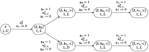

  

  Module taking into account the order between the values of c and d when incrementing c

  Fig. 22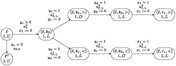

  

  Module taking into account the order between the values of c and d when decrementing c

• X={x ₁,x ₂,x ₃} is the set of interrupt clocks and Y={y _c ,y _d } is the set of standard clocks with rate 1.

• λ:Q→{1,2,3} is the interrupt level of each state. All states in $L_{\mathcal{M}}$ and $L_{\mathcal{M}}\times\{k_{0},k_{1},k_{2}\}$ are at level 1; so do all states corresponding to r ₁. States corresponding to r ₂ and r ₃ are in level 2, while the ones corresponding to r ₄ and r ₅ are in level 3.

• Δ is defined through basic modules in the sequel.

The transitions of $\mathcal{A}_{\mathcal{M}}$ are built within small modules, each one corresponding to one instruction of $\mathcal{M}$. The value n of c (resp. p of d) in a state of $L_{\mathcal{M}}$ is encoded by the value $1 - \frac{1}{2^{n}}$ of clock y _c (resp. $1 -\frac{1}{2^{p}}$ of y _d ).

The idea behind this construction is that for any standard clock y, it is possible to “copy” the value of k−y in an interrupt clock x _i , for some constant k, provided the value of y never exceeds k. To achieve this, we start and reset the interrupt clock, then stop it when y=k. Note that by the end of the copy, the value of y has changed. Conversely, in order to copy the content of an interrupt clock x _i into a clock y, we switch from level i to level i+1 and reset y at the same time. When x _i+1=x _i , the value of y is equal to the value of x _i . Remark that the form of the guards on x _i+1 allows us to copy the value of a linear expression on {x ₁,…,x _i } in y.

For instance, consider an instruction labeled by ℓ incrementing c then going to ℓ′, with the respective values n of c and p of d, from a configuration where n≥p. The corresponding module $\mathcal{A}_{c\geq d}^{c++}(\ell,\ell')$ is depicted on Fig. 18 (see main text). In this module, interrupt clock x ₁ is used to record the value $\frac{1}{2^{n}}$ while x ₂ keeps the value $\frac{1}{2^{p}}$. Assuming that $y_{c} = 1 - \frac{1}{2^{n}}$, $y_{d} = 1 - \frac{1}{2^{p}}$ and x ₁=0 in state (ℓ,r ₁,>), the unique run in $\mathcal{A}_{c\geq d}^{c++}(\ell,\ell')$ will end in state ℓ′ with $y_{c} = 1 - \frac{1}{2^{n+1}}$ and $y_{d} = 1 -\frac{1}{2^{p}}$. The intermediate clock values are shown in Table 3 (see main text).

The module on Fig. 18 can be adapted for the case of decrementing c by just changing the linear expressions in guards for x ₃, provided that the final value of c is still greater than the one of d. It is however also quite easy to adapt the same module when n<p: in that case we store $\frac{1}{2^{p}}$ in x ₁ and $\frac{1}{2^{n}}$ in x ₂, since y _d will reach 1 before y _c . We also need to start y _d before y _c when copying the adequate values in the clocks. The case of decrementing c while n≤p is handled similarly. In order to choose which module to use according to the ordering between the values of the counters, we use the modules of Figs. 21 and 22. Figure 21 represents the case when at label ℓ we have an increment of c whereas Fig. 22 represents the case when ℓ corresponds to decrementing c. In that last case the value of c is compared not only to the one of d, but also to 0, in order to know which branch of the if instruction is taken. Note that only one of the branches can be taken until the end.⁶ Instructions involving d are handled in a symmetrical way.

Automaton $\mathcal{A}_{\mathcal{M}}$ is obtained by joining the modules described above through the states of $L_{\mathcal{M}}$. Let us prove that automaton $\mathcal{A}_{\mathcal{M}}$ simulates the two counter machine $\mathcal{M}$, so that $\mathcal{M}$ halts iff $\mathcal{A}_{\mathcal{M}}$ reaches the Halt state.

Let 〈ℓ ₀,0,0〉〈ℓ ₁,n ₁,p ₁〉…〈ℓ _i ,n _i ,p _i 〉… be a run of $\mathcal{M}$. We show that this run is simulated in $\mathcal{A}_{\mathcal{M}}$ by the run 〈l ₀,0〉ρ ₀〈l ₁,v ₁〉ρ ₁… where ρ _i is either empty or a subrun through states in {(ℓ _i ,r _j ,⋈) | j∈{1,…,5},⋈ ∈{>,<}} (i.e. subruns in modules like $\mathcal{A}^{c++}_{c \geq d}$ of Fig. 18). Moreover, it will be the case that

$$\forall i,\quad v_i(y_c) = 1 -\frac{1}{2^{n_i}} \quad\mathrm{and} \quad v_i(y_d) = 1 -\frac{1}{2^{p_i}}$$

This holds at the beginning of the execution of $\mathcal{A}_{\mathcal{M}}$. Suppose that we have simulated the subrun up to 〈ℓ _i ,n _i ,p _i 〉. Then we are in state ℓ _i , with clock y _c being $1 - \frac{1}{2^{n_{i}}}$ and y _d being $1 - \frac{1}{2^{p_{i}}}$. The next configuration of $\mathcal{M}$, 〈ℓ _i+1,n _i+1,p _i+1〉, depends on the content of instruction ℓ _i , and so does the outgoing transitions of state ℓ _i in $\mathcal{A}_{\mathcal{M}}$. We consider the case where ℓ _i decrements c and goes to ℓ′ if c is greater than 0 and goes to ℓ″ otherwise, the other ones being similar. We are therefore in the case of Fig. 22. If n _i =0, the next configuration of $\mathcal{M}$ will be 〈ℓ″,n _i ,p _i 〉. Conversely, in $\mathcal{A}_{\mathcal{M}}$, if n _i =0 then y _c =0, and there is no choice but to enter ℓ″, leaving all clock values unchanged (because ℓ _i is an Urgent state). The configuration of $\mathcal{A}_{\mathcal{M}}$ thus satisfies the property. If n _i >0, the next configuration of $\mathcal{M}$ will be 〈ℓ′,n _i −1,p _i 〉. In $\mathcal{A}_{\mathcal{M}}$, the transition chosen is the one that corresponds to the ordering between n _i and p _i . In both cases, similarly to the example of $\mathcal{A}^{c++}_{c \geq d}(\ell,\ell')$, the run reaches state ℓ′ with $y_{c} =1 -\frac{1}{2^{n_{i}-1}}$ and y _d as before, thus preserving the property. Hence $\mathcal{M}$ halts iff $\mathcal{A}_{\mathcal{M}}$ reaches the Halt state.

The automaton $\mathcal{A}_{\mathcal{M}}$ is indeed the product of an ITA $\mathcal{I}$ and a TA $\mathcal{T}$, synchronized on actions. Observe that in all the modules described above, guards never mix a standard clock with an interrupt one. Since each transition has a unique label, keeping only guards and resets on either the clocks of X or on those of Y yields an ITA and a TA whose product is $\mathcal{A}_{\mathcal{M}}$.

References

Aceto L, Burgueño A, Larsen KG (1998) Model checking via reachability testing for timed automata. In: Proceedings of the 4th international conference on tools and algorithms for construction and analysis of systems (TACAS’98). Lecture notes in computer science, vol 1384. Springer, London, pp 263–280
Alur R, Dill DL (1994) A theory of timed automata. Theor Comput Sci 126:183–235
Alur R, Courcoubetis C, Dill DL (1993) Model-checking in dense real-time. Inf Comput 104:2–34
Alur R, Courcoubetis C, Halbwachs N, Henzinger TA, Ho PH, Nicollin X, Olivero A, Sifakis J, Yovine S (1995) The algorithmic analysis of hybrid systems. Theor Comput Sci 138:3–34
Alur R, Feder T, Henzinger TA (1996) The benefits of relaxing punctuality. J ACM 43(1):116–146
Asarin E, Maler O, Pnueli A (1995) Reachability analysis of dynamical systems having piecewise-constant derivatives. Theor Comput Sci 138(1):35–65
Asarin E, Schneider G, Yovine S (2007) Algorithmic analysis of polygonal hybrid systems, part I: Reachability. Theor Comput Sci 379(1–2):231–265
Behrmann G, David A, Larsen KG (2004) A tutorial on uppaal. In: Formal methods for the design of real-time systems (SFM-RT’04). Lecture notes in computer science, vol 3185. Springer, Berlin, pp 200–236
Bérard B, Haddad S (2009) Interrupt timed automata. In: Proceedings of the 12th international conference on foundations of software science and computation structures (FoSSaCS’09). Lecture notes in computer science, vol 5504. York, GB. Springer, Berlin (March 2009), pp 197–211
Bérard B, Petit A, Diekert V, Gastin P (1998) Characterization of the expressive power of silent transitions in timed automata. Fundam Inform 36(2–3):145–182
Bérard B, Haddad S, Sassolas M (2010) Real time properties for interrupt timed automata. In: Markey N, Wisjen J (eds) Proceedings of the 17th international symposium on temporal representation and reasoning (TIME’10). IEEE Computer Society, Washington (September 2010), pp 69–76
Bouyer P (2004) Forward analysis of updatable timed automata. Form Methods Syst Des 24(3):281–320
Bouyer P, Chevalier F, Markey N (2005) On the expressiveness of TPTL and MTL. In: Proceedings of the 25th conference on foundations of software technology and theoretical computer science (FSTTCS’05). Lecture notes in computer science, vol 3821. Springer, Berlin (December 2005), pp 432–443
Bouyer P, Brihaye Th, Jurdziński M, Lazić R, Rutkowski M (2008) Average-price and reachability-price games on hybrid automata with strong resets. In: Cassez F, Jard C (eds) Proceedings of the 6th international conference on formal modelling and analysis of timed systems (FORMATS’08), Saint-Malo, France. Lecture notes in computer science, vol 5215. Springer, Berlin (September 2008), pp 63–77
Bozga M, Daws C, Maler O, Olivero A, Tripakis S, Yovine S (1998) KRONOS: A model-checking tool for real-time systems. In: FTRTFT, pp 298–302
Brihaye T, Bruyère V, Raskin JF (2006) On model-checking timed automata with stopwatch observers. Inf Comput 204(3):408–433
Brihaye T, Doyen L, Geeraerts G, Ouaknine J, Raskin JF, Worrell J (2010) On reachability for hybrid automata over bounded time. In: Aceto L, Henzinger M, Sgall J (eds) Proceedings (part II) of the 38th international colloquium on automata, languages and programming (ICALP’11). Lecture notes in computer science, vol 6756. Springer, Berlin (July 2011), pp 416–427
Cassez F, Larsen KG (2000) The impressive power of stopwatches. In: Palamidessi C (ed) Proceedings of the 11th international conference on concurrency theory (CONCUR’00). Lecture notes in computer science, vol 1877. Springer, Berlin, pp 138–152
Cimatti A, Clarke E, Giunchiglia E, Giunchiglia F, Pistore M, Roveri M, Sebastiani R, Tacchella A (2002) NuSMV version 2: An opensource tool for symbolic model checking. In: Proceedings of the 14th international conference on computer aided verification (CAV’02). Lecture notes in computer science, vol 2404. Springer, Berlin, pp 241–268
Courcoubetis C, Yannakakis M (1992) Minimum and maximum delay problems in real-time systems. Form Methods Syst Des 1(4):385–415
Demichelis F, Zielonka W (1998) Controlled timed automata. In: Sangiorgi D, de Simone R (eds) Proceedings of the 9th international conference on concurrency theory (CONCUR’98). Lecture notes in computer science, vol 1466. Springer, London, pp 455–469
Emerson EA, Halpern JY (1982) Decision procedures and expressiveness in the temporal logic of branching time. In: Proc 14th annual ACM symp on theory of computing (Stoc’82). ACM, New York, pp 169–180
Fersman E, Krcal P, Pettersson P, Yi W (2007) Task automata: Schedulability, decidability and undecidability. Inf Comput 205(8):1149–1172
Henzinger TA, Nicollin X, Sifakis J, Yovine S (1994) Symbolic model checking for real-time systems. Inf Comput 111(2):193–244
Henzinger TA, Kopke PW, Puri A, Varaiya P (1998) What’s decidable about hybrid automata? J Comput Syst Sci 57(1):94–124
Kesten Y, Pnueli A, Sifakis J, Yovine S (1999) Decidable integration graphs. Inf Comput 150(2):209–243
Koymans R (1990) Specifying real-time properties with metric temporal logic. Real-Time Syst 2:255–299
Lafferriere G, Pappas GJ, Yovine S (1999) A new class of decidable hybrid systems. In: Proceedings of hybrid systems: Computation and control. Lecture notes in computer science, vol 1569. Springer, Berlin, pp 137–151
Lafferriere G, Pappas GJ, Yovine S (2001) Symbolic reachability computation for families of linear vector fields. J Symb Comput 32(3):231–253
Maler O, Manna Z, Pnueli A (1992) From timed to hybrid systems. In: Rozenberg G, de Roever WP, Huizing C, de Bakker JW (eds) Real-time: theory in practice, REX workshop. Lecture notes in computer science, vol 600. Springer, Berlin, pp 447–484
McManis J, Varaiya P (1994) Suspension automata: A decidable class of hybrid automata. In: Proceedings of the 6th international conference on computer aided verification (CAV’94). Springer, London, pp 105–117
Minsky ML (1967) Computation: Finite and infinite machines. Prentice-Hall, Inc, Upper Saddle River
Pnueli A (1977) The temporal logic of programs. In: Proceedings of the 18th annual symposium on foundations of computer science (FoCS’77). IEEE Computer Society, Washington, pp 46–57
Queille JP, Sifakis J (1982) Specification and verification of concurrent systems in CESAR. In: Dezani-Ciancaglini M, Montanari U (eds) Proceedings of the 5th international symposium on programming. Lecture notes in computer science, vol 137. Springer, London, pp 337–351
Raskin JF, Schobbens PY (1997) State clock logic: A decidable real-time logic. In: Maler O (ed) Hybrid and real-time systems. Lecture notes in computer science, vol 1201. Springer, Berlin, pp 33–47
Roos C, Terlaky T, Vial JP (1997) Theory and algorithms for linear optimization. An interior point approach. Wiley-Interscience, New York
Silberschatz A, Galvin PB, Gagne G (2008) Operating systems concepts, 8th edn. Wiley, New York
Sistla AP, Clarke EMM (1985) The complexity of propositional linear temporal logics. J ACM 32:733–749
Zaslavsky T (1975) Facing up to arrangements: Face-count formulas for partitions of space by hyperplanes. AMS Mem 1(154)
Acknowledgements
The authors would like to thank the anonymous reviewers for their insightful comments. This work was supported by projects Dots (ANR-06-SETI-003, French government), ImpRo (ANR-2010-BLAN-0317, French government) and CoChaT (Digiteo 2009-27HD, Région Île de France).
Author information
Authors and Affiliations
Corresponding author