Sustainability assessment of biomass-based energy supply chain using multi-objective optimization model

Abstract

In recent years, population growth and lifestyle changes have led to an increase in energy consumption worldwide. Providing energy from fossil fuels has negative consequences, such as energy supply constraints and overall greenhouse gas emissions. As the world continues to evolve, reducing dependence on fossil fuels and finding alternative energy sources becomes increasingly urgent. Renewable energy sources are the best way for all countries to reduce reliance on fossil fuels while reducing pollution. Biomass as a renewable energy source is an alternative energy source that can meet energy needs and contribute to global warming and climate change reduction. Among the many renewable energy options, biomass energy has found a wide range of application areas due to its resource diversity and easy availability from various sources all year round. The supply assurance of such energy sources is based on a sustainable and effective supply chain. Simultaneous improvement of the biomass-based supply chain's economic, environmental and social performance is a key factor for optimum network design. This study has suggested a multi-objective goal programming (MOGP) model to optimize a multi-stage biomass-based sustainable renewable energy supply chain network design. The proposed MOGP model represents decisions regarding the optimal number, locations, size of processing facilities and warehouses, and amounts of biomass and final products transported between the locations. The proposed model has been applied to a real-world case study in Istanbul. In addition, sensitivity analysis has been conducted to analyze the effects of biomass availability, processing capacity, storage capacity, electricity generation capacity, and the weight of the goals on the solutions. To realize sensitivity analysis related to the importance of goals, for the first time in the literature, this study employed a spherical fuzzy set-based analytic hierarchy method to determine the weights of goals.

Appendices

Appendix 1

Spherical fuzzy sets: preliminaries

Spherical fuzzy sets (SFs) as a generalization of Pythagorean fuzzy sets and neutrosophic sets were presented by Kutlu and Kahraman in 2018. In spherical fuzzy sets, while the squared sum of membership, nonmembership, and hesitancy parameters can be between 0 and 1, each of them can be defined between 0 and 1 independently (Büyüközkan & Güler, 2020; Kutlu Gündoğdu & Kahraman, 2019, 2020). Thus, SFS provides a larger preference domain for decision-makers through the novel concept. For instance, a decision-maker may assign his/her preference for an alternative with respect to a criterion as (0.5, 0.4, 0.6). In this case, the sum of the parameters is larger than one, whereas the squared sum is 0.77. In SFS, the decision-maker should define a hesitancy degree just like other dimensions, with membership and nonmembership degrees.

The basic definitions and notations of the linguistic variable SFS and its operations as follows:

Definition 1

In SFS, ${\widetilde{A}}_{s}$ of the universe of discourse U is defined by the following expression;

$$u_{{\widetilde{{A_{s} }}}} :U \to \left[ {0,1} \right],v_{{\tilde{A}_{s} }} :U \to \left[ {0,1} \right],\pi_{{\tilde{A}_{s} }} :U \to \left[ {0,1} \right]$$

and

$$0 \le u_{{\tilde{A}_{s} }}^{2} \left( u \right) + v_{{\tilde{A}_{s} }}^{2} \left( u \right) + \pi_{{\tilde{A}_{s} }}^{2} \left( u \right) \le 1 \quad (u \in U)$$

$$\tilde{A}_{s} = \left\{ {u,\left( {u_{{\tilde{A}_{s} }} \left( u \right),v_{{\tilde{A}_{s} }} \left( u \right),\pi_{{\tilde{A}_{s} }} \left( u \right)} \right)|u \in U} \right\}$$

For each $u$, the value ${u}_{{\widetilde{A}}_{s}}\left(u\right),{v}_{{\widetilde{A}}_{s}}\left(u\right),\mathrm{and}\; {\pi }_{{\widetilde{A}}_{s}}\left(u\right)$ are the degree of membership, nonmembership, and hesitancy of u to ${\widetilde{A}}_{s}$, respectively (Kutlu Gündoğdu & Kahraman, 2020).

Definition 2

Let ${U}_{1}$ and ${U}_{2}$ be two universes. Let ${\widetilde{A}}_{s}$ and ${\widetilde{B}}_{s}$ be two SFSs of the universe of discourse ${U}_{1}$ and ${U}_{2}$. Geometrical representation of SFS and distances between ${\widetilde{A}}_{s}$ and ${\widetilde{B}}_{s}$ is given in Fig. 12 (Yang & Chiclana, 2009).

Fig. 12

3D geometrical representation of SFs

$$D \left( {\tilde{A}_{s} , \tilde{B}_{s} } \right) = \frac{2}{\pi }\mathop \sum \limits_{i:1}^{n} \arccos \left( {1 - 0.5 \times \left[ {\left( {u_{{\tilde{A}_{s} }} - u_{{\tilde{B}_{s} }} } \right)^{2} + \left( {v_{{\tilde{A}_{s} }} - v_{{\tilde{B}_{s} }} } \right)^{2} + \left( {\pi_{{\tilde{A}_{s} }} - \pi_{{\tilde{B}_{s} }} } \right)^{2} } \right]} \right)$$

$$0 \le {D}(\tilde{A}_{s} ,\,\tilde{B}_{s} ) \le {n}$$

by utilizing $u_{{\tilde{A}}}^{2} + v_{{\tilde{A}}}^{2} + \pi_{{\tilde{A}}}^{2} = 1$, we can find the normalized distances between $\widetilde{{A_{s} }}$ and $\tilde{B}_{s}$ as follows:

$$D_{n } \left( {\tilde{A}_{s} , \tilde{B}_{s} } \right) = \frac{2}{n\pi }\mathop \sum \limits_{i:1}^{n} \arccos \left( {u_{{\tilde{A}_{s} }} \left( {u_{i} } \right) \times u_{{\tilde{B}_{s} }} \left( {u_{i} } \right) + v_{{\tilde{A}_{s} }} \left( {u_{i} } \right) \times v_{{\tilde{B}_{s} }} \left( {u_{i} } \right) + \pi_{{\tilde{A}_{s} }} \left( {u_{i} } \right) \times \pi_{{\tilde{B}_{s} }} \left( {u_{i} } \right)} \right)$$

$$0 \le D_{n} (\tilde{A}_{s} ,\tilde{B}_{s} ) \le 1$$

Definition 3

The algebraic operations are defined as follows (Kutlu Gündoğdu & Kahraman, 2019).

Addition:

$$\tilde{A}_{s} \oplus \tilde{B}_{s} = \left\{ {\sqrt {u_{{\tilde{A}_{s} }}^{2} + u_{{\tilde{B}_{s} }}^{2} - u_{{\tilde{A}_{s} }}^{2} \cdot u_{{\tilde{B}_{s} }}^{2} } ,v_{{\tilde{A}_{s} }}^{2} \cdot v_{{\tilde{B}_{s} }}^{2} ,\sqrt {\left( {\left( {1 - u_{{\tilde{B}_{s} }}^{2} } \right)\pi_{{\tilde{A}_{s} }}^{2} + \left( {1 - u_{{\tilde{A}_{s} }}^{2} } \right)\pi_{{\tilde{B}_{s} }}^{2} - \pi_{{\tilde{A}_{s} }}^{2} .\pi_{{\tilde{B}_{s} }}^{2} } \right)} } \right\}$$

Multiplication;

$$\tilde{A}_{s} \otimes \tilde{B}_{s} = \left\{ {u_{{\tilde{A}_{s} }}^{2} \cdot u_{{\tilde{B}_{s} }}^{2} ,\sqrt {v_{{\tilde{A}_{s} }}^{2} + v_{{\tilde{B}_{s} }}^{2} - v_{{\tilde{A}_{s} }}^{2} \cdot v_{{\tilde{B}_{s} }}^{2} } ,\sqrt {\left( {\left( {1 - v_{{\tilde{B}_{s} }}^{2} } \right)\pi_{{\tilde{A}_{s} }}^{2} + \left( {1 - v_{{\tilde{A}_{s} }}^{2} } \right)\pi_{{\tilde{B}_{s} }}^{2} - \pi_{{\tilde{A}_{s} }}^{2} .\pi_{{\tilde{B}_{s} }}^{2} } \right)} } \right\}$$

Multiplication by a scalar;

$$\tilde{A}_{s} \otimes x = \left\{ {\sqrt {1 - \left( {1 - u_{{\tilde{A}_{s} }}^{2} } \right)^{x} } ,v_{{\tilde{A}_{s} }}^{x} ,\sqrt {\left( {1 - u_{{\tilde{A}_{s} }}^{2} } \right)^{x} - \left( {1 - u_{{\widetilde{{A_{s} }}}}^{2} - \pi_{{\tilde{A}_{s} }}^{2} } \right)^{x} } } \right\}$$

x. Power of $\tilde{A}_{s}$:

$$\tilde{A}_{s}^{x} = \left\{ {u_{{\tilde{A}_{s} }}^{x} ,\sqrt {1 - \left( {1 - v_{{\tilde{A}_{s} }}^{2} } \right)^{x} } ,\sqrt {\left( {1 - v_{{\tilde{A}_{s} }}^{2} } \right)^{x} - \left( {1 - v_{{\tilde{A}_{s} }}^{2} - \pi_{{\tilde{A}_{s} }}^{2} } \right)^{x} } } \right\}$$

Union;

$$\tilde{A}_{s} \cup \tilde{B}_{s} = \left\{ {{\text{max}}\left( {u_{{\tilde{A}_{s} }}^{2} , u_{{\tilde{B}_{s} }}^{2} } \right),{\text{min}}\left( {v_{{\tilde{A}_{s} }}^{2} \cdot v_{{\tilde{B}_{s} }}^{2} } \right), {\text{min}}\left( {1 - \left( {\left( {\max \left( {u_{{\tilde{A}_{s} }}^{2} , u_{{\tilde{B}_{s} }}^{2} } \right)} \right)^{2} + \left( {\min \left( {v_{{\tilde{A}_{s} }}^{2} , v_{{\tilde{B}_{s} }}^{2} } \right)} \right)^{2} } \right),{\text{max}}\left( {\pi_{{\tilde{A}_{s} }}^{2} ,\pi_{{\tilde{B}_{s} }}^{2} } \right)} \right)} \right\}$$

Intersection;

$$\tilde{A}_{s} \cap \tilde{B}_{s} = \left\{ {{\text{min}}\left( {u_{{\tilde{A}_{s} }}^{2} , u_{{\tilde{B}_{s} }}^{2} } \right),{\text{max}}\left( {v_{{\tilde{A}_{s} }}^{2} \cdot v_{{\tilde{B}_{s} }}^{2} } \right), {\text{min}}\left( {1 - \left( {\left( {\min \left( {u_{{\tilde{A}_{s} }}^{2} , u_{{\tilde{B}_{s} }}^{2} } \right)} \right)^{2} + \left( {\max \left( {v_{{\tilde{A}_{s} }}^{2} , v_{{\tilde{B}_{s} }}^{2} } \right)} \right)^{2} } \right),{\text{min}}\left( {\pi_{{\tilde{A}_{s} }}^{2} ,\pi_{{\tilde{B}_{s} }}^{2} } \right)} \right)} \right\}$$

Definition 4

The basic operators in SFSs are defined as follows (Kutlu Gündoğdu & Kahraman, 2019).

$$\tilde{A}_{s} \oplus \tilde{B}_{s} = \tilde{B}_{s} \oplus \tilde{A}_{s}$$

$$\tilde{A}_{s} \otimes \tilde{B}_{s} = \tilde{B}_{s} \otimes \tilde{A}_{s}$$

$$x\left( {\tilde{A}_{s} \oplus \tilde{B}_{s} } \right) = x \cdot \tilde{A}_{s} \oplus x \cdot \tilde{B}_{s}$$

$$x_{1} \cdot \tilde{A}_{s} \oplus x_{2} \cdot \tilde{A}_{s} = \left( {x_{1} + x_{2} } \right)\tilde{A}_{s}$$

$$\left( {\tilde{A}_{s} \otimes \tilde{B}_{s} } \right)^{x} = \tilde{A}_{s}^{x} .\tilde{B}_{s}^{x}$$

$$\tilde{A}_{s}^{ - x} \otimes \tilde{A}_{s}^{ - y} = \tilde{A}_{s}^{ - x - y}$$

Definition 5

Spherical weighted arithmetic mean (SWAM) with respect to $w = (w_{1} ,w_{2} , \ldots , w_{n} );\mathop \sum \limits_{i:1}^{n} w_{i} = 1,$ is defined as follows (Kutlu Gündoğdu & Kahraman, 2019).

$${\text{SWAM}}_{w} \left( {\tilde{A}_{s1} ,\tilde{A}_{s2} , \ldots ,\tilde{A}_{sn} } \right) = w_{1} \tilde{A}_{s1} + w_{2} \tilde{A}_{s2} + \ldots + w_{n} \tilde{A}_{sn}$$

$$= \left\{ {\sqrt {1 - \mathop \prod \limits_{i:1}^{n} \left( {1 - u_{{\widetilde{{A_{si} }}}}^{2} } \right)^{{w_{i} }} } ,\mathop \prod \limits_{i:1}^{n} v_{{\widetilde{{A_{si} }}}}^{{w_{i} }} ,\sqrt {\mathop \prod \limits_{i:1}^{n} \left( {1 - u_{{\widetilde{{A_{si} }}}}^{2} } \right)^{{w_{i} }} - \mathop \prod \limits_{i:1}^{n} \left( {1 - u_{{\widetilde{{A_{si} }}}}^{2} - \pi_{{\widetilde{{A_{si} }}}}^{2} } \right)^{{w_{i} }} } } \right\}$$

Definition 6

Spherical weighted geometric mean (SWGM) with respect to $w = (w_{1} ,w_{2} , \ldots , w_{n} );\mathop \sum \limits_{i:1}^{n} w_{i} = 1$ is defined as follows [13]:

$${\text{SWGM}}_{w} \left( {\tilde{A}_{s1} ,\tilde{A}_{s2} , \ldots ,\tilde{A}_{sn} } \right) = \tilde{A}_{s1}^{{w_{1} }} + \tilde{A}_{s2}^{{w_{2} }} + \ldots + \tilde{A}_{sn}^{{w_{n} }}$$

$$= \left\{ {\mathop \prod \limits_{i:1}^{n} u_{{\widetilde{{A_{si} }}}}^{{w_{i} }} ,\sqrt {1 - \mathop \prod \limits_{i:1}^{n} \left( {1 - v_{{\widetilde{{A_{si} }}}}^{2} } \right)^{{w_{i} }} } ,\sqrt {\mathop \prod \limits_{i:1}^{n} \left( {1 - v_{{\widetilde{{A_{si} }}}}^{2} } \right)^{{w_{i} }} - \mathop \prod \limits_{i:1}^{n} \left( {1 - v_{{\widetilde{{A_{si} }}}}^{2} - \pi_{{\widetilde{{A_{si} }}}}^{2} } \right)^{{w_{i} }} } } \right\}$$

Definition 7

Score functions and accuracy function of sorting SFS are defined with [13];

Score $\left( {\tilde{A}_{s} } \right) = \left( {u_{{\widetilde{{A_{s} }}}} - \pi_{{\widetilde{{A_{s} }}}} } \right)^{2} - \left( {v_{{\widetilde{{A_{s} }}}} - \pi_{{\widetilde{{A_{s} }}}} } \right)^{2}$.

Accuracy $\left( {\tilde{A}_{s} } \right) = u_{{\tilde{A}s}}^{2} + v_{{\tilde{A}s}}^{2} + \pi_{{\tilde{A}s}}^{2}$.

Note that: $\tilde{A}_{s} < \tilde{B}_{s}$ if and only if ${\text{Score }}\left( {{ }\tilde{A}_{s} } \right){ } < {\text{Score }}\left( {\tilde{B}_{s} } \right)$ or ${\text{Score }}\left( {{ }\tilde{A}_{s} } \right) = {\text{Score }}\left( {\tilde{B}_{s} } \right)$ and ${\text{Accuracy }}\left( {{ }\tilde{A}_{s} } \right){ } < {\text{Accuracy }}\left( {\tilde{B}_{s} } \right)$.

2.1 SF-AHP steps

SF-AHP includes four steps, as given below.

• Step 1 Determine criteria weights using SF-AHP.

• Step 2 Establish the hierarchical structure of the DMM.

• Step 3 Construct a pairwise comparison matrix with spherical fuzzy judgment matrices based on the linguistic terms given in Table 2. Equations (27) and (28) are used to obtain the score indices (SI) in Table 9.

Table 9 Linguistic scale and corresponding SFs (Kutlu Gündoğdu & Kahraman, 2020)

For AMI, VHI, HI, SMI, and EI

$${\text{SI}} = \sqrt {\left| {100 \times \left( {\left( {u_{{\tilde{A}_{s} }} - \pi_{{\tilde{A}_{s} }} } \right)^{2} - \left( {v_{{\tilde{A}_{s} }} - \pi_{{\tilde{A}_{s} }} } \right)^{2} } \right)} \right|}$$

(27)

For EI; SLI; LI; VLI; and ALI;

$${\text{SI}}^{ - 1} = {\raise0.7ex\hbox{$1$} \!\mathord{\left/ {\vphantom {1 {\sqrt {\left| {100 \times \left( {\left( {u_{{\tilde{A}_{s} }} - \pi_{{\tilde{A}_{s} }} } \right)^{2} - \left( {v_{{\tilde{A}_{s} }} - \pi_{{\tilde{A}_{s} }} } \right)^{2} } \right)} \right|} }}}\right.\kern-0pt} \!\lower0.7ex\hbox{${\sqrt {\left| {100 \times \left( {\left( {u_{{\tilde{A}_{s} }} - \pi_{{\tilde{A}_{s} }} } \right)^{2} - \left( {v_{{\tilde{A}_{s} }} - \pi_{{\tilde{A}_{s} }} } \right)^{2} } \right)} \right|} }$}}$$

(28)

Step 4. Estimate the spherical fuzzy weights of criteria using SWAM operator given in Definition (v). The weighted arithmetic mean is used to compute the spherical fuzzy weights.

Determining the weight of goals by employing SF-AHP

In this stage, SF-AHP determines the relative importance of economic, environmental, and social goal weights.

• Step 1 Establish the Hierarchical structure

  The hierarchical structure of determining the weights of goals consists of three main criteria, as depicted in Fig. 13. 

  Fig. 13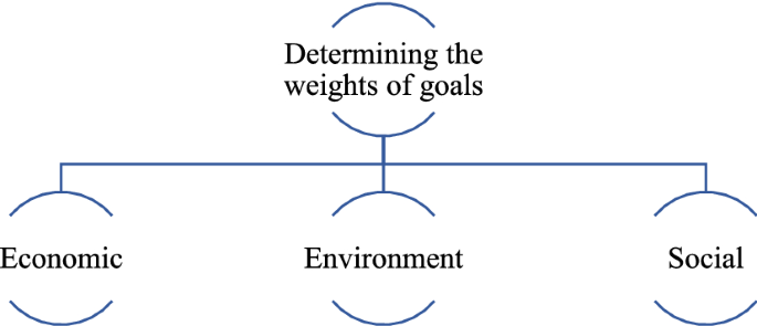

  

  Hierarchical structure for determining the weights of goals

• Step 2 Construct pairwise comparisons matrix

  The pairwise comparison matrices for the main criteria are determined by three experts using the linguistic scale in Table 9 (Kutlu Gündoğdu & Kahraman, 2020). The data were collected from three experts through a structured survey. Table 10 gives the experts’ opinions on the pairwise matrices of the main criteria.

  Table 10 Pairwise matrices for each expert’s opinion

  Aggregated fuzzy pairwise comparison matrix for the main criteria is constructed as per Table 11.

  Table 11 Aggregated evaluations of three experts on the main criteria

• Step 3 Estimate the spherical fuzzy global and local weights of criteria:

  Table 12 The spherical fuzzy weights of the criteria

  We use the SWAM operator given in Definition (v). The weighted arithmetic mean is used to compute the spherical fuzzy weights, as given in Table 12.

References

Abanades, S., Abbaspour, H., Ahmadi, A., Das, B., Ehyaei, M. A., Esmaeilion, F., & Bani-Hani, E. H. (2022). A critical review of biogas production and usage with legislations framework across the globe. International Journal of Environmental Science and Technology, 19(4), 3377–3400. https://doi.org/10.1007/s13762-021-03301-6
Abbasi, G., Khoshalhan, F., & Hosseininezhad, S. J. (2022). Municipal solid waste management and energy production : A multi-objective optimization approach to incineration and biogas waste-to-energy supply chain. Sustainable Energy Technologies and Assessments, 54, 102809. https://doi.org/10.1016/j.seta.2022.102809
Aboytes-Ojeda, M., Castillo-villar, K. K., & Eksioglu, S. D. (2022). Modeling and optimization of biomass quality variability for decision support systems in biomass supply chains. Annals of Operations Research, 314(2), 319–346. https://doi.org/10.1007/s10479-019-03477-8
Abraham, A., Mathew, A. K., Park, H., Choi, O., & Sindhu, R. (2020). Bioresource technology pretreatment strategies for enhanced biogas production from lignocellulosic biomass. Bioresource Technology, 301, 122725. https://doi.org/10.1016/j.biortech.2019.122725
Achinas, S., & Willem Euverink, G. J. (2020). Rambling facets of manure-based biogas production in Europe: A briefing. Renewable and Sustainable Energy Reviews, 119, 109566. https://doi.org/10.1016/j.rser.2019.109566
Ahmadvand, S., Khadivi, M., Arora, R., & Sowlati, T. (2021). Energy conversion and management : X Bi-objective optimization of forest-based biomass supply chains for minimization of costs and deviations from safety stock. Energy Conversion and Management: X, 11, 100101. https://doi.org/10.1016/j.ecmx.2021.100101
Ahmadvand, S., & Sowlati, T. (2022). A robust optimization model for tactical planning of the forest-based biomass supply chain for syngas production. Computers & Chemical Engineering, 159, 107693. https://doi.org/10.1016/j.compchemeng.2022.107693
Akhtari, S., Sowlati, T., Siller-Benitez, D. G., & Roeser, D. (2019). Impact of inventory management on demand fulfilment, cost and emission of forest-based biomass supply chains using simulation modelling. Biosystems Engineering, 178, 184–199. https://doi.org/10.1016/j.biosystemseng.2018.11.015
Aksay, M. V., & Tabak, A. (2022). Mapping of biogas potential of animal and agricultural wastes in Turkey. Biomass Conversion and Biorefinery, 12(11), 5345–5362.
Allman, A., Lee, C., Martín, M., & Zhang, Q. (2021). Biomass waste-to-energy supply chain optimization with mobile production modules. Computers & Chemical Engineering, 150, 107326. https://doi.org/10.1016/j.compchemeng.2021.107326
Amigun, B., & Von Blottnitz, H. (2010). Capacity-cost and location-cost analyses for biogas plants in Africa. Resources, Conservation and Recycling, 55(1), 63–73. https://doi.org/10.1016/j.resconrec.2010.07.004
Amore, F., & Bezzo, F. (2016). Strategic optimisation of biomass-based energy supply chains for sustainable mobility. Computers and Chemical Engineering, 87, 68–81.
Arabi, M., Yaghoubi, S., & Tajik, J. (2019). Algal biofuel supply chain network design with variable demand under alternative fuel price uncertainty : A case study. Computers & Chemical Engineering, 130, 106528. https://doi.org/10.1016/j.compchemeng.2019.106528
Aranguren, M., Castillo-Villar, K. K., & Aboytes-Ojeda, M. (2021). A two-stage stochastic model for co-firing biomass supply chain networks. Journal of Cleaner Production, 319, 128582. https://doi.org/10.1016/j.jclepro.2021.128582
Avcioǧlu, A. O., & Türker, U. (2012). Status and potential of biogas energy from animal wastes in Turkey. Renewable and Sustainable Energy Reviews, 16(3), 1557–1561. https://doi.org/10.1016/j.rser.2011.11.006
Azadeh, A., & Arani, H. V. (2016). Biodiesel supply chain optimization via a hybrid system dynamics-mathematical programming approach. Renewable Energy, 93, 383–403. https://doi.org/10.1016/j.renene.2016.02.070
Babazadeh, R., Razmi, J., Pishvaee, M. S., & Rabbani, M. (2017). A sustainable second-generation biodiesel supply chain network design problem under risk. Omega (united Kingdom), 66, 258–277. https://doi.org/10.1016/j.omega.2015.12.010
Bairamzadeh, S., Saidi-Mehrabad, M., & Pishvaee, M. S. (2018). Modelling different types of uncertainty in biofuel supply network design and planning: A robust optimization approach. Renewable Energy, 116, 500–517. https://doi.org/10.1016/j.renene.2017.09.020
Boro, M., Verma, A. K., Chettri, D., Yata, V. K., & Verma, A. K. (2022). Strategies involved in biofuel production from agro-based lignocellulose biomass. Environmental Technology and Innovation, 28, 102679. https://doi.org/10.1016/j.eti.2022.102679
Boulamanti, A. K., Maglio, S. D., Giuntoli, J., & Agostini, A. (2013). Influence of different practices on biogas sustainability. Biomass and Bioenergy, 53, 149–161.
Büyüközkan, G., & Güler, M. (2020). Analysis of companies’ digital maturity by hesitant fuzzy linguistic MCDM methods. Journal of Intelligent & Fuzzy Systems, 38(1), 1119–1132.
Cambero, C., Sowlati, T., & Pavel, M. (2015). Chemical engineering research and design economic and life cycle environmental optimization of forest-based biorefinery supply chains for bioenergy and biofuel production. Chemical Engineering Research and Design, 107, 218–235. https://doi.org/10.1016/j.cherd.2015.10.040
Can, A. (2022). Investigation of provincial capacity to produce biogas from waste disposal sites in Turkey. Energy, 258, 124778. https://doi.org/10.1016/j.energy.2022.124778
Charnes, A., Cooper, W. W., & Ferguson, R. (1955). Optimal estimation of executive compensation by linear programming. Management Science, 1, 138–151.
Charnes, A., & Cooper, W. W. (1961). Management models and industrial applications of linear programming. New York: Wiley.
Chen, C. W., & Fan, Y. (2012). Bioethanol supply chain system planning under supply and demand uncertainties. Transportation Research Part e: Logistics and Transportation Review, 48(1), 150–164. https://doi.org/10.1016/j.tre.2011.08.004
Chinese, D., Patrizio, P., & Nardin, G. (2014). Effects of changes in Italian bioenergy promotion schemes for agricultural biogas projects: Insights from a regional optimization model. Energy Policy, 75, 189–205. https://doi.org/10.1016/j.enpol.2014.09.014
Chyuan, H., & Silitonga, A.S. (2020). Patent landscape review on biodiesel production : Technology updates. Renewable and Sustainable Energy Reviews, 118(October 2019), 109526. https://doi.org/10.1016/j.rser.2019.109526
Cobuloglu, H. I., & Büyüktahtakin, I. E. (2014). A mixed-integer optimization model for the economic and environmental analysis of biomass production. Biomass and Bioenergy, 67, 8–23. https://doi.org/10.1016/j.biombioe.2014.03.025
Cooper, N., Panteli, A., & Shah, N. (2019). Linear estimators of biomass yield maps for improved biomass supply chain optimisation. Applied Energy, 253, 113526. https://doi.org/10.1016/j.apenergy.2019.113526
Corsano, G., Vecchietti, A. R., & Montagna, J. M. (2011). Optimal design for sustainable bioethanol supply chain considering detailed plant performance model. Computers and Chemical Engineering, 35(8), 1384–1398. https://doi.org/10.1016/j.compchemeng.2011.01.008
Čuček, L., Lam, H. L., Klemeš, J. J., Varbanov, P. S., & Kravanja, Z. (2010). Synthesis of regional networks for the supply of energy and bioproducts. Clean Technologies and Environmental Policy, 12(6), 635–645. https://doi.org/10.1007/s10098-010-0312-6
Čuček, L., Varbanov, P. S., Klemeš, J. J., & Kravanja, Z. (2012). Total footprints-based multi-criteria optimisation of regional biomass energy supply chains. Energy, 44(1), 135–145. https://doi.org/10.1016/j.energy.2012.01.040
DECC (Department of Energy & Climate Change), Government emission conversion factors for greenhouse gas company reporting: Conversion factors 2017
Díaz-trujillo, L. A., & Fabricio, N. (2019). Optimization of biogas supply chain in Mexico considering economic and environmental aspects. Renewable Energy, 139, 1227–1240. https://doi.org/10.1016/j.renene.2019.03.027
Dominique, L., Bambara, F., Sawadogo, M., Roy, D., Blin, J., Anciaux, D., & Koucka, S. (2019). Energy for sustainable development wild and cultivated biomass supply chain for biofuel production. A comparative study in West Africa. Energy for Sustainable Development, 53, 1–14. https://doi.org/10.1016/j.esd.2019.08.004
Egieya, J. M., Cu, L., Zirngast, K., Isafiadea, A. J., Pahorc, B., & Kravanja, Z. (2019). Synthesis of biogas supply networks using various biomass and manure types. Computers and Chemical Engineering, 122(2019), 129–151.
Elisabeth, L., Büsing, C., & Walther, G. (2018). Robust and sustainable supply chains under market uncertainties and different risk attitudes – A case study of the German biodiesel market. European Journal of Operational Research, 269, 302–312. https://doi.org/10.1016/j.ejor.2017.07.015
Fattahi, M., & Govindan, K. (2018). A multi-stage stochastic program for the sustainable design of biofuel supply chain networks under biomass supply uncertainty and disruption risk : A real-life case study. Transportation Research Part E, 118, 534–567. https://doi.org/10.1016/j.tre.2018.08.008
Ganesh, R., Torrijos, M., Sousbie, P., Lugardon, A., Steyer, J. P., & Delgenes, J. P. (2015). Effect of increasing proportions of lignocellulosic cosubstrate on the single-phase and two-phase digestion of readily biodegradable substrate. Biomass and Bioenergy, 80, 243–251. https://doi.org/10.1016/j.biombioe.2015.05.019
Ganev, E., Ivanov, B., Vaklieva-Bancheva, N., Kirilova, E., & Dzhelil, Y. (2021). A multi-objective approach toward optimal design of sustainable integrated biodiesel/diesel supply chain based on first-and second-generation feedstock with solid waste use. Energies, 14(8), 2261.
Gao, M., Wang, D., Wang, H., Wang, X., & Feng, Y. (2019). Biogas potential, utilization and countermeasures in agricultural provinces : A case study of biogas development in Henan Province, China. Renewable and Sustainable Energy Reviews, 99(May 2018), 191–200. https://doi.org/10.1016/j.rser.2018.10.005
Ge, Y., Li, L., & Yun, L. (2021). Modeling and economic optimization of cellulosic biofuel supply chain considering multiple conversion pathways. Applied Energy, 281, 116059. https://doi.org/10.1016/j.apenergy.2020.116059
Ghaderi, H., Pishvaee, M. S., & Moini, A. (2016). Biomass supply chain network design: An optimization-oriented review and analysis. Industrial Crops and Products, 94, 972–1000. https://doi.org/10.1016/j.indcrop.2016.09.027
Ghelichi, Z., Saidi-mehrabad, M., & Pishvaee, M. S. (2018). A stochastic programming approach toward optimal design and planning of an integrated green biodiesel supply chain network under uncertainty : A case study. Energy, 156, 661–687. https://doi.org/10.1016/j.energy.2018.05.103
Gital Durmaz, Y., & Bilgen, B. (2020). Multi-objective optimization of sustainable biomass supply chain network design. Applied Energy, 272, 115259. https://doi.org/10.1016/j.apenergy.2020.115259
Gonela, V., Zhang, J., & Osmani, A. (2015). Stochastic optimization of sustainable industrial symbiosis based hybrid generation bioethanol supply chains q. Computers & Industrial Engineering, 87, 40–65. https://doi.org/10.1016/j.cie.2015.04.025
Guo, C., Hu, H., Wang, S., Rodriguez, L. F., Ting, K. C., & Lin, T. (2022). Multiperiod stochastic programming for biomass supply chain design under spatiotemporal variability of feedstock supply. Renewable Energy, 186, 378–393. https://doi.org/10.1016/j.renene.2021.12.144
Habib, M. S., Omair, M., Ramzan, M. B., Chaudhary, T. N., Farooq, M., & Sarkar, B. (2022). A robust possibilistic flexible programming approach toward a resilient and cost-efficient biodiesel supply chain network. Journal of Cleaner Production, 366, 132752. https://doi.org/10.1016/j.jclepro.2022.132752
Halim, A., Razik, A., Seong, C., & Elkamel, A. (2019). A model-based approach for biomass-to- bioproducts supply Chain network planning optimization. Food and Bioproducts Processing, 118, 293–305. https://doi.org/10.1016/j.fbp.2019.10.001
Han, Y., Wang, L., & Kang, R. (2023). Influence of consumer preference and government subsidy on prefabricated building developer’s decision-making: A three-stage game model. Journal of Civil Engineering and Management, 29(1), 35–49.
Han, Y., Yan, X., & Piroozfar, P. (2022). An overall review of research on prefabricated construction supply chain management. Engineering, Construction and Architectural Management. https://doi.org/10.1108/ECAM-07-2021-0668
Hosen, M., Siddik, M., Alam, N., Miah, M., & Kabiraj, S. (2022). Biomass energy for sustainable development: evidence from Asian countries. Environment, Development and Sustainability. https://doi.org/10.1007/s10668-022-02850-1
Hosseinalizadeh, R., Khamseh, A. A., & Akhlaghi, M. M. (2019). A multi-objective and multi-period model to design a strategic development program for biodiesel fuels. Sustainable Energy Technologies and Assessments, 36, 100545. https://doi.org/10.1016/j.seta.2019.100545
IEA (2020) Renewables 2020: Analysis and forecast to 2025 https://www.iea.org/reports/renewables-2020. Accessed 1 Dec 2022
IEA (2022) Renewables 2022: Analysis and forecast to 2027 https://www.iea.org/reports/renewables-2022. Accessed 5 Jan 2023
Jensen, I. G., Münster, M., & Pisinger, D. (2017). Optimizing the supply chain of biomass and biogas for a single plant considering mass and energy losses. European Journal of Operational Research, 262(2), 744–758. https://doi.org/10.1016/j.ejor.2017.03.071
Jonker, J. G. G., Junginger, H. M., Verstegen, J. A., Lin, T., Rodríguez, L. F., Ting, K. C., & van der Hilst, F. (2016). Supply chain optimization of sugarcane first generation and eucalyptus second generation ethanol production in Brazil. Applied Energy, 173, 494–510. https://doi.org/10.1016/j.apenergy.2016.04.069
Kesharwania, R., Suna, Z., Daglia, C., & Xiong, H. (2019). Moving second generation biofuel manufacturing forward: Investigating economic viability and environmental sustainability considering two strategies for supply chain restructuring. Applied Energy, 242(2019), 1467–1496.
Keskin, T., Arslan, K., Karaalp, D., & Azbar, N. (2018). The Determination of the trace element effects on basal medium by using the statistical optimization approach for biogas production from chicken manure. Waste and Biomass Valorization, 0, 1–10. https://doi.org/10.1007/s12649-018-0273-2
Kremljak, Z. (2017). Economy of Biogas Plants, 0136–0143. https://doi.org/10.2507/28th.daaam.proceedings.018
Kristianto, Y., & Zhu, L. (2019). Platforms planning and process optimization for biofuels supply chain. Renewable Energy, 140, 563–579. https://doi.org/10.1016/j.renene.2019.03.072
Kulišić, B., Par, V., & Metzler, R. (2015). Calculation of on-farm biogas potential: A Croatian case study. Biomass and Bioenergy, 74, 66–78.
Kutlu Gündoğdu, F., & Kahraman, C. (2019). A novel fuzzy TOPSIS method using emerging interval-valued spherical fuzzy sets. Engineering Applications of Artificial Intelligence, 85, 307–323.
Kutlu Gündoğdu, F., & Kahraman, C. (2020). A novel spherical fuzzy analytic hierarchy process and its renewable energy application. Soft Computing, 24(6), 4607–4621.
Kwon, O., Kim, J., & Han, J. (2022). Organic waste derived biodiesel supply chain network: Deterministic multi-period planning model. Applied Energy, 305, 117847. https://doi.org/10.1016/j.apenergy.2021.117847
Lijó, L., González-García, S., Bacenetti, J., & Moreira, M. T. (2017). The environmental effect of substituting energy crops for food waste as feedstock for biogas production. Energy, 137, 1130–1143. https://doi.org/10.1016/j.energy.2017.04.137
Liu, W. Y., Lin, C. C., & Yeh, T. L. (2017). Supply chain optimization of forest biomass electricity and bioethanol coproduction. Energy, 139, 630–645. https://doi.org/10.1016/j.energy.2017.08.018
Lyng, K. A., & Brekke, A. (2019). Environmental life cycle assessment of biogas as a fuel for transport compared with alternative fuels. Energies, 12(3), 532.
María, M., Chavez, M., Costa, Y., & Sarache, W. (2021). A three-objective stochastic location-inventory-routing model for agricultural waste-based biofuel supply chain. Computers & Industrial Engineering, 162(December 2020), 107759.https://doi.org/10.1016/j.cie.2021.107759
Marvin, W. A., Schmidt, L. D., Benjaafar, S., Tiffany, D. G., & Daoutidis, P. (2012). Economic optimization of a lignocellulosic biomass-to-ethanol supply chain. Chemical Engineering Science, 67(1), 68–79. https://doi.org/10.1016/j.ces.2011.05.055
Miltner, M., Makaruk, A., & Harasek, M. (2020). Review on available biogas upgrading technologies and innovations towards advanced solutions. Journal of Cleaner Production, 161(2017), 1329–1337. https://doi.org/10.1016/j.jclepro.2017.06.045
Miret, C., Chazara, P., Montastruc, L., Negny, S., & Domenech, S. (2016). Design of bioethanol green supply chain: Comparison between first and second generation biomass concerning economic, environmental and social criteria. Computers and Chemical Engineering, 85, 16–35. https://doi.org/10.1016/j.compchemeng.2015.10.008
Mirkouei, A., Haapala, K. R., Sessions, J., & Murthy, G. S. (2017). A mixed biomass-based energy supply chain for enhancing economic and environmental sustainability benefits: A multi-criteria decision making framework. Applied Energy, 206, 1088–1101. https://doi.org/10.1016/j.apenergy.2017.09.001
Mottaghi, M., Bairamzadeh, S., & Pishvaee, M. S. (2022). A taxonomic review and analysis on biomass supply chain design and planning: New trends, methodologies and applications. Industrial Crops and Products, 180(September 2021), 114747. https://doi.org/10.1016/j.indcrop.2022.114747
Murillo-Alvarado, P. E., Guillén-Gosálbez, G., Ponce-Ortega, J. M., Castro-Montoya, A. J., Serna-González, M., & Jiménez, L. (2015). Multi-objective optimization of the supply chain of biofuels from residues of the tequila industry in Mexico. Journal of Cleaner Production, 108, 422–441. https://doi.org/10.1016/j.jclepro.2015.08.052
Namany, S., Al-Ansari, T., & Govindan, R. (2019). Optimisation of the energy, water, and food nexus for food security scenarios. Computers and Chemical Engineering, 129, 106513. https://doi.org/10.1016/j.compchemeng.2019.106513
Nunes, L.J.R., Causer, T.P., & Ciolkosz, D. (2020). Biomass for energy : A review on supply chain management models. Renewable and Sustainable Energy Reviews, 120(April 2019), 109658. https://doi.org/10.1016/j.rser.2019.109658
Ocak, S., & Acar, S. (2021). Biofuels from wastes in Marmara region, Turkey: Potentials and constraints. Environmental Science and Pollution Research, 28, 66026–66042.
Osmani, A., & Zhang, J. (2017). Multi-period stochastic optimization of a sustainable multi-feedstock second generation bioethanol supply chain−A logistic case study in Midwestern United States. Land Use Policy, 61, 420–450. https://doi.org/10.1016/j.landusepol.2016.10.028
Paolotti, L., Martino, G., Marchini, A., & Boggia, A. (2017). Biomass and bioenergy economic and environmental assessment of agro-energy wood biomass supply chains. Biomass and Bioenergy, 97, 172–185. https://doi.org/10.1016/j.biombioe.2016.12.020
Paulo, H., Azcue, X., Barbosa-Póvoa, A. P., & Relvas, S. (2015). Supply chain optimization of residual forestry biomass for bioenergy production: The case study of Portugal. Biomass and Bioenergy, 83, 245–256. https://doi.org/10.1016/j.biombioe.2015.09.020
Poeschl, M., Ward, S., & Owende, P. (2010). Prospects for expanded utilization of biogas in Germany. Renewable and Sustainable Energy Reviews, 14(7), 1782–1797. https://doi.org/10.1016/j.rser.2010.04.010
Rabbani, M., Saravi, N. A., Farrokhi-Asl, H., Lim, S. F. W. T., & Tahaei, Z. (2018). Developing a sustainable supply chain optimization model for switchgrass-based bioenergy production: A case study. Journal of Cleaner Production, 200, 827–843. https://doi.org/10.1016/j.jclepro.2018.07.226
Rajendran, K., Aslanzadeh, S., & Taherzadeh, M. J. (2012). Household biogas digesters—A review. Energies, 5(8), 2911–2942. https://doi.org/10.3390/en5082911
Raven, R. P., & Gregersen, K. H. (2007). Biogas plants in Denmark: Successes and setbacks. Renewable and Sustainable Energy Reviews, 11(1), 116–132.
Rodr, M. V. (2002). Meta-goal programming. European Journal of Operational Research, 136, 422–429.
Sadat, M., Mohseni, S., Hasanzadeh, M., & Saman, M. (2018). Moringa oleifera biomass-to-biodiesel supply chain design : An opportunity to combat deserti fi cation in Iran. Journal of Cleaner Production, 203, 313–327. https://doi.org/10.1016/j.jclepro.2018.08.257
Saghaei, M., & Dehghanimadvar, M. (2020). Optimization and analysis of a bioelectricity generation supply chain under routine and disruptive uncertainty and carbon mitigation policies, (October 2019), 2976–2999. https://doi.org/10.1002/ese3.716
Salehi, S., Mehrjerdi, Y. Z., Sadegheih, A., & Hosseini-Nasab, H. (2022). Designing a resilient and sustainable biomass supply chain network through the optimization approach under uncertainty and the disruption. Journal of Cleaner Production, 359, 131741.
Santibañez-Aguilar, J. E., Lozano-García, D. F., Lozano, F. J., & Flores-Tlacuahuac, A. (2019). Sequential use of geographic information system and mathematical programming for optimal planning for energy production systems from residual biomass. Industrial & Engineering Chemistry Research, 58(35), 15818–15837. https://doi.org/10.1021/acs.iecr.9b00492
Santibañez-Aguilar, J. E., Morales-Rodriguez, R., González-Campos, J. B., & Ponce-Ortega, J. M. (2016). Stochastic design of biorefinery supply chains considering economic and environmental objectives. Journal of Cleaner Production, 136, 224–245. https://doi.org/10.1016/j.jclepro.2016.03.168
Sarker, B. R., Wu, B., & Paudel, K. P. (2019). Modeling and optimization of a supply chain of renewable biomass and biogas : Processing plant location. Applied Energy, 239, 343–355. https://doi.org/10.1016/j.apenergy.2019.01.216
Scano, E. A., Asquer, C., Pistis, A., Ortu, L., Demontis, V., & Cocco, D. (2014). Biogas from anaerobic digestion of fruit and vegetable wastes: Experimental results on pilot-scale and preliminary performance evaluation of a full-scale power plant. Energy Conversion and Management, 77, 22–30. https://doi.org/10.1016/j.enconman.2013.09.004
Seyitoglu, S. S., Avcioglu, E., & Haboglu, M. R. (2022). Determination of the biogas potential of animal waste and plant location optimisation: A case study. International Journal of Energy Research, 46(14), 20324–20338.
Shabani, N., & Sowlati, T. (2016). A hybrid multi-stage stochastic programming-robust optimization model for maximizing the supply chain of a forest-based biomass power plant considering uncertainties. Journal of Cleaner Production, 112, 3285–3293. https://doi.org/10.1016/j.jclepro.2015.09.034
Sharifzadeh, M., Garcia, M. C., & Shah, N. (2015). Biomass and Bioenergy Supply chain network design and operation : Systematic decision- making for centralized, distributed, and mobile biofuel production using mixed integer linear programming ( MILP ) under uncertainty. Biomass and Bioenergy, 81, 401–414. https://doi.org/10.1016/j.biombioe.2015.07.026
Silva, J. O. V., Almeida, M. F., da Conceição Alvim-Ferraz, M., & Dias, J. M. (2018). Integrated production of biodiesel and bioethanol from sweet potato. Renewable Energy, 124, 114–120. https://doi.org/10.1016/j.renene.2017.07.052
Singh, P., & Kalamdhad, A. S. (2022). Assessment of agricultural residue-based electricity production from biogas in India: Resource-environment-economic analysis. Sustainable Energy Technologies and Assessments, 54, 102843. https://doi.org/10.1016/j.seta.2022.102843
Sözer, S.,& Yaldiz, O. (2011). Muz serası atıkları ve sığır gübresi karışımlarından mezofilik fermantasyon sonucu üretilebilecek biyogaz miktarının belirlenmesi üzerine bir araştırma. A research on determination of biogas production from mixture of banana greenhouse wastes and cattle ma, 24, 75–78 (in Turkish)
Statista, (2022). Global CO2 emissions related to energy, 1975–2021. https://www.statista.com/statistics/526002/energy-related-carbon-dioxide-emissions-worldwide/. Accessed 1 Dec 2022
Tamiz, M., Jones, D., & Romero, C. (1998). Goal programming for decision making: An overview of the current state-of-the-art. European Journal of Operational Research, 111(3), 569–581. https://doi.org/10.1016/S0377-2217(97)00317-2
Uddin, R., Shaikh, A. J., Khan, H. R., Shirazi, M. A., Rashid, A., & Qazi, S. A. (2021). Renewable energy perspectives of Pakistan and Turkey: Current analysis and policy recommendations. Sustainability, 13(6), 3349. https://doi.org/10.3390/su13063349
Verma, M. K., Shrivastava, R. K., & Tripathi, R. K. (2009). Evaluation of min-max, weighted and preemptive goal programming techniques with reference to mahanadi reservoir project complex. Water Resources Management, 24(2), 299–319. https://doi.org/10.1007/s11269-009-9447-9
Walla, C., & Schneeberger, W. (2008). The optimal size for biogas plants. Biomass and Bioenergy, 32(6), 551–557.
Wu, J., Zhang, J., Yi, W., Cai, H., Li, Y., & Su, Z. (2022). Agri-biomass supply chain optimization in north China: Model development and application. Energy, 239, 122374. https://doi.org/10.1016/j.energy.2021.122374
Yang, Y., & Chiclana, F. (2009). Intuitionistic fuzzy sets: Spherical representation and distances. International Journal of Intelligent Systems, 24(4), 399–420.
Yıldız, H. G., & Ayvaz, B. (2018). Waste biomass based energy supply chain network design. Journal of International Trade, Logistics and Law, 4(1), 126–137.
Yilmaz Balaman, Ş, & Selim, H. (2015). A decision model for cost effective design of biomass based green energy supply chains. Bioresource Technology, 191, 97–109. https://doi.org/10.1016/j.biortech.2015.04.078
Zeren, F., & Akkuş, H. T. (2020). The relationship between renewable energy consumption and trade openness: New evidence from emerging economies. Renewable Energy, 147, 322–329. https://doi.org/10.1016/j.renene.2019.09.006
Zhang, C., Xiao, G., Peng, L., Su, H., & Tan, T. (2013). The anaerobic co-digestion of food waste and cattle manure. Bioresource Technology, 129, 170–176. https://doi.org/10.1016/j.biortech.2012.10.138
Zhang, T., Wu, X., Shaheen, S. M., Abdelrahman, H., Ali, E. F., Bolan, N. S., & Rinklebe, J. (2022). Improving the humification and phosphorus flow during swine manure composting: A trial for enhancing the beneficial applications of hazardous biowastes. Journal of Hazardous Materials, 425, 127906. https://doi.org/10.1016/j.jhazmat.2021.127906
Author information
Authors and Affiliations
Corresponding author
Ethics declarations
Conflict of interest
The authors declare that they have no conflict of interest.
Additional information
Publisher's Note
Springer Nature remains neutral with regard to jurisdictional claims in published maps and institutional affiliations.