
Abstract
When assessing urban eco-environmental sensitive areas (Urban Eco-ESAs) by multi-criteria evaluation method, the widely used weighted linear combination method may inevitably lead to some factors of high sensitive value being neutralized by other factors of low sensitive value, resulting in the neglect of some eco-sensitive areas as a consequence, while on the other hand, Boolean OR combination method, which give a result of high sensitive value as long as any factor has the value of high sensitivity and thus ignore the mutual compensation mechanism among ecological factors, can lead to excessively wide ranges of the eco-sensitive areas. To overcome the defects of these two methods, the authors propose an Urban Eco-ESAs synthesized assessment method giving finely controlled priority to bottleneck factors, and relative model based on selective local encouraging variable weights combination. The method is able to increase the weights of some eco-bottleneck factors on the basis of a weight-changing function in synthesizing multiple factor assessments as long as their assessment values break the bottleneck threshold values, which can guarantee the eco-sensitive areas identified by bottleneck factors being embodied in the final result, while also retain the compensation effect of multiple ecological factors, which makes the results of the assessment more reasonable. In order to deliver this empirical research, Taogang Town in China, which is adjacent to Net lake wetland nature reserve area, has been used as an example to confirm the validity of the method and the model.
1 Introduction
Ecologically sensitive lands within the urban area, which play an essential role in maintaining ecological balance, and ensure urban environment and ecological security, are treated as the bottom line of urban development (Haigh 1990). However, due to the interference caused by urban development activities, these ecological lands have become more vulnerable, especially in the rapidly urbanizing countries, such as China. The rapid extension of urban land easily erodes ecological sensitive areas, therefore strongly threatening the safety of the urban ecological system. To protect these areas and to avoid negative influences from urban construction, Urban Eco-ESAs (Environmentally Sensitive Areas) has been researched and developed (Shen et al. 2011).
Urban Eco-ESAs are ecological elements or entities in and around the city which are of ecological significance to the urban environment but with poor capability of recovery if damaged in some way by urbanization (Ibid). Urban Eco-ESAs are special kind of ESA according to the classification made by Steiner et al. (2000) and can be divided into four types (Ibid), including:
- (1)
ecologically ESA which contain one or more significant natural elements;
- (2)
perceptual and cultural ESA that contain one or more significant scenic, recreational, archaeological, historic, or cultural resources;
- (3)
natural resource ESA that provide essential and natural resources to support development; and
- (4)
natural hazard ESA which may create disasters with development.
To identify the Urban Eco-ESAs for sustainable development and ecosystem protection, some evaluation methods have been gradually developed in China to support urban planning. These methods have been widely used to delineate the scope of Urban Eco-ESAs and urban growth boundaries for rational sustainable development. Currently, the mainstream evaluation methods used in Urban Eco-ESAs assessment are multi-criteria ones, which are similar to those used in ESAs, apart from the differences in the selection of criteria. The assessment process generally consists of 4 steps: (1) identifying the factors (criteria) significant to the ecological environment and constructing an assessment index system (Liu et al. 2015; Deng et al. 2018; Symeonakis et al. 2016); (2) assessing and producing maps for each factor that rank the environmentally sensitive values for every land unit, which usually are divided into five classes of not sensitive, slightly sensitive, moderately sensitive, highly sensitive and extremely sensitive (Zhang et al. 2011; Chen and Li 2012; Pan et al. 2012; Leman et al. 2016); (3) applying combination methods, which mainly are weighted linear combination(WLC) and Boolean OR combination, to synthesize all the partial analysis maps into an integrated one (Olafsdottir and Runnström 2009; Kawy and Belal 2011; Bahreini and Pahlavanravi 2013); (4) analyzing the integrated map and identifying the ESAs. (Gadgil et al. 2011; Saxena et al. 2007).
Among these steps, much attention is concentrated on the construction of an assessment index system, little has been on the combination method. More critically, it has been taken for granted that the combination would generate correct outcomes. However, our researches explore that different synthesizing methods can result in different, even conflicting outcomes, and different combination methods have different accessing logic.
For example, when using Boolean OR combination method (Vanet et al. 2010; Hsiang and Huang 1996), any unit which is evaluated as ‘sensitive’ by any criterion is treated as the bottleneck of the ecosystem, and the synthesized result is then regarded as ‘sensitive’ no matter what the other evaluation values may be from other criteria perspectives. It shows a strong bottleneck effect. This can lead to excessively wide ranges of the sensitive areas, while ignoring the mutual compensation mechanism among ecological factors. When using WLC method to synthesize multiple factors, high evaluation values in some criteria can be offset by low evaluation values of other criteria, which may result in concealing important sensitive areas. For instance, a site can be highly sensitive with respect to species protection, but not sensitive with respect to bio-diversity. When using WLC, if these two factors have the same weight, the integrated outcome will result in areas being identified only as slightly sensitive.
In principle, an ideal integrated model should be a combination of the above two methods, retaining the ESAs identified by each single factor as much as possible, while reflecting the combination of multiple factors to certain degree, thus showing the compensation mechanism and combination effect among ecological factors.
To address the weaknesses aforementioned, a variable weights combination (VWC) method has been recommended by some ecologists (Ying et al. 2007; Zhao et al. 2012). The principle of VWC can be summarized as that when some area is sensitive to single factor, the weight of the factor will be increased, and if the increased weight is big enough, the result may be close to that obtained from the Boolean OR combination. However, since other factors are still involved in the process of synthetization, they play certain roles in compensation, which results in a nonlinear combination.
The main purpose of this paper is to propose a delicate assessment method aimed at Urban Eco-ESAs based on VWC to improve the rationality of Urban Eco-ESAs recognition, which provides a flexible and detailed set of rules by selecting variable weight factors (i.e. bottleneck factors), and the thresholds of activating the variable weights (i.e. bottleneck positions); it thus highlights the bottleneck effects of the selected ecological bottleneck factors when being activated, while maintaining the ability of mutual compensation among all factors. In general, it is an Urban Eco-ESAs synthesized assessment method of giving finely controlled priority to bottleneck factors.
2 Contextualizing synthesized methods in ESAs assessment
Early combination approaches for ESAs analysis evolved from the sun-print overlay of Charles Elliot and Warren Manning (Miller and Charles 1993; McHarg 1969), transparent overlays of Jacqueline Tyrwhitt (Steinitz 1994) in the late nineteenth and early twentieth century. McHarg (1969), who was regarded as the precursor of ESAs analysis, advanced the overlay techniques designed to minimize environmental damages (Collins et al. 2001). These early methods can be catalogued into Ordinal Combination (Hopkins 1977). However, Ordinal Combination ignores the interdependence among factors, Hopkins (1977) then advocated the Logical Combination (Rules of Combination). The rules assign suitability to sets of combinations of types and are expressed in terms of verbal logic. From the mathematic view, Logical Combination can be catalogued into the Boolean overlay, which means all the criteria have to be combined by logical operators, such as intersection (AND) and union (OR). However, the Boolean overlay may result in a very hard AND or a very liberal OR and may not tradeoff between criteria (Jiang and Eastman 2000). Besides, all the above approaches give equal importance to all factors indifferently, while the actual significance of the factors is obviously different.
At present, the most frequently used combination method is weighted linear combination (WLC), which can overcome most of these limitations (Malczewski 2000, 2011; Carter and Rinner 2014). WLC weights the factors and aggregates them by weighted averaging, and the determination of the weights is mostly based on Analytic Hierarchy Process (AHP) (Moeinaddini et al. 2010; Le et al. 2015). The approach of AHP is to build a hierarchy of the factors, and thought pairwise comparison of the factors by decision makers and/or experts. This approach is able to derive a numerical weight or priority for each factor of the hierarchy.
The weighting equation is as follows:
where wj is the weight of the jth criterion; xij is the attribute value of the jth criterion associated with the ith location; n is the number of criteria. However, unlike the lack of the Boolean overlay, WLC is characterized by full tradeoffs and average risk, exactly halfway between the AND and OR operations, which may result in the omission of some important ESAs.
To control the degree of tradeoff, Ordered Weighted Averaging (OWA) was introduced to the combination process (Jiang and Eastman 2000; Malczewski et al. 2003). OWA not only emphasizes the differences in importance between each of the factors, but also the differences in values of each; therefore it can catch those factors with maximum or minimum values even when they are low weighted. OWA firstly orders the values in a descending way and then gives each value an extra weight by OWA operator according to its ordered position (e.g. giving the first ordered value, which is also the biggest one, an extra weight of 0.6; and extra weights of 0.1 to the other 4 values in left ordered. By doing so, it means the importance of all the factors except the one with the biggest value will be extremely declined). Finally by using the normalized product of the original weights and the extra weights as the final weights, and weighted averages the values, it is able to reach a combined result.
OWA involves two sets of weights of criterion importance weights and order weights. The formula is as follows: for a given set of n criteria maps, OWA is defined as a function OWA: IRn → IR that has associated with it a set of order weights v = v1, v2, …, vn such that vj∈[0, 1], j = 1, 2, …, n, and Σvj = 1. Given the set of attribute value xi1, xi2, …, xin associated with the ith location:
where zi1≥ zi2≥ ··· ≥ zin is the sequence obtained by (re)ordering the attribute value xi1, xi2, …, xin in a descending order; wj is the weight of the jth criterion (Malczewski et al. 2003).
OWA involves associating a weight, vj, with a particular ordered ‘position’ of the attribute value xi1, xi2, …, xin at the ith location. The first ordered weight, v1, is assigned to the highest attribute value for the ith location, v2 is associated with the next lower value for the same location, and so on. The main limitation of OWA in ESAs analysis is that the weighting process is hard to control, and the meaning of the result is hard to explain.
In summary, the aforementioned methods may not be necessarily suitable to all types of ESAs analysis. Boolean overlay is easy to conduct but lacks of tradeoff between criteria. Taking Boolean OR overlay as an example, the consequences of analysis may be the outcome of high sensitive value as long as any factor that is of the value of high sensitivity. This method may also ignore the mutual compensation mechanism among ecological factors. WLC is widely used and is able to overcome most of the limitations of Boolean overlay but may come to the other extreme that is full tradeoff. The outcome may inevitably lead to some factors of high sensitive value being neutralized by other factors of low sensitive value, resulting in the neglect of some eco-sensitive areas as a consequence. OWA is a valid method to control the degree of tradeoff but lacks of recognized, targeted OWA operators for ESAs analysis, and the meaning of the result is hard to explain.
Recently, ecologists have begun to introduce the ‘Variable Weighting Method’ to deal with this problem. The Variable Weighting Method was first proposed by Wang (1985), which considered the attribute values among various factors and highlights the significant distinctions between individual factors by augmenting the weights of the factors. Integrated evaluation of students’ achievements was taken as example when Yao and Li (2000) studied the method of Local Variable Weights. In order to find some professionals without obvious defects in any subject, they used the Variable Weight Method to increase the weights of subjects for which the score was higher than 90 or less than 60 to reach the purpose of punishment or reward.
Since the Variable Weight Method was proposed, scholars have undertaken many in-depth and extensive research studies. Li (1995, 1996) proposed the principle and axiomatic definition of Variable Weight Method and divided variable weights into three types, Penalty Variable Weight, Encouraging Variable Weight, and Mixed Variable Weight. Yao and Li (2000) further proposed axiomatic definition of the Local Variable Weight, and studied corresponding Local State Variable Weights. Li and Hao (2009) did an in-depth study on the variable weight effects of Local State Variable Weights, and proposed the concept of Pole Configuration, Weight Change Rate and Balanced Force, trying to find an effective way to reasonably choose Local State Variable Weights.
Due to the various Variable Weights Method discussed above, ecologists have made some progress in achieving initial results. When Gong et al. (2008) did his ecological security research in Guangzhou, he used the Local Penalty Variable Weight approach to determine weights. Shu et al. (2012) applied Local Penalty Variable Weights to ecological suitability evaluation to highlight the veto role of bottleneck factors. Guo (2014) applied Local Penalty Variable Weights to farmland ecological security warning to help identify the potential hazards influence agriculturally ecological security. These studies demonstrate the effectiveness of the Variable Weights Method. However, these studies mainly rely on the application of the existing generic Variable Weights Model, but ignoring proposing the dedicated Variable Weights Model that matches ecologically sensitivity evaluation. The generic model applies varies weights of all evaluation factors with no differences, thus failing to highlight the ecological role of specific bottleneck factors, and as a result, the model is not fine enough.
Besides, some frontier studies have used other Nonlinear Combination Methods based on the research in the Multiple Criteria Decision Making (MCDM) (Collins et al. 2001), including the Ideal Point Method (IPM), Grey Cluster, the Artificial Neural Network (ANN). IPM orders a set of alternatives on the basis of their separation from an ideal point which represents a hypothetical alternative (Pereira and Duckstein 1993) and generates complete sets of weights and ranks for each criterion. The method is simple in principle but is not affected by the number of evaluation criteria in ESAs assessment. It is then able to overcome some disadvantages arising from the lack of independence among criteria that affect traditional methods (Liu et al. 2014). The Grey Cluster method is a multi-dimensional grey evaluation one (Yue et al. 2015), which establishes the whitening function of the index, and classifies object into several grey categories to reflect the interval of the level index value (Zhang 2012). This method can analyze and evaluate under uncertain conditions with incomplete information and can reduce the amount of calculation in evaluation process in ESAs assessment. The method effectively reduces the convergence of results and improves the accuracy of classification in ESAs assessment (Tian et al. 2011). The ANN is an information processing system that imitates the structure and function of human brain (Lek and Guégan 1999). It can automatically summarize the functional relationship between data through learning and training and is able to build complex models and to solve them quickly. In ESAs assessment, ANN system with a strong approximation and fault-tolerant ability can avoid human impacts to a great extent. It is then able to achieve good analysis and prediction results (Jiang et al. 2012). However, these methods are basically still at the exploratory stage in ESAs assessment.
3 Methods
3.1 Assessment principle
Our method to assess Urban Eco-ESAs applies a multi-criteria based on VWC. In term of criterion factors, the eco-environmentally sensitive value is divided into 5 levels, {1, 3, 5, 7, 9}, representing not sensitive, low-sensitive, moderately sensitive, highly sensitive, extremely sensitive, respectively. For synthesizing purpose, a specialized VWC model is proposed, which can assign variable weight factors (i.e. bottleneck factors) and their variable weight thresholds (i.e. bottleneck positions) to represent finely controlled bottleneck effects.
The logic of the method is that, among all ecologic factors, some may play leading roles in the ecosystem. An area being assessed as certain sensitive level by any of these factors, its eco-environment is easy to collapse. These leading factors should then be regarded as ecological bottleneck factors, and their bottleneck effect should be activated when the assessment results exceed certain sensitive levels corresponding to their bottleneck positions. So, in our VWC methods, bottleneck factors are variable weight factors, and the bottleneck positions are their variable weight thresholds. For any ecological bottleneck factor whose evaluation value breaks its bottleneck position, its weight will be dynamically increased to ensure its priority and highlight the bottleneck effect, while none-bottleneck factors do not have this attribute.
For example, A, B, C, D, E are selected as five evaluation factors, among which A, C are bottleneck factors and their bottleneck position are at 7 (highly sensitive). The weight of 5 evaluation factors from A to E is {0.3, 0.1, 0.3, 0.2, 0.1}. For a plot of land, we evaluate it by each single factor and obtain a group of evaluation values {9, 3, 5, 5, 1}. With the Boolean OR method, the synthesized evaluation result is 9 (i.e. extremely sensitive), which shows no tradeoff and compensation between factors. With the WLC method, the synthesized evaluation result is 5.6, which is moderately sensitive. Obviously, the extremely sensitive result identified by Factor A has been neutralized. However, when using VWC method, as the evaluation value of bottleneck Factor A is 9, exceeding the bottleneck position, so the weight variation is activated, and the weight is increased to highlight the bottleneck effect. But the evaluation value of bottleneck Factor C is 5, which does not meet the bottleneck position, so the weight stays the same. Since the weight of bottleneck Factor A has been increased, the weights of other factors are decreased by the same proportion to guarantee the total weight stays 1. The weight matrix obtained after variation is {0.55, 0.05, 0.2, 0.15, 0.05}(for example) and the final evaluation result is 6.9, as highly sensitive, which not only ensures the bottleneck factor not to be ‘neutralized,’ but also reflects the combination effect of all factors on ecological environment.
3.2 Assessment model
To achieve the aforementioned function, a selective local encouraging VWC model is proposed as following:
- (1)
Variable weight synthesized equation
The synthesized model uses the form of Variable Weights Sum (Eq. 3), in which the weight is not fixed, but becomes variable weight vector W(X) after adjusting the weight. The variable weight vector can be obtained according to Eq. 4.
where M is the synthesized evaluation value, n is the number of factors, wj(X) is the weight of the jth factor after varying weight, xj is the evaluation value of the jth factor, X is the state vector (also called as configuration), which is the evaluation value of each factor and \(X = ( x_{1} ,x_{2} , \ldots ,x_{n} )\).
- (2)
Variable weight function
According to the aforementioned principle of variable weights, the variable weight vector e(X) depends on the original weight W of each factor, and the weight change obtained by the state vector X (called as state variable weight vector S(X)). We use the normalized Hadamard product of original weight W and state variable weight vector S(X) to get the variable weight vector W(X) (Eq. 4).
where wj(X) is the weight of the jth factor after varying weight, wj is the original weight of the jth factor, \(S_{\left( X \right)} = (S_{1\left( X \right)} , S_{2\left( X \right)} , \ldots S_{n\left( X \right)} )\) is the state variable weight vector.
The state variable weight vector S(X) is obtained by Eq. 5, using exponential function to obtain encouraging results.
where \(\alpha\) is the weight change strength, and \(\alpha > 0\), the bigger \(\alpha\) is, the bigger the change of weight will be, ej is the evaluation value of the jth factor, βj is the variable weight threshold value of the jth factor, I is the set of ecological bottleneck factors.
- (3)
Control of variable weight change
In order to obtain the suitable variable weight change strength \(\alpha\), this paper applies the research results of Li and Hao (2009) and introduces the concept of Δ, which means the maximum variable weight change rate of the bottleneck factor which has the minimum weight in pole configuration (i.e. half of the factors are the maximum state values, and the other half are the minimum state values). By derivation, there is a function relation between Δ and \(\alpha\) as shown in Eq. 6; therefore, appropriate value of \(\alpha\) can be solved by setting the maximum variable weight change rate Δ which has real meaning.
In the equation, m is the number of non-bottleneck factors, wk is the minimum weight value among bottleneck factors, Xk is the maximum state vector. If we rank bottleneck factors by weight: \(w_{1} \le \cdots \le w_{s - m} \le \cdots \le w_{n - m}\), n is the number of factors; when n is even number, s = n/2; when n is odd number, s = (n−1)/2.
During the process of determining Δ, it is necessary to ensure Eq. 6 is meaningful (i.e. when \(m \ge s,0 <\Delta < \frac{1}{{w_{k} }}\),when \(m < s,\,0 <\Delta < \frac{1}{{\mathop \sum \nolimits_{j = 1}^{s - m} w_{j} }}\)). Through trial and error, we find out that the maximum variable weight change rate ∆ generally takes 2–3, which is more appropriate. Meanwhile, the higher the value of ∆ is, the more prominent the bottleneck effect is. Since the actual configuration may be more extreme (e.g. the bottleneck factor which has the minimum weight has the maximum state value in the same time, while other factors have the minimum state value) so the actual maximum variable weight change rate may exceed the value of Δ.
3.3 Examples of assessment index system
Compared to the WLC, the index system of our VWC method has added two more parameters. One is whether the index factors are variable weight ones (i.e. bottleneck factors), the other one is the variable weight threshold value (i.e. bottleneck position). Two examples are provided as follow
Terrain factors: it includes slope, aspect, relative elevation, etc. These factors, which have significant impacts on ecological environment in mountainous and hilly environment, can be generally assigned as bottleneck factors in these areas. However, their bottleneck positions are different according to topographic relief because the change of topography may affect the level of sensitive ecological environment. For example, in hilly area, the bottleneck effect of slope on eco-environment may only emerge when the factor is rated as extremely sensitive; however, in mountainous area, the bottleneck effect may be significant when the factor is rated only as highly sensitive. Therefor the bottleneck positions for these two circumstances are the value of extremely sensitive and highly sensitive, respectively. Nevertheless, terrain factors are usually treated as non-bottleneck factors in flat areas such as wetland, plain and desert due to less influences to ecological sensitivity.
Water factors: it includes lake, river, wetland, pond, etc., and their buffers. Water is the source of life and is easily to be damaged because of its integrity and internal diffusion. Therefore, it is usually defined as bottleneck factor in all types of regions, but of different bottleneck positions. For example, water is extremely important in desert, so the bottleneck positions can be the value of moderately sensitive. However, water factors can be the value of extremely sensitive in mountainous area.
4 Case study
4.1 Brief introduction
Taogang town and Net-lake Wetland Nature Reserve Area are both located in Yangxin County, Hubei Province, China. Taogang town is located to the northwest of the Net-lake. The Net-lake wetland, a world-renowned for the habitat of rare animals such as the oriental white stork, black stork, and white crane, extends deeply into Taogang town and constitutes a pleasant hill–water–field pattern. It intertwines with forests and hills and forms a variety of lake-gorge landforms.
In this research, Taogang town and the surrounding areas are selected for evaluation (Fig. 1a), with a total area of 11.8 square kilometers and a population of about 3900 in 2018. At present, the township scale of Taogang, of 20.17 hectares of construction land area, is rather small. Currently, the economy in Taogang town, which mainly relies on agriculture and fish farming, is far below the average level in Yangxin County. In recent years, the local government has brought in a few industrial enterprises to promote economic development to some extent. However, the local government decided to consider the best uses of the local ecological resources to develop ecological agriculture and tourism at the same time. In this case, they identify the Urban Eco-ESAs in order to balance ecological protection and economic development. This research, applying Urban Eco-ESAs assessment method, intends to help local people to determine the Urban Eco-ESAs.

(Source: By Authors)
Study area, sample points, and assessment results of single factors. a Study area and sample points, b elevation, c slope, d aspect, e waters, f habitat types, g normalized vegetation index, h species richness, i flood risk
4.2 Index selection
Based on our VWC method and ecological characteristics of Taogang town, this research establishes the index system comprising eight ecological factors and employs AHP (Analytic Hierarchy Process) and Delphi to determine the original weight of factors. Since the research area composes of mixed zones of hills and wetlands, which of the risk of flood, and of the habitat of rare animals, most factors are defined as bottleneck factors, except the slope, because of its relatively small effect. The basic index system is as shown in Table 1.
4.3 Urban eco-ESAs assessment
-
(1)
Evaluation of single factors
Based on the evaluation criteria listed in Table 1, we set the 5 m × 5 m rectangle as the spatial unit, using GIS to evaluate the sensitivity level of the study area considering each single factor. The evaluation result is divided into five classes, with scores 1, 3, 5, 7, and 9, representing not sensitive to extremely sensitive. The evaluation results of eight single factors are as shown in Fig. 1b–i. By analyzing and comparing, on the one hand, we found that the factors which led to the evaluation results of highly sensitive or extremely sensitive level are mainly elevation, habitat types, species richness and water protection. On the other hand, the locations of highly sensitive and extremely sensitive areas are in the waterfront regions and forest with relatively high elevation.
-
(2)
Synthesized assessment
Afterwards, for each 5 m × 5 m basic spatial unit, we brought the evaluation value of single factors into Eqs. 5 and 4 to obtain the final weight of each factor after varying weight, and then obtained the synthesized evaluation value for each unit by Eq. 3.
After the above steps, we got the synthesized evaluation value which can be any number in the continuous interval [1, 9]. As it has been mentioned, we divided the sensitivity level into five classes (1, 3, 5, 7, 9), but we have not defined the ecological meaning of numbers between these levels. To solve this problem, we divide the interval of comprehensive evaluation value [1,9] into five classes by Equal Division Method and each span is 1.6, so we got the following sensitivity subdivision: 1 ≤ not sensitive ≤ 2.6; 2.6 < slightly sensitive ≤ 4.2; 4.2 < moderately sensitive ≤ 5.8; 5.8 < highly sensitive ≤ 7.4; 7.4 < extremely sensitive ≤ 9, and the result is as shown in Fig. 2a.
Fig. 2 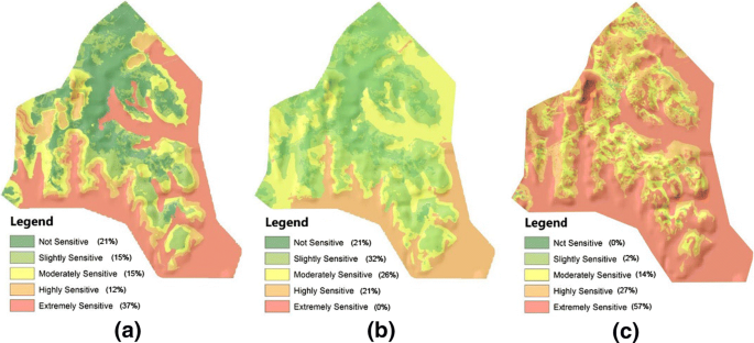
(Source: By Authors)
Assessment results of VWC, WLC, Boolean OR method. a VWC result, b WLC result, c Boolean OR result
To make a comparison, we also evaluated the study area with the method of WLC and Boolean OR based on the same index system and classification standards. Accordingly, the results are as shown in Fig. 2b, c.

4.4 Analysis of evaluation results
-
(1)
Overall analysis
The comparison of evaluation results with three methods is as shown in Fig. 2. The result of the WLC Method indicate that there are no extremely sensitive areas, only a few in highly sensitive category, accounting for 21% of the total research areas, which implies the tremendous impact of tradeoff effect (see Fig. 2b). On the contrary, the result of Boolean OR Method shows 57% of the research areas are extremely sensitive and no area is regarded as not sensitive, which is quite bipolar and does not match the real circumstances. However, the results of VWC Method neutralize these two methods to some degree, showing that 37% of the total research areas are extremely sensitive. Moreover, highly sensitive and extremely sensitive areas together take up 49% of the total research areas, which is twice of that determined by the WLC Method.
Comparing the WLC and the VWC Method, it reveals great differences when evaluating the wetland located in north-central, stretching deeply into the research areas from the east to the west. Despite being evaluated as extremely sensitive by many single factors, it is classified as moderately sensitive or mildly sensitive by the WLC Method, which is inconsistent with the real situation. In conclusion, when using WLC Method, extremely sensitive areas are often neutralized, which will affect the accuracy of delineation of urban ecologically sensitive areas.
-
(2)
Analysis of sample points
In this research, we selected three sample points which are representative to analyze the effect of VWC Method.
The locations of sample points are as shown in Fig. 1a, and the weight changes are as shown in Table 2.
Table 2 Weight changes of sample points.
Sample point B is in wetland area. This point is extremely sensitive in Habitat Types and Species Richness. The evaluation value of these two single factors both exceeds the bottleneck position. After varying weight, their weights are 2.5 times than their original weights. The synthesized evaluation value of point B is extremely sensitive, which is far more reasonable than that of WLC Method (moderately sensitive), and more according to practice.
Sample point C is in the South Lake. It is extremely sensitive or highly sensitive in Water, Habitat Types, Species Richness, and Flood Risk; the evaluation values of which all exceed bottleneck position, so the weight of 4 factors should be varied. However, there is a limitation that the total weight must be 1, which means the weights of these factors are not be able to be changed greatly. Thus, the variable weight change rates of these four factors are 1.8, 1.1, 1.75, 1.07, based on the standard that the higher the single factor evaluation value is, the greater the variable weight change rate is. The remaining four factors—Elevation, Slope, Aspect, Normalized Vegetation Index—since they did not involve in varying weight, their weights are greatly reduced to 0.02 or less, and their impact on the evaluation results is almost reduced to 0, which is consistent with subjective judgments, because these factors have no significance in sensitivity evaluation of the water area. Therefore, sample point C is defined as highly sensitive with WLC Method, while extremely sensitive with VWC Method.
In general, compared with the WLC and Boolean OR, the VWC Method can not only reflect the combination effect of ecological factors, but also highlight the importance of bottleneck factors, thus making the synthesis assessment results more reasonable.
4.5 Application of ecologically sensitive areas evaluation
The evaluation results show that highly and extreme highly sensitive areas account for 49% of the town, indicating that the township, though with excellent ecological resources, faces a tough problem on how to deal with the contradiction between ecological protection and urban construction during its development. It is time that planning and strict management should be established to protect the ecological environment and to avoid damage to the whole ecosystem.
For this reason, we define the areas of which the evaluation result is extremely sensitive or highly sensitive as ecologically sensitive parts in Taogang Town and include them in the scope of basic ecological areas. Meanwhile, assessment results are applied to the Master Planning of Taogang Town, mainly in the Land Suitability Evaluation and delineation of the Four Districts (i.e. prohibited-construction areas, restricted areas for construction, areas suitable for development and constructed areas).
In the Land Suitability Evaluation, the assessment results of Urban Eco-ESAs are involved as an important factor. And in the delineation of the four districts, the extremely sensitive areas and the highly sensitive areas are included in the prohibited-construction areas, the moderately sensitive areas are included in the restricted areas for construction, while a few moderately sensitive areas with great development value, as well as mildly sensitive areas and non-sensitive areas are clarified as the areas suitable for development.
5 Conclusion
This paper reconsiders the rationality of the quantitative synthesized assessment method of ESAs. By analyzing and comparing, we would argue the traditional synthesized evaluation method of Boolean OR shows extremely strong bottleneck effect, and on the other hand, the method of WLC cannot reflect ecological bottleneck effect of certain factors. Therefore, based on selective local encouraging variable weights combination (VWC) method, we propose an Urban Eco-ESAs synthesized assessment method giving finely controlled priority to bottleneck factors.
It is our argument that the effect of ecological bottleneck effect should not be ignored, however should be finely controlled as well. Firstly, only some of the factors are bottleneck factors, it depends on the eco-environment of the study area. Secondly, different bottleneck factors may have different bottleneck positions, the lower the bottleneck position is, the easier the bottleneck effect will be activated. Thirdly, during the process of multi-factor synthesization, the activated bottleneck effect should have the priority to be remained while the mutual compensation of all the factors should still be considered.
To fulfil this principle, the paper proposes a specialized VWC model, which can assign variable weight factors (i.e. bottleneck factors) and their variable weight thresholds (i.e. bottleneck positions) to represent finely controlled bottleneck effects. And accordingly, the index system of our assessment method adds two more parameters, bottleneck factors, and their bottleneck positions. This method can dynamically increase the weight of bottleneck factors according to its configuration, thereby highlighting the restriction role of ecological bottleneck factors, while retains the comprehensive effect of multiple ecological factors, thus making the evaluation results more reasonable.
Furthermore, Taogang Town has been used as an example to deliver an empirical research, confirming the effectiveness and feasibility of the method and model. According to our research, we suggest that the model should be further improved, especially the reasonable range of the Weight Change α. The establishment of the Index System of Urban Eco-ESAs Assessment is a complex and huge systematic project which should be further studied on ecological level. Besides the proposed VWC Assessment Method from this research can also be applied to Land Suitability Assessment, Environmental Landscape Evaluation, and similar evaluation existing bottleneck factors and buckets effect.
References
Bahreini, F., & Pahlavanravi, A. (2013). Assess and mapping the environmental sensitivity to desertification: A case study in Boushehr Province, Southwest Iran. International Journal of Agriculture and Crop Sciences,5(2), 172.
Carter, B., & Rinner, C. (2014). Locally weighted linear combination in a vector geographic information system. Journal of Geographical Systems,16(3), 343–361.
Chen, L., & Li, X. (2012). The ecological sensitivity evaluation in yellow river delta national natural reserve. Clean Soil, Air, Water,40(1), 197–1207.
Collins, M., Steiner, F., & Rushman, M. J. (2001). Land-use suitability analysis in the United States: Historical development and promising technological achievements. Environmental Management,28, 611–621.
Deng, W., Liu, D., Zhiyi, H. U., et al. (2018). Spatial difference of eco-environmental sensitivity of three gorges reservoir soil conservation area in Chongqing. Environmental Science and Technology,41(7), 190–198.
Gadgil, M., Ranjit, J., Ganeshaiah, K., Narendra, P. S., Murthy, M. S. R., Jha, C. S., et al. (2011). Mapping ecologically sensitive, significant and salient areas of Western Ghats: Proposed protocols and methodology. Current Science,100(2), 175–182.
Gong, J., Xia, B., & Chen, J. (2008). Spatially fuzzy assessment of regional eco-security in Guangzhou, a fast-urbanizing area: A case study in Guangzhou City. Acta Ecologicl Sinica,10, 4992–5001.
Guo, Y. (2014). Forewarning evaluation of farmland ecological security based on punished variable weight: A case of Xinjiang Production and Construction Corps. Areal Research and Development,5, 149–154.
Haigh, V. J. (1990). Environmentally sensitive areas. Landscape & Urban Planning,18(3), 235–239.
Hopkins, L. (1977). Methods for generating land suitability maps: A comparative evaluation. Journal of the American Institute of Planners,43, 386–400.
Hsiang, J., & Huang, G. S. (1996). Some fundamental properties of boolean ring normal forms. Dimacs,35, 587–602.
Jiang, H., & Eastman, J. R. (2000). Application of fuzzy measures in multi-criteria evaluation in GIS. International Journal of Geographical Information Science,14, 173–184.
Jiang, X. H., Liu, X., & Zhao, X. H. (2012). Research of wavelet neural networks in ecological sensitivity analysis—A case of hohhot city. Journal of Inner Mongolia Agricultural University,33(2), 189–192.
Kawy, W., & Belal, A. (2011). GIS to assess the environmental sensitivity for desertification in soil adjacent to El-Manzala Lake, East of Nile Delta, Egypt. American-Eurasian Journal of Agricultural & Environmental Sciences,10, 844–856.
Lek, S., & Guégan, J. F. (1999). Artificial neural networks as a tool in ecological modelling, an introduction. Ecological Modelling, 120(2), 65–73.
Lek, S., & Guégan, J. F. (1999). Artificial neural networks as a tool in ecological modelling, an introduction. Ecological Modelling,120(2–3), 65–73.
Leman, N., Ramli, M., & Khirotdin, R. (2016). GIS-based integrated evaluation of environmentally sensitive areas (ESAs) for land use planning in Langkawi, Malaysia. Ecological Indicators,61, 293–308.
Li, D., & Hao, F. (2009). Weights transferring effect of state variable weights vector Systems Engineering-Theory & Practice,29, 127–131.
Li, H. (1995). Factor spaces and mathematical frame of knowledge representation (VIII):variable weights analysis. Fuzzy Systems and Mathematics,9, 1–9.
Li, H. (1996). Factor spaces and mathematical frame of knowledge representation (IX):structure of balance functions and Weber–Fechner’s characteristics. Fuzzy Systems and Mathematics,10(12–17), 19.
Liu, J. H., Gao, J. X., Su, M. A., et al. (2015). Comprehensive evaluation of eco-environmental sensitivity in Inner Mongolia, China. China Environmental Science,35(2), 591–598.
Liu, R., Zhang, K., & Borthwick, A. (2014). Land-use suitability analysis for urban development in Beijing. Environmental Management,145(12), 170–179.
Malczewski, J. (2000). On the use of weighted linear combination method in GIS: Common and best practice approaches. Transactions in GIS,4(1), 5–22.
Malczewski, J. (2011). Local weighted linear combination. Transactions in GIS,15(4), 439–455.
Malczewski, J., Chapman, T., Flegel, C., Dan, S., & Healy, M. (2003). GIS–multi criteria evaluation with ordered weighted averaging (OWA): Case study of developing watershed management strategies. Environment and Planning A,35(10), 1769–1784.
McHarg, I. L. (1969). Design with nature. New York: American Museum of Natural History.
Miller, L., & Charles, E. (1993). Preservationist, park planner, and landscape architect. Pennsylvania: Department of Landscape Architecture, State College, Pennsylvania State University.
Moeinaddini, M., Khorasani, N., Danehkar, A., et al. (2010). Siting MSW landfill using weighted linear combination and analytical hierarchy process (AHP) methodology in GIS environment (case study: Karaj). Waste Management,30(5), 912.
Olafsdottir, R., & Runnström, M. (2009). A GIS approach to evaluating ecological sensitivity for tourism development in fragile environments. A case study from SE Iceland. Scandinavian Journal of Hospitality and Tourism,9, 22–38.
Pan, F., Tian, C., Feng, S., Zhou, W., & Chen, F. (2012). Evaluation of ecological sensitivity in Karamay, Xinjiang, China. Journal of Geographical Sciences,22(2), 329–345.
Pereira, J., & Duckstein, L. (1993). A multiple criteria decision-making approach to GIS-based land suitability evaluation. International Journal of Geographical Information Science,7, 407–424.
Saxena, M., Kumar, R., Saxena, P., Ra, N., & Jayanthis, S. (2007). Remote sensing and GIS based approach for environmental sensitivity studies: A case study from Indian Coast. International Society for Photogrammetry and Remote Sensing. http://www.isprs.org/proceedings/xxxv/congress/comm7/papers/225.pdf. Accessed February 10, 2016.
Shen, Q., Xu, S., Liu, L., & Qian, C. (2011). A new approach to the assessment of urban ecological sensitive area: The case of Songjian Lake district in Changzhou. Urban Planning Forum,193(1), 58–66.
Shu, B., Huang, Q., Liu, Y., & Yan, C. (2012). Spatial fuzzy assessment of ecological suitability for urban land expansion based on variable weights: A case study of Taicang. Journal of Natural Resources,27(3), 402–412.
Steiner, F., Blair, J., & Mcsherry, L. (2000). A watershed at a watershed: The potential for environmentally sensitive area protection in the upper san pedro drainage basin (Mexico and USA). Landscape & Urban Planning,49, 129–148.
Steinitz, C. (1994). A framework for theory and practice in landscape planning. Ekistics,4, 364–365.
Symeonakis, E., Karathanasis, N., Koukoulas, S., et al. (2016). Monitoring sensitivity to land degradation and desertification with the environmentally sensitive area index: The case of Lesvos Island. Land Degradation and Development,27(6), 1562–1573.
Tian, W. X., Zuo-Yong, L. I., & Liu, W. (2011). Grey clustering evaluation on regional eco-environmental quality based on normalized index value. Meteorological and Environmental Research,4, 65–67.
Vanet, A., Muller-Trutwin, M., & Valere, T. (2010). Method for identifying motifs and/or combinations of motifs having a boolean state of predetermined mutation in a set of sequences and its applications: US, US7734421.
Wang, P. (1985). Shadow of fuzzy sets and random set. Beijing: Beijing Normal University Press.
Yao, B., & Li, H. (2000). Axiomatic system of local variable weight. Systems Engineering-Theory & Practice,20(107–110), 113.
Ying, Z. S., Xin, L., & Ke, F. Z. (2007). Establishment of the changeable weight combination forecasting model and its application in regional ecological risk forecasting. Journal of Beijing Forestry University,29(2), 203–208.
Yue, L. I., Zhang, H., Zhang, X., et al. (2015). Evaluation on ecological security of urban land based on entropy method and grey prediction model. Environmental Science and Technology,38(12), 242–247.
Zhang, J., Wang, K., & Chen, X. (2011). Combining a fuzzy matter-element model with a geographic information system in eco-environmental sensitivity and distribution of land use planning. International Journal of Environmental Research & Public Health,8(4), 1206–1221.
Zhang, X. L. (2012). Application of projection pursuit dynamic cluster model in eco-environmental quality assessment. Advanced Materials Research,573–574, 256–259.
Zhao, G., Guo, S., Jing, S., et al. (2012). An investigation of coal demand in china based on the variable weight combination forecasting model. Journal of Resources & Ecology,2(2), 126–131.
Funding
Funding was provided by National Natural Science Foundations of China (Grant Nos. 51778503 and 1678393).
Author information
Authors and Affiliations
Corresponding author
Rights and permissions
Open Access This article is distributed under the terms of the Creative Commons Attribution 4.0 International License (http://creativecommons.org/licenses/by/4.0/), which permits unrestricted use, distribution, and reproduction in any medium, provided you give appropriate credit to the original author(s) and the source, provide a link to the Creative Commons license, and indicate if changes were made.
About this article

Cite this article
Niu, Q., Yu, L., Jie, Q. et al. An urban eco-environmental sensitive areas assessment method based on variable weights combination. Environ Dev Sustain 22, 2069–2085 (2020). https://doi.org/10.1007/s10668-018-0277-x
Received:
Accepted:
Published:
Issue Date:
DOI: https://doi.org/10.1007/s10668-018-0277-x