
Abstract
Weather and climate hazards cause too many fatalities each year. These weather and climate hazards are projected to increase in frequency and intensity due to global warming. Here, we use a disaster database to investigate continentally aggregated fatality data for trends. We also examine whether modes of climate variability affect the propensity of fatalities. Furthermore, we quantify fatality risk by computing effective return periods which depend on modes of climate variability. We find statistically significant increasing trends for heat waves and floods for worldwide aggregated data. Significant trends occur in the number of fatalities in Asia where fatalities due to heat waves and floods are increasing, while storm-related fatalities are decreasing. However, when normalized by population size, the trends are no longer significant. Furthermore, the number of fatalities can be well described probabilistically by an extreme value distribution, a generalized Pareto distribution (GPD). Based on the GPD, we evaluate covariates which affect the number of fatalities aggregated over all hazard types. For this purpose, we evaluate combinations of modes of climate variability and socio-economic indicators as covariates. We find no evidence for a significant direct impact from socio-economic indicators; however, we find significant evidence for the impact from modes of climate variability on the number of fatalities. The important modes of climate variability affecting the number of fatalities are tropical cyclone activity, modes of sea surface temperature and atmospheric teleconnection patterns. This offers the potential of predictability of the number of fatalities given that most of these climate modes are predictable on seasonal to inter-annual time scales.
1 Introduction
Extreme weather and climate events cause too many fatalities each year (e.g., Borden and Cutter 2008; Hoeppe 2016; Eckstein et al. 2019; Watts et al. 2019). These events cause on average 60,000 fatalities per year (Global Change Data Lab. Our World in Data 2019) (Fig. 1), which account for about 0.1% of all deaths globally on average; from year to year, this rate can range between 0.01 and 0.4%. While most fatalities occur in developing countries (Eckstein et al. 2019), developed countries can also experience deadly weather and climate events. For instance, in 2018, Germany ranked third in the annual Climate Risk Index of Germanwatch (Eckstein et al. 2019) because it was severely affected by drought conditions and a heat wave which caused about 1246 fatalities. The European heat wave of 2003 caused up to 70,000 fatalities (Robine et al. 2008). This shows that developed countries can also be severely affected by extreme events.

Mean and median numbers of fatalities due to weather and climate hazards: a worldwide, b Africa, c Asia, d Europe, e North America, f Central America, g South America and h Oceania
However, the most deadliest extreme weather and climate events occur in developing countries. Asia is the most affected continent; accounting for almost 70% of all fatalities in the period 1960 through 2019 based on the Emergency Events Database (EM-DAT) (Fig. 2). Africa is the second most affected, accounting for about 11%. Altogether, these events in developing countries account for almost 90% of all fatalities. Hence, an analysis of trends and whether the number of fatalities is potentially predictable is needed. Decreasing trends might suggest that societies were able to adapt to these events in order to mitigate their impacts or that our ability to predict and warn of these hazards has improved (Bakkensen and Mendelsohn 2016; Formetta and Feyen 2019).

Continental fractions of fatalities per year: a total number of fatalities and b number of fatalities per continental population
Fatal weather and climate extremes include heat waves (e.g., Gasparrini and Armstrong 2011; D’Ippoliti et al. 2010; Anderson and Bell 2010; Guo et al. 2017; Lee et al. 2019; Gasparrini et al. 2017), droughts (Ezra and Kiros 2000), storms (e.g., Brunkard et al. 2008; Diakakis et al. 2015; Rappaport 2014; Bakkensen and Mendelsohn 2016; Ashley and Gilson 2009), and floods (e.g., Jonkman and Kelman2005b; Jonkman 2005a; Kundzewicz and Kundzewicz 2005; He et al. 2018; Ashley and Ashley 2008; Doocy et al. 2013; Bouwer and Jonkman 2018). However, these types of extreme events are not necessarily independent from each other. Drought conditions are typically co-occurring with heat waves and storms can lead to flooding and other natural hazards. Hence, we have to deal with compound extremes (Leonard et al. 2014). One way to overcome potential difficulties in distinguishing between different types of extreme events is to aggregate over all of them to get more robust results. This will enable us to focus more on the large-scale drivers of these fatality events. Furthermore, aggregation of all hazard types is a sensible approach because the classification of fatalities to the different hazard types is non-trivial. For example, it is not always clear whether fatalities due to flooding which were caused by a storm has been attributed to the hazard type of flood or storm (Jonkman 2005a; Ashley and Ashley 2008).
Future climate simulations project that these extremes will become more frequent and intense (Field et al. 2012, 2014; Stocker et al. 2013; Franzke 2017) and will likely increase the number of fatalities (Wang et al. 2019). Best studied is probably the link between temperature and fatalities (e.g., Gasparrini et al. 2015; Deschenes and Moretti 2009). Gasparrini et al. (2015) show that cold temperatures actually cause more fatalities than warm temperatures. This would imply that global warming should lead to a reduction in temperature-related fatalities. However, their “temperature–mortality association relative risk” curves (Gasparrini et al. 2015) show relative steep slopes for increasing temperatures, which suggests that in a globally warmer world the number of fatalities might also steeply rise.
Since weather and climate extreme events occur episodically, the number of fatalities due to these hazards also varies considerably from year to year. Consequently, natural modes of climate variability will also affect the propensity of weather and climate extreme events to occur and the number of fatalities they cause. While previous studies typically employed regression techniques for the analysis of fatalities, here we study the probabilistic relationship between fatality risk and modes of climate variability and socio-economic indicators because of the episodic nature of extreme events. We do this by using extreme value statistics. In particular, we fit a non-stationary generalized Pareto distribution (GPD). To account for possible non-stationarities, we use covariates for the parameters of the GPD. Our study will provide probabilistic prediction models for the number of fatalities which will allow us to identify the climate drivers of disasters.
We use probabilistic methods to measure fatality risk. Our extreme value statistical methods provide probabilities of a given number of fatalities to occur per year. These probabilities can be converted into return levels and corresponding return periods (Coles 2001). Return levels are the number of fatalities y one can expect to occur once every x-years. Since, as we will show below, the probabilities of the number of fatalities will depend on large-scale modes of climate variability, return levels are less meaningful. Thus, we will use effective return levels (Cooley 2009, 2013; Katz et al.2002; Rootzén and Katz 2013) to quantify the risks of fatalities. Effective return levels depend on covariates, such as large-scale modes of climate variability. The El Niño–Southern Oscillation (ENSO) (McPhaden et al. 2006) is an example of such a mode.
Fatality studies are most often hazard specific or event specific, making systematic analysis of fatalities from weather and climate extreme events difficult. For this purpose, we present here a systematic study of continental fatalities across different hazard types and also aggregated over all hazard types. The aggregation is necessary since for all hazard types and continents, there is not a sufficient amount of events available for a robust analysis using probabilistic methods. Furthermore, since we are examining annual fatalities, it makes sense to aggregate over all hazard types in order to get an aggregated risk estimate since, e.g., a negative ENSO phase leads not only to an enhanced propensity of storms (Allen et al. 2015) but also to an enhanced likelihood of drought conditions (Mo and Schemm 2008) in the USA. Since many integrated climate assessment models mainly represent large or aggregated economies, e.g., Europe (Nordhaus and Boyer 2000; Leimbach et al. 2010), continentally integrated fatality models could be seamlessly included in such models. Hence, aggregating over hazard types can be useful for risk management purposes.
Here we address the following research questions: (i) Are there significant continental trends in the number of fatalities due to weather and climate extreme events? (ii) Can the number of fatalities be modeled by an extreme value distribution? and (iii) Are modes of climate variability affecting the propensity of fatalities? In Section 2, we describe the data used and the analysis methods. In Section 3, we discuss our results: first a trend analysis and second an extreme value statistic analysis. In Section 4, we summarize our results and conclude.
2 Data and methods
2.1 Data
In this study, we are using data from the International Disaster Database EM-DAT from the Centre for Research on the Epidemiology of Disasters (Guha-Sapir et al. 2017) to analyze disaster data related to weather and climate extreme events. The quality of EM-DAT has been discussed and compared with commercial databases by Guha-Sapir and Below (2002) and is of high standards. In our study, we use the group “Natural” disasters and select the following sub-groups: climatological, meteorological, and hydrological disasters. In particular, we consider the hazard types storm, flood, heat wave and drought. EM-DAT includes all disasters from 1900 until the present, conforming to at least one of the following criteria:
-
10 or more people dead
-
100 or more people affected
-
The declaration of a state of emergency
-
A call for international assistance
We use data for the period 1960 through 2019 because for this period, socio-economic data is available for all continents. We also aggregate the fatality data into continent-wide estimates. We consider Africa, Asia, Europe, North America, Central America, South America and Oceania as continents. The country classification is based on the list of countries per continent provided by Guha-Sapir et al. (2017). The time series of the number of fatalities are displayed in Fig. 3.

Number of fatalities due to weather and climate hazards: a worldwide, b Africa, c Asia, d Europe, e North America, f Central America, g South America and h Oceania
We use the following modes of climate variability and socio-economic indicators as covariates:
-
Gross domestic product (GDP) from the World Bank: https://data.worldbank.org/indicator/NY.GDP.MKTP.PP.KD (last accessed: 8th April 2020). GDP is a monetary measure of the market value of all services and final goods produced over a specific time period in a country. For each country, we converted the GDP to international dollars using purchasing power parity rates and then aggregated the annual GDP over the respective continents.
-
Population per country from the World Bank: https://data.worldbank.org/indicator/SP.POP.TOTL (last accessed: 8th April 2020). Annual country-level population numbers are used and then aggregated over the respective continents.
-
Global mean surface temperature (GMST) from the HadCRUT 4.6.0.0 annual mean data set (Morice et al. 2012). The GMST are temperature anomalies (deg C) relative to the 1961–1990 mean period.
-
Global mean sea level time series is based on data from Church and White (2011) and AVISO data (https://www.aviso.altimetry.fr/en/data/products/ocean-indicators-products/mean-sea-level/products-images.html).
-
The accumulated cyclone energy (ACE) index combines intensity and duration for individual tropical cyclones by squaring the 6-hourly intensity estimates reported in the best-track database and integrating over individual life cycles or seasons partitioned according to basin or hemisphere (Maue 2011). We use the ACE for the following regions: North Atlantic (ACE), West Pacific (ACEWP), North East Pacific (ACENEP), North Indian Ocean (ACENIO), Northern Hemisphere (ACENH), Southern Hemisphere (ACESH) and Global (ACEGLOBAL) (Villarini and Vecchi 2012).
-
The Net Tropical Cyclone (NTC) activity index in the Atlantic sector is computed as the mean over the following normalized parameters: number of named storms, number of named storm days, number of hurricanes, number of hurricane days, number of intense hurricanes and number of intense hurricane days. Normalization is done by the climatological values (Gray et al. 1994; Klotzbach 2007).
-
Sea surface temperature (SST) modes computed as empirical orthogonal functions of global gridded SST (Messié and Chavez 2011). SST1 is associated with ENSO (Philander 1983), SST2 with the Atlantic Multidecadal Oscillation (AMO) (Knight et al. 2005), SST3 with the Pacific Decadal Oscillation (PDO) (Mantua and Hare 2002), SST4 with the North Pacific Gyre Oscillation (NPGO) (Di Lorenzo et al. 2008) and El Niño Modoki (Ashok et al. 2007), and SST5 with El Niño Modoki and SST6 with the Atlantic Niño (Zebiak 1993). These SST modes comprise the most important modes of SST variability which have typically significant impacts on the atmospheric circulation and extreme events on long time scales.
-
The most dominant atmospheric teleconnection patterns such as the North Atlantic Oscillation (NAO), the Pacific-North American (PNA) pattern and the Southern Annual Mode (e.g., Wallace and Gutzler 1981; Feldstein and Franzke 2017). These teleconnection patterns exert significant impact on extreme events (e.g., Feldstein and Franzke 2017).
The above data is available on the Climate Explorer web page https://climexp.knmi.nl/start.cgiunless otherwise stated.
2.2 Methods
For the statistical trend analysis, we use quantile regression (e.g., Koenker and Hallock 2001, 2017; Donner et al. 2012; Franzke 2015) which approximates quantiles of a response variable using linear programming via the simplex algorithm (Koenker and Hallock 2001). Linear quantile regression minimizes the following functional:
where \(\rho _{p}(u)=puI_{[0,\infty )}-(1-p)uI_{(-\infty ,0)}(u)\) is the check function, IA(u) = 1 if u ∈ A and otherwise 0 is the indicator function, n is the length of the time series y, x = (1,x)T, x is a vector of the time points, β denotes the regression coefficients to be estimated and p the pre-specified quantile. We use the R package quantreg by Koenker (2018). Quantile regression is also robust against outliers. This is of advantage in our study since some years have very large fatalities numbers and by using quantile regression these singular events do not exert a dominant impact on our trend estimates. Due to the episodic nature of the fatalities time series, we only fit linear trends. Nonlinear trends would likely lead to non-robust trend estimates and polynomial trend functions could be highly affected by individual extreme events.
We also use the non-parametric Mann-Kendall method to test for statistical significance of trends (Mann 1945; Kendall 1948; Hamed and Rao 1998; Franzke 2015). The Mann-Kendall test detects monotonic trends without the need to provide a specified trend function form. The Mann-Kendall test is also robust against individual extreme events (or outliers).
We use the GPD (Coles 2001; Beirlant et al. 2006) to probabilistically examine the fatality data. We follow the approach by Franzke and Czupryna (2019). The GPD is given by
with \(z=\frac {x-\mu }{\sigma }\), where μ denotes the location, σ the scale and ξ the shape parameters. We systematically selected thresholds above which the GPD parameters do not change any longer with respect to their uncertainty bounds (Coles 2001).
We also allow these parameters to be dependent on covariates COVi (Coles 2001; Franzke and Czupryna 2019):
in order to ensure the positivity of the scale parameter σ we perform a log-transformation \(\phi = \log (\sigma )\) and the covariates dependence is as follows:
We use the same thresholds as for the stationary GPD models. We also tested the sensitivity of the non-stationary models to the threshold and found little sensitivity (not shown). Furthermore, we simultaneously fit a Poison point process to model the threshold exceedances (Coles 2001; Gilleland and Katz 2016; Franzke and Czupryna 2019). The use of Poisson-GPD models allows us to compute effective return periods which depend on covariates (Cooley 2013; Rootzén and Katz 2013). Since the occurrence probabilities depend on covariates, standard return periods are less meaningful. For given values of the covariates we compute the corresponding return periods and return levels. We use the R package extRemes by Gilleland and Katz (2016) for the extreme value analysis. The stationary and non-stationary GPD models are fitted using a maximum likelihood estimator.
3 Results
In Fig. 1, we summarize the mean and median of fatalities for the continents and across the 4 types of considered hazards. The comparison between the mean and median reveals that individual events can have a large impact on the annual mean number of fatalities. For instance, while worldwide annual mean drought fatalities are about 36,000, the annual median is just 8.5. The highest annual mean fatalities due to drought occur in Africa and Asia, while the annual medians are 0. This basically means that at least in 50% of the years of our data no fatalities due to drought occurred while the annual means would predict fatalities on the order of 10,000 per year. This is also a strong motivation for our use of probabilistic methods for modeling the annual numbers of fatalities. The number of fatalities in most continents is also dominated by one hazard type, e.g., heat waves in Europe and storms in North America.
In Fig. 3, we display the time series of the number of fatalities per year. A clear episodic behavior is discernible. A pronounced feature for all continents is that a few years can suffer an enormous number of fatalities, while all other years experience a much smaller number of fatalities. This is the behavior we already inferred from the comparison between mean and median fatalities in Fig. 1. This shows that the above stated number of 60,000 fatalities per year on average can be misleading especially when it comes to aid plans. This calls for robust methods to search for possible trends and to perform a probabilistic approach for examining climate and socio-economic contributors to the number of fatalities.
Here we briefly discuss some of the most deadliest events based on the EM-DAT database: Droughts are the cause of most fatalities in Africa. The 1983 drought in Ethiopia caused about 450,500 fatalities. River floods can also cause larger numbers of fatalities in Africa. The deadliest events in Asia occurred in India in 1965 with 1.5 million fatalities due to a drought. Bangladesh is often hit by storms due to which in 1970 about 300,000 people died. In Asia, droughts and tropical cyclones cause most fatalities on average. In Europe, heat waves are a major cause of fatalities; the 2003 heat wave in Italy, France and Spain caused large numbers of fatalities on the order of 70,000 (Robine et al. 2008) while the 2010 drought and heat wave in Russia led to about 55,000 fatalities. Since the fatalities are distributed among different European countries, the numbers of these events are ranked lower in disaster databases than if they happened in large countries. In North America, the deadliest event occurred in 2005 due to hurricane Katrina with about 1900 deaths. Most fatalities in North America are due to tropical cyclones, heat waves and convective storms. In Central America, hurricane Mitch killed over 11,000 people in 1998. Most fatalities in Central America are caused by tropical cyclones. In South America, the deadliest event was in 1999 in Venezuela due to a flash flood killing about 30,000. Flooding and land slides are the events causing the most fatalities in South America. The highest number of fatalities for Oceania is 600 due to a drought in Australia in 1967. The 2009 heat wave led to 347 deaths in Australia. In addition, tropical storms can also cause many fatalities in Oceania.
On average, extreme events account for 10.9% of Africa’s, 69.7% of Asia’s, 6.8% of Europe’s, 3.1% of North America’s, 3.4% of Central America’s, 5.4% of South America’s and 0.7% of Oceania’s yearly average fatalities due to weather and climate extreme events (Fig. 2a). However, this does not take into account the total population size of each continent. The fractions change once we divide the number of fatalities by the population size of the respective continent. After this, Africa accounts for 12.5%, Asia for 28.6%, Europe for 8.4%, North America for 9.1%, Central America for 13.9%, South America for 12.6% and Oceania for 14.9% of the yearly fatalities on average (Fig. 2b). This reveals that Asia is the most affected continent when it comes to fatalities both in total numbers and as a share of its population. Similarly, Oceania and Central America are severely affected when it comes to the number of fatalities per population. This is consistent with the fact that many countries from both continents are consistently ranked as extremely vulnerable to extreme weather and climate events by climate risk indices (Eckstein et al. 2019; Mucke et al. 2019).
3.1 Trends
Next, we investigate the fatality time series for trends. We focus on the mean and the 50th and 90th percentiles in order to detect possible trends in the mean, the median and a large quantile. Our results are displayed in Fig. 4 (see also Table S1). Our results reveal that significant trends occur in Asia and Africa. While in Asia the total number of fatalities experienced significant decreasing trends in both mean and median, this is mainly due to a reduction in fatalities due to storms. On the other hand, Asia suffers increasing numbers of fatalities due to floods and heat waves. Africa suffers from significant increases in overall fatalities which are mainly due to a significant increase in fatalities due to storms. Europe also suffers from an overall increase in fatalities which is mainly due to heat waves. This increase in Europe can be linked to recent heat waves which caused large-scale increases in fatalities during particular events (Robine et al. 2008; D’Ippoliti et al. 2010; Mitchell et al. 2016; Eckstein et al. 2019). The increase in European heat wave deaths has been attributed to global warming (Mitchell et al. 2016). Considering worldwide data, there are significant increases in fatalities due to heat waves and floods. Significant trends in extreme high numbers of fatalities are detectable in Asia and South America for heat waves where they are increasing, and in Europe for floods where they are decreasing. Considering that there are large population increases in some continents (not shown), we also examine whether there are trends in the number of fatalities as a fraction of the total population. Such an examination reveals that there are no significant trends. This shows that while the absolute number of fatalities is increasing for many hazards and continents, as a fraction of the total population, they are not significantly changing. This suggests that most societies are successfully mitigating the effects of extreme events (Bakkensen and Mendelsohn 2016; Formetta and Feyen 2019).

Schematic of continental trends of number of fatalities for different hazard types. 50th denotes the 50th percentile trend, 90th the 90th percentile trend and Mean the Mann-Kendall trend
3.2 Extreme value analysis
The episodic behavior visible in the fatality time series (Fig. 3) necessitates the use of probabilistic methods for a detailed analysis of the data. For this purpose, we use extreme value theory and fit a GPD to the time series. We start by fitting stationary GPD models to the continent-wide aggregated data for the different hazard types and for the aggregation of all hazard types. The quality of the GPD fits is evaluated using quantile-quantile plots (Coles 2001; Gilleland and Katz 2016; Franzke and Czupryna 2019). These plots demonstrate the goodness of fit of the GPD to the data (Fig. S1). For most quantiles, the GPD follows the data closely; thus, the points are close to the solid line; there are deviations visible only for very large values. These deviations are to be expected since for large quantiles only a very small number of observations are available and, thus, the variance increases. Overall, the GPD provides a good fit to the data and, therefore, allows us to compute return levels as a measure of fatality risk, which are given in Fig. 5. For drought, we were not able to estimate return periods due to a lack of sufficient data for Europe, North, Central, South America and Oceania. For Oceania, we also did not have sufficient data to compute return periods for heat waves. However, overall the stationary GPD provides good and robust fits and return periods.

Return levels based on stationary GPD model: a worldwide, b Africa, c Asia, d Europe, e North America, f Central America, g South America and h Oceania
Next we examine whether including covariates improves the GPD fits. We do this for data which are aggregated over all hazard types. For many hazard types on some continents, we do not have sufficient data to get robust non-stationary GPD fits. Since our focus here is on a global view of fatality risks, we focus on data aggregated over all hazards. We do this for the period 1960 through 2017, since for some climate indices, more up to date data is currently not available. We also examine combinations of covariates; for computational reasons, we only use up to three different covariates. This already gives us about 5400 different combinations to consider. We also only consider linear covariate relationships. Nonlinear relationships would require longer time series in order to get robust results. We then use the Bayesian Information Criterion (BIC) to select the GPD model which fits the data best (Burnham and Anderson 2003; Franzke and Czupryna 2019). The best GPD models with their parameter dependencies and covariates are given in Table S2. Our results show that the best model for the respective continents is significantly superior to the second best models according to our model selection procedure based on the BIC criterion; i.e., the difference in BIC of the respective models is larger than 2 (Burnham and Anderson 2003) (not shown).
For the worldwide aggregated data a stationary GPD model provides the best fit model, while for all continents covariates improve the GPD model. The covariates which affect the number of fatalities are tropical cyclone activity (ACENIO, ACEWP, ACESH), sea surface temperature anomalies (SST1, SST2, SST3, SST4) and atmospheric teleconnection patterns (NAO and PNA). The corresponding GPD model parameters are given in Table S2.
In order to provide estimates of likely numbers of fatalities, we provide return levels for 10-, 25- and 50-year return periods in Fig. 5 for the stationary model. In Table S3, we provide effective return levels based on the non-stationary models. To compute the effective return levels, we use the 10th, 50th and 90th percentiles of the respective quantiles and their combinations.
For Africa, the highest fatality risk is associated with a high state of the ACENIO index and negative states of the SST2 and NAO indices. ACENIO is generally an indicator of increased tropical cyclone landfall in east Africa (Fitchett and Grab 2014) while SST2, which corresponds to the AMO, and the NAO affect the propensity of drought conditions in Africa (McHugh and Rogers 2001; Knight et al. 2006; Ogunjo et al. 2019; Nigam and Ruiz-Barradas 2016). An example of a tropical cyclone hitting Africa is storm Idai, which formed over the Indian Ocean, in March 2019 and caused about 1303 fatalities (Benfield 2019).
For Asia the deadliest combination is a high ACEWP state and a negative PNA. Both lead to increased numbers of typhoons affecting East Asia. The negative phase of the PNA leads also to increases in the number of typhoons (Choi and Moon 2013; Song and Klotzbach 2019). Furthermore, the number of typhoons can also be seen as a proxy for both SST1/ENSO and SST3/PDO whose interplay affects typhoon activity (e.g., Elsner and Liu 2003; Zhao and Wang 2016). The interplay of ENSO with the PDO also affects drought and wet conditions (Wang et al. 2014; Krishnan and Sugi 2003). Hence, our results suggest that the ACEWP index might be an efficient proxy for this complex relationship with respect to the number of fatalities in this region.
For Europe, the deadliest combination is for negative SST1/ENSO and negative NAO states together with a high SST3/PDO state. The fact that a negative NAO state increases the propensity of European heat waves has been shown in Alvarez-Castro et al. (2018). An inspection of the SST1/ENSO index reveals that European heat waves have a higher propensity to occur during negative ENSO phases. The 2010 Russian heat wave has also occurred during negative SST1/ENSO and NAO phases (Trenberth and Fasullo 2012; Schneidereit et al. 2012). However, the ENSO-European heat wave is so far not well established and the role of the PDO in Europe is even less well studied. Thus, further research is needed.
North American fatalities are affected by negative SST1 and a positive PNA. SST1 is related to ENSO and a negative ENSO state has been linked to heat wave and drought conditions (Schubert et al. 2016) and increased numbers of hurricanes (Saunders et al. 2000). Also a positive PNA index is linked to drought conditions (Piao et al. 2016).
The number of fatalities in Central America is linked to the negative SST1/ENSO and the negative SST3/PDO. Negative ENSO state leads to an increase in hurricane landfalls (Saunders et al. 2000) and negative PDO states to an increase in flooding in Central America (Aguilar et al. 2005). Storms, flooding and land slides are the major causes of weather-related fatalities in Central America.
South America is affected by a positive SST1 state corresponding to a warm ENSO phase which is related to precipitation extremes and flooding (Grimm and Tedeschi 2009; del Rosario Prieto 2007); especially river flooding (Depetris et al. 1996; Pasquini and Depetris 2010).
Oceania is affected by SST4. SST4 is related to El Niño Modoki which can lead to drought conditions (Taschetto and England 2009) and heat waves (Loughran et al. 2017; Risbey et al. 2018).
A close inspection of the effective return levels (Table S3) reveals that for Asia, North and Central America, minimum fatality return levels are not given by the opposite percentile values as for the maximum fatality numbers. For instance, Asia exhibits the highest effective return levels for the 90th percentile of ACEWP and the 10th percentile of the PNA index, while the minimum effective return levels are given for the 90th percentile for both ACEWP and PNA. This indicates nonlinear behavior for these three continents since for linear behavior one would expect that the opposite percentile values (the opposite to the 90th is the 10th percentile) to maximum fatalities would produce minimum fatalities. In this respect, the other continents exhibit a more linear behavior.
4 Conclusions
We have performed a trend and a probabilistic analysis of continentally aggregated fatality data in which we aimed to address 3 research questions:
-
Are there significant continental trends in the number of fatalities due to weather and climate extreme events? We find statistically significant increasing trends for heat waves and floods for worldwide aggregated data. Significant trends occur in the number of fatalities in Asia where fatalities due to heat waves and floods are increasing while storm-related fatalities are decreasing. However, in Europe, we find the opposite; here, caused by recent heat waves, we find a significant upward trend in the number of fatalities due to heat waves and a significant downward trend for fatalities due to flooding. This suggests that Europe still needs to better adapt to heat waves and other natural hazards, whose frequency and intensity are projected to increase due to anthropogenic global warming in the future (Schoetter et al. 2015).
However, when normalized by population size, the trends are no longer significant. We did not find any evidence that population is a significant covariate. Whether and how population growth indirectly affects the total number of fatalities needs further research.
Overall, the numbers of fatalities over all hazard types are going down (see worldwide fatalities in Fig. 1); though, they are not statistically significant. This suggests that at least for storms and drought events most societies are better adapted (Bakkensen and Mendelsohn 2016). For storms, this might be due better forecasts and warnings.
The used fatality record is rather short, especially for analyzing extremes. Some of our considered climate covariates vary on fairly long time scales (e.g., Atlantic Multidecadal Oscillation, Pacific Decadal Oscillation); thus, they can also affect the long-term behavior of the number of fatalities. To distinguish better between forced trends and natural long-term variability, we need better and longer fatality data sets.
The analysis of extreme events can be strongly affected by single very extreme events, such as the drought event in India in 1965 with 1.5 million fatalities. However, our used trend estimation methods, such as quantile regression and the Sen slope, are robust with regard to extreme events (or outliers) (Koenker 2017; Shah et al. 2016).
-
Can the number of fatalities be modeled by an extreme value distribution? Our results demonstrate that the number of fatalities can be well described with a GPD. We also find evidence that for most continents, non-stationary GPD models perform better than stationary ones. Our results suggest that probabilistic approaches could be more suitable for modeling and predicting the number of fatalities than regression-based approaches. This can also be seen from the differences in the annual mean and median numbers of fatalities (Fig. 1) which shows that the mean can be dominated by a few very large events while most years have rather low numbers of fatalities.
-
Are modes of climate variability affecting the propensity of fatalities? We find clear evidence that modes of climate variability are affecting the propensity and number of fatalities on all continents. We showed that non-stationary GPDs provide good fits for continental fatality data. Significant covariates are the ENSO, the PDO, tropical cyclone activity, the NAO and PNA patterns. This is schematically displayed in Fig. 6. As these covariates are potentially predictable, this offers the potential to make probabilistic predictions of the number of fatalities.
Fig. 6 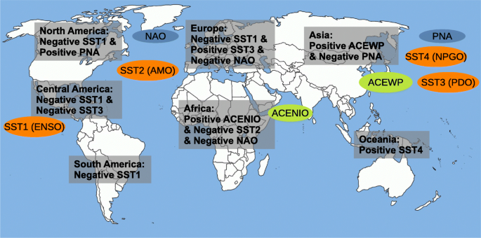
Schematic of climate modes and fatalities. Indicated is the sign of the covariates in order to lead to the highest risk of large numbers of fatalities to occur
Our results have the caveat that we aggregate for the probabilistic covariance analysis over all hazard types. This can potentially affect the physical interpretation of the results. On the one hand, the different hazard types might be forced by different covariates and aggregating over all of them might impede the identification of the physical causes. However, since for most continents just one hazard type is responsible for most of the fatalities, this seems not to be a large problem. Furthermore, aggregated fatality numbers will be useful for mitigation and adaptation actions. Moreover, the modes of climate variability also can affect different hazard types simultaneously, especially over the time period of 1 year. We also have discussed the known relationships between the modes of climate variability and hazards and have identified several relationships which have not been reported in the literature so far. However, the robustness of these relationships needs further research. It is also possible that indices such as tropical cyclone activity can act as a proxy for climate modes which have not been considered in our study.
Our analysis has found no direct evidence that anthropogenic global warming is affecting the number of fatalities since the global mean temperature is not a significant covariate for any of the continental fatalities time series. However, global warming might still indirectly affect the number of fatalities by, e.g., intensifying floods or storms. To make more definite statements about the role of anthropogenic global warming on mortality would require a systematic attribution study which is beyond the scope of this study. Nonetheless, the study by Mitchell et al. (2016) attributed fatalities caused by extreme heat to anthropogenic global warming. In particular, that study showed that anthropogenic global warming increased the risk of heat-related fatality by 70% in Paris and by 20% in London. However, adaptation can mitigate the number of fatalities during such weather- and climate-related events. For instance, the study by Bakkensen and Mendelsohn (2016) has shown that many nations were able to mitigate the impacts of tropical cyclones on mortality and economic damages.

Our results also show the potentially important role of the PDO in the propensity of weather and climate extremes. While there is a similarity with the spatial patterns of the ENSO, they operate on different time scales. Our results suggest their individual roles need to be better understood in order to make better predictions of extreme events. Our results will potentially enhance preparedness and disaster epidemiology (Noji 1995).
References
Aguilar E, Peterson T, Obando PR, Frutos R, Retana J, Solera M, Soley J, García IG, Araujo R, Santos AR et al (2005) Changes in precipitation and temperature extremes in Central America and northern South America. J Geophys Res 110(D23):1961–2003
Allen JT, Tippett MK, Sobel AH (2015) Influence of the el nino/southern oscillation on tornado and hail frequency in the united states. Nat Geosci 8(4):278–283
Alvarez-Castro MC, Faranda D, Yiou P (2018) Atmospheric dynamics leading to West European summer hot temperatures since 1851. Complexity
Anderson GB, Bell ML (2010) Heat waves in the United States: mortality risk during heat waves and effect modification by heat wave characteristics in 43 US communities. Environ Health Perspect 119(2):210–218
Benfield A (2019) Global Catastrophe Recap: First Half of 2019. http://thoughtleadership.aonbenfield.com//Documents/20190723-analytics-if-1h-global-report.pdf. Last accessed: 30.12.2019
Ashley ST, Ashley WS (2008) Flood fatalities in the united states. J Appl Meteorol Climatol 47(3):805–818
Ashley WS, Gilson CW (2009) A reassessment of us lightning mortality. Bull Amer Meteorol Soc 90(10):1501–1518
Ashok K, Behera SK, Rao SA, Weng H, Yamagata T (2007) El nino modoki and its possible teleconnection. J Geophys Res 112(C11)
Bakkensen LA, Mendelsohn RO (2016) Risk and adaptation: evidence from global hurricane damages and fatalities. J Assoc Environ Res Econ 3(3):555–587
Beirlant J, Goegebeur Y, Segers J, Teugels JL (2006) Statistics of extremes: theory and applications. Wiley, New York
Borden KA, Cutter SL (2008) Spatial patterns of natural hazards mortality in the United States. Int J Health Geograph 7(1):64
Bouwer LM, Jonkman SN (2018) Global mortality from storm surges is decreasing. Environ. Res Lett 13(1):014008
Brunkard J, Namulanda G, Ratard R (2008) Hurricane Katrina deaths, Louisiana, 2005. Dis Med Publ Health Pre 2(4):215–223
Burnham KP, Anderson DR (2003) Model selection and multimodel inference: a practical information-theoretic approach. Springer Science & Business Media
Choi K-S, Moon I-J (2013) Relationship between the frequency of tropical cyclones in Taiwan and the Pacific/North American pattern. Dyn. Atmos. Oceans 63:131–141
Church JA, White NJ (2011) Sea-level rise from the late 19th to the early 21st century. Surv Geophys 32(4-5):585–602
Coles S (2001) An introduction to statistical modeling of extreme values, vol 208. Springer, Berlin
Cooley D (2009) Extreme value analysis and the study of climate change. Clim Chang 97(1-2):77
Cooley D (2013) Return periods and return levels under climate change. In: AghaKouchak A, Easterling D, Hsu K, Schubert S, Sorooshian S (eds) Extremes in a changing climate. Springer, pp 97–114
del Rosario Prieto M (2007) ENSO Signals in South America: rains and floods in the Paraná river region during colonial times. Clim Chang 83(1-2):39–54
Depetris PJ, Kempe S, Latif M, Mook W (1996) Enso-controlled flooding in the Paraná river (1904–1991). Naturwissenschaften 83(3):127–129
Deschenes O, Moretti E (2009) Extreme weather events, mortality, and migration. Rev Econ Stat 91(4):659–681
Di Lorenzo E, Schneider N, Cobb KM, Franks P, Chhak K, Miller AJ, McWilliams JC, Bograd SJ, Arango H, Curchitser E et al (2008) North Pacific Gyre Oscillation links ocean climate and ecosystem change. Geophys Res Lett 35(8)
Diakakis M, Deligiannakis G, Katsetsiadou K, Lekkas E (2015) Hurricane Sandy mortality in the Caribbean and continental North America. Disaster Prev Manag 24(1):132–148
D’Ippoliti D, Michelozzi P, Marino C, De’Donato F, Menne B, Katsouyanni K, Kirchmayer U, Analitis A, Medina-Ramón M, Paldy A et al (2010) The impact of heat waves on mortality in 9 European cities: results from the euroHEAT project. Environ Health 9(1):37
Donner R, Ehrcke R, Barbosa S, Wagner J, Donges J, Kurths J (2012) Spatial patterns of linear and nonparametric long-term trends in Baltic sea-level variability. Nonlinear Proc Geophys 19(1):95–111
Doocy S, Daniels A, Murray S, Kirsch TD (2013) The human impact of floods: a historical review of events 1980-2009 and systematic literature review. PLoS Curr 5
Eckstein D, Künzel V, Schäfer L, Winges M (2019) Global climate risk index 2020, Who suffers most from extreme weather events? Weather-related loss events in 2018 and 1999 to 2018. Technical report, German Watch. http://germanwatch.org/sites/germanwatch.org/files/20-2-01e%20Global%20Climate%20Risk%20Index%202020_10.pdf. Last accessed: 04.12.2019
Elsner JB, Liu K-b (2003) Examining the ENSO-Typhoon hypothesis. Clim Res 25(1):43–54
Ezra M, Kiros G-E (2000) Household vulnerability to food crisis and mortality in the drought-prone areas of northern Ethiopia. J Biosocial Sci 32(3):395–409
Feldstein SB, Franzke CLE (2017) Atmospheric teleconnection patterns. In: Franzke CLE, O’Kane T (eds) Nonlinear and stochastic climate dynamics. Cambridge University Press, pp 54–104
Field CB, Barros V, Stocker TF, Dahe Q (2012) Managing the risks of extreme events and disasters to advance climate change adaptation: special report of the Intergovernmental Panel on Climate Change. Cambridge University Press
Field C, Barros V, Dokken D, Mach K, Mastrandrea M, Bilir T, Chatterjee M, Ebi K, Estrada Y, Genova R, Girma B, Kissel E, Levy A, MacCracken S, Mastrandrea P, White L (2014) Climate change 2014–impacts, adaptation and vulnerability: regional aspects. Cambrige University Press
Fitchett JM, Grab SW (2014) A 66-year tropical cyclone record for south-east Africa: temporal trends in a global context. I J Climatol 34(13):3604–3615
Formetta G, Feyen L (2019) Empirical evidence of declining global vulnerability to climate-related hazards. Glob Environ Chang 57:101920
Franzke CLE (2015) Local trend disparities of European minimum and maximum temperature extremes. Geophys Res Lett 42(15):6479–6484
Franzke CLE (2017) Impacts of a changing climate on economic damages and insurance. Econ Disaster Clim Chang 1(1):95–110
Franzke CLE, Czupryna M (2019) Probabilistic assessment and projections of US weather and climate risks and economic damages. Clim Chang:1–13
Gasparrini A, Armstrong B (2011) The impact of heat waves on mortality. Epidemiology 22(1):68
Gasparrini A, Guo Y, Hashizume M, Lavigne E, Zanobetti A, Schwartz J, Tobias A, Tong S, Rocklöv J, Forsberg B et al (2015) Mortality risk attributable to high and low ambient temperature: a multicountry observational study. Lancet 386(9991):369–375
Gasparrini A, Guo Y, Sera F, Vicedo-Cabrera AM, Huber V, Tong S, Coelho Md SZS, Saldiva PHN, Lavigne E, Correa PM et al (2017) Projections of temperature-related excess mortality under climate change scenarios. Lancet Planet Health 1(9):e360–e367
Gilleland E, Katz RW (2016) extRemes 2.0: an extreme value analysis package in R. J Stat Softw 72:1–39. https://doi.org/10.18637/jss.v072.i08
Global Change Data Lab. Our World in Data (2019) https://ourworldindata.org/natural-disasters. Last accessed: 2019-11-22
Gray WM, Landsea CW, Mielke Jr PW, Berry KJ (1994) Predicting atlantic basin seasonal tropical cyclone activity by 1 June. Wea Forecast 9(1):103–115
Grimm AM, Tedeschi RG (2009) ENSO and extreme rainfall events in South America. J Clim 22(7):1589–1609
Guha-Sapir D, Below R (2002) The quality and accuracy of disaster data: a comparative analyse of 3 global data sets. Technical Report 191, Disaster Management facility, World Bank, Working paper ID. https://dial.uclouvain.be/downloader/downloader.php?pid=boreal:179722&datastream=PDF_01. Last accessed: 22.03.2018
Guha-Sapir D, Hoyois P, Wallemacq P, Below R (2017) Annual disaster statistical review 2016. Technical report, Centre for Research on the Epidemology of Disasters (CRED). http://emdat.be/sites/default/files/adsr_2016.pdf. Last accessed: 12.01.2018
Guo Y, Gasparrini A, Armstrong B, Tawatsupa B, Tobias A, Lavigne E, Coelho Md SZS, Pan X, Kim H, Hashizume M et al (2017) Heat wave and mortality: a multicountry, multicommunity study. Environ Health Perspect 125(8):087006
Hamed KH, Rao AR (1998) A modified Mann-Kendall trend test for autocorrelated data. J Hydrol 204(1-4):182–196
He B, Huang X, Ma M, Chang Q, Tu Y, Li Q, Zhang K, Hong Y (2018) Analysis of flash flood disaster characteristics in China from 2011 to 2015. Nat Hazards 90(1):407–420
Hoeppe P (2016) Trends in weather related disasters–consequences for insurers and society. Wea Clim Extr
Jonkman SN (2005a) Global perspectives on loss of human life caused by floods. Nat Hazards 34(2):151–175
Jonkman SN, Kelman I (2005b) An analysis of the causes and circumstances of flood disaster deaths. Disasters 29(1):75–97
Katz RW, Parlange MB, Naveau P (2002) Statistics of extremes in hydrology. Adv Water Resour 25(8-12):1287–1304
Kendall MG (1948) Rank correlation methods. Griffin
Klotzbach PJ (2007) Recent developments in statistical prediction of seasonal Atlantic basin tropical cyclone activity. Tellus 59(4):511–518
Knight JR, Allan RJ, Folland CK, Vellinga M, Mann ME (2005) A signature of persistent natural thermohaline circulation cycles in observed climate. Geophys Res Lett 32(20)
Knight JR, Folland CK, Scaife AA (2006) Climate impacts of the Atlantic Multidecadal Oscillation. Geophys. Res Lett 33(17)
Koenker R, Hallock K (2001) Quantile regression: an introduction. J Econ Perspect 15(4):43–56
Koenker R (2017) Quantile regression: 40 years on. Ann Rev Econ 9(1):155–176. https://doi.org/10.1146/annurev-economics-063016-103651https://doi.org/10.1146/annurev-economics-063016-103651
Koenker R (2018) quantreg: quantile regression. https://CRAN.R-project.org/package=quantreg. R package version 5.35
Krishnan R, Sugi M (2003) Pacific Decadal Oscillation and variability of the Indian summer monsoon rainfall. Clim Dyn 21(3-4):233–242
Kundzewicz Z, Kundzewicz W (2005) Mortality in flood disasters. In Extreme weather events and public health responses. Springer, pp 197–206
Lee JY, Kim H, Gasparrini A, Armstrong B, Bell ML, Sera F, Lavigne E, Abrutzky R, Tong S, Coelho Md SZS et al (2019) Predicted temperature-increase-induced global health burden and its regional variability. Environ Int 131:105027
Leimbach M, Bauer N, Baumstark L, Luken M, Edenhofer O (2010) Technological change and international trade-insights from remind-r. Energy J 31(Special Issue)
Leonard M, Westra S, Phatak A, Lambert M, van den Hurk B, McInnes K, Risbey J, Schuster S, Jakob D, Stafford-Smith M (2014) A compound event framework for understanding extreme impacts. WIREs Clim Chang 5(1):113–128
Loughran TF, Perkins-Kirkpatrick SE, Alexander LV, Pitman AJ (2017) No significant difference between Australian heat wave impacts of Modoki and eastern Pacific El nino. Geophys Res Lett 44(10):5150–5157
Mann HB (1945) Nonparametric tests against trend. Econometrica:245–259
Mantua NJ, Hare SR (2002) The Pacific Decadal Oscillation. J Oceano 58(1):35–44
Maue RN (2011) Recent historically low global tropical cyclone activity. Geophys Res Lett 38(14)
McHugh MJ, Rogers JC (2001) North Atlantic Oscillation influence on precipitation variability around the southeast African convergence zone. J Clim 14 (17):3631–3642
McPhaden MJ, Zebiak SE, Glantz MH (2006) ENSO as an integrating concept in Earth science. Science 314(5806):1740–1745
Messié M, Chavez F (2011) Global modes of sea surface temperature variability in relation to regional climate indices. J Climat 24(16):4314–4331
Mitchell D, Heaviside C, Vardoulakis S, Huntingford C, Masato G, Guillod BP, Frumhoff P, Bowery A, Wallom D, Alle M (2016) Attributing human mortality during extreme heat waves to anthropogenic climate change. Environ Res Lett 11(7):074006
Mo KC, Schemm JE (2008) Relationships between ENSO and drought over the southeastern United States. Geophysical Research Letters, 35(15)
Morice CP, Kennedy JJ, Rayner NA, Jones PD (2012) Quantifying uncertainties in global and regional temperature change using an ensemble of observational estimates: The hadCRUT4 data set. J Geophys Res 117(D8)
Mucke P, Kirch L, Walter J (2019) World risk report 2019. Bündnis Entwicklung Hilft and UNU-EHS. https://weltrisikobericht.de/download/1243/. Last accessed: 24.09.2019
Nigam S, Ruiz-Barradas A (2016) Key role of the Atlantic Multidecadal Oscillation in 20th century drought and wet periods over the US Great Plains and the Sahel. In Dynamics and predictability of large-scale high-impact weather and climate events. Cambridge University Press, Cambridge
Noji EK (1995) Disaster epidemiology. J Med Sys 19(2)
Nordhaus WD, Boyer J (2000) Warming the world: economic models of global warming. MIT press
Ogunjo ST, Fuwape IA, Olusegun CF (2019) Impact of large scale climate oscillation on drought in West Africa. arXiv:1901.10145
Pasquini AI, Depetris PJ (2010) ENSO-triggered exceptional flooding in the Paraná River: where is the excess water coming from?. J Hydrol 383 (3-4):186–193
Philander SGH (1983) El Nino Southern Oscillation phenomena. Nature 302(5906):295–301
Piao L, Fu Z, Yuan N (2016) “Intrinsic” correlations and their temporal evolutions between winter-time PNA/EPW and winter drought in the west United States. Sci Rep 6:19958
Rappaport EN (2014) Fatalities in the United States from Atlantic tropical cyclones: new data and interpretation. Bull Amer Meteorol Soc 95(3):341–346
Risbey JS, O’Kane TJ, Monselesan DP, Franzke CL, Horenko I (2018) On the dynamics of austral heat waves. J Geophys Res 123(1):38–57
Robine J-M, Cheung SLK, Le Roy S, Van Oyen H, Griffiths C, Michel J-P, Herrmann FR (2008) Death toll exceeded 70,000 in Europe during the summer of 2003. Compt Rend Biol 331(2):171–178
Rootzén H, Katz RW (2013) Design life level: quantifying risk in a changing climate. Wat Resour Res 49(9):5964–5972
Saunders M, Chandler R, Merchant C, Roberts F (2000) Atlantic hurricanes and NW Pacific typhoons: ENSO spatial impacts on occurrence and landfall. Geophys Res Lett 27(8):1147–1150
Schneidereit A, Schubert S, Vargin P, Lunkeit F, Zhu X, Peters DH, Fraedrich K (2012) Large-scale flow and the long-lasting blocking high over Russia: summer 2010. Mon Wea Rev:2967–2981
Schoetter R, Cattiaux J, Douville H (2015) Changes of western European heat wave characteristics projected by the CMIP5 ensemble. Clim Dyn 45 (5-6):1601–1616
Schubert S, Stewart R, Wang H, Barlow M, Berbery E, Cai W, Hoerling M, Kanikicharla K, Koster R, Lyon B, Mariotti A, Mechoso C, Maeller O, Rodriguez-Fonseca B, Seager R, Senevirante S, Zhang L, Zhou T (2016) Global meteorological drought: a synthesis of current understanding with a focus on SST drivers of precipitation deficits. J Clim 29(11):3989–4019. https://doi.org/10.1175/JCLI-D-15-0452.1
Shah S, Rehman A, Rashid T, Karim J, Shah S (2016) A comparative study of ordinary least squares regression and Theil-Sen regression through simulation in the presence of outliers. J Sci Technol 137:142
Song J, Klotzbach PJ (2019) Relationship between the Pacific-North American pattern and the frequency of tropical cyclones over the western North Pacific. Geophys Res Lett 46:6118–6127
Stocker TF, Qin D, Plattner G-K, Tignor M, Allen SK, Boschung J, Nauels A, Xia Y, Bex V, Midgley PM (2013) Climate Change 2013: the physical science basis: Working Group I contribution to the Fifth Assessment Report of the Intergovernmental Panel on Climate Change. Cambridge University Press
Taschetto AS, England MH (2009) El Nino Modoki impacts on Australian rainfall. J Clim 22(11):3167–3174
Trenberth KE, Fasullo JT (2012) Climate extremes and climate change: the Russian heat wave and other climate extremes of 2010. J Geophys Res 117(D17). https://doi.org/10.1029/2012JD018020
Villarini G, Vecchi GA (2012) North Atlantic Power Dissipation Index (PDI) and Accumulated Cyclone Energy (ACE): Statistical modeling and sensitivity to sea surface temperature changes. J Clim 25(2):625–637
Wallace JM, Gutzler DS (1981) Teleconnections in the geopotential height field during the northern hemisphere winter. Mon Wea Rev 109(4):784–812
Wang S, Huang J, He Y, Guan Y (2014) Combined effects of the Pacific Decadal Oscillation and El Nino-Southern Oscillation on global land dry–wet changes. Sci Rep 4:6651
Wang Y, Wang A, Zhai J, Tao H, Jiang T, Su B, Yang J, Wang G, Liu Q, Gao C et al (2019) Tens of thousands additional deaths annually in cities of China between 1.5∘C and 2.0∘C warming. Nat Commun 10(1):1–7
Watts N, Amann M, Arnell N, Ayeb-Karlsson S, Belesova K, Boykoff M, Byass P, Cai W, Campbell-Lendrum D, Capstick S et al (2019) The 2019 report of The Lancet Countdown on health and climate change: ensuring that the health of a child born today is not defined by a changing climate. Lancet 394 (10211):1836–1878
Zebiak SE (1993) Air–sea interaction in the equatorial Atlantic region. J Clim 6(8):1567–1586
Zhao H, Wang C (2016) Interdecadal modulation on the relationship between ENSO and typhoon activity during the late season in the western North Pacific. Clim Dyn 47(1-2):315–328
Acknowledgments
We thank three anonymous reviewers for their comments which helped to improve this manuscript. We thank EM-DAT: The Emergency Events Database - Université Catholique de Louvain (UCL) - CRED, D. Guha-Sapir - www.emdat.be, Brussels, Belgium, for providing us with the fatality data.
Funding
Open Access funding provided by Projekt DEAL. This study was partially supported by the German Research Foundation (DFG) via the Collaborative Research Center TRR 181 – Projektnummer 274762653, DFG Grant FR3515/3-1 and the German Federal Ministry of Education and Research (BMBF) project ClimXtreme.
Author information
Authors and Affiliations
Corresponding author
Additional information
Publisher’s note
Springer Nature remains neutral with regard to jurisdictional claims in published maps and institutional affiliations.
Electronic supplementary material
Below is the link to the electronic supplementary material.
Rights and permissions
Open Access This article is licensed under a Creative Commons Attribution 4.0 International License, which permits use, sharing, adaptation, distribution and reproduction in any medium or format, as long as you give appropriate credit to the original author(s) and the source, provide a link to the Creative Commons licence, and indicate if changes were made. The images or other third party material in this article are included in the article's Creative Commons licence, unless indicated otherwise in a credit line to the material. If material is not included in the article's Creative Commons licence and your intended use is not permitted by statutory regulation or exceeds the permitted use, you will need to obtain permission directly from the copyright holder. To view a copy of this licence, visit http://creativecommons.org/licenses/by/4.0/.
About this article

Cite this article
Franzke, C.L.E., Torelló i Sentelles, H. Risk of extreme high fatalities due to weather and climate hazards and its connection to large-scale climate variability. Climatic Change 162, 507–525 (2020). https://doi.org/10.1007/s10584-020-02825-z
Received:
Accepted:
Published:
Issue Date:
DOI: https://doi.org/10.1007/s10584-020-02825-z