A robust method for clustering football players with mixed attributes

Abstract

A robust fuzzy clustering model for mixed data is proposed. For each variable, or attribute, a proper dissimilarity measure is computed and the clustering procedure combines the dissimilarity matrices with weights objectively computed during the optimization process. The weights reflect the relevance of each attribute type in the clustering results. A simulation study and an empirical application to football players data are presented that show the effectiveness of the proposed clustering algorithm in finding clusters that would be hidden unless a multi-attributes approach were used.

1 Introduction and literature review

Data in sports are being collected and analyzed, with the integration of physical and digital sources, increasing the knowledge of professional sports for all parties involved. Statistical methodology and data-driven analytics in sports can drive decision-making in different fields: marketing strategies, performances of players or teams, forecasting of revenues, health. Depending on the type of sport, on the nature of the data at hand, and on the objectives of the analysis, a variety of statistical learning and operations research methods has been proposed. In order to analyse the massive and the different kinds of sport data and their complex structure and then to capture their extensive information many advanced statistical methodologies, strategies of analyses and data-driven procedures have to be considered in the analysis process. In this way, managing this kind of data with advanced theoretical tools we obtain an informational gain and then the knowledge that represents the basis of any decision-making process in sport.

The playing characteristics of football players are important both from a technical and economic point of view. From the technical point of view they allow to evaluate the playing characteristics that lead the player and the team to achieve winning results; from the economic point of view they allow to establish the value of a player in the transfer market. Clustering of football players on the basis of playing characteristics, position and performance variables is relevant for clubs, either to drive team formation and selection of players, or for determining the value of a football player in the transfer window period (Behravan and Razavi 2021; Shelly et al. 2020; Narizuka and Yamazaki 2019).

Table 1 Some recent statistical papers on data in sport

In the literature, many empirical studies and methodological proposals based on data science and data-driven approach have been carried out on many sports disciplines to analyze the large mass of sport data both in the field of performance and in the medical, social or economic fields (Table 1). For instance, Palacios-Huerta (2004) analyses the effects of rules of the game of football using an econometric methodology for dating structural breaks in tests with non-standard asymptotic distributions. Dawson et al. (2007) present a statistical analysis of patterns in the incidence of disciplinary sanction (yellow and black cards) that were taken against football players in the English Premier League over the period 1996–2003. Goossens et al. (2012) compare league formats with respect to match importance in Belgian football. Yang et al. (2014) evaluate the efficiency of National Basketball Association (NBA) teams under a two-stage DEA (Data Envelopment Analysis) framework. Applying the additive efficiency approach, they decompose overall team efficiency into first-stage wage efficiency and second-stage on-court efficiency and find out the individual endogenous weights for each stage. Koopman and Lit (2015) propose a dynamic bivariate Poisson model for analysing and forecasting match results in the English Premier League. Nikolaidis (2015) builds a basketball game strategy through statistical analysis of data. In particular, the aim of his paper is on the one hand to present some indicative, simple ideas for the statistical analysis of basketball data, and on the other hand to show that any basketball team can improve significantly its decision-making process if it chooses to be statistically supported. Andrienko et al. (2017) propose a visual analysis of pressure in football. Carpita et al. (2019) explore and model team performances of the Kaggle European Soccer database. Galariotis et al. (2018) propose a two-stage method for the concurrent evaluation of the business, financial and sports performance of football clubs analysing the case of France. Geenens and Cuddihy (2018) review the Wald confidence interval for a proportion, suggest new non-parametric confidence intervals for conditional probability functions, revisit the problems of bias and bandwidth selection when building confidence intervals in non-parametric regression and provide a novel bootstrap-based solution to them. The new intervals are used when analysing game outcome data for the UEFA (Union of European Football Associations) Champions and Europa Leagues from 2009–2010 to 2014–2015. McHale and Relton (2018) identify key players in soccer teams using network analysis and pass difficulty. Metulini et al. (2018) model the dynamic pattern of surface area in basketball and its effects on team performance. Zuccolotto et al. (2018) use big data analytics for modeling scoring probability in basketball in order to study the effect of shooting under high-pressure conditions. Goes et al. (2018) propose a data-driven model to measure pass effectiveness in professional soccer matches. Van Bulck et al. (2019) consider a tabu search based approach by scheduling a non-professional indoor football league. Adhikari et al. (2020) propose a methodology for cricket player selection based on an efficiency data envelopment analysis, semi-variance approach, and Shannon-entropy. Cea et al. (2020) analyze the procedure used by FIFA up until 2018 to rank national football teams and define by random draw the groups for the initial phase of the World Cup finals. They calibrate a pblackictive model to form a reference ranking to evaluate the performance of a series of simple changes to that procedure. These proposed modifications are guided by a qualitative and statistical analysis of the FIFA ranking. Successively they analyze the use of this ranking to determine the groups for the World Cup finals. Dadeliene et al. (2020) analyse the effects of high intensity training on physical and functional capacities of elite kayakers by using the principal component analysis.

Papers specifically on clustering of sports data are Gates et al. (2017), Behravan and Razavi (2021), Fortuna et al. (2018), Lu and Tan (2003), Narizuka and Yamazaki (2019), Narizuka and Yamazaki (2020), Shelly et al. (2020), Ulas (2021), most of which with applications to football data. Gates et al. (2017) propose a unsupervised classification method that defines subgroups of individuals that have similar dynamic models. They apply this method on functional MRI from a sample of former American football players. In Behravan and Razavi (2021) a two phase method is proposed. In the first phase, the dataset is clustered using an automatic clustering method called APSO-clustering. In the second phase, a hybrid regression method which is a combination of particle swarm optimization (PSO) and support vector regression (SVR), is used to build a prediction model for each clustersâ data points. In Fortuna et al. (2018), focusing on top football players data, a comparison of functional k-means and functional hierarchical clustering for detecting specific patterns of google queries over time is presented. In Lu and Tan (2003) an unsupervised clustering of dominant scenes in sports video is presented, in which data are prepocessed by Principal Components and Linear Discriminant Analysis. Narizuka and Yamazaki (2019) develop a clustering algorithm to extract transition patterns of the formation of particular team during the game. Narizuka and Yamazaki (2020) perform a network bipartite graph and subgroup (cluster) analyses to clarify the injured player’s experience and the cause of injury on longitudinal rugby data. Shelly et al. (2020) use K-means Clustering to Create Training Groups for Elite American Football Student-athletes Based on Game Demands. In Ulas (2021) NBA team’s characteristics and similarities were assessed firstly with Machine Learning techniques (K-means and Hierarchical clustering) and secondly with Ordinary Linear Regression (OLS) to investigate the factors that affect the NBA team values.

Finally, we remark the interesting special issue on ‘Statistical Modelling for Sports Analytic’s by Groll et al. (2018).

The presented literature has shown the importance of partitioning and clustering of football players on the basis of performance, position and other variables. The proposed clustering model aims at targeting some relevant issues: (i) the variables of interest in sport are of different types (mixed data), e.g, quantitative, nominal, time series; (ii) these variables don’t play the same role in measuring the within cluster similarity; (iii) robustness is a desirable property for a clustering method. The proposed model takes into account the three points. A mixed distance for the different attributes is considered; weights to distances related to different attribute types giving relevance to the variable types capable to increase the within cluster similarity among the units are objectively provided by the model; a noise cluster represented by a noise prototype is introduced to achieve robustness with respect to outliers.

The proposal is novel for the methodology used, a robust PAM Fuzzy clustering algorithm based on a weighted mixed distance, and for its application to positional and performance football players data.

The paper is structured as follows. In Sect. 2 the Robust Fuzzy C-Medoids Clustering for Mixed Data model (FCMd-MD-NC) is proposed. In Sect. 3 a simulation study is carried out to illustrate the performance of the proposed clustering model. Section 4 reports the results of the application of the model to clustering of football players, to show the substantive features of FCMd-MD-NC. Section 5 concludes the paper and provides directions for future work.

2 Robust fuzzy C-medoids clustering for mixed data model (FCMd-MD-NC model)

Let ${\mathcal {X}}=\{X_1,\,\ldots ,\,X_P\}$ be a set of P variables, or attributes, observed on n units, in which the P variables are of different types (mixed data), e.g, quantitative, nominal, time series, sequences of qualitative data, imprecisely observed data, textual data.

More precisely, the set ${\mathcal {X}}$ contains S types of variables, with $p_s$ variables for each attribute type, with

$$\begin{aligned} s=1,\ldots ,S;\quad 1<S\le P;\quad 1\le p_s<P;\quad \sum _{s=1}^{S}p_s=P. \end{aligned}$$

Without loss of generality, assume that variables are arranged so that the first $p_1$ variables are of the same type (for instance, quantitative), the second $p_2$ variables are also of the same type, different from that of the first $p_1$ variables (for instance, qualitative), and so on, so that

$$\begin{aligned} {\mathcal {X}}\equiv \{{\mathcal {X}}_1,\ldots ,{\mathcal {X}}_s,\ldots ,{\mathcal {X}}_S\} \end{aligned}$$

where ${\mathcal {X}}_s\equiv \{X_{p_1+\ldots +p_{s-1}+1,\,\ldots ,\,}X_{p_1+\ldots +p_s}\}$ is the set of variables of the s-th type. Finally, ${\mathcal {X}}_{is}$ is the set of values observed for the i-th unit on the $p_s$ variables of the s-th type.

Depending on the nature of the attribute, ${\mathcal {X}}_{is}$ could be a vector, a matrix, or could have a more complicated structure. For instance, in the case of quantitative variables, ${\mathcal {X}}_{is}\equiv {\mathbf {x}}_{is}$ is the vector of $p_s$ values observed on the i-th unit. In the case of time series of length T, ${\mathcal {X}}_{is}\equiv {\mathbf {X}}_{is}$ is a $T\times p_s$ matrix whose columns are represented by the $p_s$ time series observed on the i-th unit, and the rows are the values observed at time $t\;(t=1,\ldots ,T)$. In the case of ordeblack sequences of qualitative items ${\mathcal {X}}_{is}$ is a set of $p_s$ sequences (see D’Urso and Massari 2013).

The distance between units i and $i'$ computed according to the nature of the s-th variable type—on this, see Remark 2 below—can be formalized as:

$$\begin{aligned} {}_sd_{ii'}=d({\mathcal {X}}_{is}, {\mathcal {X}}_{i's}). \end{aligned}$$

(1)

Then

$$\begin{aligned} d_{ii'}^2=\sum _{s=1}^{S}(w_s \cdot {}_sd_{ii'})^2= \sum _{s=1}^{S}\left[ w_s \cdot d({\mathcal {X}}_{is}, {\mathcal {X}}_{i's})\right] ^2 \end{aligned}$$

(2)

is the overall weighted squared distance considering the S attribute types. As observed by Everitt (1988), the weights of the squared distance are in a quadratic form. The role of the weights will be discussed at large in Remark 3.

As an example, suppose that ${\mathcal {X}}=\{{\mathcal {X}}_1,{\mathcal {X}}_2\}$ where ${\mathcal {X}}_1$ is a set of two quantitative variables, while ${\mathcal {X}}_2$ is a set of two qualitative variables. Then, $S=2,\;p_1=p_2=2,P=4$, and ${\mathcal {X}}_1=\{X_1,\,X_2\},\;{\mathcal {X}}_2=\{X_3,\,X_4\}$. Continuing with our example, ${\mathcal {X}}_{i1}={\mathbf {x}}_{i1}\equiv \{(x_{i1},\,x_{i2}):\,i=1,\ldots ,n)\},\; {\mathcal {X}}_{i2}={\mathbf {x}}_{i2}\equiv \{(x_{i3},\,x_{i4}):\,i=1,\ldots ,n)\}$, where $(x_{i1},\,x_{i2})$ are numeric values, $(x_{i3},\,x_{i4})$ are categorical values. In our example, ${}_1d_{ii'}=d({\mathcal {X}}_{i1}, {\mathcal {X}}_{i'1}),\;{}_2d_{ii'}=d({\mathcal {X}}_{i2}, {\mathcal {X}}_{i'2})$ are the matrices of the pairwise distances—say, Euclidean distance for ${\mathcal {X}}_1$ and overlapping distance for ${\mathcal {X}}_2$, respectively. Then

$$\begin{aligned} d_{ii'}^2=(w_1 \cdot {}_1d_{ii'})^2+(w_2 \cdot {}_2d_{ii'})^2. \end{aligned}$$

Once the formal notation and the overall distance have been described, in the following the clustering algorithm can be illustrated. Following the PAM approach in a fuzzy framework, let $\widetilde{{\mathcal {X}}}_s\equiv \{\widetilde{{\mathcal {X}}}_{1s},\ldots ,\widetilde{{\mathcal {X}}}_{cs},\ldots ,\widetilde{{\mathcal {X}}}_{(C-1)s}\}$ be a subset of ${\mathcal {X}}_s$ with cardinality $C-1$, and $\widetilde{{\mathcal {X}}}_{cs}\in \widetilde{{\mathcal {X}}}_s$ the values observed for the c-th elements of $\widetilde{{\mathcal {X}}}_s$. Then, $\widetilde{{\mathcal {X}}}_s\equiv \{\widetilde{{\mathcal {X}}}_{1s},\ldots ,\widetilde{{\mathcal {X}}}_{cs},\ldots ,\widetilde{{\mathcal {X}}}_{(C-1)s}\}$ is a subset of ${\mathcal {X}}$ with cardinality $C-1$.

This model achieves its robustness with respect to outliers by introducing a noise cluster, provided there is a way in which all the noise points could be dumped into that single cluster. By following Davé (1991), “Noise prototype is a universal entity such that it is always at the same distance from every point in the data-set.” Provided the noise cluster distance is specified, objects closer to the noise cluster than to other objects would get classified into the noise cluster. In this proposal the noise cluster is represented by a noise prototype, i.e. a noise medoid, which is always at the same distance from all units. Let there be $C-1$ good clusters and let the C-th cluster be the noise cluster. Let $\widetilde{{\mathcal {X}}_{C}}$ be the noise prototype (i.e. noise medoid). It is assumed that the distance measure of unit i from medoid C is equal to $\delta ^2$, $i =1, \dots ,n$.

Formally, the proposed clustering model, called Fuzzy C-Medoids Clustering of Mixed Data model with Noise Cluster (FCMd-MD-NC model) is characterized in the following way:

$$\begin{aligned} {\left\{ \begin{array}{ll} min:&{}\sum _{i=1}^{n}\sum _{c=1}^{C-1}u_{ic}^m\sum _{s=1}^{S}(w_s \cdot {}_sd_{ic})^2+\sum _{i=1}^{n}u_{iC}^m\delta ^2=\\ &{}\sum _{i=1}^{n}\sum _{c=1}^{C-1}u_{ic}^m\sum _{s=1}^{S}\left[ w_s \cdot d({\mathcal {X}}_{is}, \widetilde{{\mathcal {X}}}_{cs})\right] ^2+\sum _{i=1}^{n}u_{iC}^m\delta ^2\\ \text {(s.t.)}&{}\sum _{c=1}^{C}u_{ic}=1,\,u_{ic}\ge 0 \\ &{}\sum _{s=1}^{S}w_s=1,\,w_s\ge 0 \end{array}\right. } \end{aligned}$$

(3)

where:

• $u_{ic}$ indicates the membership degree of the i-th objects to the c-th cluster;

• $m>1$ is a weighting exponent that controls the fuzziness of the obtained partition;

• $\widetilde{{\mathcal {X}}}_{cs}$ is the s-th component of th c-th medoid, related to the s-th variable type;

• C is the noise cluster;

• ${}_sd_{ic}=d({\mathcal {X}}_{is}, \widetilde{{\mathcal {X}}_{cs}})$ denotes the distance between the i-th observation and the c-th medoid, according to the s-th variable type; for comparison’s sake across attribute types, the S distances ${}_sd_{ic}$ are normalized to vary in the range $[0,\,1]$;

• $d_{ic}^2=\sum _{s=1}^{S}[w_s \cdot d({\mathcal {X}}_{is}, \widetilde{{\mathcal {X}}}_{cs})]^2$ for $c=1,\dots ,C-1$ and represents the overall weighted squared distance between unit i and the medoid c based on all variable types; $d_{ic}^2=\delta ^2$ for $c=C$ and represents the distance of each unit from the noise cluster;

• $w_s$ is the weight associated to the s-th attribute type, and, hence, to the s-th distance $(s=1,\ldots , S)$;

• $u_{i,C}=1-\sum _{c=1}^{C-1}u_{i,c}$.

The proposed model considers separately the distances for the different attributes and uses a suitable weighting system computed within the model for each distance component. Then the weights $w_s$ constitute specific parameters to be estimated within the clustering procedure.

Notice that, the model (3) represents an extension of Davé’s model (1991) for fuzzy data with medoid prototypes and weighted mixed distance matrix. The distance from the noise cluster depends on the average distance among units and medoids $\delta ^2=\rho (n(C-1))^{-1}\sum _{i=1}^{n}\sum _{c=1}^{C-1}u_{ic}^md_{ic}^2=\rho (n(C-1))^{-1}\sum _{i=1}^{n}\sum _{c=1}^{C-1}u_{ic}^m\sum _{s=1}^{S}(w_s \cdot {}_sd_{ic})^2$. The value of $\rho$ may range between 0.05 and 0.5. In any case, the results do not seem very sensitive to the value of the multiplier $\rho$ (Davé 1991). Due to the presence of $\delta ^2$, units that are close to good clusters are correctly classified in a good cluster while the noise units that are away from good clusters are classified in the noise cluster.

Proposition 1

The solutions of (3) are:

$$\begin{aligned} u_{ic}&=\frac{\left[ \frac{1}{\sum _{s=1}^{S}(w_s \cdot {}_sd_{ic})^2}\right] ^\frac{1}{m-1}}{\sum _{c'=1}^{C-1}\left[ \frac{1}{\sum _{s=1}^{S}(w_s \cdot {}_sd_{ic'})^2}\right] ^\frac{1}{m-1}+\left[ \frac{1}{\delta ^2}\right] ^\frac{1}{m-1}} \end{aligned}$$

(4)

$$\begin{aligned} w_s&=\frac{1}{\sum _{s'=1}^{S}\left[ \frac{\sum _{i=1}^{n}\sum _{c=1}^{C-1}u_{ic}^m \cdot {}_sd_{ic}^2}{\sum _{i=1}^{n}\sum _{c=1}^{C-1}u_{ic}^m \cdot {}_{s'}d_{ic}^2}\right] }. \end{aligned}$$

(5)

For $c=C$ (4) becomes:

$$\begin{aligned} u_{iC}=\frac{\left[ \frac{1}{\delta ^2}\right] ^\frac{1}{m-1}}{\sum _{c'=1}^{C-1}\left[ \frac{1}{\sum _{s=1}^{S}(w_s \cdot {}_sd_{ic'})^2}\right] ^\frac{1}{m-1}+\left[ \frac{1}{\delta ^2}\right] ^\frac{1}{m-1}} \end{aligned}$$

(6)

The proof is in Appendix.

2.1 Remarks on the model

Remark 1

(Algorithm and computational issues)

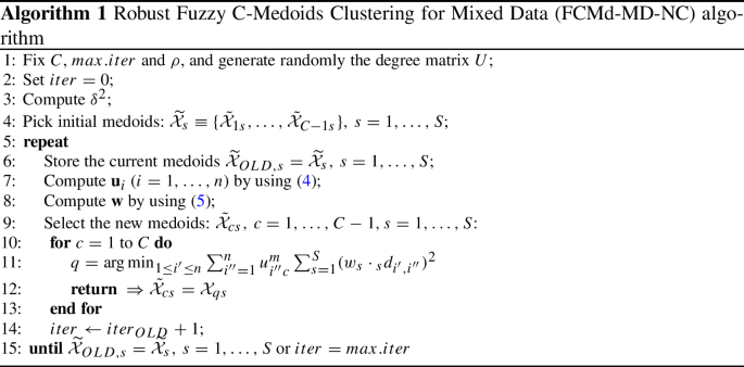
• 1. The fuzzy clustering algorithm that minimizes (3) is built by adopting an estimation strategy based on the Fu and Albus heuristic algorithm (Fu and Albus 1977). Indeed, the alternating optimization estimation procedure cannot be adopted because the necessary conditions cannot be derived by differentiating the objective function in (3) with respect to the medoids. The fuzzy clustering procedure is illustrated in Algorithm 1.

  

• 2. The computational complexity of the algorithm is due to three components: (i) the computation of the S dissimilarity matrices for each attribute type; (ii) the exhaustive search for the medoids; (iii) the computation of the attribute weights. While it is difficult to deal with the latter issue, it is possible to cope with the former two. First, the PAM approach requires that the distance matrix is computed only once at the beginning of the clustering process, and not at each iteration, thus decreasing dramatically the computing time required. Secondly, the search for the optimal medoids can be accelerated by “linearising” the clustering process, as in Krishnapuram et al. (2001), so that the complexity is linear in the number of units.

• 3. The degree of fuzziness of the resulting clusters is determined by m. The parameter can be pre-estimated by considering the usual fuzzy cluster-validity indices (see D’Urso and Maharaj 2009). However, since the medoid always has a membership of one in the cluster, raising its membership to the power of m has no effect on the medoid, while all other memberships decrease to 0. Thus, when m is high, the mobility of the medoids from iteration to iteration may be lost. For this reason, a value of m between 1 and 1.5 is recommended (Krishnapuram et al. 2001).

Remark 2

(Distances and dissimilarities)

One crucial decision in the clustering process for mixed data is the choice of suitable distance, or dissimilarity, measure for each attribute type. The choice is mainly heuristic, based on the data at hand and on the peculiar properties of each distance measure.

An admittedly non-exhaustive list of possible distance measures for several attribute types is reported in Table 2 (D’Urso and Massari 2019).

It should be highlighted that any kind of dissimilarity measure can be used in the proposed method. As in the standard non-hierarchical clustering algorithm e.g., k-means, k- medoids, the choice of the distance measure adopted in the clustering procedure is exogenous, so in the proposed method the choice of the distance measures for each attribute types is fixed beforehand. Any subset of variables can be managed with any of the dissimilarity measures presented in Table 2, and contribute to the “mixed” distance matrix in (2).

Table 2 Some distance measures and dissimilarity indices for different attribute types (integration of D’Urso and Massari (2019))

Remark 3

(Weighting system) The weights of the different attribute types in the clustering process are objectively provided by the model as shown in (5) and in the Appendix. An attribute type which displays a good separation into different groups should play a more significant role in clustering of data objects, against all other attribute types (Yeung and Wang 2002; Ahmad and Dey 2007). Indeed, the weight $w_s$ measures the within clusters similarity for the variables of the s-th type. Thus, the optimization procedure gives more relevance to the variable types capable to increase the within cluster similarity among the units.

Remark 4

(Determining the optimal number of clusters) A widely used cluster validity criterion for selecting C is the Xie-Beni criterion (Xie and Beni 1991), which can be suitably adapted for FCMd-MD-NC as follows:

$$\begin{aligned} \min _{C \in \Omega _C}:\, I_{XB}=\frac{\sum _{i=1}^{n}\sum _{c=1}^{C}u_{ic}^{m}d({\mathcal {X}}_i,\tilde{{\mathcal {X}}}_c)}{n\cdot \min _{c,c'}d(\tilde{{\mathcal {X}}}_c,\tilde{{\mathcal {X}}}_{c'})}= \frac{J}{n\cdot \min _{c,c'}d(\tilde{{\mathcal {X}}}_c,\tilde{{\mathcal {X}}}_{c'})}, \end{aligned}$$

(7)

where $\Omega _C$ represents the set of possible values of $C\,(C<n)$, and d(.) is the overall weighted distance (2).

The numerator of $I_{XB}$ represents the total within-cluster distance. The ratio J/n measures the compactness of the fuzzy partition. The smaller this ratio, the more compact a partition with a given number of clusters. The minimum distance between centroids at the denominator of $I_{XB}$ is a measure of the separation between clusters. The greater this distance, the more separate a data partition with a given number of clusters. Therefore, letting the number of clusters vary over the set $\Omega _C$, the optimal number of clusters is identified in correspondence with the lower value of $I_{XB}$.

2.2 Fuzzy profiling of the clusters

Results of cluster analysis can be summarized in the profiling phase where internal and external variables—i.e., variables involved and not involved in the cluster algorithm, respectively—are used to characterise and interpret the clusters (Everitt et al. 2011; Hair et al. 1998). In the case of fuzzy clustering algorithms, the $(n\times C)$ membership degrees matrix ${\mathbf {U}}=\{u_{ic}:\,i=1,\ldots ,n,\,c=1,\ldots ,C\}$ can be used to properly weigh the observations on profiling variables and further describe the final clusters (D’Urso et al. 2013, 2016).

Let $X=\{x_1,\ldots ,x_n\}$ be a quantitative variable observed on the sample. The weighted average of X in the c-th cluster is:

$$\begin{aligned} \mu _{X_c}=\frac{\sum _{i=1}^{n}u_{ic}x_i}{\sum _{i=1}^{n}u_{ic}}. \end{aligned}$$

(8)

As it can be seen, the greater is the membership degree of unit i to cluster c, the greater is the contribution of observation $x_i$ to the weighted average.

Similarly, let $Y=\{y_1,\ldots ,y_n\}$ be a categorical variable with $L\;(L\ge 2)$ categories. Let l be the generic category, and $y_{il}$ the observation in the i-th unit, which is equal to 1 if the category is observed on the i-th unit and 0 otherwise. The weighted proportion of the l-th category in the c-th cluster is:

$$\begin{aligned} w_{Y_{lc}}=\frac{\sum _{i=1}^{n}y_{il}u_{ic}}{\sum _{i=1}^{n}u_{ic}}. \end{aligned}$$

(9)

The concept of weighted averages and weighted proportions can be easily extended to other attribute types.

3 Simulation study

The aim of this simulation study is to highlight the capability of the FCMd-MD-NC model of correctly clustering objects in the presence of outliers. To this aim two distance matrices related to two groups of variables were generated, and outliers were added.

A dataset of $n=90$ objects was simulated, with two numeric continuous variables, $X_1,\,X_2$ and three numeric discrete variables, $X_3,\, X_4,\, X_5$ ($S=2$). In particular, $X_1$ and $X_2$ are both generated from the Uniform distribution. (Different numbers of objects were considered with similar results). $X_3$, $X_4$ and $X_5$ are discrete variables, with two, three and four values, respectively. Then, the set of variables is:

$$\begin{aligned}&{\mathcal {X}}=\{X_1,\,X_2\,X_3,\,X_4,\,X_5\}=\{{\mathcal {X}}_1,\,{\mathcal {X}}_2\}\\&\text {where}\\&{\mathcal {X}}_1=\{X_1,\,X_2\},\qquad {\mathcal {X}}_2=\{X_3,\,X_4,\,X_5\}. \end{aligned}$$

Objects are grouped into three well separated and equal sized clusters according to both continuous and discrete variables.

The three clusters were obtained as follows (Figs. 1, 2):

• cluster 1: $X_1$ and $X_2$ with Uniform density in the intervals [0;1],[2;3]; $X_3,\, X_4,\, X_5$ in the sets {1,2}, {1,2,3}, {1,2,3,4} with probability distributions {0.96,0.04}; {0.03, 0.94, 0.03}; {0.03, 0.94, 0.03, 0.00};

• cluster 2: $X_1$ and $X_2$ with Uniform density in the intervals [1;2],[0;1]; $X_3,\, X_4,\, X_5$ in the sets {1,2}, {1,2,3}, {1,2,3,4} with probability distributions {0.04,0.96}; {0.94, 0.03, 0.03}; {0.00, 0.03, 0.94, 0.03};

• cluster 3: $X_1$ and $X_2$ with Uniform density in the intervals [2;3],[1;2]; $X_3,\, X_4,\, X_5$ in the sets {1,2}, {1,2,3}, {1,2,3,4} with probability distributions {0.04,0.96}; {0.03, 0.03, 0.94}; {0.00, 0.03, 0.03, 0.94}

A number of outliers equal to 6 ($6.{\bar{6}}$%) and 12 ($13.{\bar{3}}$%) was generated. Different simulation scenarios have been considered:

• 1. outliers for the continuous and the discrete variables;

• 2. outliers for the two continuous variables;

• 3. outliers for the three discrete variables.

The outliers of the continuous variables were generated according to Normal distributions; of the discrete variables according to discrete distributions. The euclidean distance was used to generate the two distance matrices related to the two groups of variables.

Fig. 1

Simulated data—numerical variables of the three clusters without (left) and with (right) outliers

Fig. 2

Simulated data—numerical discrete variables of the three clusters without (top) and with (bottom) outliers

We expected that, given the weighting structure, FMDd-MD-NC should be able to correctly classify the objects, despite the presence of outliers.

The correctness of clustering is evaluated by means of the Fuzzy Rand Index (FRI) to compare the obtained fuzzy partition with the reference crisp partition (30 objects in each cluster).

The simulation study involved 100 replications (different numbers of replications were considered with similar results). Two values of the fuzziness parameter m were considered, 1.3 and 1.5. For each replication the weights computed for the two attributes and the FRI were collected. The results are reported in Table 3.

As for the correctness of the clustering, FCMd-MD-NC shows the expected robustness to outliers. Values of FRI are well above 0.90 in all scenarios and in all replications, thus indicating that the obtained fuzzy partitions are very close to the theoretical cluster partition. As for the attribute type weights, the two attribute types are weighted as expected according to their clustering structure. In all 100 replications FCMd-MD-NC attributed approximately equal weights to the two attributes in Scenario 1, greater weight to the continuous variables in Scenario 2 as the outliers of the numerical variables are assigned to the noise cluster, greater weight to the discrete variables in Scenario 3, as the outliers of the discrete variables are assigned to the noise cluster.

For comparative assessment the simulations have been run without the presence of the noise cluster. As it can be seen from Table 3, the results obtained with the model FCMd-MD-NC outperform the results obtained with the Fuzzy C-Medoids Clustering for Mixed Data (FCMd-MD) model. In all 100 replications FCMd-MD attributed approximately equal weights to the two attributes in Scenario 1, greater weight to the discrete variables in Scenario 2 as the outliers of the continuous variables are not assigned to the noise cluster, greater weight to the continuous variables in Scenario 3, as the outliers of the discrete variables are not assigned to the noise cluster.

The flipped behaviour of the two models in weighting the two distance matrices - of the continuos variables and of the discrete variables - deserves a comment. In the model FMDd-MD without noise cluster the outliers are assigned to the three clusters with great membership, and according to (20) they contribute to a great distance of the objects from the medoids; in the model FCMd-MD-NC with noise cluster the outliers are assigned to the three clusters with small membership being assigned to the noise cluster, and according to (20) they contribute to a small distance of the objects from the medoids, resulting in a greater weight.

4 Application: clustering of football players

The aim of this application is the clustering of football players based on attributes of different types. Professional football clubs invest a lot of resources in the recruitment of players. The clustering of football players based on performance data may be useful for prototyping successful players and for providing insights to football managers when assessing players.

Data for this application are drawn from whoscored.¹ The units are the players that have played in the “Serie A” tournement at least 200 min in the season 2018/19. The choice of 200 min follows from the choice of evaluating performances (goal, shots) per game (90 min). Less than 200 min would have led to re-proportioning the number of goals of a player, who scored a goal having played only 10 min, at 9 per game. The considered players were 397 from the initial number of 544. The teams of the season were: AC Milan, Atalanta, Bologna, Cagliari, Chievo, Empoli, Fiorentina, Frosinone, Genoa, Inter, Juventus, Lazio, Napoli, Parma Calcio 1913, Roma, Sampdoria, Sassuolo, SPAL 2013, Torino, Udinese. The most represented (greater than 3.0%) nationalities were Italy (39.3%), Argentina (6.3%), Brazil (5.8%), France (3.5%), Spain and Croatia (3.0%).

The considered variables are “Performance variables”, “Success Variables” and “Position variables”. The variables are grouped into four groups ($S=4$) as described in Table 4 according to their type and meaning (Akhanli and Hennig 2017), in order to use an appropriate distance for each type and to obtain endogeneously the weight of each group in the definition of the clusters.

Table 3 Simulation study

Performance (Upper level) variables are all count variables and can be grouped into three categories in terms of their meaning: Defensive (Tackles, Blocks); Offensive (Shots, Goals, Aerials, Dribbles); Pass (Passes, Keypasses). Some performance variables are partitioned into different sub-parts (Lower level variables). The sub-parts of Shots are body parts (four categories head, left foot, right foot, other), situations (four categories counter, open play, penalty taken, setpiece), zones (three categories out of box, penalty area, six yard box), accuracy; the sub-parts of Goals are body parts, situations, zones. The Success variables evaluate the success rates of shot and goal upper level count variables. The position variables are eleven: Attack, Defensive and Milfielder each of which either in the Centre, Left or Right side; Forward and Defensive Milfielder. They are binary variables. Since a player can play in several positions, multiple binary variables are considered. The position variables are represented in Fig. 3. The variables, available in the database whoscored, have been used in previous studies (Akhanli and Hennig 2017) The variables and their summary statistics are reported in Table 4; alongside with the weights computed in the clustering process for the different attributes types as in (5).

Table 4 Variables

Fig. 3

Position variables

4.1 Data preprocessing

The Performance Upper level variables are represented per 90 min. The histograms of the performance variables are presented in Fig. 4.

The Success variables are represented as percentages. The Success Upper level variables Assists, Passes Aerials and Dribbles are percentages of accurate/successful actions over the total number of actions.

The Success Lower level compositions of Goals by body parts, situations and zones are percentages of success over the number of shots in the related sub-part (goal body part head over shots body part head).

The sub-parts of the Performance Upper level variable are transformed into percentages. If a player has scored 10 Goals per 90 min, of which 3 in situation out of box, 5 penalty area and 2 six yard box, the compound variables offensive Goals zones shows the values (30%, 50%, 20%) in the categories out of box, penalty area, six yard box.

The eleven position variables are binary variables.

The Performance Upper level count variables are standardised by average absolute deviation, whereas lower level compositions are standardised by the pooled average absolute deviation from all categories belonging to the same composition of lower level variables.

The Manhattan distance has been used for the Performance Upper level variables and for the Success Upper/Lower level variables.

The Performance Lower level variables are compositional data in the sense of Aitchison (Aitchison 1986), who set up an axiomatic theory for the analysis of compositional data. According to Akhanli and Hennig (2017), for the compositional percentage data the simple Manhattan distance is used as more appropriate.

The distance measure used for the Position variables has been proposed in Hennig and Hausdorf (2006) and incorporates geographic distances. The proposed “geco” (“geographic distance and congruence”) coefficient considers both the number of positions (geographic locations) shared by two players and the geographic relations of the occupied positions. Let $A_1, A_2 \subseteq R$ be the vectors of positions (presence-absence) of players a and b in the eleven positions of the football field (Fig. 3). Assume that there is a distance $d_R$ defined on R; $d_R$ is the geographic distance between positions (geographic locations) (euclidean distance in Table 5). For example, assuming segments of length 1 between adjacent positions on the same line, the geographic distance between positions DMC and MR is $\sqrt{(1^2+1^2)}=\sqrt{2}$; between positions DMC and AMR $\sqrt{(2^2+1^2)}=\sqrt{5}$ . The “geco” distance between players a in region $A_1$ and player b in region $A_2$ is defined as :

$$\begin{aligned} d_G(A_1,A_2)=\frac{1}{2}\left( \frac{\sum _{a \in A_1}\underset{b \in A_2}{\text {min}}d_R(a,b)}{|A_1|}+\frac{\sum _{b \in A_2}\underset{a \in A_1}{\text {min}}d_R(a,b)}{|A_2|}\right) \end{aligned}$$

(10)

where and $A_i$ denotes the number of elements in the geographical region of the $i-th$ object. Then, $d_G$ is the mean of the average geographic distance of all units of $A_1$ to the respective closest unit in $A_2$ and the average geographic distance of all units of $A_2$ to the respective closest unit in $A_1$. From the definitions it follows $d_G(A, A)=0$, $d_G(A,B)>0$, $d_G(A,B)=d_G(B,A)$.

Table 5 Distances between position variables

Fig. 4

Histograms of the performance variables

4.2 Results

Different values of the fuzziness parameter m ($m=1.3, 1.5, 2.0$) and of the number of clusters C ($C=3, 4, 5, 6)$ have been considered. According to the Xie-Beni criterion, the optimal number of clusters is three, with a value of $m=1.3$. The numerosity of the clusters is 109, 127, 112, 49 (noise cluster). The medoids of the three clusters are players 278, 288 and 91. The attributes’ weights obtained during the optimization process are reported in the last column of Table 4. The Performance variables and the Success variables provide the greatest contribution to the clustering process.

Reported in Table 6 are the three medoids’ characteristics, separately for each attribute type (a subset for the Success Upper level variables). The numeric Lower level compositional variables are not presented due to the small weight assigned in the clustering procedure.

Table 6 Medoids’ characteristics -football data

The first cluster is represented by a player showing a discrete number of actions (Performance Upper level), successful (Goal/Shots, Assists accuracy, Aerials won and Dribbles successful) (Success Upper/Lower level).

The second cluster is represented by a player showing a limited number of actions (Performance Upper level), unsuccessful (Goal/Shots=0.0) (Success Upper/Lower level).

The third cluster is represented by a player showing a high number of actions per 90 min (Performance Upper level), very successful (Goal/Shots, Passes accuracy, and Dribbles successful) (Success Upper/Lower level).

The three clusters are similar with respect to the positions of the players. It is worth noting that the medoid players in cluster 1 and 3 have played in the Forward position. We observe that the player Ronaldo, who shows one of the highest values of Goal/Shots, is assigned to the third cluster.

As expected, the noise cluster shows heterogeneity of players with respect to the variables, as expected (otherwise there would be one more cluster).

In Figs. 5, 6, 7, and 8 the composition of the clusters with respect to some of the segmentation variables is reported. Percentages are calculated taking into account the membership degrees to each cluster, as explained in Sect. 2.2. The composition of the clusters is consistent with the three medoids.

We observe in Fig. 5 the prevalence of Goals in cluster 3.

We observe in Fig. 6 that in the first cluster the successful percentage of shots that gives rise to a goal is played with body part left foot, situation setpiece and zone six yard box; in the second cluster with body part right foot, situation setpiece and zone six yard box; in the third cluster with body part right foot, situation open play and zone six yard box.

We observe in Fig. 7 that in the three clusters the greater percentage of Goals is played in the category of body part right foot, in situation open play and in zone penalty area; similarly for the Shots.

We observe in Fig. 8 the prevalent positions played in the three clusters.

Fig. 5

Performance variables weighted with memberships within clusters. Cluster 1, 2, 3 top to bottom

Fig. 6

Success variables weighted with memberships within clusters. Cluster 1, 2, 3 top to bottom

Fig. 7

Compositional variables weighted with memberships within clusters. Cluster 1, 2, 3 top to bottom

Fig. 8

Position variables weighted with memberships within clusters. Cluster 1, 2, 3 top to bottom

Figure 9 report a ternary plot with the membership degrees obtained with FCMd-MD-NC, for the three clusters. While there are several players that are fuzzy assigned, in particular to the first and the third cluster, over 50% of the units are allocated to a single cluster with a membership degree above 0.70.

Fig. 9

Ternary plot for the membership degrees obtained with FCMd-MD-NC applied to football data

5 Discussion and final remarks

In this paper, following the Partitioning Around Medoids (PAM) approach, we propose a robust fuzzy clustering with noise cluster and weighting system for mixed attributes. A simulation study is proposed. The model is used for analysing massive dataset in sport, i.e. for clustering football players based on their performance and positional attributes.

The clustering model allows different types of variables, or attributes, to be taken into account. A weight is objectively assigned to the distance matrix associated to each set of attributes during the optimization process. The weights reflect the the relevance of each attribute type in the clustering results. A noise cluster neutralizes the effect of outliers. The simulation study has shown the ability of the model to weight properly the distance matrices of the attributes in the presence of outliers. The application to the clustering of football players on the basis of distance matrices of different attributes has shown the need to manage separately mixed type data. The obtained weights allow to understand which is the most relevant set of attributes in partitiong the players. The model applied to the profiling of players provides insights on the characteristics of successful players.

The proposed clustering model has targeted some relevant issues in the research field. A mixed distance for the different attributes is considered; weights to distances related to different attribute types giving relevance to the variable types capable to increase the within cluster similarity are objectively provided by the model; a noise cluster represented by a noise prototype is introduced to achieve robustness with respect to outliers. For the practictioners, clustering of football players on the basis of playing characteristics, position, performance and success variables is relevant for clubs, either to drive team formation and selection of players, or for determining the value of a football player in the transfer window period (Behravan and Razavi 2021; Shelly et al. 2020; Narizuka and Yamazaki 2019). In football, performance assessment has typically been conducted to predict player’s abilities, to rate player’s performances, to drive their physical training or to explain a team’s success (Mohr et al. 2003; Di Salvo et al. 2007; McHale et al. 2012).

Future work will deal with other robust clustering solutions, the inclusion of financial variables of the player and of the team, the temporal aspect of the playing variables, if available, the interactions among team members and with the opposing players in the course of a game.

Appendix

In the following, we prove the iterative solutions (4)–(5).

Proof

First, fixed $w_s$, we determine the membership degrees $u_{ic}$. We consider the Lagrangian function analyzing the objective function not splitted into $C-1$ clusters and the noise cluster:

$$\begin{aligned} L_m({\mathbf {u}}_i,\lambda )=\sum _{i=1}^{n}\sum _{c=1}^{C}u_{ic}^md_{ic}^2-\lambda \left( \sum _{c=1}^{C}u_{ic}-1\right) \end{aligned}$$

(11)

where ${\mathbf {u}}_i=(u_{i1},\ldots ,u_{ic},\ldots ,u_{iC})^{\prime }$ and $\lambda$ is the Lagrange multiplier. Therefore, we set the first derivatives of (11) with respect to $u_{ic}$ and $\lambda$ equal to zero, yielding:

$$\begin{aligned} \frac{\partial L_m({\mathbf {u}}_i,\lambda )}{\partial u_{ic}}=0 \,&\Leftrightarrow \, mu_{ic}^{m-1}d_{ic}^2-\lambda =0 \end{aligned}$$

(12)

$$\begin{aligned} \frac{\partial L_m({\mathbf {u}}_i,\lambda )}{\partial \lambda }=0\,&\Leftrightarrow \, \sum _{c=1}^{C}u_{ic}-1=0 \end{aligned}$$

(13)

From (12) we obtain:

$$\begin{aligned} u_{ic}=\left( \frac{\lambda }{m}\frac{1}{d_{ic}^2}\right) ^{\frac{1}{m-1}} \end{aligned}$$

(14)

and, by considering (13):

$$\begin{aligned} \frac{\lambda }{m}^{\frac{1}{m-1}}=\frac{1}{\left( \frac{1}{\sum _{c=1}^{C}d_{ic}^2}\right) ^{\frac{1}{m-1}}}. \end{aligned}$$

(15)

Finally, substituting (15) in (14) and taking into account the decomposition into the $C-1$ clusters and the noise cluster we obtain $u_{ic}$ as in (4).

Then, fixed $u_{ic}$ we derive $w_s$. The Lagrangian function is:

$$\begin{aligned} L_m({\mathbf {w}},\xi )=\sum _{i=1}^{n}\sum _{c=1}^{C-1}u_{ic}^m\sum _{s=1}^{S}(w_s \cdot {}_sd_{ic})^2+\sum _{i=1}^{n}u_{iC}^m\delta ^2-\xi \left( \sum _{s=1}^{S}(w_s-1)\right) \end{aligned}$$

(16)

where ${\mathbf {w}}=(w_1,\ldots ,w_s,\ldots ,w_S)^{\prime }$ and $\xi$ is the Lagrange multiplier. By setting the first derivatives of (16) with respect to $w_s$ and $\xi$ equal to zero, we obtain respectively:

$$\begin{aligned} \frac{\partial L_m({\mathbf {w}},\xi )}{\partial w_s}=0\,&\Leftrightarrow \, 2w_s\sum _{i=1}^{n}\sum _{c=1}^{C-1}u_{ic}^m \cdot {}_sd_{ic}^2-\xi =0 \end{aligned}$$

(17)

$$\begin{aligned} \frac{\partial L_m({\mathbf {w}},\xi )}{\partial \xi }=0\,&\Leftrightarrow \, \sum _{s=1}^{S}w_s-1=0. \end{aligned}$$

(18)

From (17) we have:

$$\begin{aligned} w_s=\frac{\xi }{2\sum _{i=1}^{n}\sum _{c=1}^{C-1}u_{ic}^m \cdot {}_sd_{ic}^2} \end{aligned}$$

(19)

and using (18):

$$\begin{aligned} \frac{\xi }{2}=\frac{1}{\sum _{s=1}^{S}\left( \frac{1}{\sum _{i=1}^{n}\sum _{c=1}^{C-1}u_{ic}^m \cdot {}_sd_{ic}^2}\right) }. \end{aligned}$$

(20)

Then, replacing (20) in (19), we obtain $w_s$, as in (5). $\square$

References

Adhikari, A., Majumdar, A., Gupta, G., & Bisi, A. (2020). An innovative super-efficiency data envelopment analysis, semi-variance, and shannon-entropy-based methodology for player selection: evidence from cricket. Annals of Operations Research, 284(1), 1–32.
Ahmad, A., & Dey, L. (2007). A k-mean clustering algorithm for mixed numeric and categorical data. Data & Knowledge Engineering, 63(2), 503–527.
Aitchison, J. (1986). The statistical analysis of compositional data. Chapman & Hall, Ltd.
Akhanli, S. E., & Hennig, C. (2017). Some issues in distance construction for football players performance data. Archives of Data Science, Series A (Online First), 2(1):17 S. online.
Andrienko, G., Andrienko, N., Budziak, G., Dykes, J., Fuchs, G., Landesberger, T., & Weber, H. (2017). Visual analysis of pressure in football. Data Mining and Knowledge Discovery, 31, 1–47.
Behravan, I., & Razavi, S. M. (2021). A novel machine learning method for estimating football playersâ value in the transfer market. Soft Computing, 25, 2499–2511.
Berndt, D. J. & Clifford, J. (1994). Using dynamic time warping to find patterns in time series. In Proceedings of the AAAI-94 Workshop Knowledge Discovery in Databases, pages 359–370. Seattle, WA.
Carpita, M., Ciavolino, E., & Pasca, P. (2019). Exploring and modelling team performances of the Kaggle European soccer database. Statistical Modelling, 19(1), 74–101.
Cea, S., Durán, G., Guajardo, M., Sauré, D., Siebert, J., & Zamorano, G. (2020). An analytics approach to the FIFA ranking procedure and the World Cup final draw. Annals of Operations Research, 286(1), 119–146.
Corduas, M., & Piccolo, D. (2008). Time series clustering and classification by the autoregressive metric. Computational Statistics & Data Analysis, 52(4), 1860–1872.
Dadeliene, R., Dadelo, S., Pozniak, N., & Sakalauskas, L. (2020). Analysis of top kayakersâ training-intensity distribution and physiological adaptation based on structural modelling. Annals of Operations Research, 289(2), 195–210.
Davé, R. N. (1991). Characterization and detection of noise in clustering. Pattern Recognition Letters, 12, 657–664.
Dawson, P., Dobson, S., Goddard, J., & Wilson, J. (2007). Are football referees really biased and inconsistent?: Evidence on the incidence of disciplinary sanction in the English premier league. Journal of the Royal Statistical Society: Series A - Statistics in Society, 170(1), 231–50.
Di Salvo, V., Baron, R., Tschan, H., Montero, F., Bachl, N., & Pigozzi, F. (2007). Performance characteristics according to playing position in elite soccer. International Journal of Sports Medicine, 28, 222–7.
D’Urso, P., De Giovanni, L., Disegna, M., & Massari, R. (2013). Bagged clustering and its application to tourism market segmentation. Expert Systems with Applications, 40(12), 4944–4956.
D’Urso, P., Disegna, M., Massari, R., & Osti, L. (2016). Fuzzy segmentation of postmodern tourists. Tourism Management, 55, 297–308.
D’Urso, P., & Giordani, P. (2004). A least squares approach to principal component analysis for interval valued data. Chemometrics and Intelligent Laboratory Systems, 70(2), 179–192.
D’Urso, P., & Giordani, P. (2006). A weighted fuzzy c-means clustering model for fuzzy data. Computational Statistics & Data Analysis, 50(6), 1496–1523.
D’Urso, P., & Maharaj, E. (2009). Autocorrelation-based fuzzy clustering of time series. Fuzzy Sets and Systems, 160(24), 3565–3589.
D’Urso, P., & Massari, R. (2013). Fuzzy clustering of human activity patterns. Fuzzy Sets and Systems, 215, 29–54.
D’Urso, P., & Massari, R. (2019). Fuzzy clustering of mixed data. Information Sciences, 505, 513–534.
Eskin, E., Arnold, A., Prerau, M., Portnoy, L., and Stolfo, S. (2002). A geometric framework for unsupervised anomaly detection. In Applications of data mining in computer security, pp. 77–101. Springer.
Everitt, B., Landau, S., Leese, M., and Stahl, D. (2011). Cluster analysis. Wiley, Ltd, London, 5th edition.
Everitt, B. S. (1988). A finite mixture model for the clustering of mixed-mode data. Statistics & Probability Letters, 6(5), 305–309.
Fortuna, F., Maturo, F., & Battista, T. (2018). Clustering functional data streams: Unsupervised classification of soccer top players based on google trends. Quality and Reliability Engineering, 34, 1448–1460.
Fu, K., & Albus, J. (1977). Syntactic pattern recognition. Springer.
Galariotis, E., Germain, C., & Zopounidis, C. (2018). A combined methodology for the concurrent evaluation of the business, financial and sports performance of football clubs: The case of France. Annals of Operations Research, 266(1), 589–612.
Gates, K. M., Lane, S. T., Varangis, E., Giovanello, K., & Guiskewicz, K. (2017). Unsupervised classification during time-series model building. Multivariate Behavioral Research, 52(2), 129–148.
Geenens, G., & Cuddihy, T. (2018). Nonâparametric evidence of secondâleg home advantage in European football. Journal of the Royal Statistical Society Series A, 181(4), 1009–1031.
Goes, F., Kempe, M., Meerhoff, R., & Lemmink, K. A. (2018). Not every pass can be an assist: A data-driven model to measure pass effectiveness in professional soccer matches. Big Data, 7, 57–70.
Goossens, D., Beliën, J., & Spieksma, F. (2012). Comparing league formats with respect to match importance in Belgian football. Annals OR, 194, 223–240.
Gowda, K. C. & Diday, E. (1991). Symbolic clustering using a new dissimilarity measure. Pattern Recognition, 24(6), 567–578.
Groll, A., Manisera, M., Schauberger, G., & Zuccolotto, P. (2018). Guest editorial statistical modelling for sports analytics. Statistical Modelling, 18(5–6), 385–387.
Hair, J. F., Anderson, R. E., Tatham, R. L., and Black, W. C. (1998). Multivariate data analysis. Upper Saddle River.
Hamming, R. (1950). Error detecting and error correcting codes. Bell System Technical Journal, 29(2), 147–160.
Hennig, C., & Hausdorf, B. (2006). A robust distance coefficient between distribution areas incorporating geographic distances. Systematic Biology, 55(1), 170–175.
Karney, C. F. (2013). Algorithms for geodesics. Journal of Geodesy, 87(1), 43–55.
Koopman, S. J., & Lit, R. (2015). A dynamic bivariate poisson model for analysing and forecasting match results in the English premier league. Journal of the Royal Statistical Society Series A, 178(1), 167–186.
Krishnapuram, R., Joshi, A., Nasraoui, O., & Yi, L. (2001). Low-complexity fuzzy relational clustering algorithms for web mining. IEEE Transactions on Fuzzy Systems, 9(4), 595–607.
Kruskal, J. (1983). An overview of sequence comparison. In D. Sankoff & J. Kruskal (Eds.), Time warps, string edits, and macromolecules: The theory and practice of sequence comparison (pp. 1–44). Reading, MA: Addison-Wesley Publishing Company.
Levenshtein, V. (1966). Binary codes capable of correcting deletions, insertions and reversals. Soviet Physics Doklady, 10, 707–710.
Lu, H., & Tan Y. P. (2003). Unsupervised clustering of dominant scenes in sports video. Pattern recognition Letters, 24(15), 2651–2662.
Maharaj, E. A., D’Urso, P., & Galagedera, D. U. (2010). Wavelet-based fuzzy clustering of time series. Journal of Classification, 27(2), 231–275.
McHale, I. G., & Relton, S. D. (2018). Identifying key players in soccer teams using network analysis and pass difficulty. European Journal of Operational Research, 268(1), 339–347.
McHale, I. G., Scarf, P. A., & Folker, D. E. (2012). On the development of a soccer player performance rating system for the English premier league. Interfaces, 42, 339–351.
Metulini, R., Manisera, M., & Zuccolotto, P. (2018). Modelling the dynamic pattern of surface area in basketball and its effects on team performance. Journal of Quantitative Analysis in Sports, 14(3), 117–130.
Mohr, M., Krustrup, P., & Bangsbo, J. (2003). Match performance of high-standard soccer players with special reference to development of fatigue. Journal of Sports Sciences, 21, 519–528.
Narizuka, T., & Yamazaki, Y. (2019). Clustering algorithm for formations in football games. Scientific Reports, 9.
Narizuka, T. and Yamazaki, Y. (2020). Clarifying the structure of serious head and spine injury in youth rugby union players. PLOS ONE, 15(7).
Nikolaidis, Y. (2015). Building a basketball game strategy through statistical analysis of data. Annals of Operations Research, 227(1), 137–159.
Palacios-Huerta, I. (2004). Structural changes during a century of the worldâs most popular sport. Statistical Models & Applications, 13, 241–258.
Shelly, Z., Reuben F. Burch V, W. T., Strawderman, L., Piroli, A., and Bichey, C. (2020). Using k-means clustering to create training groups for elite american football student-athletes based on game demands. International Journal of Kinesiology & Sports Science, 8(2), 47–63.
Sokal, R. R. (1958). A statistical method for evaluating systematic relationship. University of Kansas Science Bulletin, 28, 1409–1438.
Ulas, E. (2021). Examination of national basketball association (nba) team values based on dynamic linear mixed models. PLOS ONE, 16(6), 1–16.
Van Bulck, D., Goossens, D., and Spieksma, F. (2019). Scheduling a non-professional indoor football league: A tabu search based approach. Annals of Operations Research, 275.
Xie, X. L., & Beni, G. (1991). A validity measure for fuzzy clustering. IEEE Transactions on Pattern Analysis and Machine Intelligence, 13(8), 841–847.
Yang, C.-H., Lin, H.-Y., & Chen, C.-P. (2014). Measuring the efficiency of nba teams: Additive efficiency decomposition in two-stage dea. Annals of Operations Research, 217(1), 565–589.
Yang, M., & Ko, C. (1996). On a class of fuzzy \(c\)-numbers clustering procedures for fuzzy data. Fuzzy Sets and Systems, 84(1), 49–60.
Yeung, D. S., & Wang, X. (2002). Improving performance of similarity-based clustering by feature weight learning. IEEE Transactions on Pattern Analysis and Machine Intelligence, 24(4), 556–561.
Zuccolotto, P., Manisera, M., & Sandri, M. (2018). Big data analytics for modeling scoring probability in basketball: The effect of shooting under high-pressure conditions. International Journal of Sports Science and Coaching, 13(4), 569–589.
Author information
Authors and Affiliations
Corresponding author
Additional information
Publisher's Note
Springer Nature remains neutral with regard to jurisdictional claims in published maps and institutional affiliations.