
Abstract
The EUREF Permanent Network Densification is a collaborative effort of 26 European GNSS analysis centers providing series of daily or weekly station position estimates of dense national and regional GNSS networks, in order to combine them into one homogenized set of station positions and velocities. During the combination, the station meta-data, including station names, DOMES numbers, and position offset definitions were carefully homogenized, position outliers were efficiently eliminated, and the results were cross-checked for any remaining inconsistencies. The results cover the period from March 1999 to January 2017 (GPS week 1000-1933) and include 31 networks with positions and velocities for 3192 stations, well covering Europe. The positions and velocities are expressed in ITRF2014 and ETRF2014 reference frames based on the Minimum Constraint approach using a selected set of ITRF2014 reference stations. The position alignment with the ITRF2014 is at the level of 1.5, 1.2, and 3.2 mm RMS for the East, North, Up components, respectively, while the velocity RMS values are 0.17, 0.14, and 0.38 mm/year for the East, North, and Up components, respectively. The high quality of the combined solution is also reflected by the 1.1, 1.1, and 3.5 mm weighted RMS values for the East, North, and Up components, respectively.
Introduction and history
The campaign-style and continuously operating GNSS reference station (CORS) networks are the main interdisciplinary tools of modern earth sciences exploited for reference frame maintenance, geokinematics, ionospheric studies or meteorology. At the beginning of the GPS era, the geodetic and geophysical approaches were slightly different: in geophysics, the GPS networks (mostly epoch/campaign solutions) concentrated on regions of tectonic interest and focused on the estimation of relative displacements, which are less sensitive to reference frame alignment. In geodesy, the primary target is always reference frame realization and maintenance from global to national scales implementing homogeneous products and standards (Altamimi and Collilieux 2009; Bruyninx et al. 2012). The early, epoch-type GPS campaign networks have been gradually replaced by dense, multi-purpose, multi-scale CORS networks, which are now processed and analyzed using harmonized strategies and standards in both geodesy and geophysics. A recent example is the European Plate Observing System (EPOS) project (Jeffery and Bailo 2014), where geodesists and geophysicists are analyzing and exploiting together the same GNSS infrastructure.
The combination of independent regional or global GNSS solutions makes stand-alone solutions compatible and allows creating large-scale solutions for velocity and strain rate modeling. One of the first global-scale approaches was the UNAVCO-funded GPSVEL project, where velocity solutions in SINEX format (IERS Message 103 2006) from all available sources were proposed to compile and deliver a homogenized velocity field estimate. On the global level, the International Association of Geodesy (IAG) Working Groups on “Regional Dense Velocity Fields” (2007–2011) (Bruyninx et al. 2013) and “Integration of Dense Velocity Fields in the ITRF” (2011–2015) (Legrand et al. 2014) first attempted to create a dense global velocity field by combining multi-year GNSS position/velocity solutions with full variance–covariance information, available in SINEX format from different continents. They concluded that, due to the inhomogeneity of meta-data handling and offset definitions in the different multi-year continental solutions, it was impossible to combine them reliably. Therefore, they changed strategy and started to combine the continental solutions first at the weekly level and then stack the weekly combined position solutions to derive multi-year position and velocity solutions.
In Europe, most countries operate dense CORS networks for serving their practical positioning and surveying needs. The GNSS data processing is often done at the national level with sophisticated software packages [e.g., BERNESE 5.2 (Dach et al. 2015), GAMIT (King and Bock 1996), GIPSY OASIS II (Zumberge et al. 1997)] using well-harmonized processing standards and parameters defined by IGS (https://kb.igs.org/hc/en-us/sections/200369273-Guiding-Documents), and extended by regional entities as EUREF (http://www.epncb.oma.be/_documentation/guidelines/guidelines_analysis_centres.pdf).
To take advantage of the available national processing results, the IAG sub-commission for Europe (EUREF) formed in 2015 the EPN Densification Working Group (http://euref.eu/TWG/WGdocs/WG_EPN_densification_charter.pdf). The Working Group is committed to collect and integrate the long-term national CORS network processing results delivered by EPN ACs. All ACs are following the well-defined EUREF processing standards, including the harmonized modeling of relevant environmental and technical parameters.
We present a review of the GNSS product combination approaches, discuss the rigorous long-term position combination technique in detail, and introduce the creation of a unique, unprecedented multi-year GNSS combination for Europe delivering a homogenized position and velocity solution incorporating most of the European CORS networks, which offered as reference for national and large-scale studies.
Combination approaches
The target of the combination of a set of position and/or velocity solutions is to derive an accumulated position and/or velocity field, where, in the optimal case, the combination homogenizes the input solutions and mitigates systematic errors of any of the individual contributions. Stations common to several solutions provide the option to tie these networks into a single and consistent position set and/or velocity field and also provide information on the relative systematic biases between the stand-alone solutions such as reference frame misalignment. Depending on the input data and the chosen mathematical tools, several combination approaches can be distinguished, which are briefly introduced and reviewed below.
Velocity-only combination
The simplest and easiest option is to combine pure 2D or UP velocities stemming from different sources, where the combination may be considered as
-
Velocity averaging This approach is unable to account for biases between the solutions and implicitly assumes that they are correctly expressed in the same reference frame. In a refined mode, the input solutions can also be weighted and the correlation matrices of the solutions are taken into account.
-
Rigid rotations around the auxiliary Euler-pole, where the model parameters are obtained by minimizing velocity differences at collocated sites (Hefty 2007). This method may significantly improve the reliability of the combination allowing the use of velocities expressed in a different or unknown reference frame. The method can also be used to detect internal inconsistent velocity subsets in a solution, which helps the better separation of the tectonic units (Savage 2018).
-
An inversion solving for translation and rotation rates which transforms all results into the desired common reference frame. This approach was implemented by Kreemer et al. (2014) for the realization of the Global Strain Rate Model, where the authors compiled > 15,000 velocities from 233 studies available in the literature and aligned them to the IGS08 reference frame. Additionally, they collected GPS data in RINEX format and performed a global-scale processing using the GIPSY OASIS II software deriving almost 7000 velocities.
The shortcomings of these approaches are:
-
The possible biases and the overall quality can only be checked and estimated at common stations,
-
No, or limited use of uncertainties and the variance–covariance matrix,
-
Loss of information on quality, because of the lack of direct access to position time series,
-
Possible site-specific biases caused by different processing standards.
Combination of multi-year position and velocity solutions
This approach combines independently created multi-year position and velocity solutions published in SINEX format with full variance–covariance information. Based on the mathematical handling of the input solution constraints, we may distinguish between the free network combination methodology proposed by Davies and Blewitt (2000), the direct combination of loosely constrained solutions (Devoti et al. 2017), and the combination based on the Minimum Constraint (MC) approach (Altamimi et al. 2002). The direct combination approach exploits the fact that no inversion problem exists for the generation of the solution variance–covariance matrix, and if only the velocity combination is concerned, the knowledge of the position estimates is not needed. The preferred option, however, is the MC approach, which was applied on global level by Legrand et al. (2014) in the IAG WG on “Integration of Dense Velocity Fields in the ITRF” and on regional scale by Nocquet and Calais (2003).
Although the combination of the multi-year stacked solutions minimizes the possible systematic errors related to the individual processing strategies and reliably connects the input solutions, it has similar critical issues as listed in the velocity level combination. An additional strong limiting factor is the need for the harmonized definition of the position discontinuity epochs due to equipment changes or any other local event causing position offsets or variation in the time series pattern. The combination can only work when the GNSS processing and station meta-data are fully harmonized before generating the multi-year solutions.
Large-scale processing of RINEX data
As shown by Kreemer et al. (2014), homogeneous position-velocity solutions can be derived through a global- or regional-scale processing of all available GNSS data. This approach guarantees by nature the homogeneity of the results, but also inherits several disadvantages:
-
It requires a huge effort from the analysis center in terms of data collection, cleaning, meta-data check and processing,
-
It may be limited by data access policies since not all RINEX data are necessarily freely available,
-
It lacks an independent check of processing strategy implementation, meta-data correctness, reference frame realization.
Those disadvantages may partially be eliminated if the large-scale data handling and processing is done in an organized way and several groups share the workload. The most recent example is the GNSS services in the frame of the EPOS infrastructure, where a central data node provides validated data/meta-data to, among others, two Pan-European Processing Centres [National Institute of Geophysics and Volcanology (INGV) in Italy and a consortium of University of Grenoble Alps and National Center for Scientific Research (UGA-CNRS) in France], which perform GIPSY OASIS II and GAMIT processing, respectively. They process practically the same network and their daily position SINEX solutions are checked and combined by a Combination Centre led by the first author of this paper. In addition, a dedicated center, located at the Royal Observatory of Belgium (ROB), is responsible for maintaining and validating up to date station meta-data (site logs). The established work-chain assures the optimal share of the workload, the elimination of occasional analysis center or data issues, and guarantees the long-term sustainability of the system. The only limiting factor is the need to access the GNSS RINEX data.
Multi-year combination of weekly pre-combined solutions
Several shortcomings of the previous approaches can be resolved if the combination is done not on the multi-year level, but starting with the weekly position solutions coming from different processing centers. An important advantage of this approach is that agencies which are not necessarily willing to share the RINEX data of their GNSS stations are more disposed to share the processing results of their data analysis. In these input data sets, first the meta-data inconsistencies including 4-character station identifier and DOMES numbers must be identified and cleaned, station naming and discontinuity definitions are harmonized, and outliers are removed. Then the individual weekly position files from all contributors are combined to create a series of combined weekly position SINEX files. These pre-combined files then enter into a multi-year combination to produce a cumulative position and velocity solution freed from, e.g., individual reference frame misalignment or inconsistent meta-data information.
Such an approach is routinely applied on the global level within the International GNSS Service (IGS), where the IGS Analysis Center Coordinator (ACC) tests the daily position SINEX inputs coming from the IGS Analysis Centers and creates a combined daily and weekly position SINEX series. The weekly solutions are then used for the regular update of the IGS multi-year product. On the regional level, such integration is also being done for North- and South America (Sánchez et al. 2015), and Europe (Bruyninx et al. 2012). The International Terrestrial Reference System (ITRS) realizations are also based on a similar approach (Altamimi et al. 2016), but there the input solutions are stemming from various space techniques. Those combinations, however, include few hundred stations only.
Following the above approach, we describe in detail the complete combination procedure and provide the latest results of the EPN Densification, the European continental-scale project. In the presented solution the weekly position SINEX input from almost all national dense GNSS networks is successfully integrated, a solution including more than 3100 GNSS stations is produced and expressed in the ITRF2014 and ETRF2014 reference frames. All combinations have been performed using the CATREF software (Altamimi et al. 2007).
Data availability
Within the EPN Densification activities, 26 ACs, 16 of which are also contributing to the maintenance of the EPN and the European Terrestrial Reference System (ETRS89) realizations, are delivering 31 network solutions. The input solutions should be available as Minimum Constraint solutions; if any loose constraints are applied, then those are removed prior to any combinations. The solution availability for each ACs is shown in Table 1.
In the current analysis, we exclusively included position SINEX solutions computed using the igs08.atx or epn_08.atx antenna calibration models (Rebischung 2011). Solutions before GPS week 1632 were included only if in the corresponding network the re-processing had been completed with the IGb08 parameters. Solutions after GPS week 1933 (January 2017) use the igs14.atx or epn_14.atx antenna calibration models; therefore, those were not included in order to avoid jumps in the position time series caused by the change of the antenna calibrations model.
Almost complete coverage of the European continent could be reached with only a few exceptions, where, e.g., no scientific analysis is running yet or the access to the processing results is restricted. The ACs provide long-term daily/weekly position SINEX solutions, the length of the series varying between 1 and 15 years (Fig. 1). The database involves more than 4000 stations, including all points that appeared in any of the input solutions. About 18% of them had to be excluded from the analysis because of too short time windows or quality issues. The remaining number of stations is 3192, but as will be shown later, the published solution will contain significantly fewer stations due to further filtering done at the velocity level. To illustrate the data content and temporal distribution, we present the number of stations per week (Fig. 2), the histogram of the length of the individual time series (Fig. 3), and a map with the length of the individual station time series (Fig. 4).

Availability and length of the position SINEX solution series at each analysis center expressed in GPS week frame

Number of stations included in the combination in each GPS week

Histogram of the length of the time series expressed in weeks

Distribution and length of the position SINEX series available for EPN Densification. Orange and red dots correspond to short observation series, not suitable for reliable velocity estimation
Meta-data checks
The main sources of station meta-data are the station log files, the Bernese STA files, or the GAMIT station.info files maintained and used by the ACs during their data processing. The station names and DOMES numbers were checked against the IERS database (itrf.ign.fr/doc_ITRF/iers_sta_list.txt), and some stations were internally renamed if necessary. In case of missing DOMES numbers, virtual DOMES number-style identifiers were attributed. Actually 18% of the stations had a virtual DOMES number and we needed to rename 230 stations, because of the station naming conflicts with the IERS table or between analysis centers (AC) solutions.
The time series outliers were identified in consecutive iteration cycles and at the end all outliers above 15 mm in the North and East components and 25 mm for the Up component were marked and removed. All outlier occurrences are stored in a publicly available file, which can be used at any time later to reconstruct the cleaned time series from scratch.
Another critical part is the homogenized definition of the epochs of position discontinuities. The consecutive sections of the position time series, separated by the discontinuities, are designated with solution numbers. The combination software solves for two different positions, before and after the defined discontinuity, but constrains the velocity to be identical for the entire time series, benefiting of the whole time span available for the velocity estimation. At exceptional cases, like discontinuities caused by earthquakes, no velocity constraints are set.
To minimize arbitrary discontinuity definitions, the following rules were followed:
-
At EPN stations, the definitions must be in full agreement with the EPN discontinuity table (ftp://epncb.oma.be/pub/station/coord/EPN/EPN_discontinuities.snx),
-
New discontinuities for any station were added primarily when a clear reason was identified, such as station equipment replacement as indicated either in the site log or the Bernese STA file or the GAMIT station.info file,
-
In some cases, for stations with clear and significant position discontinuity but without meta-data or no indication in the site log, a new solution number was also added. For stations common to multiple solutions, the discontinuities were compared and the solution numbers were harmonized. In few cases, when the conflict could not be resolved, the conflicting section of the station time series was completely removed from the combination.
In the published EPN Densification solution, we identified 6534 solution numbers and implemented 2824 velocity constraints, because 2522 stations have short and/or uninterrupted time series without any offset and having only a single solution number. The collected set of discontinuities is stored in a regularly updated file and published in the international standard format in the EPN Densification web pages (http://www.epncb.oma.be/ftp/station/coord/densification/EPNDsoln.snx).
Multi-year solution
Following the input pre-processing of all AC solutions, the weekly position SINEX files of all contributors were merged to obtain a series of combined weekly position SINEX solutions. Since each AC solutions included at least 5 EPN stations, the EPN weekly position SINEX solutions are used as skeleton to connect all AC contributions. Although before GPS week 1400 only a small number of non-EPN stations were available in the national solutions, we included weekly solutions from GPS week 1000 (March 1999) up to GPS week 1933 (January 2017) in order to assure the better compatibility with the EPN-only long-term multi-year solution.
Reference frame definition
Due to the inherited features of the GNSS technique, the GNSS positions and velocities are expressed in an earth-centered, earth-fixed geometric reference system, ITRS, defined by its origin, scale, orientation, and time evolution. The actual realization of the ITRS is ITRF2014 (Altamimi et al. 2016) including long-term inputs from all space geodetic techniques such as GNSS, satellite laser ranging (SLR), very long baseline interferometry (VLBI), and doppler orbitography and radiopositioning integrated by satellite (DORIS).
In order to tie a GNSS network to any ITRS realization (ITRFyy), a set of reference stations need to be identified. The preferred method to tie a solution to a reference frame is the Minimum Constraint (MC) approach (Altamimi et al. 2002), because as pointed out in Sillard and Boucher (2001), and shown by other studies, the reference frame constraints applied in individual geodetic solutions can distort the position and velocity estimates. To avoid such biases in the MC approach, the reference frame implementation is performed through a geometric transformation; constraints are only applied on the transformation parameters between the processed and the reference network, instead of constraining any reference stations positions/velocities part of the treated network.
The reference frame for the EPN Densification is ITRF2014, and we aligned the network to the published ITRF2014 reference frame solution using a selected set of European ITRF2014 reference stations. The selection was an iterative process, identifying stations having long, stable, uninterrupted time series, representing the secular EURA plate motion well and evenly covering the stable part of Europe. Following a preliminary exclusion, we started with 63 reference stations and 180 solutions and ended up with 57 reference stations and 157 solutions. In order to make the best alignment with ITRF2014, we applied MC over all 14 transformation parameters. If MC is properly realized, then the estimated positions of reference stations should agree with their ITRF2014 values at the level of 2 mm in 2D and 5 mm in the UP component and the transformation parameters estimated between the reference frame solution and the computed multi-year solution, given exactly the same reference stations, should be zero: no translation, scale factor or rotation and no rate of change of these parameters should exist. The final set of selected ITRF2014 reference stations is shown in Fig. 5.

Network of reference frame stations (black triangles) selected from the published ITRF2014 solution. EPN stations are shown as gray dots
The CATREF combination software handles the weighting of the different solutions, both on the weekly integration and also during the multi-year combination. Using the variance component estimation method (Altamimi et al. 2002), we applied a weighting approach that re-scales the variance–covariance matrices of each individual solution. Starting with variance factors equal 1, a preliminary combination was computed and then the a posteriori variance factor for each individual solution was estimated in the inversion, which was then applied to the variance–covariance matrix of the corresponding individual solutions. After one iteration, the variance of unit weights of the combination was checked and if it was not close to unity, then the solution was re-checked for blunders or systematic errors.
Solution and its quality
The presented EPN Densification solution, in agreement with the naming convention of the EPN long-term maintenance solutions, was labeled D1933. The complete solution includes 3192 stations, where the corresponding positions and velocities are published in SINEX format and expressed in ITRF2014, ETRF2000, and ETRF2014 frames.
The quality of the results was assessed and demonstrated in different ways, including
-
(1)
The weighted RMS of the integrated weeks, as illustrated in Fig. 6,
Fig. 6 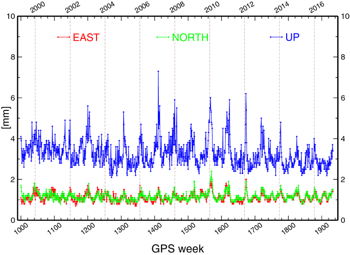
Weighted weekly RMS series of the combined solution showing separately the East, North, and Up components. No relative biases are seen between the East and North components and no increase with time as more new stations are involved in the cumulative solution
-
(2)
Comparison of the latest ITRF2014 solution and this densification solution in terms of positions and velocities in the common stations shown in Figs. 7 and 8,
Fig. 7 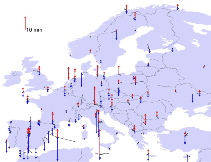
Position differences at epoch 2010 between ITRF2014 and D1933 in the common points. Blue and red arrows correspond to UP, while black arrows for 2D differences
Fig. 8 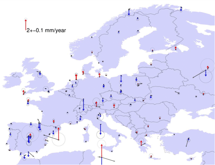
Velocity differences between ITRF2014 and D1933 solutions in the common points. Blue and red arrows correspond to UP, while black arrows for 2D differences
-
(3)
Browsing the individual residual times series of the stations.


Items 1–2 are useful to check and detect any biases in the solution in general, and item 3 is necessary to check each station for remaining outliers, offsets or any conflicts in overlapping cases.
The weighted RMS series shown in Fig. 6 clearly demonstrates the high quality and stability of the solution. The average WRMS for the East and North components are 1.1 mm, while 3.5 mm for the UP component. No increase in the WRMS can be observed around GPS week 1400 when the inclusion of the densification networks gradually starts. Some seasonality is still present in the series mainly due to the Nordic stations, where the snow accumulation on the antennae causes apparent temporary position biases during wintertime, although at several extreme cases, such as KIRU, KIR0, KUUS, SODA, VAAS, those data periods were removed before the final combination.
Figures 7 and 8 illustrate the position and the corresponding velocity differences, between the ITRF2014 reference frame solution and the D1933 densification solution. The plots demonstrate the successful alignment of the multi-year solution to the ITRF2014; no systematic biases are observed in the position or in the velocity estimates.
The standard deviations of the 14 transformation parameters between ITRF2014 and D1933, i.e., translation (tr), rotation (rot), scale (sc), for the positions and velocities are as follows: trX = 0.04 mm, trY = 0.04 mm, trZ = 0.04 mm, SC = 0.005 ppb, rotX = 0.012 mas, rotY = 0.016 mas, and rotZ = 0.011 mas.
D1933 is considered to be a high-quality, homogeneous, dense position and velocity data set aligned to ITRF2014 and created under full compliance with EUREF standards. The position estimates of the D1933 solution can be used for the validation and inter-comparison of official national ETRS89 positions used for the practical geodetic applications of the CORS networks.
Velocity field
An important product of the EPN Densification is the estimated velocity field, which has multiple scientific applications. At the European level, within the EUREF community the discussion has just started about the future introduction of semi-kinematic or kinematic reference frame realization, where the dense velocity field may effectively support the kinematic modeling. On the other hand, the homogeneous, dense velocity field from Svalbard to Crete shall be used as a reference from large to local scale or inter-regional interpretations and strain modeling.
The estimated 2D and UP velocity fields of the D1933 solution are shown in Figs. 9 and 10, respectively. In both cases, only the velocities of stations with more than 3 years of time series are plotted. As it is widely known that for achieving reliable velocity estimate in ideal cases observation series of at least 2.5 years are needed to reduce the bias that may be caused by apparent seasonal cycles (Blewitt and Lavallée 2002). Velocity estimate based on shorter series are most likely biased and in the presence of heightened noise level, the required time span should be considerably longer. This is especially valid for the UP component. Considering all arguments, we exclusively publish station positions and velocities based on longer than 3 years of observations.

Estimated horizontal velocities of the D1933 densification solution, expressed in the ETRF2000 reference frame. Velocities for stations with less than 3 years of observation history are not displayed but indicated with green dots to show the potential in the later updates
The 2D velocities in Fig. 9 are expressed in the ETRF2000 reference frame. We do easily distinguish the stable part of the continent and the active regions in the Mediterranean and Fennoscandia. The height variations are shown in Fig. 10, where we can also easily identify the main patterns: (1) large regions, where the general subsidence is primarily due to the sediment compaction, (2) Fennoscandian and Scottish post-glacial uplift, and (3) the moderate rise of the Alps and the Southern Apennines. The detailed interpretation of the tectonic patterns that may be observable in the data set is out of the scope of this paper. The delivered high-quality and fully homogeneous position and velocity solution, however, is offered to be used as reference for such geophysical studies.

Estimated UP velocities of the D1933 densification solution. Velocities for stations with less than 3 years of observation history are not displayed but indicated with green dots to show the potential in the later updates. Error ellipses are not shown here for the clarity of the figure
Despite the elimination of the velocities based on less than 3 years of data, both maps show some stations with velocities affected by local conditions, which are not well representing their tectonic environment. Assuming that the data analysis had been done correctly, corresponding to station time series without noisy sections and all offsets had been identified, the station specific biases may group as small- to medium-scale anthropogenic effects and monumentation issues. Water extraction and mining mostly cause locally significant, easily identifiable biases; stations such as Lorca in Spain, Katowice in Poland, Cluj in Romania, and Karaman in Turkey are removed from Figs. 9 and 10. As a lot of permanent GNSS stations are installed on buildings, the occasional instability of the building or the monument itself may distort the velocity estimation at a level of 1 mm/year or less. Such biases can be identified and marked using careful mathematical testing including geophysical information in the background. Assuming that on a given tectonic unit the 2D velocity pattern can be described as a spherical rotation and the residual velocities within a threshold should be considered as zero, then efficient and reliable filtering can be designed. Such filtering could be critically important in regions with lower tectonic activity, where the separation of the real signal and the (sub-)millimeter-level biases is essential to suppress velocities which are apparently do not represent the displacement field of the actual tectonic unit. Such velocity separation approach and its results will be treated in later.
Summary and outlook
We presented the integration of dense, national permanent GNSS network position solutions based on the long-term, homogeneous processing results, provided by agencies all over Europe. Daily and weekly position SINEX solutions were used as input, and through a multi-level testing and homogenization process a multi-year position and velocity solution, called D1933, has been created. This solution integrates 31 network solutions on the weekly position SINEX level including 3192 stations with observation length of 0.5–16 years.
D1933 is expressed in ITRF2014, ETRF2000, and ETRF2014 reference frames. The preparatory steps and final combinations were done with the CATREF software applying the Minimum Constraint approach using the ITRF2014 as reference frame solution. The comparison of ITRF2014 and D1933 shows an RMS agreement better than 1.5 mm 2D position and 0.2 mm/year 2D velocity. The position and velocity RMS agreement for the UP component are 3.2 mm and 0.4 mm/year, respectively. The EPN Densification results are published on the EPN Central Bureau website (http://www.epncb.oma.be/_densification/). It includes the lists and descriptions of the stations (log files, meta-data, station equipment) and the results in graphical and numeric form.
EPN Densification will play a significant role in the future. Two main European-scale initiatives should be mentioned: (1) EPOS ERIC, starting its operational work in 2019, (2) European Ground Motion Service (EU-GMS), starts action in 2020.
EPOS ERIC is a pan-European research infrastructure serving Solid Earth Science with contributions from observation networks covering several disciplines: seismology, volcanology, Near-Fault Observatories, and GNSS networks will be distributed in the frame of EPOS Thematic and Integrated Core Services. The presented European-scale combination will be part of the GNSS services and deliver times series and station velocities to EPOS.
EU-GMS targets the realization and maintenance of the European level map of surface motions derived from long-term satellite radar interferometric (PS-InSAR) data analysis. As PS-InSAR is a relative technique, a homogeneous continental-scale height velocity database is needed as a reference and to serve as ground truth to connect the independently obtained patches of relative motions derived from series of satellite radar images. The EPN Densification, with homogeneous coverage and realization, should be the ideal tool for this purpose.
These two initiatives warrant the continuity of EPN Densification, the continuation of the position SINEX collection and extension of the network. Since presently about 20% of the stations have less than 3 years of observations, the continuation will certainly improve and extend the velocity field. The next update of the EPN Densification results is expected in 2019 and regular updates are planned after that.
References
Altamimi Z, Collilieux X (2009) IGS contribution to the ITRF. J Geod 83(3–4):375–383. https://doi.org/10.1007/s00190-008-0294-1
Altamimi Z, Sillard P, Boucher C (2002) ITRF2000: a new release of the International Terrestrial Reference Frame for earth science applications. J Geophys Res 107(B10):2214. https://doi.org/10.1029/2001JB000561
Altamimi Z, Sillard P, Boucher C (2007) CATREF software: combination and analysis of terrestrial reference frames. LAREG Technical, Institut Géographique National, Paris
Altamimi Z, Rebischung P, Métivier L, Collilieux X (2016) ITRF2014: a new release of the International Terrestrial Reference Frame modeling nonlinear station motions. J Geophys Res 121(8):6019–6131. https://doi.org/10.1002/2016JB013098
Blewitt G, Lavallée D (2002) Effect of annual signals on geodetic velocity. J Geophys Res 107(B7):ETG9-1–ETG9-11. https://doi.org/10.1029/2001jb000570
Bruyninx C, Habrich H, Söhne W, Kenyeres A, Stangl G, Völksen C (2012) Enhancement of the EUREF permanent network services and products. In: Kenyon S, Pacino M, Marti U (eds) Geodesy for planet earth, international association of geodesy symposia, vol 136. Springer, Berlin, pp 27–35. https://doi.org/10.1007/978-3-642-20338-1_4
Bruyninx C et al (2013) IAG WG SC1.3 on regional dense velocity fields: first results and steps ahead. In: Altamimi Z, Collilieux X (eds) Reference frames for applications in geosciences, international association of geodesy symposia, vol 138. Springer, Berlin, pp 137–145. https://doi.org/10.1007/978-3-642-32998-2_22
Dach R, Lutz S, Walser P, Fridez P (eds) (2015) Bernese GNSS software version 5.2. User manual. Astronomical Institute, University of Bern, Bern Open Publishing, Bern. https://doi.org/10.7892/boris.72297. ISBN 978-3-906813-05-9
Davies P, Blewitt G (2000) Methodology for global geodetic time series estimation: a new tool for geodynamics. J Geophys Res 105(B5):11083–11100. https://doi.org/10.1029/2000JB900004
Devoti R et al (2017) A combined velocity field of the mediterranean region. Ann Geophys 60(2):S0215. https://doi.org/10.4401/ag-7059
Hefty J (2007) Geo-kinematics of central and southern-East Europe resulting from combination of various regional GPS velocity fields. Acta Geodyn Geomater 4(4):173–189
IERS Message 103 (2006) http://www.iers.org/documents/ac/sinex/sinex_v202.pdf. Accessed 4 Dec 2006
Jeffery KG, Bailo D (2014) EPOS: using metadata in geoscience. In: Closs S, Studer R, Garoufallou E, Sicilia MA (eds) Metadata and semantics research. MTSR 2014. Communications in computer and information science, vol 478. Springer, Cham, pp 170–184. https://doi.org/10.1007/978-3-319-13674-5_17
King RW, Bock Y (1996) Documentation of the GAMIT GPS analysis software version 9.3. Massachusetts Institute of Technology, Cambridge
Kreemer C, Blewitt G, Klein EC (2014) A geodetic plate motion and global strain rate model. Geochem Geophys Geosyst 15(10):3849–3889
Legrand J, Bruyninx C, Craymer M, Dawson J, Griffiths J, Kenyeres A, Rebischung P, Sanchez L, Santamaría-Gómez A, Saria E, Altamimi Z (2014) IAG WG “integration of dense velocity fields in the ITRF” combination of regional solutions toward a global velocity field. In: van Dam T (ed) Reference frames for applications in geosciences (REFAG2014), international association of geodesy symposia, vol 146. Springer, Berlin
Nocquet JM, Calais E (2003) Crustal velocity field of western Europe from permanent GPS array solutions, 1996–2001. Geophys J Int 154(1):72–88. https://doi.org/10.1046/j.1365-246X.2003.01935.x
Rebischung P (2011) Upcoming switch to IGS08/igs08.atx, IGSMAIL no. 6354, 7th March
Sánchez L, Drewes H, Brunini C, Mackern MV, Martínez-Díaz W (2015) SIRGAS core network stability. In: Rizos C, Willis P (eds) IAG 150 years. International association of geodesy symposia, vol 143. Springer, Cham. https://doi.org/10.1007/1345_2015_143
Savage JC (2018) Euler-vector clustering of GPS velocities defines microplate geometry in southwest Japan. J Geophys Res 123(2):1954–1968. https://doi.org/10.1002/2017JB014874
Sillard P, Boucher C (2001) A review of algebraic constraints in terrestrial reference frame datum definition. J Geod 75(2–3):63–73. https://doi.org/10.1007/s001900100166
Zumberge JF, Heflin MB, Jefferson DC, Watkins MM, Webb FH (1997) Precise point positioning for the efficient and robust analysis of GPS data from large networks. J Geophys Res 102(B3):5005–5017. https://doi.org/10.1029/96JB03860
Acknowledgements
Open access funding provided by Lechner Non-profit Ltd. The related research work was supported by the Hungarian Research Fund (OTKA) under contract # K109464. The work done at the EPNCB to implement and maintain the EPN Densification web pages is highly appreciated and acknowledged. Institutions supporting the related work of EPN Densification are listed in affiliation section.
Author information
Authors and Affiliations
Corresponding author
Additional information
Publisher's Note
Springer Nature remains neutral with regard to jurisdictional claims in published maps and institutional affiliations.
Rights and permissions
Open Access This article is distributed under the terms of the Creative Commons Attribution 4.0 International License (http://creativecommons.org/licenses/by/4.0/), which permits unrestricted use, distribution, and reproduction in any medium, provided you give appropriate credit to the original author(s) and the source, provide a link to the Creative Commons license, and indicate if changes were made.
About this article

Cite this article
Kenyeres, A., Bellet, J.G., Bruyninx, C. et al. Regional integration of long-term national dense GNSS network solutions. GPS Solut 23, 122 (2019). https://doi.org/10.1007/s10291-019-0902-7
Received:
Accepted:
Published:
DOI: https://doi.org/10.1007/s10291-019-0902-7