Towards Massively Parallel Computations in Algebraic Geometry

Abstract

Introducing parallelism and exploring its use is still a fundamental challenge for the computer algebra community. In high-performance numerical simulation, on the other hand, transparent environments for distributed computing which follow the principle of separating coordination and computation have been a success story for many years. In this paper, we explore the potential of using this principle in the context of computer algebra. More precisely, we combine two well-established systems: The mathematics we are interested in is implemented in the computer algebra system Singular, whose focus is on polynomial computations, while the coordination is left to the workflow management system GPI-Space, which relies on Petri nets as its mathematical modeling language and has been successfully used for coordinating the parallel execution (autoparallelization) of academic codes as well as for commercial software in application areas such as seismic data processing. The result of our efforts is a major step towards a framework for massively parallel computations in the application areas of Singular, specifically in commutative algebra and algebraic geometry. As a first test case for this framework, we have modeled and implemented a hybrid smoothness test for algebraic varieties which combines ideas from Hironaka’s celebrated desingularization proof with the classical Jacobian criterion. Applying our implementation to two examples originating from current research in algebraic geometry, one of which cannot be handled by other means, we illustrate the behavior of the smoothness test within our framework and investigate how the computations scale up to 256 cores.

1 Introduction

Experiments based on calculating examples have always played a key role in mathematical research. Advanced hardware structures paired with sophisticated mathematical software tools allow for far reaching experiments which were previously unimaginable. In the realm of algebra and its applications, where exact calculations are inevitable, the desired software tools are provided by computer algebra systems. In order to take full advantage of modern multicore computers and high-performance clusters, the computer algebra community must provide parallelism in their systems. This will boost the performance of the systems to a new level, thus extending the scope of applications significantly. However, while there has been a lot of progress in this direction in numerical computing, achieving parallelization in symbolic computing is still a tremendous challenge both from a mathematical and technical point of view.

On the mathematical side, there are some algorithms whose basic strategy is inherently parallel, whereas many others are sequential in nature. The systematic design and implementation of parallel algorithms (see, e.g., [5,6,7]) is a major task for the years to come. On the technical side, models for parallel computing have long been studied in computer science. These differ in several fundamental aspects. Roughly, two basic paradigms can be distinguished according to assumptions on the underlying hardware. The shared memory-based models allow several different computational processes (called threads) to access the same data in memory, while the distributed models run many independent processes which need to communicate their progress to one or several of the other processes. Creating the prerequisites for writing parallel code in a computer algebra system originally designed for sequential processes requires considerable efforts which affect all levels of the system.

In this paper, we explore an alternative way of introducing parallelism into computer algebra computations. This approach is non-intrusive and allows for distributed computing. It is based on the principle of separating coordination and computation, a principle which has already been pursued with great success in high-performance numerical simulation. Specifically, we rely on the workflow management system GPI-Space [43] for coordination, while the mathematics we are interested in is implemented in the computer algebra system Singular [15].

Singular is under development at TU Kaiserslautern, focuses on polynomial computations, and has been successfully used in application areas such as algebraic geometry and singularity theory. GPI-Space, on the other hand, is under development at Fraunhofer ITWM Kaiserslautern and has been successfully used for coordinating the parallel execution (autoparallelization) of academic codes as well as for commercial software in application areas such as seismic data processing. As its mathematical modeling language, GPI-Space relies on Petri nets, which are specifically designed to model concurrent systems and yield both data parallelism and task parallelism. In fact, GPI-Space is not only able to automatically balance, to automatically scale up to huge machines, or to tolerate machine failures, but can also use existing legacy applications and integrate them, without requiring any change to them. In our case, Singular calls GPI-Space, which, in turn, manages several (many) instances of Singular in its existing binary form (without any need for changes). The experiments carried through so far are promising and indicate that we are on our way towards a convenient framework for massively parallel computations in Singular.

One of the central tasks of computational algebraic geometry is the explicit construction of objects with prescribed properties, for instance, to find counterexamples to conjectures or to construct general members of moduli spaces. Arguably, the most important property to be checked here is smoothness. Classically, this means to apply the Jacobian criterion: If $X\subset {\mathbb {A}}^n_{{\mathbb {K}}}$ (respectively, $X\subset {\mathbb {P}}^n_{{\mathbb {K}}}$) is an equidimensional affine (respectively, projective) algebraic variety of dimension d with defining equations $f_1=\cdots =f_s=0$, compute a Gröbner basis of the ideal generated by the $f_i$ together with the $(n-d)\times (n-d)$ minors of the Jacobian matrix of the $f_i$ in order to check whether this ideal defines the empty set. The resulting process is predominantly sequential. It is typically expensive (if not unfeasible), especially in cases where the codimension $n-d$ is large.

In [8], an alternative smoothness test has been suggested by the first and third author (see [9] for the implementation in Singular). This test builds on ideas from Hironaka’s celebrated desingularization proof [26] and is intrinsically parallel. To explore the potential of our framework, we have modeled and implemented an enhanced version of the test (see Remark 28 for a description of the most significant improvements). Following [8], we take our cue from the fact that each smooth variety is locally a complete intersection. Roughly, to check the smoothness of a given affine variety $X\subset {\mathbb {A}}^n_{{\mathbb {K}}}$, the idea is then to apply Hironaka’s method of descending induction by hypersurfaces of maximal contact (in its constructive version by Bravo, Encinas, and Villamayor [13]). This allows us either to detect non-smoothness during the process, or to finally realize a finite covering of X by affine charts such that in each chart, X is given as a smooth complete intersection. More precisely, at each iteration step, our algorithm starts from finitely many affine charts $U_i\subset {\mathbb {A}}^n_{{\mathbb {K}}}$ whose union contains X, together with varieties $W_i\subset {\mathbb {A}}^n_{{\mathbb {K}}}$ and embeddings $X\cap U_i\subset W_i\cap U_i$ such that each $W_i\cap U_i$ is a smooth complete intersection in $U_i$. Providing a constructive version of Hironaka’s termination criterion, the algorithm then either detects that X is singular in one $U_i$, and terminates, or constructs for each i finitely many affine charts $U'_{ij}\subset {\mathbb {A}}^n_{{\mathbb {K}}}$ whose union contains $X\cap U_i$, together with varieties $W'_{ij}\subset W_i$ and embeddings $X\cap U'_{ij}\subset W'_{ij}\cap U'_{ij}$ such that each $W'_{ij}\cap U'_{ij}$ is a smooth complete intersection in $U'_{ij}$ whose codimension is one less than that of $X\cap U_i$ in $W_i\cap U_i$. Since at each step, the computations in one chart do not depend on results from the other charts, the algorithm is indeed parallel in nature. Moreover, since our implementation branches into all available choices of charts in a massively parallel way and terminates once X is completely covered by charts, it will automatically determine a choice of charts which leads to the smoothness certificate in the fastest possible way.

In fact, there is one more twist: As experiments show, see [8], the smoothness test is most effective in a hybrid version which makes use of the above ideas to reduce the general problem to checking smoothness in finitely many embedded situations $X\cap U\subset W\cap U$ of low codimension, and applies (a relative version of) the Jacobian criterion there.

Our paper is organized as follows. In Sect. 2, we briefly review smoothness and recall the Jacobian criterion. In Sect. 3, we summarize what we need from Hironaka-style desingularization and develop our smoothness test. Section 4 contains a discussion of GPI-Space and Petri nets which prepares for Sect. 5, where we show how to model our test in terms of Petri nets. This forms the basis for the implementation of the test using Singular within GPI-space. Finally, in Sect. 6, we illustrate the behavior of the smoothness test and its implementation by checking two examples from current research in algebraic geometry. These examples are surfaces of general type, one of which cannot be handled by other means.

We would like to thank the anonymous referees for their valuable remarks.

2 Smoothness and the Jacobian Criterion

We describe the geometry behind our algorithm in the classical language of algebraic varieties over an algebraically closed field. Because smoothness is a local property, and each quasiprojective (algebraic) variety admits an open affine covering, we restrict our attention to affine (algebraic) varieties.

Let ${{\mathbb {K}}}$ be an algebraically closed field. Write ${\mathbb {A}}^n_{{{\mathbb {K}}}}$ for the affine n-space over ${{\mathbb {K}}}$. An affine variety (over ${{\mathbb {K}}}$) is the common vanishing locus $V(f_1, \dots , f_r)\subset {\mathbb {A}}^n_{{{\mathbb {K}}}}$ of finitely many polynomials $f_i\in {{\mathbb {K}}}[x_1,\dots , x_n]$. If Z is such a variety, let

$$\begin{aligned} I_Z=\{f\in {{\mathbb {K}}}[x_1,\ldots ,x_n] \mid f(p)=0 \text { for all } p\in Z\}\subset {{\mathbb {K}}}[x_1,\ldots ,x_n] \end{aligned}$$

be its vanishing ideal, let ${{\mathbb {K}}}[Z]={{\mathbb {K}}}[x_1,\ldots ,x_n]/I_Z$ be its ring of polynomial functions, and let $\dim Z = \dim {{\mathbb {K}}}[Z]$ be its dimension.

Given a polynomial $h\in {{\mathbb {K}}}[x_1,\ldots ,x_n]$, we write

$$\begin{aligned} D(h) = \mathbb A^n_{{{\mathbb {K}}}}{\setminus } V(h)=\{p\in {\mathbb {A}}^n_{{{\mathbb {K}}}} \mid h(p) \ne 0\} \end{aligned}$$

for the principal open subset of ${\mathbb {A}}^n_{{{\mathbb {K}}}}$ defined by h, and ${\mathcal {O}}_{Z}(Z\cap D(h))$ for the ring of regular functions on $Z\cap D(h)$. If $p\in Z$ is a point, we write $\mathcal {O}_{Z,p}$ for the local ring of Z at p, and ${\mathfrak {m}}_{Z,p}$ for the maximal ideal of $\mathcal {O}_{Z,p}$. Recall that both rings ${\mathcal {O}}_{Z}(Z\cap D(h))$ and $\mathcal {O}_{Z,p}$ are localizations of ${{\mathbb {K}}}[Z]$: Allow powers of the polynomial function defined by h on Z and polynomial functions on Z not vanishing at p as denominators, respectively.

Relying on the trick of Rabinowitch, we regard $Z\cap D(h)$ as an affine variety: If $I_Z=\langle f_1,\dots , f_s\rangle$, identify $Z\cap D(h)$ with the vanishing locus

$$\begin{aligned} V(f_1,\dots , f_s, ht-1)\subset {\mathbb {A}}^{n+1}_{{{\mathbb {K}}}}, \end{aligned}$$

where t is an extra variable.

The tangent space at a point $p=(a_1,\dots , a_n)\in Z$ is the linear variety

$$\begin{aligned} T_p Z = V(d_p(f) \mid f\in I_Z)\subset {\mathbb {A}}^n_{{{\mathbb {K}}}}, \end{aligned}$$

where $d_pf$ is the differential of f at p:

$$\begin{aligned} d_p f=\sum _{i=1}^n \frac{\partial f}{\partial x_i}(p)(x_i-a_i) \in {{\mathbb {K}}}[x_1,\dots , x_n]. \end{aligned}$$

We have

$$\begin{aligned} \dim T_p Z \ge \max \{\dim V \mid V \text { is an irreducible component of } Z \text { through } p\}, \end{aligned}$$

and say that Z is smooth at p if these numbers are equal. Equivalently, $\mathcal {O}_{Z,p}$ is a regular local ring. Otherwise, Z is singular at p. The variety Z is smooth if it is smooth at each of its points.

Recall that a variety Z is equidimensional if all its irreducible components have the same dimension. Algebraically, this means that the ideal $I_Z$ is equidimensional; that is, all associated primes of $I_Z$ have the same dimension.

Theorem 1

(Jacobian Criterion) Let ${{\mathbb {K}}}$ be an algebraically closed field, and let $Z = V(f_1, \dots , f_s)\subset {\mathbb {A}}^n_{{{\mathbb {K}}}}$ be an affine variety which is equidimensional of dimension d. Write $I_{n-d}\left( {{\mathcal {J}}}\right)$ for the ideal generated by the $(n-d) \times (n-d)$ minors of the Jacobian matrix ${{\mathcal {J}}} = \left( {\partial f_i \over \partial x_j}\right)$. If $I_{n-d}\left( {{\mathcal {J}}}\right) +I_Z = \langle 1\rangle$, then Z is smooth, and the ideal $\langle f_1, \dots , f_s\rangle \subset {{\mathbb {K}}}[x_1,\ldots ,x_n]$ is equal to the vanishing ideal $I_Z$ of Z. In particular, $\langle f_1, \dots , f_s\rangle$ is a radical ideal.

If $Y\subset Z\subset {\mathbb {A}}^n_{{{\mathbb {K}}}}$ are two affine varieties, the vanishing ideal $I_{Y,Z}$ of Y in Z is the ideal generated by $I_Y$ in ${{\mathbb {K}}}[Z]$. If Z is equidimensional, we write ${\text {codim}}_Z Y=\dim Z - \dim Y$ for the codimension of Y in Z, and say that Y is a complete intersection in Z if $I_{Y,Z}$ can be generated by ${\text {codim}}_Z Y={\text {codim}}\, I_{Y,Z}$ elements (then Y and $I_{Y,Z}$ are equidimensional as well).

3 A Hybrid Smoothness Test

In this section, we present the details of our hybrid smoothness test which, as already outlined in Introduction, combines the Jacobian criterion with ideas from Hironaka’s landmark paper on the resolution of singularities [26] in which Hironaka proved that such resolutions exist, provided we work in characteristic zero.

For detecting non-smoothness and controlling the resolution process, Hironaka developed a theory of standard bases for local rings and their completions (see [23, Chapter 1] for the algorithmic aspects of standard bases). Based on this, he defined several invariants controlling the desingularization process. The so-called $\nu ^{*}$-invariant generalizes the order of a power series. As some sort of motivation, we recall its definition in the analytic setting: Let $(X,0) \subset ({{\mathbb {A}}}_{{{\mathbb {K}}}}^{n},0)$ be an analytic space germ over an algebraically closed field ${{\mathbb {K}}}$ of characteristic zero, let ${{\mathbb {K}}}\{x_{1},\ldots ,x_{n}\}$ be the ring of convergent power series with coefficients in ${{\mathbb {K}}}$, and let $I_{X,0} \subset {{\mathbb {K}}}\{x_{1},\ldots ,x_{n}\}$ be the defining ideal of (X, 0). If $f_{1},\dots ,f_{s}$ form a minimal standard basis of $I_{X,0}$, and the $f_i$ are sorted by increasing order ${\text {ord}}(f_i)$, then set

$$\begin{aligned} \nu ^{*}(X,0) = ({\text {ord}}(f_1), \dots , {\text {ord}}(f_s)). \end{aligned}$$

This invariant is the key to Hironaka’s termination criterion: The germ (X, 0) is singular iff at least one of the entries of $\nu ^{*}(X,0)$ is $>1$.

In the algebraic setting of this paper, let $X\subset {{\mathbb {A}}}_{{{\mathbb {K}}}}^{n}$ be an equidimensional affine variety, with vanishing ideal $I_X\subset {{\mathbb {K}}}[x_1,\ldots ,x_n]$, where ${{\mathbb {K}}}$ is an algebraically closed field of arbitrary characteristic. Working in arbitrary characteristic allows for a broader range of potential applications and is not a problem since we will only rely on results from Hironaka’s papers which also hold in positive characteristic.

To formulate Hironaka’s criterion in the algebraic setting, we first recall how to extend the notion of order:

Definition 2

If $(R, {\mathfrak {m}})$ is any local Noetherian ring, and $0\ne f\in R$ is any element, then the order of f is defined by setting

$$\begin{aligned} {\text {ord}}(f)=\max \{k\in {\mathbb {N}}\mid f\in {\mathfrak {m}}^k\}. \end{aligned}$$

Definition 3

([26, 27]) With notation as above, let $p\in X$. If $f_{1},\dots ,f_{s}$ form a minimal standard basis of the extended ideal $I_X {{\mathcal {O}}}_{{{\mathbb {A}}}^n_{{{\mathbb {K}}}},p}$ with respect to a local degree ordering, and the $f_i$ are sorted by increasing order, set

$$\begin{aligned} \nu ^{*}(X,p) = ({\text {ord}}(f_1), \dots , {\text {ord}}(f_s)). \end{aligned}$$

Lemma 4

([26, 27]) The sequence $\nu ^{*}(X,p)$ depends only on X and p.

Remark 5

Note that $\nu ^{*}(X,p)$ can be determined algorithmically: A minimal standard basis as required is obtained by translating p to the origin and applying Mora’s tangent cone algorithm (see [23, 36, 39, 40]).

Hironaka’s criterion can now be stated as follows:

Lemma 6

([26], Chapter III) The variety X is singular at $p\in X$ iff

$$\begin{aligned} \nu ^{*}(X,p) >_{{\text {lex}}} (1,\dots ,1)\in {\mathbb {N}}^{{\text {codim}} X}, \end{aligned}$$

(1)

where $>_{{\text {lex}}}$ denotes the lexicographical ordering.

Note that if X is singular at p, then the length of $\nu ^{*}(X,p)$ may be larger than ${\text {codim}}(X)$, but at least one of the first ${{\text {codim}}(X)}$ entries will be $>1$.

Hironaka’s criterion is not of immediate practical use for us: We cannot examine each single point $p\in X$. Fortunately, solutions to this problem have been suggested by various authors while establishing constructive versions of Hironaka’s resolution process (see, for example, [4, 13, 18, 50]). Here, we follow the approach of Bravo, Encinas, and Villamayor [13] which is best-suited for our purposes. Their simplified proof of desingularization replaces local standard bases at individual points by the use of loci of maximal order. These loci are obtained by polynomial computations in finitely many charts (see [19, Section 4.2]). Loci of maximal order can be used to find so-called hypersurfaces of maximal contact, which again only exist locally in charts. In a Hironaka style resolution process, hypersurfaces of maximal contact allow for a descending induction on the dimension of the respective ambient space. That such hypersurfaces generally do not exist in positive characteristic is a key obstacle for extending Hironaka’s ideas to positive characteristic [24].

In our context, we encounter a particularly simple special case:

Notation 7

From now on, we suppose that we are given an embedding $X\subset W$, where W is a smooth complete intersection in ${{\mathbb {A}}}_{{{\mathbb {K}}}}^{n}$, say of codimension r. In particular, W is equidimensional of dimension

$$\begin{aligned} d=n-r. \end{aligned}$$

The idea is then to first check whether the locus of order at least two is non-empty. In this case, X is singular. Otherwise, we can find a finite covering of X by affine charts and in each chart a hypersurface of maximal contact whose construction relies only on the suitable choice of one of the generators of $I_X$ together with one first-order partial derivative of this generator.¹ In each chart, we then consider the hypersurface of maximal contact as the new ambient space of X and proceed by iteration.

The resulting process allows us to decide at each step of the iteration whether there is a point $p\in X$ such that the next entry of $\nu ^{*}(X,p)$ is $\ge 2$. To give a more precise statement, we suppose that X has positive codimension in W (otherwise, X is necessarily smooth). Crucial for obtaining information on an individual entry of $\nu ^{*}$ is the order of ideals:

Definition 8

If $(R, {\mathfrak {m}})$ is any local Noetherian ring, and $\langle 0 \rangle \ne J=\langle h_1,\dots ,h_t\rangle \subset R$ is any ideal, then the order of J is defined by setting

$$\begin{aligned} {\text {ord}}(J)=\max \{k\in {\mathbb {N}}\mid J\subset {\mathfrak {m}}^k\} ={\text {min}}\left\{ {\text {ord}}(h_i) \mid i=1,\dots , t\right\} . \end{aligned}$$

In our geometric setup, we apply this as follows: Given an ideal $\langle 0 \rangle \ne I\subset {{\mathbb {K}}}[W]$ and a point $p\in W$, the order ${\text {ord}}_p(I)$ of I at p is defined to be the order of the extended ideal $I {\mathcal {O}}_{W,p}$. For $0\ne f\in {{\mathbb {K}}}[W]$ we similarly define ${\text {ord}}_p(f)$ as the order of the image of f in ${\mathcal {O}}_{W,p}$.

Definition 9

With notation as above, for any integer $b \in {{\mathbb {N}}}$, the locus of order at least b of the vanishing ideal $I_{X,W}$ is

$$\begin{aligned} {\text {Sing}}(I_{X,W},b)=\left\{ p\in X\mid {\text {ord}}_{p}(I_{X,W})\ge b\right\} . \end{aligned}$$

Remark 10

([26], Chapter III) Note that the loci ${\text {Sing}}(I_{X,W},b)$ are Zariski closed since the function

$$\begin{aligned} X\rightarrow {\mathbb {N}}, \ p \mapsto {\text {ord}}_{p}(I_{X,W}), \end{aligned}$$

is Zariski upper semi-continuous.

Remark 11

With notation as above, let a point $p\in X$ be given. Then, the first r elements of a minimal standard basis of $I_X {{\mathcal {O}}}_{{{\mathbb {A}}}^n_{{\mathbb {K}}},p}$ as in Definition 3 must have order 1 by our assumptions on W, that is, the first r entries of $\nu ^*(X,p)$ are equal to 1. On the other hand, if ${\text {ord}}_{p}(I_{X,W})\ge 2$, then the $(r+1)$-st entry of $\nu ^*(X,p)$ is $\ge 2$. Hence, in this case, X is singular at p since the codimension of X in ${\mathbb {A}}_{{{\mathbb {K}}}}^{n}$ is at least $r+1$ by our assumptions.

In terms of loci of order at least two, this amounts to:

Lemma 12

With notation as above, X is singular if

$$\begin{aligned} {\text {Sing}}(I_{X,W},2)\not =\emptyset . \end{aligned}$$

Proof

Clear from Remark 11. $\square$

To determine the loci ${\text {Sing}}(I_{X,W},b)$ in a Zariski neighborhood of a point $p\in X$ explicitly, derivatives with respect to a regular system of parameters of W at p are the method of choice: See [13, p. 404] for characteristic zero, and [22, Sections 2.5 and 2.6] for positive characteristic using Hasse derivatives. For a more detailed description, fix a point $p\in W$. According to our assumptions, the local ring $\mathcal {O}_{W,p}$ is regular of dimension d. So we can find a regular system of parameters $X_{1,p},\dots , X_{d,p}$ for $\mathcal {O}_{W,p}$. That is, $X_{1,p},\dots , X_{d,p}$ form a minimal set of generators for ${\mathfrak {m}}_{W,p}$. By the Cohen structure theorem, we may, thus, think of the completion $\widehat{{\mathcal {O}}_{W,p}}$ as a formal power series ring in d variables (see [17, Proposition 10.16]): The map

$$\begin{aligned} \varPhi :{{\mathbb {K}}}[[y_1, \dots , y_d]] \rightarrow \widehat{{\mathcal {O}}_{W,p}}, \ y_i\mapsto X_{i,p}, \end{aligned}$$

is an isomorphism of local rings. In particular, the order of an element $f\in {{\mathbb {K}}}[W]$ at p coincides with the order of the formal power series $\varPhi ^{-1}(f)\in {{\mathbb {K}}}[[y_1, \dots , y_d]]$. The latter, in turn, can be computed as follows:

Lemma 13

([13, 22]) Let $R={{\mathbb {K}}}[[y_1,\dots ,y_d]]$, let ${{\mathfrak {m}}}=\langle y_1,\dots ,y_d \rangle$ be the maximal ideal of R, and let $F\in R {\setminus } \{0\}$. Then,

$$\begin{aligned} {\text {ord}}(F)= {\text {min}}\left\{ m \in {{\mathbb {N}}} \bigm | \frac{\partial ^{a} F}{\partial y^{a}}\not \in {{\mathfrak {m}}} \text { for some } a \in {{\mathbb {N}}}^n \text { with } |a|=m \right\} , \end{aligned}$$

where the derivatives denote the usual formal derivatives in characteristic zero and Hasse derivatives in positive characteristic.

As we focus on the locus ${\text {Sing}}(I_{X,W},b)$ with $b=2$, only first-order formal derivatives play a role for us. Since these derivatives coincide with the first-order Hasse derivatives, we do not need to discuss Hasse derivatives here.

Definition 14

In the situation above, we use the isomorphism $\varPhi$ of the Cohen structure theorem to define first-order derivatives of elements $f\in \widehat{{\mathcal {O}}_{W,p}}$ with respect to the regular system of parameters $X_{1,p},\dots , X_{d,p}$: Set

$$\begin{aligned} \frac{\partial f}{\partial X_{j,p}}=\varPhi \quad \left( \frac{\partial \varPhi ^{-1}(f)}{\partial y_{j}}\right) \in \widehat{{\mathcal {O}}_{W,p}}, \text { for } j=1,\dots , d. \end{aligned}$$

We summarize our discussion so far. If $I_{X,W}$ is given by a set of generators $f_{r+1}, \dots , f_s\in {{\mathbb {K}}}[W]{\setminus } \{0\}$, and if $p\in X$, then $p\in {\text {Sing}}(I_{X,W},2)$ iff ${\text {ord}}_p(f_i)>1$ for all $i\in \{r+1,\dots ,s\}$. In this case, X is singular at p. Furthermore, if $0\ne f\in {{\mathbb {K}}}[W]$ is any element, $p\in W$ is any point, and $X_{1,p},\dots , X_{d,p}$ is a regular system of parameters for $\mathcal {O}_{W,p}$, then ${\text {ord}}_p(f)>1$ iff

$$\begin{aligned} 1 \not \in \varDelta _p(f) :=\left\langle f, \frac{\partial f}{\partial X_{1,p}},\dots , \frac{\partial f}{\partial X_{d,p}} \right\rangle _{\widehat{\mathcal {O}_{W,p}}}\subset \widehat{\mathcal {O}_{W,p}}. \end{aligned}$$

(2)

Now, as before, we cannot examine each point individually. The following arguments will allow us to remedy this situation in Lemma 20. We begin by showing that there is a locally consistent way of choosing regular systems of parameters:

Lemma 15

As before, let $I_W=\langle f_1,\dots ,f_r \rangle \subset {{\mathbb {K}}}[x_1,\dots ,x_n]$ be the ideal of the smooth complete intersection W. Let ${{\mathcal {J}}} = \left( {\partial f_i \over \partial x_j}\right)$ be the Jacobian matrix of $f_1,\dots ,f_r$. Then, there is a finite covering of W by principal open subsets D(h) of ${\mathbb {A}}_{{\mathbb {K}}}^n$ such that:

• 1. Each polynomial h is a maximal minor of ${{\mathcal {J}}}$.

• 2. For each h, the variables $x_j$ not used for differentiation in forming the minor h induce by translation a regular system of parameters for every local ring ${{\mathcal {O}}_{W,p}}$, $p\in W\cap D(h)$.

For each h, we refer to such a choice of a local system of parameters at all points of $W\cap D(h)$ as a consistent choice.

Proof

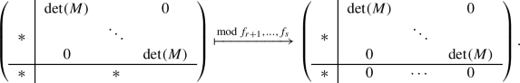
Consider a point $p_0\in W$. Then, by the Jacobian criterion, there is at least one minor $h=\det (M)$ of ${{\mathcal {J}}}$ of size r such that $h(p_0) \ne 0$ (recall that we assume that W is smooth). Suppose for simplicity that h involves the last r columns of ${{\mathcal {J}}}$, and let $p=(a_1,\dots ,a_n)$ be any point of $W\cap D(h)$. Then, the images of $x_{1}-a_{1}, \ldots ,x_d-a_d, f_1,\ldots ,f_r$ in ${{\mathcal {O}} _{{{\mathbb {A}}}^n_{{\mathbb {K}}},p}}$ are actually contained in ${{\mathfrak {m}}}_{{{\mathbb {A}}}^n_{{\mathbb {K}}},p}$ and represent a ${{\mathbb {K}}}$-basis of the Zariski tangent space ${{\mathfrak {m}}}_{{{\mathbb {A}}}^n_{{\mathbb {K}}},p}/{{\mathfrak {m}}}_{{{\mathbb {A}}}^n_{{\mathbb {K}}},p}^2$. Hence, by Nakayama’s lemma, they form a minimal set of generators for ${{\mathfrak {m}}}_{{{\mathbb {A}}}^n_{{\mathbb {K}}},p}$. Since $f_1,\dots ,f_r$ are mapped to zero when we pass to ${{\mathcal {O}}}_{W,p}$, the images of $x_{1}-a_{1}, \ldots ,x_d-a_d$ in ${{\mathcal {O}}}_{W,p}$ form a regular system of parameters for ${{\mathcal {O}}}_{W,p}$. The result follows because W is quasi-compact in the Zariski topology. $\square$

Notation 16

For further considerations, we retain the notation of the lemma and its proof. Fix one principal open subset $D(h) \subset {{\mathbb {A}}}^n_{{\mathbb {K}}}$ as in the lemma. Suppose that $h=\det (M)$ involves the last r columns of the Jacobian matrix ${{\mathcal {J}}}$. Furthermore, fix one element $0\ne f\in {{\mathbb {K}}}[W]$.

We now show how to find an ideal $\varDelta (f) \subset {{\mathcal {O}}}_{W}(W\cap D(h))$ such that

$$\begin{aligned} \varDelta (f)\;\! \widehat{\mathcal {O}_{W,p}}=\varDelta _p(f) \;\text { for each point }\; p\in W\cap D(h), \end{aligned}$$

where $\varDelta _p(f)$ is defined as in (2). Technically, we manipulate polynomials, starting from a polynomial in ${{\mathbb {K}}}[x_1,\dots ,x_n]$ representing f. By abuse of notation, we denote this polynomial again by f.

Construction 17

We construct a polynomial $\tilde{f}\in {{\mathbb {K}}}[x_1,\dots , x_n]$ whose image in ${{\mathcal {O}}}_{W}(W\cap D(h))$ coincides with that of f, and whose partial derivatives $\frac{\partial \tilde{f}}{\partial x_j}$, $j=d+1,\dots , n$, are mapped to zero in ${{\mathcal {O}}}_{W}(W\cap D(h))/\langle f \rangle$. For this, let A be the matrix of cofactors of M. Then,

$$\begin{aligned} A \cdot M = h \cdot E_{r}, \end{aligned}$$

where $E_r$ is the $r\times r$ identity matrix. Moreover, if $I\subset {{\mathbb {K}}}[x_1,\dots ,x_n]$ is the ideal generated by the entries of the vector $(\tilde{f_1},\dots ,\tilde{f}_{r})^T =A \cdot (f_1,\dots ,f_{r})^T$, then the extended ideals $I\mathcal {O}_{{{\mathbb {A}}}^n_{{\mathbb {K}}}}(D(h))$ and $I_W\mathcal {O}_{{{\mathbb {A}}}^n_{{\mathbb {K}}}}(D(h))$ coincide since h is a unit in $\mathcal {O}_{{{\mathbb {A}}}^n_{{\mathbb {K}}}}(D(h))$.

Let $\widetilde{{\mathcal {J}}}=\left( {\partial {\tilde{f_i}} \over \partial {x_j}}\right)$ be the Jacobian matrix of $\tilde{f_1},\dots ,\tilde{f}_{r}$. Then, the matrix obtained by restricting the entries of $\widetilde{{{\mathcal {J}}}}$ to $W\cap D(h)$ can be written as

$$\begin{aligned} \widetilde{{{\mathcal {J}}}}\vert _{W\cap D(h)} = \begin{pmatrix} \quad *&\mid&h \cdot E_{r}\end{pmatrix} \end{aligned}$$

(apply the product rule and reduce modulo $f_1,\dots , f_r$). In $\mathcal {O}_{{{\mathbb {A}}}^n_{{\mathbb {K}}}}(D(h))$, the polynomial ${\hat{f}}=h\cdot f$ represents the same class as f. Moreover, modulo f, each partial derivative of ${\hat{f}}$ is divisible by h. Hence, after suitable row operations, the partial derivatives in the lower right block of the Jacobian matrix of $\tilde{f}_1,\dots , \tilde{f}_{r}, {\hat{f}}$ restricted to $W\cap D(h)$ are mapped to zero in ${{\mathcal {O}}}_W (W\cap D(h))/\langle f\rangle$:

The row operations correspond to subtracting ${{\mathbb {K}}}[x_1,\dots ,x_n]$-linear combinations of $\tilde{f_1},\dots ,\tilde{f}_{r}$ from ${\hat{f}}$. In this way, we get a polynomial $\tilde{f}$ as desired: The images of $\tilde{f}$ and f in ${{\mathcal {O}}}_{W}(W\cap D(h))$ coincide, and for $j=d+1,\dots , n$, the $\frac{\partial \tilde{f}}{\partial x_j}$ are mapped to zero in ${{\mathcal {O}}}_{W}(W\cap D(h))/\langle f \rangle$. In fact, we have

$$\begin{aligned} (\frac{\partial \tilde{f}}{\partial x_1},\ldots ,\frac{\partial \tilde{f}}{\partial x_n}) =(H_1,\ldots ,H_d,0,\ldots ,0) \end{aligned}$$

(3)

as an equality over ${{\mathcal {O}}}_W (W\cap D(h))/\langle f\rangle$.

Lemma 18

With notation as above, consider the extended ideal

$$\begin{aligned} \varDelta (f) =\langle f, H_1,\dots , H_d \rangle {{\mathcal {O}}}_{W}(W\cap D(h)). \end{aligned}$$

Then,

$$\begin{aligned} \varDelta (f)\;\! \widehat{\mathcal {O}_{W,p}}=\varDelta _p(f) \;\text { for each point }\; p\in W\cap D(h). \end{aligned}$$

Proof

Let a point $p=(a_1,\dots , a_n)\in W \cap D(h)$ be given. Write $\varvec{x-a}=\{x_1-a_1, \dots , x_n-a_n\}$ and ${\varvec{x}}=\{x_1, \dots , x_n\}$. Then,

$$\begin{aligned} \widehat{{{\mathcal {O}}}_{W,p}} \cong {{\mathbb {K}}}[[\varvec{x-a}]]/I_{W}{{\mathbb {K}}}[[\varvec{x-a}]], \end{aligned}$$

and the natural map

$$\begin{aligned} \varPsi : {{\mathbb {K}}}[{\varvec{x}}]\longrightarrow {{\mathbb {K}}}[[\varvec{x-a}]]\longrightarrow {{\mathbb {K}}}[[\varvec{x-a}]]/I_{W} {{\mathbb {K}}}[[\varvec{x-a}]] \end{aligned}$$

factors through the inclusion ${{\mathbb {K}}}[W] \rightarrow \widehat{{{\mathcal {O}}}_{W,p}}$. Moreover, by our assumptions in Notation 16, the isomorphism of the Cohen structure theorem reads

$$\begin{aligned} {{\mathbb {K}}}[[y_1,\dots ,y_d]]&\overset{\varPhi }{\longrightarrow }&{{\mathbb {K}}}[[\varvec{x-a}]]/I_{W}{{\mathbb {K}}}[[\varvec{x-a}]],\\ y_i\longmapsto & {} x_i-a_i. \;\; \end{aligned}$$

The inverse isomorphism $\varPhi ^{-1}$ is of type

$$\begin{aligned} y_i&\longleftarrow \!\shortmid&x_i-a_i\;\; \text { if } 1 \le i \le d,\\ m_i(y_{1},\dots ,y_{d})&\longleftarrow \!\shortmid&x_i-a_i\;\; \text { if } d+1 \le i \le n. \end{aligned}$$

Then, ${\varPhi ^{-1}}\circ \quad \!\!\!\! \varPsi$ is the map

$$\begin{aligned} g\mapsto g(\varvec{y+a}', m({\varvec{y}})+{\varvec{a}}'')), \end{aligned}$$

where ${\varvec{a}}'=\{a_1,\dots , a_d\}$, ${\varvec{a}}'' =\{a_{d+1},\dots , a_n\}$, and ${\varvec{y}}=\{y_1, \dots , y_d\}$. Hence, for each $g\in {{\mathbb {K}}}[{\varvec{x}}]$, the vector of partial derivatives

$$\begin{aligned} \begin{pmatrix} \frac{\partial \varPhi ^{-1}(\varPsi (g))}{\partial y_1},&\dots ,&\frac{\partial \varPhi ^{-1}(\varPsi (g))}{\partial y_d} \end{pmatrix} \end{aligned}$$

is obtained as the product

(apply the chain rule). Taking $g=\tilde{f}$ with $\tilde{f}$ as in Construction 17, we deduce from Equation (3) that

$$\begin{aligned} \frac{\partial \varPhi ^{-1}(\varPsi (\tilde{f}))}{\partial y_j} = \varPhi ^{-1}(\varPsi (H_j)) \end{aligned}$$

as an equality over ${{\mathbb {K}}}[[y_1,\ldots ,y_d]]/\langle \varPhi ^{-1}(\varPsi (f))\rangle$, for $j=1,\dots , d$. The result follows by applying $\varPhi$ since $\varPsi (\tilde{f})=\varPsi (f)$ by the very construction of $\tilde{f}$. $\square$

Notation 19

In the situation of Lemma 18, motivated by the lemma and its proof, we write

$$\begin{aligned} \frac{\partial f}{\partial X_{j}}:=H_j\in {{\mathbb {K}}}[x_1,\dots ,x_n], \;\text { for }\; j=1,\dots , d. \end{aligned}$$

Summing up, we get:

Lemma 20

Let $I_W=\langle f_1\dots ,f_r \rangle$, $I_X=\langle f_1,\dots ,f_r,f_{r+1},\dots ,f_s \rangle \subset {{\mathbb {K}}}[x_1,\dots ,x_n]$ be as before, with $f_{r+1},\dots ,f_s\in {{\mathbb {K}}}[x_1,\dots , x_n]$ representing a set of generators for the vanishing ideal $I_{X,W}$. Then, ${\text {Sing}}(I_{X,W},2)\cap D(h)$ is the locus

$$\begin{aligned} V \left( I_X+\left\langle \frac{\partial f_{i}}{\partial X_{j}}\;\! \bigg | \;\! r+1 \le i \le s, 1 \le j \le d \right\rangle \right) \cap D(h) \end{aligned}$$

which is computable by the recipe given in Construction 17.

If the intersection of ${\text {Sing}}(I_{X,W},2)$ with one principal open set from a covering as in Lemma 15 is non-empty, then X is singular by Lemma 12, and our smoothness test terminates. If all these intersections are empty, we iterate our process:

Lemma 21

([13]) Let $f_{r+1},\dots ,f_{s}\in {{\mathbb {K}}}[x_{1},\dots ,x_{n}]$ represent a set of generators for the vanishing ideal $I_{X,W}$. Retaining Notation 16, suppose that ${\text {Sing}}(I_{X,W},2)\cap D(h)=\emptyset .$ Then, there is a finite covering of $X\cap D(h)$ by principal open subsets of type $D(h\cdot g)$ of ${\mathbb {A}}_{{{\mathbb {K}}}}^{n}$ such that:

• 1. Each polynomial g is a derivative $\frac{\partial f_{i}}{\partial X_{j}}$ of some $f_{i}$, $r+1\le i \le n$.

• 2. If we set $W^{\prime }=V(f_{1},\dots ,f_{r},f_{i})\subset {\mathbb {A}}^n_{{{\mathbb {K}}}}$, then $W'\cap D(h\cdot g)$ is a smooth complete intersection of codimension $r+1$ in $D(h\cdot g)$.

• 3. We have $X\cap D(h\cdot g)\subset W^{\prime }\cap D(h\cdot g)$.

Proof

Let $p_0\in X \cap D(h)$. Then, since ${\text {Sing}}(I_{X,W},2)\cap D(h)=\emptyset$ by assumption, we have ${\text {ord}}_{p_0}(f_{i})=1$ for at least one $i\in \{r+1,\dots ,s\}$. Equivalently, one of the partial derivatives of $f_i$, say $\frac{\partial f_{i}}{\partial X_{j}}$, does not vanish at $p_0$. Then, if we set $g=\frac{\partial f_{i}}{\partial X_{j}}$ and $W^{\prime }=V(f_{1},\dots ,f_{r},f_{i})$, properties (1) and (3) of the lemma are clear by construction. With regard to (2), again by construction, we have ${\text {ord}}_{p}(f_{i})=1$ for each $p\in D(h\cdot g)$. This implies for each $p\in D(h\cdot g)$:

• (a) We have $\nu ^*(W',p) = (1,..,1,1)\in {{\mathbb {N}}}^{r+1}$.

• (b) The image of $f_i$ in ${\mathcal {O}}_{W,p}$ is a nonzero non-unit.

Then, $W'\cap D(h\cdot g)$ is smooth by (a) and Hironaka’s Criterion 6. Furthermore, each local ring ${\mathcal {O}}_{W,p}$ is regular and, thus, an integral domain. Hence, by (b) and Krull’s principal ideal theorem, the ideal generated by the image of $f_i$ in ${\mathcal {O}}_{W,p}$ has codimension 1. We conclude that $W'\cap D(h\cdot g)$ is a complete intersection of codimension $r+1$ in $D(h\cdot g)$.

The result follows since the Zariski topology is quasi-compact. $\square$

Remark 22

In the situation of the proof above, Hironaka’s criterion actually allows us to conclude that the affine scheme

$$\begin{aligned} {\text {Spec}}\left( {\mathcal {O}}_{{\mathbb {A}}^n_{{{\mathbb {K}}}}}(D(h\cdot g))/ \langle f_1,\dots , f_{r},f_{i}\rangle O_{{\mathbb {A}}^n_{{{\mathbb {K}}}}}(D(h\cdot g))\right) \end{aligned}$$

is smooth. In particular, $\langle f_1,\dots , f_{r},f_{i}\rangle O_{{\mathbb {A}}^n_{{{\mathbb {K}}}}}(D(h\cdot g))$ is a radical ideal.

Remark 23

At each iteration step of our process, we start from embeddings of type $X\cap D(q)\subset W\cap D(q)\subset {\mathbb {A}}^n_{{{\mathbb {K}}}}$ rather than from an embedding $X\subset W\subset {\mathbb {A}}^n_{{{\mathbb {K}}}}$. This is not a problem: When we use the trick of Rabinowitch to regard $X\cap D(q)\subset W\cap D(q)$ as affine varieties in ${\mathbb {A}}^{n+1}_{{{\mathbb {K}}}}$, and apply Lemma 15 in ${\mathbb {A}}^{n+1}_{{{\mathbb {K}}}}$, one can consider an open covering such that the extra variable does not appear in the local systems of parameters. Due to this crucial fact, all computations can be carried through over the original polynomial ring: There is no need to accumulate extra variables.

Remark 24

(The Role of the Ground Field) Our algorithms essentially rely on Gröbner basis techniques (and not, for example, on polynomial factorization). While the geometric interpretation of what we do is concerned with an algebraically closed field ${{\mathbb {K}}}$, the algorithms will be applied to ideals which are defined over a subfield ${\Bbbk }\subset {{\mathbb {K}}}$ whose arithmetic can be handled by a computer. This makes sense since any Gröbner basis of an ideal $J\subset {\Bbbk }[x_1,\dots , x_n]$ is also a Gröbner basis of the extended ideal $J^e=J{{\mathbb {K}}}[x_1,\dots , x_n]$. Indeed, if J is given by generators with coefficients in ${\Bbbk }$, all computations in Buchberger’s Gröbner basis algorithm are carried through over ${\Bbbk }$. In particular, if a property of ideals can be checked using Gröbner bases, then J has this property iff $J^e$ has this property. For example, if J is equidimensional, then $J^e$ is equidimensional as well. Or, if the condition asked by the Jacobian criterion is fulfilled for J, then it is also fulfilled for $J^e$.

The standard reference for theoretical results on extending the ground field is [51, VII, §11]. To give another example, if ${\Bbbk }$ is perfect, and J is a radical ideal, then $J^e$ is a radical ideal, too.

Notation 25

In what follows, we consider a field extension ${\Bbbk }\subset {{\mathbb {K}}}$ with ${\Bbbk }$ perfect and ${{\mathbb {K}}}$ algebraically closed. If $I\subset {\Bbbk }[{\varvec{x}}] ={\Bbbk }[x_1,\dots , x_n]$ is an ideal, then V(I) stands for the vanishing locus of I in ${\mathbb {A}}^n_{{{\mathbb {K}}}}$. Similarly, if $q\in {\Bbbk }[{\varvec{x}}]$, then D(q) stands for the principal open subset of ${\mathbb {A}}^n_{{{\mathbb {K}}}}$ defined by q.

We are now ready to specify the smoothness test. We start from ideals

$$\begin{aligned} I_W =\langle f_1,\dots , f_r\rangle \subset I_X =\langle f_1,\dots , f_s\rangle \subset {\Bbbk }[{\varvec{x}}] \end{aligned}$$

defining varieties $X=V(I_X)\subset W=V(I_W)\subset {\mathbb {A}}^n_{{{\mathbb {K}}}}$ and a polynomial $q \in {\Bbbk }[{\varvec{x}}]$ such that

In particular, $W\cap D(q)$ is a complete intersection of codimension r in D(q). Our algorithm arises then from composing the following four steps:

• 1. Convenient covering of $X \cap D(q)$ by principal open subsets of ${\mathbb {A}}^n_{{{\mathbb {K}}}}$. Find a set L of $r\times r$ submatrices M of the Jacobian matrix of $f_1,\dots ,f_r$ such that all minors $\det (M)$ are nonzero, and such that

  $$\begin{aligned} q \in \sqrt{ \left\langle f_{1},\ldots ,f_{s}\right\rangle + \left\langle \det (M)\mid M\in L\right\rangle }. \end{aligned}$$

In describing steps (2)–(4), we address the individual open sets $D(q\cdot \det (M))$.

• 2. Consistent choice of a local system of parameters on $D(q\cdot \det (M))$. By Lemma 15 and its proof, we can assume that M involves the variables $x_{d+1},\ldots x_n$ and may then choose the regular system of parameters to be induced by $x_{1},\ldots ,x_d$ on all of $D(q\cdot \det (M))$.

• 3. Derivatives relative to the local system of parameters on $D(q\cdot \det (M))$. Find the matrix of cofactors A of M with $A\cdot M=\det (M)\cdot E_{r}$ and let

  $$\begin{aligned} {\widehat{F}}:=\left( \begin{array}[c]{c} \tilde{f}_{1}\\ \vdots \\ \tilde{f}_{r}\\ {\hat{f}}_{r+1}\\ \vdots \\ {\hat{f}}_{s} \end{array} \right) = \begin{pmatrix} A &{} 0\\ 0 &{} \det (M)\cdot E_{s-r} \end{pmatrix} \cdot \left( \begin{array} [c]{c} f_{1}\\ \vdots \\ f_{s} \end{array} \right) . \end{aligned}$$

  By Lemma 20, the locus ${\text {Sing}}(I_{X,W},2)\cap D(q\cdot \det (M))$ is empty iff

  $$\begin{aligned} q\cdot \det (M)\in \sqrt{I_X + \left\langle \partial f_{i}/\partial X_{j}\mid r+1 \le i \le s, 1 \le j \le d\right\rangle }. \end{aligned}$$

  Here, the derivatives $\partial f_{i}/\partial X_{j}$ introduced in Notation 19 are the entries of the left lower block of the Jacobian matrix $\mathcal {J}({\widehat{F}})$ after row reductions as in Construction 17:

  

Now suppose that ${\text {Sing}}(I_{X,W},2)\cap D(q\cdot \det (M))=\emptyset$ for all minors $\det (M)$, $M\in L$ (otherwise, X is singular).

• 4. Descent in codimension on $D(q\cdot \det (M))$. Consider a representation

  $$\begin{aligned} (q\cdot \det (M))^{m}\equiv \sum \alpha _{i,j}\cdot \partial f_{i}/\partial X_{j} \mod I_X. \end{aligned}$$

  Let $\alpha _{i,j}\cdot \partial f_{i}/\partial X_{j}$ be a summand which is nonzero modulo $I_X$. Then, by Lemma 21 and its proof, we can pass to a new variety $W' = W\cap V(f_i)\supset X$ and a new principal open set $D(q')$, with

  $$\begin{aligned} q' = q\cdot \det (M)\cdot \partial f_{i}/\partial X_{j}, \end{aligned}$$

  such that $W'\cap D(q')\subset D(q')$ is a smooth complete intersection of codimension $r+1$. That is, the codimension of $X\cap D(q')$ in $W'\cap D(q')$ is one less than that of $X\cap D(q)$ in $W\cap D(q)$. In fact, the $D(q')$ arising in this way cover $X\cap D(q\cdot \det (M))$.

Carrying this out for all minors $\det (M)$, $M\in L$, we obtain a covering of $X\cap D(q)$ by principal open sets of type $D(q')$ and may iterate the process.

We consider a simple example:

Example 26

Consider the ideals

$$\begin{aligned} I_W=\langle y^2+z^2-1 \rangle \subset I_X=\langle y^2+z^2-1,x^2+yz \rangle \subset {{\mathbb {C}}}[x,y,z] \end{aligned}$$

and the polynomial $q=1$. Then, condition $(\Diamond )$ is obviously satisfied.

• (1) The Jacobian matrix of $f_1=y^2+z^2-1$ is

  $$\begin{aligned} \begin{pmatrix} 0&2y&2z \end{pmatrix}. \end{aligned}$$

  We may, hence, take the set $L=\{ (2y), (2z)\}$ of $1\times 1$-submatrices:

  $$\begin{aligned} 1 \in \sqrt{\langle y^2+z^2-1 \rangle + \langle y,z \rangle }, \end{aligned}$$

  with corresponding explicit representation

  $$\begin{aligned} 1 = \frac{1}{2}(y \cdot \frac{\partial f_1}{\partial y} + z \cdot \frac{\partial f_1}{\partial z} - 2 f_1). \end{aligned}$$

• (2) Due to the symmetry of the initial situation in y and z, it is now enough to consider the matrix $M=(2z)\in L$ together with the local system of parameters x, y on $D(2z)=D(z)$.

• (3) Since $A=(1)$ is the matrix of cofactors of $M=(2z)$, we get

  $$\begin{aligned} {\widehat{F}}:= \begin{pmatrix} 1 &{} 0 \\ 0 &{} 2z \end{pmatrix} \cdot \begin{pmatrix} y^2+z^2-1 \\ x^2+yz\end{pmatrix} = \begin{pmatrix} y^2+z^2-1 \\ 2x^2z+2yz^2\end{pmatrix}, \end{aligned}$$

  which provides the Jacobian matrix

  $$\begin{aligned} {{\mathcal {J}}}({\widehat{F}})=\begin{pmatrix} 0 &{} 2y &{} 2z \\ 4xz &{} 2z^2&{} 2x^2+4yz \end{pmatrix}. \end{aligned}$$

  After a row reduction modulo $f_2=x^2+yz$, we get

  

  We now can verify that ${\text {Sing}}(I_{X,W},2)\cap D(z)$ is empty:

  $$\begin{aligned} z \in \sqrt{\langle y^2+z^2-1, x^2+yz, 4xz, 2z^2-2y^2\rangle }. \end{aligned}$$

  Explicitly,

  $$\begin{aligned} z^4=\frac{1}{4}(2z^2(2z^2-2y^2) +4yz(x^2+yz)- xy(4xz). \end{aligned}$$

• (4) Since the codimension of X in W is one, there is no need for further computations: step (4), if carried out, would necessarily yield a covering of X by principal open subsets D(h) of ${\mathbb {A}}^3({\mathbb {C}})$ such that $X\cap D(h)=W\cap D(h)$, but the latter variety is smooth.

Remark 27

To derive an explicit formula for the partial derivatives with respect to the local system of parameters, one can proceed as follows. Consider the Jacobian matrix $\mathcal {J}({\hat{F}})$ as in step (3) of the above outline of the algorithm. Modulo $f_{1},\ldots ,f_{s}$, using the product rule, we have

After row operations eliminating the lower right block, the entry at position (i, j) with $i>r$ and $j\le n-r$ is given by

$$\begin{aligned} \frac{\partial f_{i}}{\partial X_{j}}=\det (M)\frac{\partial f_{i}}{\partial x_{j}}-\sum _{m,k=1}^{r} \frac{\partial f_{k}}{\partial x_{j}}A_{mk} \frac{\partial f_{i}}{\partial x_{m+n-r}}. \end{aligned}$$

This formula can easily be adjusted to each choice of columns of the Jacobian matrix of $f_1,\dots ,f_r$ when building the submatrix M.

Algorithm 1 HybridSmoothnessTest collects the main steps of the smoothness test. It calls Algorithm 2 DeltaCheck to check whether ${\text {Sing}}(I_{X,W},2) \cap D(q) \not = \emptyset$. In this case, it returns false and terminates. Otherwise, it calls Algorithm 3 DescentEmbeddingSmooth which implements Lemma 21. The next step is to recursively apply the HybridSmoothnessTest in the resulting embedded situations. If the codimension ${\text {dim}}(I_W)-{\text {dim}}(I_X)$ reaches a specified value, the algorithm invokes a relative version of the Jacobian criterion by calling Algorithm 4 EmbeddedJacobian.

Remark 28

(Enhancements of HybridSmoothnessTest) In the above discussion, for the convenience of the reader and a better understanding, we focus on highlighting the main steps of the algorithms. Our implementation, however, is based on subtle enhancements which, compared to its original implementation as presented in [8], significantly improve its efficiency.

Modifying steps (3) and (4) of the outline discussed above, Algorithm 3 computes the products $\det (M) \cdot \frac{\partial f_i}{\partial X_j}$ directly as appropriate $(r+1) \times (r+1)$ minors of the Jacobian matrix in step 5 of Algorithm 3. This exploits the well-known fact that subtracting multiples of one row from another one as in Gaussian elimination does not change the determinant of a square matrix—or in our case the maximal minors of the $(r+1) \times n$ matrix.

Moreover, it is useful to first check whether there is an $r \times r$ minor, say N, of the Jacobian matrix of $I_W$ which divides q. In this case, we can restrict ourselves in steps 5 and 6 to those minors in $I_{min,i}$ which involve N, since these minors already form a generating system of $I_{min,i}$. In particular, if $I_W$ and q arise from (a single or multiple) application of Algorithm 3, such divisibility is ensured by construction and the respective minor N is known a priori. This leads to $n-r$ generators of $I_{min,i}$ as opposed to $\left( {\begin{array}{c}n\\ r+1\end{array}}\right)$ generators in the general implementation.

Remark 29

In explicit experiments, we typically arrive at an ideal $I_X$ by using a specialized construction method which is based on geometric considerations. From these considerations, some properties of $I_X$ might be already known. For example, it might be clear that $V(I_X)$ is irreducible. Then, there is no need to check the equidimensionality of $I_X$. If we apply the algorithm without testing whether $I_X$ is radical, and the algorithm returns true, then $I_X$ must be radical. This is clear from the Jacobian criterion and the fact that Hironaka’s criterion checks smoothness in the scheme theoretical sense (see Remark 22).

Remark 30

If we do not have some specific pair $(I_W,q)$ in mind, we can always start Algorithm 1 with $(I_W,q)=(\langle 0 \rangle , 1)$. In this case, the algorithm determines smoothness of the whole affine variety $V(I_X)\subset {\mathbb {A}}^n({{\mathbb {K}}})$.

4 Petri Nets and the GPI-Space Environment

4.1 GPI-Space and Task-Based Parallelization

GPI-Space [43] is a task-based workflow management system for high-performance environments. It is based on David Gelernter’s approach of separating coordination and computation [20] which leads to the explicit visibility of dependencies, and is beneficial in many aspects. We illustrate this by discussing some of the concepts realized in GPI-Space:

• The coordination layer of GPI-Space uses a separate, specialized language, namely Petri nets [42], which leaves optimization and rewriting of coordination activities to experts for data management rather than bothering experts for computations in a particular domain of application (such as algebraic geometry) with these things.

• Complex environments remain hidden from the domain experts and are managed automatically. This includes automatic parallelization, automatic cost optimized data transfers and latency hiding, automatic adaptation to dynamic changes in the environment, and resilience.

• Domain experts can use and mix arbitrary implementations of their algorithmic solutions. For the experiments done for this paper, GPI-Space manages several (many) instances of Singular and, at the same time, other code written in !C++!.

• The use of virtual memory allows one not only to scale applications beyond the limitations imposed by a single machine, but also to couple legacy applications that normally can only work together by writing and reading files. Also, the switch between low latency, low capacity memory (like DRAM) and high latency, high capacity memory (like a parallel file system) can be done without changing the application.

• Optimization goals like “minimal time to solution”, “maximum throughput”, or “minimal energy consumption” are achieved independently from the domain experts’ implementation of their core algorithmic solutions.

• Patterns that occur in the management of several applications are explicitly available and can be reused. Vice versa, computational core routines can be reused in different management schemes. Optimization on either side is beneficial for all applications that use the respective building blocks.

GPI-Space consists of three main components:

• A distributed, resilient, and scalable runtime system for huge dynamic environments that is responsible for managing the available resources, specifically the memory resources and the computational resources. The scheduler of the runtime system assigns activities to resources with respect to both the needs of the current computations and the overall optimization goals.

• A Petri net-based workflow engine that manages the full application state and is responsible for automatic parallelization and dependency tracking.

• A virtual memory manager that allows different activities and/or external programs to communicate and share partial results. The asynchronous data transfers are managed by the runtime system rather than the application itself, and synchronization is done in a way that aims at hiding latency.

Of course, the above ideas are not exclusive to GPI-Space—many other systems exist that follow similar strategies. In the last few years, task-based programming models are getting much attention in the field of high-performance computing. They are realized in systems such as OmpSs [34], StarPU [29], and PaRSEC [48]. All these systems have in common that they do explicit data management and optimization in favor of their client applications. The differences are in their choice of the coordination language, in their choice of the user interface, and in their choice of how general or how specific they are. It is widely believed that task-based systems are a promising approach to program the current and upcoming very large and very complex super computers in order to enable domain experts to get a significant fraction of the theoretical peak performance [16, 47].

As far as we know, there have not yet been any attempts to use systems originating from high-performance numerical simulation in the context of computational algebraic geometry, where the main workhorse is Buchberger’s algorithm for computing Gröbner bases. Although this algorithm performs well in many practical examples of interest, its worst case complexity is doubly exponential in the number of variables [38]. This seems to suggest that algorithms in computational algebraic geometry are too unpredictable in their time and memory consumption for the successful integration into task-based systems. However, numerical simulation also encounters problems of unpredictability, and there is already plenty of knowledge on how to manage imbalances imposed by machine jitter or different sizes of work packages. For example, numerical state-of-the-art code to compute flows makes use of mesh adaptation. This creates great and unpredictable imbalances in computational effort which are addressed on the fly by the respective simulation framework.

The high-performance computing community aims for energy efficient computing, just because the machines they are using are so big that it would be too expensive to not make use of acquired resources. One key factor to achieve good efficiency is perfect load balancing. Another important topic in high-performance computing is the non-intrusive usage of legacy code. GPI-Space is not only able to automatically balance, to automatically scale up to hundreds of nodes, or to tolerate machine failures, it can also use existing legacy applications and integrate them, without requiring any change to them. This turned out to be the great door opener for integrating Singular into GPI-Space. In fact, in our applications, GPI-Space manages several (many) instances of Singular in its existing binary form (without any need for changes).

Our first experience indicates that the tools used in high-performance computing are mature, both in terms of operations and in terms of capabilities to manage complex applications from symbolic computation. We therefore believe that it is the right time to apply these tools to domains such as computational algebraic geometry.

In GPI-Space, the coordination language is based on Petri nets, which are known to be a good choice because of their graphical nature, their locality (no global state), their concurrency (no events, just dependencies), and their reversibility (recomputation in case of failure is possible) [49]. Incidentally, these are all properties that Petri intentionally borrowed from physics for the use in computer science [12]. Moreover, Petri nets share many properties with functional languages, especially their well-known advantages of modularity and direct correspondence to algebraic structures, which qualify them as both powerful and user friendly [1, 28].

The following section describes in more detail what Petri nets are and why they are a good choice to describe dependencies.

4.2 Petri Nets

In 1962, Carl Adam Petri proposed a formalism to describe concurrent asynchronous systems [42]. His goal was to describe systems that allow for adding resources to running computations without requiring a global synchronization, and he discovered an elegant solution that connects resources with other resources only locally. Petri nets are particularly interesting since they have the following properties:

• They are graphical (hence intuitive) and hierarchical (so that applications can be decomposed into building blocks that are Petri nets themselves).

• They are well suited for concurrent environments since there are no events that require a (total) ordering. Instead, Petri nets are state-based and describe at any point in time the complete state of the application. That locality (of dependencies) also allows one to apply techniques from term-rewriting to improve (parts of) Petri nets in their non-functional properties, for example, to add parallelism or checkpointing.

• They are reversible and enable backward computation: If a failure causes the loss of a partial result, it is possible to determine a minimal set of computations whose repetition will recover the lost partial result.

The advantages of Petri nets as a mathematical modeling language have been summarized very nicely by van der Aalst [49]: They have precise execution semantics that assign specific meanings to the net, serve as the basis for an agreement, are independent of the tools used, and enable process analysis and solutions. Furthermore, because Petri nets are not based on events but rather on state transitions, it is possible to differentiate between activation and execution of an elementary functional unit. In particular, interruption and restart of the applications are easy. This is a fundamental condition for fault tolerance to hardware failure. Lastly, van der Aalst notes the availability of mature analysis techniques that, besides proving the correctness, also allow performance predictions.

4.2.1 Formal Definitions and Graphical Representation

Petri nets generalize finite automata by complementing them with distributed states and explicit synchronization.

Definition 31

A Petri net is a triple $\left( P, T, F\right)$, where P and T are disjoint finite sets, the sets of places, respectively, transitions, and where F is a subset $F\subset \left( P\times T\right) \cup \left( T\times P\right)$, the flow relation of the net.

This definition addresses the static parts of a Petri net. In addition, there are dynamic aspects which describe the execution of the net.

Definition 32

A marking of a Petri net $\left( P, T, F\right)$ is a function $M:P\rightarrow \mathbb {N}$. If $M(p)=k$, we say that p holds k tokens under M.

To describe a marking, we also write $M = \{(p,M(p)) \mid p\in P, M(p) \ne 0\}$.

Remark 33

For our purposes here, given a Petri net $\left( P, T, F\right)$ together with a marking M, we think of the transitions as algorithms, while the tokens held by the places represent the data (see Sect. 4.2.2 for more on this). Accordingly, given a place p and a transition t, we say that p is an input (respectively, output) place of t if $(p,t)\in F$ (respectively, $(t,p)\in F$).

A marking M defines the state of a Petri net. We say that M enables a transition t and write $M\overset{t}{\longrightarrow }$, if all input places of t hold tokens, that is, $\left( p,t\right) \in F$ implies $M(p)> 0$. A Petri net equipped with a marking M is executed by firing a single transition t enabled by M. This means to consume a token from each input place of t, and to add a token to each output place of t. In other words, the firing of t leads to a new marking $M'$, with $M'(p)=M(p)-\left| \left\{ \left( p,t\right) \right\} \cap F\right| +\left| \left\{ \left( t,p\right) \right\} \cap F\right|$ for all $p\in P$. Accordingly, we write $M\overset{t}{\longrightarrow }M'$, and say that $M'$ is directly reachable from M (by firing t). Direct reachability defines the (weighted) firing relation $R\subseteq \mathcal {M}\times T\times \mathcal {M}$ over all markings $\mathcal {M}$ by $\left( M,t,M'\right) \in R\iff M\overset{t}{\longrightarrow }M'$. More generally, we say that a marking $M'$ is reachable by ${\hat{t}}$ from a marking M if there is a firing sequence ${\hat{t}}=t_0\cdots {}t_{n-1}$ such that $M=M_0\overset{t_0}{\longrightarrow }M_1\overset{t_1}{\longrightarrow }\dots \overset{t_{n-1}}{\longrightarrow }M_{n-1}=M'$. The corresponding graph is called the state graph. Fundamental problems concerning state graphs such as reachability or coverability have been subject to many studies, and effective methods have been developed to deal with these problems [12, 31, 32, 35, 37, 44].

The static parts of a Petri net are graphically represented by a bipartite directed graph as indicated in the two examples below. In such a graph, a marking is visualized by showing its tokens as dots in the circles representing the places. See Sect. 4.2.2 for examples.

Example 34

(Data Parallelism in a Petri Net) The Petri net $\varPhi =\left( P,T,F\right)$ with $P=\left\{ i,o\right\}$, $T=\left\{ t\right\}$ and $F=\left\{ \left( i,t\right) ,\left( t,o\right) \right\}$ is depicted by the graph

Suppose we are given the marking $M=M_0=\left\{ \left( i,n\right) \right\}$ for some $n>0$. Then, t is enabled by $M_0$, and firing t means to move one token from i to o. This leads to the new marking $M_1=\left\{ \left( i,n-1\right) ,\left( o,1\right) \right\}$. Now, if $n>1$, the marking $M_1$ enables t again, and $\varPhi$ can fire until the marking $M'=M_n=\left\{ \left( o,n\right) \right\}$ is reached. We refer to this by writing $M\overset{t^n}{\longrightarrow }M'$. Note that with this generalized firing relation, the n incarnations of t have no relation to each other—conceptually, they fire all at the same time, that is, in parallel. This is exploited in GPI-Space and makes much sense if we take into consideration that in the real world, the transition t would need some time to finish, rather than fire immediately (see Sect. 4.2.2 for how to model time in Petri nets). Data parallelism is nothing else than splitting data into parts and applying the same given function to each part. This is exactly what happens here: Just imagine that each token in place i represents some part of the data.

Example 35

(Task Parallelism in a Petri Net)

Let $\varPsi$ be the Petri net depicted by the graph

and consider the marking $M=\left\{ \left( i,1\right) \right\}$. Then, $\varPsi$ can fire s and thereby enable f and g. So this corresponds to the situation where different independent algorithms (f and g) are applied to parts (or incarnations) of data. Note that f and g can run in parallel. Just like for the net $\varPhi$ from Example 34, multiple tokens in place i allow for parallelism of s and thereby of f, g, and j as well. With enough such tokens, we can easily find ourselves in a situation where s, f, g, and j are all enabled at the same time (see again Sect. 4.2.2 for the concept of time in Petri nets).

To sum this up: Petri nets have the great feature to automatically know about all activities that can be executed at any given time. Hence, all available parallelism can be exploited.

4.2.2 Extensions of Petri Nets in GPI-Space

To model real-world applications, the classical Petri net described above needs to be enhanced, for example, to allow for the modeling of time and data. This leads to extensions such as timed and colored Petri nets. Describing these and their properties in detail goes beyond the scope of this article. We briefly indicate, however, what is realized in GPI-Space.

Time In the real world, transitions need time to fire (there is no concept of time in the classical Petri net). In systems modeling, timed Petri nets are used to predict best or worst case running times. In [25], for example, the basic idea behind including time is to split the firing process into 3 phases:

• 1. The tokens are removed from the input places when a transition fires,

• 2. the transition holds the tokens while working, and

• 3. the tokens are put into the output places when a transition finishes working.

This implies that a marking as above alone is not enough to describe the full state of a timed Petri net. In addition, assuming that phases 1 and 3 do not need any time, the description of such a state includes the knowledge of all active transitions in phase 2 and all tokens still in use. Passing from a standard to a timed Petri net, the behavior of the net is unaffected in the sense that any state reached by the timed net is also reachable with the standard net (see again [25]).

Types and Type Safety As already pointed out, in practical applications, tokens are used to represent data. In the classical Petri net, however, tokens carry no information, except that they are present or absent. It is therefore necessary to extend the classical concept by allowing tokens with attached data values, called the token colors (see [30]). Formally, in addition to the static parts of the classical Petri net, a colored Petri net comes equipped with a finite set $\varSigma$ of color sets, also called types, together with a color function $C: P\rightarrow \varSigma$ (“all tokens in a given place $p\in P$ represent data of the same type”). Now, a marking is not just a mapping $P \rightarrow \mathbb {N}$ (“the count of the tokens”), but a mapping $\varDelta \rightarrow \mathbb {N}$, where $\varDelta =\{(p,c) \mid p\in P, c\in C(p)\}$. Imagine, for example, that the type C(p) represents certain blocks of data. Then, in order to properly process the data stored in $c\in C(p)$, we typically need to know which block out of how many blocks c is. That is, implementing the respective type means to equip each block with two integer numbers. We will see below how to realize this in GPI-Space.

Type safety is enforced in GPI-Space by rejecting Petri nets whose flow relation does not respect the imposed types. More precisely, transitions are enriched by the concept of a port, which is a typed place holder for incoming or outgoing connections. Type safety is in general checked statically; for transitions relying on legacy code, it is also checked dynamically during execution (“GPI-Space does not trust legacy code”).

Expression Language GPI-Space includes an embedded programming language which serves a twofold purpose. On the one hand, it allows for the introduction and handling of user-defined types. The type for blocks of data as discussed above, for example, may be described by the snippet

Types can be defined recursively. Moreover, GPI-Space offers a special kind of transition which makes it possible to manipulate the color of a token. In the above situation, for instance, the “next block” is specified by entering

Again, all such expressions are type checked.

The second use made of the embedded language is the convenient handling of “tiny computations”. Such computations can be executed directly within the workflow engine rather than handing them over to the runtime system for scheduling and execution, and returning the results to the workflow engine.

Conditions In GPI-Space, the firing condition of a transition can be subject to a logical expression depending on properties of the input tokens of the transition. To illustrate this, consider again the net $\varPsi$ from Example 35, and suppose that the input place i contains tokens representing blocks of data as above. Moreover, suppose that the transition s is just duplicating the blocks in order to apply f and g to each block. Now, the transition j typically relies on joining the blocks of output data in l and r with the same number. This is implemented by adding the condition

to j. This modifies the behavior of the Petri net in a substantial way: The transition j might stay disabled, even though there are enough tokens available on all input places. This change in behavior has quite some effects on the analysis of the net: For example, conflicts² might disappear, while loop detection becomes harder. GPI-Space comes with some analysis tools that take conditions into account. It is beyond the scope of this paper to go into detail on how to ensure correctness in the presence of conditions. Note, however, that the analysis is still possible in practically relevant situations, that is, in situations where a number of transitions formulate a complete and non-overlapping set of conditions. (Hence, there are no conflicts or deadlocks.)

4.2.3 Example: Reduction and Parallel Reduction

Parallelism can often be increased by splitting problems into smaller independent problems. This requires that we combine (computer scientists say: reduce) the respective partial results into the final result. Suppose, for example, that the partial results are obtained by executing a Petri net, say, $\varPi$, and that these results are attached as colors to tokens which are all added to the same place p of $\varPi$. Further suppose that reducing the partial results means to apply an addition operator $+$. Then, the reduction problem can be modeled by the Petri net

which fits into $\varPi$ locally as a subnet. The place s holds the sum which is updated as long as partial results are computed and assigned to the place p. The update operation executes $s_{i+1}=s_i+p_i$, where $s_i$ is the current value of the sum on s and $p_i$ is one partial result on p. Note that this only makes sense if $+$ is commutative and associative since the Petri net does not guarantee any order of execution. Then, in the end, the value of the sum on s is, say, $s_0+p_0+\cdots +p_{n-1}$, where $s_0$ is the initial value of the state. Note that $s_0$ needs to be set up by some mechanism not shown here.

Often this is not what is wanted, for example, because it may be hard to set up an initial state. The modified subnet

computes $p_0+\cdots +p_{n-1}$ on s, and does not require any initial state. The first execution of this net fires the transition $\downarrow$ which just moves the single available token from p to s, disabling itself. The transition $+$ is not enabled as long as $\downarrow$ has not yet fired, so there is no conflict between $\downarrow$ and $+$.

It is nice to see that Petri nets allow for local rewrites, local in the sense that no knowledge about the surrounding net is required in order to prove the correctness of the rewrite operation. Note, however, that both Petri nets above expose no parallelism: Whenever $+$ fires, the sum on s is used, and no two incarnations of $+$ can run at the same time. The modified subnet

shows a different behavior. Now, the tokens from p are distributed on the two places s and r. As soon as both s and r hold a token, one incarnation of $+$ can fire. At the same time, the transitions $\rightarrow$ can continue to move tokens to s and r, enabling $+$, and finally leading to multiple incarnations of $+$ running at the same time. Note that the output of $+$ is fed back to p, which makes much sense as it is just another partial result.

Altogether, this example shows how Petri nets can be used for a compact and executable specification of expected behavior, and then be changed gradually to obtain different non-functional properties (for example, to introduce parallelism).

5 Modeling the Smoothness Test as a Petri Net

Using the inherently parallel structure of the hybrid smoothness test within GPI-Space requires a reformulation of our algorithms in the language of Petri nets. This will also emphasize the possible concurrencies, which will automatically be exploited by GPI-Space.

The Petri net $\varGamma$ below

is a representation of the hybrid smoothness test as summarized in Algorithm 1. A computation starts with one token on the input place i, representing a triple $(I_W, I_X, q)$. At the top level, we will typically start with $I_W = \langle 0 \rangle$ and $q = 1$, that is, with $W={\mathbb {A}}^n_{{{\mathbb {K}}}}$. Transition t performs the check for (local) equality as in step 1 of Algorithm 1. Its output token represents, in addition to a copy of the input triple, a flag indicating the result of the check. By the use of conditions, it is ensured that the token will enable exactly one of the subsequent transitions. If the result of the check is true, which can only happen for tokens produced at the deepest level of recursion, then the variety is smooth in the current chart, and no further computation is required in this chart. In this case, the token will be removed by transition $r_t$. If the result is false, then the next action depends on whether the prescribed codimension limit c in step 3 of Algorithm 1 has been reached.

If the codimension of X in W is $\le c$, then transition j will fire, which corresponds to executing Algorithm 4 EmbeddedJacobian. If the Jacobian check gives true, the variety is smooth in the current chart, and the token will be removed by transition $r_j$. If the Jacobian check gives false, then the variety is not smooth. The transition $h_j$ will then add a token with the flag false to the output place o. Here, the letter h stands for “Heureka”, the Greek term for “I have found”. If a Heureka occurs, all remaining tokens except that one on o are removed by clean-up transitions not shown in $\varGamma$, no new tasks are started, and all running work processes are terminated.³

If the codimension of X in W is larger than c, then transition d will fire, which corresponds to executing Algorithm 2 DeltaCheck (considered as a black box at this point). The ensuing output token represents, in addition to a copy of $(I_W, I_X, q)$, a flag indicating the result of DeltaCheck. If this result is true, then a descent to an ambient space of dimension one less is necessary. In this case, transition s fires, performing Algorithm 3 DescentEmbeddingSmooth. This algorithm outputs a list of triples $(I_{W'},I_{X},q')$, each of which needs to be fed back to place i for further processing. Note however, that in the formal description of Petri nets in Sect. 4.2, we do not allow that a single firing of a transition adds more than one token to a single place. To model the situation described above in terms of a Petri net, we therefore introduce the subnet

between s and i. Now, when firing, the transition s produces a single output token, which represents a list L of triples as above. As long as L is non-empty, transition e iteratively removes a single element from L and assigns it to a token which is added to place i. Finally, transition x deletes the empty list. These operations are formulated with expressions and conditions (see Sect. 4.2.2) and can be parallelized as in Example 4.2.3. If, on the other hand, DeltaCheck returns false, then the variety is not smooth. Correspondingly, the transition $h_d$ fires, adding a token with the flag false to the output place o and triggering a Heureka.

If all tokens within $\varGamma$ have been removed, all charts have been processed without detecting a singularity, and X is smooth. In this case, a token with flag true will be added⁴ to the output place o. Together with the fact that the recursion depth of Algorithm DescentEmbeddingSmooth is limited by the codimension of X in W and that each instance of it only produces finitely many new tokens, it is ensured that the execution of the Petri net terminates after a finite number of firings with exactly one token at o. GPI-Space automatically terminates if there are no more enabled transitions.

Note that, in addition to the task parallelism visible in $\varGamma$ (see also Example 35), all transitions in $\varGamma$ allow for multiple parallel instances, realizing data parallelism in the sense of Example 34.

So far, we have not yet explained how to model Algorithms 3 to 4, on which Algorithm 1 is based. Algorithm 4 EmbeddedJacobian, for instance, has been considered as a black box represented by transition j. Note, however, that this algorithm exhibits a parallel structure of its own: Apart from updating the ideal Q in step 9 in order to use the condition $q \not \in Q$ as a termination criterion for the while loop in step 5, the computations within the loop are independent from each other. Hence, waving step 9 and the check $q \not \in Q$ is a trivial way of introducing data parallelism: Replace the subnet

of $\varGamma$ by the Petri net

Here, the transition p generates tokens corresponding to the submatrices M of ${\text {Jac}}(I_W)$ as described in step 2 of the algorithm. Transition $j'$ performs the embedded Jacobian criterion computations in steps 8 and 10 to 14.

Of course, in this version, the algorithm may waste valuable resources: There are a potentially large number of tokens generated by p which lead to superfluous calculations further on. This suggests to exploit the condition $q \not \in Q$ also in the parallel approach. That is, transition $j'$ should fire only until a covering of $X\cap D(q)$ has been obtained and then trigger a Heureka for the EmbeddedJacobian subnet. However, at this writing, creating the infrastructure for a local Heureka is still subject to ongoing development. To remedy this situation at least partially, our current approach is to first compute all minors and collect them in Q, and then to use a heuristic way⁵ of iteratively dropping minors as long as $q \in Q$.

Remark 36

Both Algorithm 2 DeltaCheck (see step 8) and Algorithm 3

DescentEmbeddingSmooth (see step 6) can be parallelized in a similar fashion.

The logic in all transitions is implemented in C++, using libSingular, the C++-library version of Singular, as the computational back-end. Some parts are written in the Singular programming language, in particular those relying on functionality implemented in the Singular libraries. In order to transfer the mathematical data from one work process to another one (possibly running on a different machine), the complex internal data structures need to be serialized. For this purpose, we use already existing functionality of Singular, which relies on the so-called ssi-format. This serialization format has been created to efficiently represent Singular data structures, in particular trees of pointers.⁶ The mathematical data objects communicated within the Petri net are stored in files located on a parallel file-system BeeGFS,⁷ which is accessible from all nodes of the cluster. Alternatively, we could also use the virtual memory layer provided by GPI-Space. However, on the cluster used for our timings, the speed of the (de)serialization is limited by the CPU and not the underlying storage medium.

The implementation of the hybrid smoothness test can be used through a startup binary, which is suitable for queuing systems commonly used in computer clusters. Moreover, there is also an implementation of a dynamical module for Singular, which allows the user to directly run the implementation from within the Singular user interface. It should be noted that neither the instance of Singular providing the user interface nor libSingular had to be modified in order to cooperate with GPI-Space.

6 Applications in Algebraic Geometry and Behavior of the Smoothness Test

To demonstrate the potential of the hybrid smoothness test and its implementation as described in Sect. 5, we apply it to problems originating from current research in algebraic geometry. We focus on two classes of surfaces of general type, which provide good test examples since their defining ideals are quite typical for those arising in advanced constructions in algebraic geometry: They have large codimension, and their rings of polynomial functions are Cohen–Macaulay and even Gorenstein. Due to their structural properties, rings of these types are of fundamental importance in algebraic geometry [14].

We begin by giving some background on our test examples and then provide timings and investigate how the implementation scales with the number of cores.

6.1 Applications in Algebraic Geometry

The concept of moduli spaces provides geometric solutions to classification problems and is ubiquitous in algebraic geometry where we wish to classify algebraic varieties with prescribed invariants. There is a multitude of abstract techniques for the qualitative and quantitative study of these spaces, without, in the first instance, taking explicit equations of the varieties under consideration into account. Relying on equations and their syzygies (the relations between the equations), on the other hand, we may manipulate geometric objects using a computer. In particular, if an explicit way of constructing a general element of a moduli space M is known to us, we may detect geometric properties of M by studying such an element computationally. Deriving a construction is the innovative and often theoretically involved part of this approach, while the technically difficult part, the verification of the properties of the constructed objects, is left to the machine.

Arguably, the most important property to be tested here is smoothness. To provide a basic example of how smoothness affects the properties of the constructed variety, note that a smooth plane cubic is an elliptic curve (that is, it has geometric genus one), whereas a singular plane cubic is a rational curve (which has geometric genus zero).

The study of (irreducible smooth projective complex) surfaces with geometric genus and irregularity $p_g=q=0$ has a rich history and is of importance for several reasons, with surfaces of general type providing particular challenges (see [2, 3]). The self-intersection of a canonical divisor K on a minimal surface of general type with $p_g=q=0$ satisfies $1\le K^2\le 9$, where the upper bound is given by the Bogomolov–Miyaoka–Yau inequality (see [2, VII, 4]). Hence, these surfaces belong to only finitely many components of the Gieseker moduli space for surfaces of general type [21]. Interestingly enough, Mumford asked whether their classification can be done by a computer.

Of particular interest among these surfaces are the numerical Godeaux and numerical Campedelli surfaces, which satisfy $K^2=1$ and $K^2=2$, respectively. As Miles Reid puts it [45], these “are in some sense the first cases of the geography of surfaces of general type, and it is somewhat embarrassing that we are still quite far from having a complete treatment of them”. Their study is “a test case for the study of all surfaces of general type”.

For our timings, we focus on two specific examples, each defined over a finite prime field ${\Bbbk }$. Though, mathematically, we are interested in the geometry of the surfaces in characteristic zero, computations in characteristic p (which are less expensive) are enough to demonstrate the behavior of the smoothness test.

The first example is a numerical Campedelli surface X with torsion group ${\mathbb {Z}}/6 {\mathbb {Z}}$, which has been constructed in [41] (we work over the finite field ${\Bbbk }={\mathbb {Z}}/103{\mathbb {Z}}$ which contains, as required by the construction, a primitive third root of unity). The construction yields X as a ${\mathbb {Z}}/6 {\mathbb {Z}}$-quotient of a covering surface $\widetilde{X}$ which, in turn, is realized as a subvariety of the weighted projective space ${\mathbb {P}}_{{\mathbb {K}}}(1,1,1,1,1,2,2,2)$, where ${{\mathbb {K}}}={\overline{{\Bbbk }}}$. That is, the homogeneous coordinate ring of the ambient space is a polynomial ring with 5 variables of degree 1 and 3 variables of degree 2, and the codimension of X in that space is 5. In fact, $\widetilde{X}$ is constructed from a hypersurface in projective 3-space ${\mathbb {P}}_{{\mathbb {K}}}^{3}$ using Kustin–Miller unprojection [33]. This iterative process increases in every iteration step the codimension of a given Gorenstein ring by one, while retaining the Gorenstein property. See [10, 11] for an outline and implementation. We use the hybrid smoothness test to verify the quasi-smoothness of $\widetilde{X}$, that is, the smoothness of the affine cone over $\widetilde{X}$ outside the origin. This amounts to apply the test in each of the 8 (affine) coordinate charts of ${\mathbb {A}}^8_{{\mathbb {K}}}{\setminus } \{0\}$. Note that in general, quasi-smoothness does not automatically guarantee smoothness due to the singularities of the weighted projective space. In our case, however, the smoothness of both surfaces $\widetilde{X}$ and X follows from the quasi-smoothness of $\widetilde{X}$ by a straightforward theoretical argument.

The second example is a numerical Godeaux surface with trivial torsion group. It is taken from ongoing research work by Isabel Stenger, who uses a construction method suggested by Frank-Olaf Schreyer in [46]. The resulting surface is a subvariety of ${\mathbb {P}}_{{\mathbb {K}}}^{13}$ (of codimension 11) which is cut out by 38 quadrics (and is again realized over the finite field ${\mathbb {Z}}/103 {\mathbb {Z}}$). Using our implementation, we verify the smoothness of the surface by verifying smoothness in each of the 14 coordinate charts of ${\mathbb {P}}_{{\mathbb {K}}}^{13}$. Note that to the best of our knowledge, this cannot be done by other means.

6.2 Behavior of the Smoothness Test

The timings in this subsection are taken on a cluster provided by Fraunhofer ITWM Kaiserslautern. This cluster consists of 192 nodes, each of which has 16 Intel Xeon E5-2670 cores running at 2.6 GHz with 64 GB of RAM (so the cluster has a total of 3072 cores and 12 TB of RAM). The nodes are connected via FDR Infiniband. Note that the cores are utilized by GPI-Space in a non-hyperthreading way, that is, with a maximum of 16 jobs per node.

Table 1 Runtimes of the hybrid smoothness test when applied to the numerical Campedelli surface

In the case of the numerical Campedelli surface, we apply the hybrid smoothness test with a descent in codimension to minors of size $2\times 2$. Timings are given in Table 1 for 1 up to 256 cores (the powers of two are shown in bold), where we always take the average over 100 runs. See also Fig. 1 for a visualization, where the data points correspond to the entries of Table 1, and the plotted curve is a least-square fit of the runtimes using a hyperbola. In Fig. 2, we show how the implementation scales with the number of cores by plotting the speedup factor (relative to the single core runtime) versus the number of cores. We observe a linear speedup up to 160 cores. Figure 3 visualizes the parallel efficiency (speedup divided by number of cores) of the computation.

Fig. 1

Display of the runtimes from Table 1 for the numerical Campedelli surface (in seconds)

Fig. 2

Scaling with the number of cores of the runtimes from Table 1 for the numerical Campedelli surface

Fig. 3

Parallel efficiency determined from runtimes in Table 1 for the numerical Campedelli surface

To give some explanation for this observation, we note that starting from the 8 affine coordinate charts of ${\mathbb {A}}^8_{{\mathbb {K}}}{\setminus } \{0\}$, the hybrid smoothness test in its current implementation may branch into up to 323 charts at the leaves of the resulting tree of charts. As it turns out, however, already a proper subset of the coordinate charts is enough to cover the affine cone over $\widetilde{X}$ outside the origin, and the algorithm will terminate once this situation has been achieved. Typically, the algorithm finishes with a total of about 240 charts. Hence, we cannot expect any scaling beyond this number of cores. Note that the descent in codimension involves a smaller number of charts, which also limits the scaling. Applying the projective Jacobian criterion, that is, computing the ideal J generated by the codimension-sized minors of the Jacobian matrix and saturating the ideal $I_X+J$ with respect to the irrelevant maximal ideal (which is generated by all variables), takes about 580 s on one core and uses about 15 GB of memory. We observe that while single runs of the massively parallel implementation take more than these 580 s, by passing to a larger number of cores, we can achieve a speedup of at least factor 30 compared to the projective Jacobian criterion. We also remark that while the computation of the minors in the Jacobian criterion can be done in parallel, the subsequent saturation (which takes most of the total computation time) is an inherently sequential process. With regard to memory usage, each of the individual Jacobian criterion computations in Algorithm 4 EmbeddedJacobian does not exceed 450 MB of RAM (due to the small size of minors after the descent).

In case of the numerical Godeaux surface, we apply the hybrid smoothness test with a descent in codimension down to minors of size $3\times 3$. So far, smoothness of this surface could not be verified by the projective Jacobian criterion, which runs out of memory exceeding the available 384 GB of RAM of the machine we used. The hybrid smoothness test easily handles this example, using a maximum of 3.1 GB of RAM for one of the individual Jacobian criterion computations after the descent. Timings are given in Table 2

Table 2 Runtimes of the hybrid smoothness test when applied to the numerical Godeaux surface

for 16 up to 256 cores, where we always take the average over 10 runs. See also Fig. 4 for a visualization, where the data points correspond to the entries of Table 2 and the plotted curve is again a least-square fit of the runtimes using a hyperbola.

Fig. 4

Display of the runtimes from Table 2 for the numerical Godeaux surface (in seconds)

We observe that in this example, we actually get a super-linear speedup; that is, when doubling the number of cores used by the algorithm, the computation time drops by more than a factor of two. We have identified two reasons for this effect.

One reason is purely technical: If more cores than tasks are available to the algorithm, that is, the load factor is smaller than one, then each individual computation can use a larger memory bandwidth, which speeds up the computation. To indicate the impact of the workload on the performance, Fig. 5 shows the time used for parallel runs of a given number of copies of a single Jacobian criterion computation on a single node. While the load factor of the smoothness test is close to 1 when executed on less than 64 cores, it drops to about 0.7 on 256 cores, which amounts to a speedup of about 30%.

Fig. 5

Runtimes for parallel individual Jacobian criterion computations on one node (in seconds)

More important is the second reason, which stems from the structure of the algorithm and the mathematics behind the surface under consideration: The smoothness of this surface is determined by considering (on the first level of the algorithm) all 14 affine charts of the ambient projective space ${\mathbb {P}}_{{\mathbb {K}}}^{13}$. The algorithmic subtrees of 4 of these charts do not terminate during the descent in codimension within 50,000 s, while the final covering obtained by the algorithm will always consist of the same 4 of the remaining 10 charts: Since the implementation branches into all available choices in a massively parallel way and terminates once the surface is completely covered by charts, it will automatically determine that choice of charts which leads to the smoothness certificate in the fastest possible way. Note that the 10 remaining charts above involve a total of 115 subcharts, so we cannot expect much scaling beyond this number of cores.

We have done a simulation of this behavior of the Petri net using the actual computation times of the individual substeps of the algorithm for all available choices (sampling all timings for the substeps in the same environment). The simulated scaling with the number of cores matches very well the actual behavior of the implementation on the cluster, see Fig. 6 for the synthetic timings (normalized to value one for 8 cores): With up to 4 available cores, all cores will run into an unfavorable chart with probability almost 1, while for 8 to 128 cores, we observe a super-linear speedup. As expected from the geometric structure of the specific problem, the simulation does not show a significant further speedup beyond 128 cores.

Fig. 6

Simulated timings for determining smoothness of the numerical Godeaux surface via the hybrid smoothness test

To summarize, when working with charts, we have the flexibility of choosing a covering which leads to fast individual computations that are well balanced with regard to their runtime, resulting in a good performance of the overall parallel algorithm. Due to the unpredictability of the individual computations, this choice cannot be made a priori in a heuristic way. However, with a massively parallel approach, the best possible choice is found automatically by the algorithm. The chart-based nature of the smoothness test reflects a fundamental paradigm of algebraic geometry, the description of schemes and sheaves in terms of charts. One can, hence, expect that a similar approach will also be useful for further applications in algebraic geometry, for example, in the closely related problem of resolution of singularities.

References

Backus, J., Can Programming Be Liberated from the von Neumann Style? A functional Style and Its Algebra of Programs, 1977 Turing Award Lecture, Comm. ACM 21(8), 613–641 (1978).
Barth, W. P.; Hulek, K.; Peters, Chris A. M.; Van de Ven, A., Compact Complex Surfaces, Ergebnisse der Mathematik und ihrer Grenzgebiete. 3. Folge. 4. Springer (2004).
Bauer, Ingrid; Catanese, Fabrizio, Surfaces of general type with geometric genus zero: a survey, in Complex and differential geometry. Conference held at Leibniz Universität Hannover, Germany, September 14–18, 2009. Proceedings, Springer Proc. Math. 8, 1–48 (2011)
Bierstone, E.; Milman, P., Canonical Desingularization in Characteristic Zero by Blowing up the Maximum Strata of a Local Invariant, Invent. Math. 128, 207–302 (1997)
Böhm, J.; Decker, W.; Fieker, C.; Pfister, G., The use of bad primes in rational reconstruction, Math. Comp. 84, 3013–3027 (2015).
Böhm, J.; Decker, W.; Laplagne, S.; Pfister, G., Local to global algorithms for the Gorenstein adjoint ideal of a curve in Böckle et al. (ed.) Algorithmic and Experimental Methods in Algebra, Geometry, and Number Theory, 51–96, Springer (2018).
Böhm, J.; Decker, W.; Laplagne, S.; Pfister, G.; Steenpaß, A.; Steidel, S., Parallel Algorithms for Normalization, J. Symbolic Comput. 51, 99–114 (2013).
Böhm, J.; Frühbis-Krüger, A., A smoothness test for higher codimensions, J. Symbolic Comput. 86, 153–165 (2018).
Böhm, J.; Frühbis-Krüger, A., smoothtst.lib - A Singular library for determining smoothness of algebraic varieties. Singular distribution, http://www.singular.uni-kl.de.
Böhm, J.; Papadakis, S., Implementing the Kustin–Miller complex construction, J. Softw. Algebra Geom. 4, 6-11 (2012).
Böhm J.; Papadakis S., KustinMiller – The Kustin-Miller complex construction and resolutions of Gorenstein rings, Macaulay2 package (2012).
Brauer, W.; Reisig, W., Carl Adam Petri und die “Petrinetze”, Informatik-Spektrum 29(5), 369–381 (2006).
Bravo, A. M.; Encinas, S.; Villamayor, O., A Simplified Proof of Desingularization and Applications. Rev. Mat. Iberoamericana 21, no. 2, 349–458 (2005).
Bruns W.; Herzog J., Cohen-Macaulay Rings, revised edition, Cambridge Studies in Advanced Mathematics 39, Cambridge University Press, Cambridge (1998).
Decker, W.; Greuel, G.-M.; Pfister, G.; Schönemann, H., Singular 4-1-3 — A computer algebra system for polynomial computations. http://www.singular.uni-kl.de.
Dongarra, J.; Beckmann, P., The international Exascale Software Roadmap, International Journal of High Performance Computer Applications. Volume 25(1), 3–60 (2011).
Eisenbud, D., Commutative algebra. With a view toward algebraic geometry. Springer (1995).
Encinas, S.; Hauser, H., Strong resolution of singularities in characteristic zero, Comment. Math. Helv. 77, 821–845 (2002).
Frühbis-Krüger, A., Computational Aspects of Singularities, in J.-P. Brasselet, J. Damon et al.: Singularities in Geometry and Topology, World Scientific Publishing, 253–327 (2007).
Gelernter, D.; Carriero, N., Coordination languages and their significance, Comm. ACM 35(2), 97–107 (1992).
Gieseker, D., Global moduli for surfaces of general type, Invent. Math. 43, no. 3, 233–282 (1977).
Giraud, J., Contact maximal en caractéristique positive, Ann. Sci. Éc. Norm. Sup.\(4^{\grave{e}\text{me}}\) série 8, 201–234 (1975).
Greuel, G.-M.; Pfister, G., A Singular Introduction to Commutative Algebra. Springer (2008).
Hauser, H., Why the characteristic zero proof of resolution of singularities fails in positive characteristic, Manuscript (2003), https://homepage.univie.ac.at/herwig.hauser/
Heiner, M.; Popova-Zeugmann, L., Worst Case Analysis of Concurrent Systems with Duration Interval Petri Nets, Professoren des Inst. für Informatik; 1997 May.
Hironaka, H., Resolution of singularities of an algebraic variety over a field of characteristic zero. I, II, Ann. of Math. (2) 79, 109–203, 205–326 (1964).
Hironaka, H., On the characters\(\nu ^\star \) and \(\tau ^\star \)of singularities. J. Math. Kyoto Univ. Volume 7, Number 1, 19-43 (1967).
Hughes, J., Why Functional Programming Matters, Computer Journal 32(2), 98–107 (1989).
INRIA, StarPU, http://starpu.gforge.inria.fr (2016).
Jensen, K., Coloured Petri Nets. Volume 1. Springer (1992).
Karp, R. M.; Miller, R. E., Parallel program schemata, J. Comput. Syst. Sci., 3(2):147–195 (1969).
Kosaraju, S. R., Decidability of reachability in vector addition systems (preliminary version). STOC, 267–281. ACM (1982).
Kustin, A.; Miller, M., Constructing big Gorenstein ideals from small ones, J. Algebra 85, 303-322 (1983).
Labarta, J., The OmpSs Programming Model, http://www.par.univie.ac.at/project/peppher/hipeac12/slides/Jesus_Labarta.pdf (2012).
Lambert, J. L., A structure to decide reachability in Petri nets, TCS, 99(1), 79–104 (1992).
Marais, M. S.; Ren, Y., Mora’s holy grail: Algorithms for computing in localizations at prime ideals, Internat. J. Algebra Comput. 25:07, 1125-1143 (2015).
Mayr, E. W., An algorithm for the general Petri net reachability problem, STOC, 238–246. ACM (1981).
Mayr, E. W.; Meyer, A. R., The complexity of the word problems for commutative semigroups and polynomial ideals. Adv. Math 46, 305–329 (1982).
Mora, T., An algorithm to compute the equations of tangent cones, in: Proceedings EUROCAM 82, Springer, 158–165 (1982).
Mora, T., La queste del Saint Gra(AL): A computational approach to local algebra, Discrete Appl. Math. 33, 161–190 (1991).
Neves, J.; Papadakis, S., A construction of numerical Campedelli surfaces with ZZ/6 torsion, Trans. Amer. Math. Soc. 361, 4999-5021 (2009).
Petri, C. A., Kommunikation mit Automaten. Schriften des IIM Nr. 2, Institut für instrumentelle Mathematik, Bonn (1962).
Pfreundt, F.-J.; Rahn, M.; et al., GPI-space, Fraunhofer ITWM Kaiserslautern, http://www.gpi-space.de/.
Priese, L.; Wimmel, H., Petri-Netze. Springer (2003).
Reid, M., Godeaux and Campedelli surfaces, https://homepages.warwick.ac.uk/~masda/surf/more/Godeaux.pdf
Schreyer, F.-O., An experimental approach to numerical Godeaux surfaces, in Oberwolfach Report 7/2005, Komplexe Algebraische Geometrie, 434–436 (2005).
Software for Exascale Computing. Proposal to the German research Foundation to establish a Priority Program in the multidisciplinary field of High Performance Computing.
University of Tennessee, PaRSEC, http://icl.cs.utk.edu/parsec/overview/index.html (2016).
van der Aalst, W. M. P., Three Good reasons for Using a Petri-net-based Workflow Management System, Proc. of the International Working Conference on Information and Process Integration in Enterprises (IPIC’96), 161–182 (1996).
Villamayor, O., Constructiveness of Hironaka’s resolution, Ann. Sci. Ecole Norm Sup. (4) 22, no. 1, 1–32 (1989).
Zariski, O.; Samuel, P., Commutative Algebra. Vols. I and II. Corr. 2nd printing of the 1958–1960 edition. Springer (1975–1976).
Acknowledgements
We would like to thank Bernd Lörwald, Stavros Papadakis, Gerhard Pfister, Christian Reinbold, Bernd Schober, Hans Schönemann, and Isabel Stenger for helpful discussions.
Funding
Open Access funding enabled and organized by Projekt DEAL.
Author information
Authors and Affiliations
Corresponding author
Additional information
Communicated by Teresa Krick.
Publisher's Note
Springer Nature remains neutral with regard to jurisdictional claims in published maps and institutional affiliations.
This work has been supported by the German Research Foundation (DFG) through SPP 1489 and TRR 195, Project II.5.
Rights and permissions
Open Access This article is licensed under a Creative Commons Attribution 4.0 International License, which permits use, sharing, adaptation, distribution and reproduction in any medium or format, as long as you give appropriate credit to the original author(s) and the source, provide a link to the Creative Commons licence, and indicate if changes were made. The images or other third party material in this article are included in the article’s Creative Commons licence, unless indicated otherwise in a credit line to the material. If material is not included in the article’s Creative Commons licence and your intended use is not permitted by statutory regulation or exceeds the permitted use, you will need to obtain permission directly from the copyright holder. To view a copy of this licence, visit http://creativecommons.org/licenses/by/4.0/.
About this article
Cite this article
Böhm, J., Decker, W., Frühbis-Krüger, A. et al. Towards Massively Parallel Computations in Algebraic Geometry. Found Comput Math 21, 767–806 (2021). https://doi.org/10.1007/s10208-020-09464-x
Received:
Revised:
Accepted:
Published:
Issue Date:
DOI: https://doi.org/10.1007/s10208-020-09464-x
Keywords
- Computer algebra
- Singular
- Distributed computing
- GPI-Space
- Petri nets
- Computational algebraic geometry
- Hironaka desingularization
- Smoothness test
- Surfaces of general type