
Abstract
Consider a data set of vector-valued observations that consists of noisy inliers, which are explained well by a low-dimensional subspace, along with some number of outliers. This work describes a convex optimization problem, called reaper, that can reliably fit a low-dimensional model to this type of data. This approach parameterizes linear subspaces using orthogonal projectors and uses a relaxation of the set of orthogonal projectors to reach the convex formulation. The paper provides an efficient algorithm for solving the reaper problem, and it documents numerical experiments that confirm that reaper can dependably find linear structure in synthetic and natural data. In addition, when the inliers lie near a low-dimensional subspace, there is a rigorous theory that describes when reaper can approximate this subspace.


Notes
A data set is simply a finite multiset, that is, a finite set with repeated elements allowed.
In both figures, \(N_{\mathrm{out}}\) increases in increments of 20, while \(N_{\mathrm{in}}\) increases in increments of 2.
Fig. 1 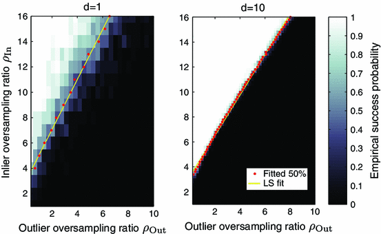
Exact subspace recovery with reaper. The heat maps show the empirical probability that reaper identifies a target subspace under the haystack model with varying inlier \(\rho _\mathrm{in}\) and outlier \(\rho _\mathrm{out}\) oversampling ratios. We perform the experiments in ambient dimension \(D=100\), with inlier dimension \(d=1\) (left) and \(d=10\) (right). For each value of \(\rho _\mathrm{in}\), we find the \(50\,\%\) empirical success \(\rho _\mathrm{out}\) (red dots). The yellow line indicates the least-squares fit to these points. In this parameter regime, a linear trend is clearly visible, which suggests that (3.1) captures the qualitative behavior of reaper under the haystack model (Color figure online)
In this experiment, \(N_{\mathrm{in}}\) increases in increments of 2 while \(N_{\mathrm{out}}\) increases in increments of \(20\).
More precisely, the inlier-to-outlier ratio must exceed \((121\mu /9) d \), where \(\mu \ge 1\) depends on the data.

References
Ammann, L.P.: Robust singular value decompositions: A new approach to projection pursuit. J. Amer. Statist. Assoc. 88(422), 505–514 (1993). http://www.jstor.org/stable/2290330
Bargiela, A., Hartley, J.K.: Orthogonal linear regression algorithm based on augmented matrix formulation. Comput. Oper. Res. 20, 829–836 (1993). doi:10.1016/0305-0548(93)90104-Q. http://dl.acm.org/citation.cfm?id=165819.165826
Basri, R., Jacobs, D.: Lambertian reflectance and linear subspaces. IEEE Trans. Pattern Anal. Mach. Intell. 25(2), 218–233 (2003)
Bhatia, R.: Matrix Analysis. No. 169 in Graduate Texts in Mathematics. Springer, New York (1997)
Björck, Å.: Numerical Methods for Least Squares Problems. Society for Industrial and Applied Mathematics, Philadelphia, PA (1996)
Bogachev, V.I.: Gaussian Measures, Mathematical Surveys and Monographs, vol. 62. American Mathematical Society, Providence, RI (1998)
Bonnans, J.F., Shapiro, A.: Perturbation Analysis of Optimization Problems. Springer Series in Operations Research. Springer (2000)
Boyd, S., Parikh, N., Chu, E., Peleato, B., Eckstein, J.: Distributed optimization and statistical learning via the alternating direction method of multipliers. Foundations and Trends in Machine Learning 3(1), 1–122 (2010). doi:10.1561/2200000016. http://www.nowpublishers.com/product.aspx?product=MAL&doi=2200000016
Brubaker, S.C.: Robust PCA and clustering in noisy mixtures. In: Proc. 20th Ann. ACM-SIAM Symp. Discrete Algorithms, SODA ’09, pp. 1078–1087. Society for Industrial and Applied Mathematics, Philadelphia, PA, USA (2009). http://portal.acm.org/citation.cfm?id=1496770.1496887
Caltech 101. Online (2006). http://www.vision.caltech.edu/Image_Datasets/Caltech101/
Candès, E.J., Li, X., Ma, Y., Wright, J.: Robust principal component analysis? J. Assoc. Comput. Mach. 58(3) (2011)
Cavalier, T.M., Melloy, B.J.: An iterative linear programming solution to the Euclidean regression model. Comput. Oper. Res. 18, 655–661 (1991)
Chan, T.F., Mulet, P.: On the convergence of the lagged diffusivity fixed point method in total variation image restoration. SIAM J. Numer. Anal. 36, 354–367 (1999). doi:10.1137/S0036142997327075
Chandrasekaran, V., Sanghavi, S., Parrilo, P.A., Willsky, A.S.: Rank-sparsity incoherence for matrix decomposition. SIAM J. Optim. 21(2), 572–596 (2011). doi:10.1137/090761793
Cook, R.D., Weisberg, S.: Residuals and influence in regression. Chapman and Hall, New York (1982)
Costeira, J., Kanade, T.: A multibody factorization method for independently moving objects. Int. J. Comput. Vision 29(3), 159–179 (1998)
Coudron, M., Lerman, G.: On the sample complexity of robust pca. In: NIPS, pp. 3230–3238 (2012)
Croux, C., Filzmoser, P., Oliveira, M.: Algorithms for projection pursuit robust principal component analysis. Chemometrics Intell. Lab. Sys. 87(2), 218–225 (2007)
Croux, C., Haesbroeck, G.: Principal component analysis based on robust estimators of the covariance or correlation matrix: Influence functions and efficiencies. Biometrika 87, 603–618 (2000)
Davidson, K.R., Szarek, S.J.: Local operator theory, random matrices and Banach spaces. In: Handbook of the geometry of Banach spaces, Vol. I, pp. 317–366. North-Holland, Amsterdam (2001). doi:10.1016/S1874-5849(01)80010-3
Davidson, K.R., Szarek, S.J.: Addenda and corrigenda to: “Local operator theory, random matrices and Banach spaces” [in Handbook of the geometry of Banach spaces, Vol. I, 317–366, North-Holland, Amsterdam, 2001; MR1863696 (2004f:47002a)]. In: Handbook of the geometry of Banach spaces, Vol. 2, pp. 1819–1820. North-Holland, Amsterdam (2003)
Davies, P.L.: Asymptotic behaviour of S-estimates of multivariate location parameters and dispersion matrices. Ann. Statist. 15(3), 1269–1292 (1987). http://www.jstor.org/stable/2241828
Deerwester, S., Dumais, S., Landauer, T., Furna, G., Beck, L.: Improving Information Retrieval with Latent Semantic Indexing. In: C.L. Borgman, E.Y.H. Pai (eds.) Information & Technology Planning for the Second 50 Years Proceedings of the 51st Annual Meeting of the American Society for Information Science, vol. 25. Learned Information Inc, Atlanta, Georgia (1988)
Devlin, S.J., Gnandesikan, R., Kettenring, J.R.: Robust estimation of dispersion matrices and principal components. J. Amer. Statist. Assoc. 76(374), 354–362 (1981). http://www.jstor.org/stable/2287836
Ding, C., Zhou, D., He, X., Zha, H.: R1-PCA: Rotational invariant \(L_1\)-norm principal component analysis for robust subspace factorization. In: ICML ’06: Proc. 23rd Int. Conf. Machine Learning, pp. 281–288. Association for Computing Machinery, Pittsburgh, PA (2006). doi:10.1145/1143844.1143880
Dodge, Y.: An introduction to \(l_1\)-norm based statistical data analysis. Comput. Statist. Data Anal. 5(4), 239–253 (1987). doi:10.1016/0167-9473(87)90048-X. http://www.sciencedirect.com/science/article/pii/016794738790048X
Eckart, C., Young, G.: A principal axis transformation for non-hermitian matrices. Bull. Amer. Math. Soc. 45(2), 118–121 (1939)
Epstein, R., Hallinan, P., Yuille, A.L.: \(5 \pm 2\) eigenimages suffice: An empirical investigation of low-dimensional lighting models. In: Physics-Based Modeling in Computer Vision, 1995, Proceedings of the Workshop on, p. 108 (1995). doi:10.1109/PBMCV.1995.514675
Eriksson, A., van den Hengel, A.: Efficient computation of robust low-rank matrix approximations in the presence of missing data using the \(l_1\) norm. In: Proc. 2010 IEEE Conf. Computer Vision and Pattern Recognition, pp. 771–778 (2010). doi:10.1109/CVPR.2010.5540139
Fei-Fei, L., Fergus, R., Perona, P.: Learning generative visual models from a few training examples: an incremental bayesian approach tested on 101 object categories. In: CVPR 2004, Workshop on Generative-Model Based Vision. IEEE (2004)
Fischler, M., Bolles, R.: Random sample consensus: A paradigm for model fitting with applications to image analysis and automated cartography. Comm. Assoc. Comput. Mach. 24(6), 381–395 (1981)
Goemans, M.X., Williamson, D.P.: Improved approximation for maximum cut and satisfiability problems using semidefinite programming. J. Assoc. Comput. Mach. 42, 1115–1145 (1995)
Grant, M., Boyd, S.: Graph implementations for nonsmooth convex programs. In: V. Blondel, S. Boyd, H. Kimura (eds.) Recent Advances in Learning and Control, Lecture Notes in Control and Information Sciences, pp. 95–110. Springer, London (2008). http://stanford.edu/~boyd/graph_dcp.html
Grant, M., Boyd, S.: CVX: Matlab software for disciplined convex programming, version 1.21. http://cvxr.com/cvx (2010)
Halko, N., Martinsson, P.G., Tropp, J.A.: Finding structure with randomness: Stochastic algorithms for constructing approximate matrix decompositions. SIAM Rev. 53(2), 217–288 (2011)
Harter, H.L.: The method of least squares and some alternatives: Part I. Int. Statist. Rev. 42(2), 147–174 (1974)
Harter, H.L.: The method of least squares and some alternatives: Part II. Int. Statist. Rev. 42(3), 235–282 (1974)
Ho, J., Yang, M., Lim, J., Lee, K., Kriegman, D.: Clustering appearances of objects under varying illumination conditions. In: Proc. 2003 IEEE Int. Conf. Computer Vision and Pattern Recognition, vol. 1, pp. 11–18 (2003)
Huber, P.J., Ronchetti, E.M.: Robust Statistics, 2nd edn. Wiley Series in Probability and Statistics. Wiley, Hoboken, NJ (2009). doi:10.1002/9780470434697
van Huffel, S., Vandewalle, J.: Total Least Squares: Computational Aspects and Analysis. Society for Industrial and Applied Mathematics, Philadelphia, PA (1987)
Jolliffe, I.T.: Principal Component Analysis, 2nd edn. Springer, Berlin (2002)
Kershaw, D.: Some extensions of W. Gautschi’s inequalities for the gamma function. Math. Comput. 41(164), pp. 607–611 (1983). http://www.jstor.org/stable/2007697
Kwak, N.: Principal component analysis based on \(L_1\)-norm maximization. IEEE Trans. Pattern Anal. Mach. Intell. 30(9), 1672–1680 (2008). doi:10.1109/TPAMI.2008.114
Ledoux, M., Talagrand, M.: Probability in Banach spaces, Ergebnisse der Mathematik und ihrer Grenzgebiete (3) [Results in Mathematics and Related Areas (3)], vol. 23. Springer, Berlin (1991). Isoperimetry and processes
Lee, K.C., Ho, J., Kriegman, D.: Acquiring linear subspaces for face recognition under variable lighting. IEEE Trans. Pattern Anal. Mach. Intell. 27(5), 684–698 (2005)
Lerman, G., McCoy, M.B., Tropp, J.A., Zhang, T.: Robust computation of linear models, or how to find a needle in a haystack (2012). Available at arxiv:1202.4044v1
Lerman, G., Zhang, T.: \(\ell _p\)-Recovery of the most significant subspace among multiple subspaces with outliers. Constr. Approx. (2014). doi:10.1007/s00365-014-9242-6
Lerman, G., Zhang, T.: Robust recovery of multiple subspaces by geometric \(\ell _p\) minimization. Ann. Statist. 39(5), 2686–2715 (2011)
Li, G., Chen, Z.: Projection-pursuit approach to robust dispersion matrices and principal components: Primary theory and Monte Carlo. J. Amer. Statist. Assoc. 80(391), 759–766 (1985). doi:10.2307/2288497
Liu, G., Lin, Z., Yan, S., Sun, J., Yu, Y., Ma, Y.: Robust recovery of subspace structures by low-rank representation. IEEE Trans. Pattern Anal. Mach. Intell. 35(1), 171–184 (2013). doi:10.1109/TPAMI.2012.88
Locantore, N., Marron, J.S., Simpson, D.G., Tripoli, N., Zhang, J.T., Cohen, K.L.: Robust principal component analysis for functional data. Test 8(1), 1–73 (1999). doi:10.1007/BF02595862. With discussion and a rejoinder by the authors
Lovasz, L., Schrijver, A.: Cones of matrices and set-functions and 0-1 optimization. SIAM J. Optim. 1(2), 166–190 (1991). doi:10.1137/0801013. http://link.aip.org/link/?SJE/1/166/1
Maronna, R.: Principal components and orthogonal regression based on robust scales. Technometrics 47(3), 264–273 (2005). doi:10.1198/004017005000000166
Maronna, R.A.: Robust M-estimators of multivariate location and scatter. Ann. Statist. 4(1), 51–67 (1976). http://www.jstor.org/stable/2957994
Maronna, R.A., Martin, D.R., Yohai, V.J.: Robust Statistics. Wiley Series in Probability and Statistics. Wiley, Chichester (2006). doi:10.1002/0470010940. Theory and methods
McCoy, M., Tropp, J.A.: Two proposals for robust PCA using semidefinite programming. Electron. J. Statist. 5, 1123–1160 (2011)
Novembre, J., Johnson, T., Bryc, K., Kutalik, Z., Boyko, A.R., Auton, A., Indap, A., King, K.S., Bergmann, S., Nelson, M., Stephens, M., Bustamante, C.D.: Genes mirror geography within Europe. Nature 456(7218), 98–101 (2008). doi:10.1038/nature07331. http://www.ncbi.nlm.nih.gov/pubmed/18758442?itool=EntrezSystem2.PEntrez.Pubmed.Pubmed_ResultsPanel.Pubmed_RVDocSum&ordinalpos=8
Nyquist, H.: Least orthogonal absolute deviations. Comput. Statist. Data Anal. 6(4), 361–367 (1988). doi:10.1016/0167-9473(88)90076-X. http://www.sciencedirect.com/science/article/pii/016794738890076X
Osborne, M.R., Watson, G.A.: An analysis of the total approximation problem in separable norms, and an algorithm for the total \(l_1 \) problem. SIAM J. Sci. Statist. Comput. 6(2), 410–424 (1985). doi:10.1137/0906029. http://link.aip.org/link/?SCE/6/410/1
Overton, M.L., Womersley, R.S.: On the sum of the largest eigenvalues of a symmetric matrix. SIAM J. Matrix Anal. Appl. 13(1), 41–45 (1992)
Price, A.L., Patterson, N.J., Plenge, R.M., Weinblatt, M.E., Shadick, N.A., Reich, D.: Principal components analysis corrects for stratification in genome-wide association studies. Nature Genetics 38(8), 904–909 (2006). http://www.ncbi.nlm.nih.gov/pubmed/16862161
Rockafellar, R.T.: Convex analysis. Princeton Mathematical Series, No. 28. Princeton University Press, Princeton, N.J. (1970)
Rousseeuw, P.J.: Least median of squares regression. J. Amer. Statist. Assoc. 79(388), 871–880 (1984)
Rousseeuw, P.J., Leroy, A.M.: Robust Regression and Outlier Detection. Wiley Series in Probability and Mathematical Statistics: Applied Probability and Statistics. Wiley, New York (1987)
Späth, H., Watson, G.A.: On orthogonal linear approximation. Numer. Math. 51, 531–543 (1987). doi:10.1007/BF01400354. http://dl.acm.org/citation.cfm?id=34311.34315
Torre, F.D.L., Black, M.J.: Robust principal component analysis for computer vision. In: Proc. 8th IEEE Conf. Computer Vision, vol. 1, pp. 362–369 vol. 1 (2001). doi:10.1109/ICCV.2001.937541
Torre, F.D.L., Black, M.J.: A framework for robust subspace learning. Int. J. Comput. Vision 54, 117–142 (2003). doi:10.1023/A:1023709501986
Tropp, J.A.: Just relax: convex programming methods for identifying sparse signals in noise. IEEE Trans. Inform. Theory 52(3), 1030–1051 (2006). doi:10.1109/TIT.2005.864420
Tropp, J.A.: Corrigendum in “just relax: Convex programming methods for identifying sparse signals in noise”. IEEE Trans. Inform. Theory 55(2) (2009)
Vazirani, V.V.: Approximation Algorithms. Springer, Berlin (2003)
Voss, H., Eckhardt, U.: Linear convergence of generalized Weiszfeld’s method. Computing 25, 243–251 (1980). doi:10.1007/BF02242002
Wang, L., Singer, A.: Exact and stable recovery of rotations for robust synchronization. Information and Inference (2013). doi:10.1093/imaiai/iat005
Watson, G.A.: Some problems in orthogonal distance and non-orthogonal distance regression. In: Proc. 2001 Symp. Algorithms for Approximation IV. Defense Technical Information Center (2001). http://books.google.com/books?id=WKKWGwAACAAJ
Watson, G.A.: On the Gauss-Newton method for \(l_1\) orthogonal distance regression. IMA J. Numer. Anal. 22(3), 345–357 (2002). doi:10.1093/imanum/22.3.345. http://imajna.oxfordjournals.org/content/22/3/345.abstract
Witten, D., Tibshirani, R., Hastie, T.: A penalized matrix decomposition, with applications to sparse principal components and canonical correlation analysis. Biostat. 10(3), 515–534 (2009)
Xu, H., Caramanis, C., Mannor, S.: Principal Component Analysis with Contaminated Data: The High Dimensional Case. In: Proc. 2010 Conf. Learning Theory. OmniPress, Haifa (2010)
Xu, H., Caramanis, C., Sanghavi, S.: Robust PCA via outlier pursuit. In: J. Lafferty, C.K.I. Williams, J. Shawe-Taylor, R. Zemel, A. Culotta (eds.) Neural Information Processing Systems 23, pp. 2496–2504. MIT Press, Vancouver (2010)
Xu, H., Caramanis, C., Sanghavi, S.: Robust PCA via outlier pursuit. IEEE Trans. Inform. Theory 58(5), 3047–3064 (2012)
Xu, L., Yuille, A.L.: Robust principal component analysis by self-organizing rules based on statistical physics approach. IEEE Trans. Neural Networks 6(1), 131–143 (1995). doi:10.1109/72.363442
Xu, L., Yuille, A.L.: Robust principal component analysis by self-organizing rules based on statistical physics approach. IEEE Trans. Neural Networks 6(1), 131–143 (1995). doi:10.1109/72.363442
Zhang, T., Szlam, A., Lerman, G.: Median \(K\)-flats for hybrid linear modeling with many outliers. In: Proc. 12th IEEE Int. Conf. Computer Vision, pp. 234–241. Kyoto (2009). doi:10.1109/ICCVW.2009.5457695
Acknowledgments
Lerman and Zhang were supported in part by the IMA and by NSF Grants DMS-09-15064 and DMS-09-56072. McCoy and Tropp were supported by Office of Naval Research (ONR) Awards N00014-08-1-0883 and N00014-11-1002, Air Force Office of Scientific Research (AFOSR) Award FA9550-09-1-0643, Defense Advanced Research Projects Agency (DARPA) Award N66001-08-1-2065, and a Sloan Research Fellowship. The authors thank Eran Halperin, Yi Ma, Ben Recht, Amit Singer, and John Wright for helpful conversations. The anonymous referees provided many thoughtful and incisive remarks that helped us improve the manuscript immensely.
Author information
Authors and Affiliations
Corresponding author
Additional information
Communicated by Emmanuel Candès.
Appendices
Appendix 1: Theorem 2.1: Supporting Lemmas
This appendix contains the proofs of the two technical results that animate Theorem 2.1. Throughout, we maintain the notation and assumptions from the In & Out model on p. 6 and from the statement and proof of Theorem 2.1.
1.1 Controlling the Size of the Perturbation
In this section, we establish Lemma 2.2. On comparing the objective function \(f\) from (2.6) with the perturbed objective function \(g\) from (2.9), we see that the only changes involve the terms containing inliers. As a consequence, the difference function \(h = f - g\) depends only on the inliers:
where \(\varvec{P}\) is an arbitrary matrix. Apply the lower triangle inequality to see that
To justify the second inequality, write \(\mathbf {I}- \varvec{P} = (\mathbf {I}- \varvec{\varPi }_{L}) + (\varvec{\varPi }_{L} - \varvec{P})\), and then apply the upper triangle inequality. Use the fact that the projector \(\mathbf {I}- \varvec{\varPi }_{L}\) is idempotent to simplify the resulting expression. The third inequality depends on the usual operator-norm bound. We reach (7.1) by identifying the sum as the total inlier residual \(\fancyscript{R}(L)\), defined in (2.2), and invoking the fact that the Schatten 1-norm dominates the operator norm.
Applying (7.1) twice, it becomes apparent that
There are no restrictions on the matrix \(\varvec{\varDelta }\), so the demonstration of Lemma 2.2 is complete.
1.2 Rate of Ascent of Perturbed Objective
In this section, we establish Lemma 2.3. This result contains the essential insights behind Theorem 2.1, and the proof involves some amount of exertion.
Assume that \(\varvec{\varPi }_{L} + \varvec{\varDelta } \in \varPhi \). Since the perturbed objective \(g\) defined in (2.9) is a continuous convex function, we have the lower bound
The right-hand side of (7.2) refers to the one-sided directional derivative of \(g\) at the point \(\varvec{\varPi }_{L}\) in the direction \(\varvec{\varDelta }\). That is,
We can be confident that this limit exists and takes a finite value [62, Theorem 23.1 et seq.].
Let us find a practicable expression for the directional derivative. Recalling the definition (2.9) of the perturbed objective, we see that the difference quotient takes the form
We analyze the two sums separately. First, consider the terms that involve inliers. For \(\varvec{x} \in \fancyscript{X}_{\mathrm{in}}\),
We have used the fact that \(\varvec{\varPi }_{L^\perp } \varvec{\varPi }_L = \varvec{0}\) twice. Next, consider the terms involving outliers. By the assumptions of the In & Out model on p. 6, each outlier \(\varvec{x} \in \fancyscript{X}_{\mathrm{out}}\) has a nontrivial component in the subspace \(L^{\perp }\). We may calculate that
where the spherization transform \(\varvec{x} \mapsto \widetilde{\varvec{x}}\) is defined in (1.1). Therefore,
Introducing these facts into the difference quotient (7.3) and taking the limit as \(t \downarrow 0\), we determine that
It remains to produce a lower bound on this directional derivative.
The proof of the lower bound has two components. We require a bound on the sum over outliers, and we require a bound on the sum over inliers. These results appear in the following sublemmas, which we prove in Sects. 7.2.1 and 7.2.2.
Sublema 7.1
(Outliers) Under the prevailing assumptions,
where the alignment statistic \(\fancyscript{A}(L)\) is defined in (2.3).
Sublema 7.2
(Inliers) Under the prevailing assumptions,
where the permeance statistic \(\fancyscript{P}(L)\) is defined in (2.1).
To complete the proof of Lemma 2.3, we substitute the bounds from Sublemmas 7.1 and 7.2 into the expression (7.4) for the directional derivative. This step yields
Since \(d = \dim (L)\), we identify the bracket as the stability statistic \(\fancyscript{S}(L)\) defined in (2.4). Combine this bound with (7.2) to complete the argument.
1.2.1 Outliers
The result in Sublemma 7.1 is straightforward. First, observe that
The first relation follows from the fact that \(\left\langle {\varvec{A}\varvec{b}},\ {\varvec{c}} \right\rangle = \left\langle { \varvec{A} },\ {\varvec{c}\varvec{b}^\mathsf{t}} \right\rangle \). We obtain the second identity by drawing the sum into the inner product and recognizing the product of the two matrices. Therefore,
The last bound is an immediate consequence of the duality between the spectral norm and the Schatten 1-norm. To complete the argument, we apply the operator norm bound \(\left\| {\varvec{AB}^\mathsf{t}} \right\| \le \left\| {\varvec{A}} \right\| \left\| {\varvec{B}} \right\| \).
1.2.2 Inliers
The proof of Sublemma 7.2 involves several considerations. We first explain the overall structure of the argument and then verify that each part is correct. The first ingredient is a lower bound for the minimum of the sum over inliers:
(Sect. 7.2.3). The second step depends on a simple comparison between the Frobenius norm and the Schatten 1-norm of a matrix:
The inequality (7.6) follows immediately when we express the two norms in terms of singular values and apply the fact that \(\varvec{\varDelta } \varvec{\varPi }_{L}\) has rank \(d\); it requires no further comment. Third, we argue that
This demonstration appears in Sect. 7.2.4. Combining the bounds (7.5), (7.6), and (7.7), we obtain the result stated in Sublemma 7.2
1.2.3 Minimization with a Frobenius-Norm Constraint
To establish (7.5), we assume that \(\left\| { \varvec{\varDelta } \varvec{\varPi }_{L} } \right\| _{\mathrm{F}} = 1\). The general case follows from homogeneity.
Let us introduce a (thin) SVD \(\varvec{\varDelta }\varvec{\varPi }_{L} = \varvec{U\varSigma V}^\mathsf{t}\). Observe that each column \(\varvec{v}_1, \dots , \varvec{v}_d\) of the matrix \(\varvec{V}\) is contained in \(L\). In addition, the singular values \(\sigma _j\) satisfy \(\sum _{j=1}^d \sigma _j^2 = 1\) because of the normalization of the matrix.
We can express the quantity of interest as
The first identity follows from the unitary invariance of the Euclidean norm. In the second relation, we have just written out the Euclidean norm in detail. To facilitate the next step, abbreviate \(p_j = \sigma _j^2\) for each index \(j\). Calculate that
Indeed, the right-hand side of the first line is a concave function of the variables \(p_j\). By construction, these variables lie in the convex set determined by the constraints \(p_j \ge 0\) and \(\sum _j p_j = 1\). The minimizer of a concave function over a convex set occurs at an extreme point, which delivers the first inequality. To reach the last inequality, recall that each \(\varvec{v}_j\) is a unit vector in \(L\). This expression implies (7.5).
1.2.4 Feasible Directions
Finally, we need to verify the relation (7.7), which states that \(\left\| {\varvec{\varDelta } \varvec{\varPi }_{L}} \right\| _{S_1}\) is comparable to \(\left\| {\varvec{\varDelta }} \right\| _{S_1}\), provided that \(\varvec{\varPi }_{L} + \varvec{\varDelta } \in \varPhi \). To that end, we decompose the matrix \(\varvec{\varDelta }\) into blocks:
We claim that
Given identity (7.9), we can establish the equivalence of norms promised in (7.7). Indeed,
The first inequality holds because projection reduces the Schatten 1-norm of a matrix. The second inequality is numerical. The equality in the third line depends on the claim (7.9). The last bound follows from the subadditivity of the norm and (7.8).
To check (7.9), we recall the definition of the feasible set:
The condition \(\varvec{\varPi }_L + \varvec{\varDelta } \in \varPhi \) implies the semidefinite relation \(\varvec{\varPi }_{L} + \varvec{\varDelta } \preccurlyeq \mathbf {I}\). Conjugating by the orthoprojector \(\varvec{\varPi }_{L}\), we see that
As a consequence, \(\varvec{\varDelta }_1 \preccurlyeq \varvec{0}\). Similarly, the relation \(\varvec{0} \preccurlyeq \varvec{\varPi }_L + \varvec{\varDelta }\) yields
Therefore, \(\varvec{\varDelta }_3 \succcurlyeq \varvec{0}\). Since \(\mathrm{tr }(\varvec{\varPi }_L + \varvec{\varDelta }) = d\) and \(\mathrm{tr }\,\varvec{\varPi }_{L} = d\), it is clear that \(0 = \mathrm{tr }\,\varvec{\varDelta } = \mathrm{tr }(\varvec{\varDelta }_1 + \varvec{\varDelta }_3)\). We conclude that
The first and third equalities hold because the Schatten 1-norm of a positive-semidefinite matrix coincides with its trace.
Appendix 2: Analysis of Haystack Model
In this appendix, we establish exact recovery conditions for the haystack model. To accomplish this goal, we study the probabilistic behavior of the permeance statistic and the alignment statistic. Our main result for the haystack model, Theorem 8.1, follows when we introduce the probability bounds into the deterministic recovery result, Theorem 2.1. The simplified result for the haystack model, Theorem 3.1, is a consequence of the following more detailed theory.
Theorem 8.1
Fix a parameter \(c > 0\). Let \(L\) be an arbitrary \(d\)-dimensional subspace of \(\mathbb {R}^D\), and draw the data set \(\fancyscript{X}\) at random according to the haystack model on p. 11. Let \(1 \le d \le D-1\). The stability statistic satisfies
except with probability \(3.5 \, \mathrm{e}^{-c^2 d /2}\).
We verify this expression subsequently in Sects. 8.1 and 8.2. For now, we demonstrate that Theorem 8.1 contains the simplified result for the haystack model, Theorem 3.1.
Proof of Theorem 3.1 from Theorem 8.1
To begin, we collect some numerical inequalities. For \(\alpha >0\), the function \(f(x) = x - \alpha \sqrt{x}\) is convex when \(x \ge 0\), so that
For \(1 \le d \le (D-1)/2\), we have the numerical bounds
Finally, recall that \((a+b)^2 \le 2(a^2 + b^2)\) and \((a+b+e)^2 \le 3(a^2+b^2+e^2)\) as a consequence of Hölder’s inequality.
To prove Theorem 3.1, we apply our numerical inequalities to weaken the bound (8.1) from Theorem 8.1 to
Set \(c = \sqrt{2 \beta }\) to reach the conclusion. \(\square \)
1.1 Tools for Computing the Summary Statistics
The proof of Theorem 8.1 requires probability bounds on the permeance statistic \(\fancyscript{P}\) and the alignment statistic \(\fancyscript{A}\). These bounds follow from tail inequalities for Gaussian and spherically distributed random vectors that we develop in the next two subsections.
1.1.1 Tools for Permeance Statistic
In this section, we develop the probability inequality that we need to estimate the permeance statistic \(\fancyscript{P}(L)\) for data drawn from the haystack model.
Lemma 8.2
Suppose \(\varvec{g}_1, \dots , \varvec{g}_n\) are i.i.d. \(\textsc {normal}(\varvec{0}, \mathbf {I})\) vectors in \(\mathbb {R}^d\). For each \(t \ge 0\),
except with probability \(\mathrm{e}^{-t^2/2}\).
Proof
Add and subtract the mean from each summand on the left-hand side of (8.2) to obtain
The second sum on the right-hand side has a closed-form expression because each term is the expectation of a half-Gaussian random variable: \(\mathrm{\mathbb {E} }\left| {\left\langle {\varvec{u}},\ {\varvec{g}_i} \right\rangle } \right| = \sqrt{2/\pi }\) for every unit vector \(\varvec{u}\). Therefore,
To control the first sum on the right-hand side of (8.3), we use a standard argument. To bound the mean, we symmetrize the sum and invoke a comparison theorem. To control the probability of a large deviation, we apply a measure concentration argument.
To proceed with the calculation of the mean, we use the Rademacher symmetrization lemma [44, Lemma 6.3] to obtain
The random variables \(\varepsilon _1, \dots , \varepsilon _n\) are i.i.d. Rademacher random variables that are independent of the Gaussian sequence. Next, invoke the Rademacher comparison theorem [44, Eq. (4.20)] with the function \(\phi (\cdot ) = \left| {\cdot } \right| \) to obtain the further bound
The identity follows when we draw the sum into the inner product to maximize over all unit vectors. From here, the rest of the argument is very easy. Use Jensen’s inequality to bound the expectation by the root mean square, which has a closed form:
Note that the mean fluctuation (8.5) is dominated by the centering term (8.4) when \(n \gg d\).
To control the probability that the fluctuation term is large, we use a standard concentration inequality [6, Theorem 1.7.6] for a Lipschitz function of independent Gaussian variables. Define a real-valued function on \(d \times n\) matrices: \( f(\varvec{Z}) = \sup _{\left\| {\varvec{u}} \right\| = 1} \ \sum _{i=1}^n ( \sqrt{2/\pi } - \left| {\left\langle {\varvec{u}},\ {\varvec{z}_i} \right\rangle } \right| ), \) where \(\varvec{z}_i\) denotes the \(i\)th column of \(\varvec{Z}\). Compute that
Therefore, \(f\) has Lipschitz constant \(\sqrt{n}\) with respect to the Frobenius norm. In view of the estimate (8.5) for the mean, the Gaussian concentration bound implies that
Introduce the bound (8.6) and the identity (8.4) into (8.3) to complete the proof. \(\square \)
1.1.2 Tools for Alignment Statistic
In this section, we develop the probability inequalities that we need to estimate the alignment statistic \(\fancyscript{A}(L)\) for data drawn from the haystack model. First, we need a tail bound for the maximum singular value of a Gaussian matrix. The following inequality is a well-known consequence of Slepian’s lemma. See [20, Theorem 2.13] and the errata [21] for details.
Proposition 8.3
Let \(\varvec{G}\) be an \(m \times n\) matrix whose entries are i.i.d. standard normal random variables. For each \(t \ge 0\),
where \(\varPhi (t)\) is the Gaussian cumulative density function
We also need a related result for random matrices with independent columns that are uniformly distributed on the sphere. The argument bootstraps from Proposition 8.3.
Lemma 8.4
Let \(\varvec{S}\) be an \(m \times n\) matrix whose columns are i.i.d. random vectors distributed uniformly on the sphere \(\mathbb {S}^{m-1}\) in \(\mathbb {R}^m\). For each \(t \ge 0\),
Proof
Fix \(\theta > 0\). The Laplace transform method shows that
We compare \(\left\| {\varvec{S}} \right\| \) with the norm of a Gaussian matrix by introducing a diagonal matrix of \(\chi \)-distributed variables. The rest of the argument is purely technical.
Let \(\varvec{r} = (r_1, \dots , r_n)\) be a vector of i.i.d. \(\chi \)-distributed random variables with \(m\) degrees of freedom. Recall that \(r_i \, \widetilde{\varvec{g}}_i \sim \varvec{g}_i\), where \(\widetilde{\varvec{g}}_i\) is uniform on the sphere and \(\varvec{g}_i\) is standard normal. The mean of a \(\chi \)-distributed variable satisfies an inequality due to Kershaw [42]:
Using Kershaw’s bound and Jensen’s inequality, we obtain
where \(\varvec{G}\) is an \(m \times n\) matrix with i.i.d. standard normal entries.
Define a random variable \(Z := \left\| {\varvec{G}} \right\| - \sqrt{n} - \sqrt{m}\), and let \(Z_+ := \max \{Z, 0\}\) denote its positive part. Then
Apply the cumulative density function bound in Proposition 8.3, and identify the complementary error function \(\mathrm{erfc }\):
A computer algebra system will report that this frightening integral has a closed form:
We have used the simple bound \(\mathrm{erf }(\theta ) \le 1\) for \(\theta \ge 0\). In summary,
Select \(\theta = t\) to obtain the advertised bound (8.7). \(\square \)
1.2 Proof of Theorem 8.1
Suppose that the data set \(\fancyscript{X}\) is drawn from the haystack model on p. 11. Let \(\varvec{X}_{\mathrm{out}}\) be a \(D \times N_{\mathrm{out}}\) matrix whose columns are the outliers \(\varvec{x} \in \fancyscript{X}_{\mathrm{out}}\), arranged in fixed order. Recall the inlier sampling ratio \(\rho _{\mathrm{in}} := N_{\mathrm{in}} / d\) and the outlier sampling ratio \(\rho _{\mathrm{out}} := N_{\mathrm{out}}/D\).
Let us begin with a lower bound for the permeance statistic \(\fancyscript{P}(L)\). The \(N_{\mathrm{in}}\) inliers are drawn from a centered Gaussian distribution on the \(d\)-dimensional space \(L\) with covariance \((\sigma _{\mathrm{in}}^2 / d) \, \mathbf {I}_L\). Rotational invariance and Lemma 8.2, with \(t = c\sqrt{d}\), together imply that the permeance statistic (2.1) satisfies
except with probability \(\mathrm{e}^{-c^2 d/2}\).
Next, we obtain an upper bound for the alignment statistic \(\fancyscript{A}(L)\). The \(N_{\mathrm{out}}\) outliers are independent, centered Gaussian vectors in \(\mathbb {R}^D\) with covariance \((\sigma _\mathrm{out}^2 / D) \, \mathbf {I}\). Proposition 8.3, with \(t = c\sqrt{d}\), shows that
except with probability \(\mathrm{e}^{-c^2 d/2}\). Rotational invariance implies that the columns of \(\widetilde{ \varvec{\varPi }_{L^\perp } \varvec{X}_{\mathrm{out}} }\) are independent vectors that are uniformly distributed on the unit sphere of a \((D-d)\)-dimensional space. Lemma 8.4 yields
except with probability \(1.5 \, \mathrm{e}^{-c^2 d / 2}\). It follows that
except with probability \(2.5 \, \mathrm{e}^{-c^2 d/ 2}\).
Combining these bounds, we discover that the stability statistic satisfies
except with probability \(3.5 \, \mathrm{e}^{-c^2 d / 2}\). This completes the argument.
Appendix 3: Analysis of IRLS Algorithm
This appendix contains the details of our analysis of the IRLS method, Algorithm 4.2. First, we verify that Algorithm 4.1 reliably solves the weighted least-squares subproblem (4.1). Then we argue that IRLS converges to a point near the true optimum of the reaper problem (1.4).
1.1 Solving the Weighted Least-Squares Problem
In this section, we verify that Algorithm 4.1 correctly solves the weighted least-squares problem (4.1). The following lemma provides a more mathematical statement of the algorithm, along with the proof of correctness. Note that this statement is slightly more general than the recipe presented in Algorithm 4.1 because it is valid over the entire range \(0<d<D\).
Lemma 9.1
(Solving the Weighted Least-Squares Problem) Assume that \(0 < d < D\), and suppose that \(\fancyscript{X}\) is a set of observations in \(\mathbb {R}^D\). For each \(\varvec{x} \in \fancyscript{X}\), let \(\beta _{\varvec{x}}\) be a nonnegative weight. Form the weighted sample covariance matrix \(\varvec{C}\), and compute its eigenvalue decomposition:
When \(\mathrm{rank }(\varvec{C}) \le d\), construct a vector \(\varvec{\nu } \in \mathbb {R}^D\) via the formula
When \(\mathrm{rank }(\varvec{C}) > d\), define the positive quantity \(\theta \) implicitly by solving the equation
Construct a vector \(\varvec{\nu } \in \mathbb {R}^D\) whose components are
In either case, an optimal solution to (4.1) is given by
In this statement, we enforce the convention \(0/0 := 0\), and \(\mathrm{diag }\) forms a diagonal matrix from a vector.
Proof of Lemma 9.1
First, observe that the construction (9.4) yields a matrix \(\varvec{P}_{\star }\) that satisfies the constraints of (4.1) in both cases.
When \(\mathrm{rank }(\varvec{C}) \le d\), we can verify that our construction of the vector \(\varvec{\nu }\) yields an optimizer of (4.1) by showing that the objective value is zero, which is minimal. Evaluate the objective function (4.1) at the point \(\varvec{P}_{\star }\) to see that
by the definition of \(\varvec{C}\) and the fact that \(\varvec{C}\) and \(\varvec{P}_{\star }\) are simultaneously diagonalizable. The nonzero eigenvalues of \(\varvec{C}\) appear among \(\lambda _1, \ldots , \lambda _{\lfloor d \rfloor }\). At the same time, \(1 - \nu _i = 0\) for each \(i = 1, \ldots , \lfloor d \rfloor \). Therefore, the value of (9.5) equals zero at \(\varvec{P}_{\star }\).
Next, assume that \(\mathrm{rank }(\varvec{C}) > d\). The objective function in (4.1) is convex, so we can verify that \(\varvec{P}_{\star }\) solves the optimization problem if the directional derivative of the objective at \(\varvec{P}_{\star }\) is nonnegative in every feasible direction. A matrix \(\varvec{\varDelta }\) is a feasible perturbation if and only if
Let \(\varvec{\varDelta }\) be an arbitrary matrix that satisfies these constraints. By expanding the objective of (4.1) about \(\varvec{P}_{\star }\), easily compute the derivative in the direction \(\varvec{\varDelta }\). In particular, the condition
ensures that the derivative increases in the direction \(\varvec{\varDelta }\). We now set about verifying (9.6) for our choice of \(\varvec{P}_\star \) and all feasible \(\varvec{\varDelta }\).
Note first that the quantity \(\theta \) can be defined. Indeed, the left-hand side of (9.2) equals \(\mathrm{rank }(\varvec{C})\) when \(\theta = 0\), and it equals zero when \(\theta \ge \lambda _1\). By continuity, there exists a value of \(\theta \) that solves the equation. Let \(i_{\star }\) be the largest index where \(\lambda _{i_{\star }} > \theta \), so that \(\nu _{i} = 0\) for each \(i > i_{\star }\). Next, define \(M\) as the subspace spanned by the eigenvectors \(\varvec{u}_{i_{\star } + 1}, \dots , \varvec{u}_D\). Since \(\nu _i\) is the eigenvalue of \(\varvec{P}_{\star }\) with eigenvector \(\varvec{u}_i\), we must have \(\varvec{\varPi }_{M} \varvec{P}_{\star } \varvec{\varPi }_M = \varvec{0}\). It follows that \(\varvec{\varPi }_M \varvec{\varDelta } \varvec{\varPi }_M \succcurlyeq \varvec{0}\) because \(\varvec{\varPi }_M (\varvec{P}_{\star } + \varvec{\varDelta }) \varvec{\varPi }_M \succcurlyeq \varvec{0}\).
To complete the argument, observe that
Therefore, \((\mathbf {I}- \varvec{P}_{\star }) \varvec{C} = \varvec{U} \cdot \mathrm{diag }( \min \{ \lambda _i, \theta \} ) \cdot \varvec{U}^\mathsf{t}\). Using the fact that \(\mathrm{tr }\,\varvec{\varDelta } = 0\), we obtain
Since \(\lambda _i \le \theta \) for each \(i > i_{\star }\), each eigenvalue of \(\varvec{Z}\) is nonpositive. Furthermore, \(\varvec{\varPi }_M \varvec{Z} \varvec{\varPi }_M = \varvec{Z}\). We see that
because the compression of \(\varvec{\varDelta }\) on \(M\) is positive semidefinite and \(\varvec{Z}\) is negative semidefinite. In other words, (9.6) is satisfied for every feasible perturbation \(\varvec{\varDelta }\) about \(\varvec{P}_{\star }\). \(\square \)
1.2 Convergence of IRLS
In this section, we argue that the IRLS method of Algorithm 4.2 converges to a point whose value is nearly optimal for the reaper problem (1.4). The proof consists of two phases. First, we explain how to modify the argument from [13] to show that the iterates \(\varvec{P}^{(k)}\) converge to a matrix \(\varvec{P}_\delta \), which is characterized as the solution to a regularized counterpart of reaper. The fact that the limit point \(\varvec{P}_\delta \) achieves a near-optimal value for reaper follows from the characterization.
Proof sketch for Theorem 4.1
We find it more convenient to work with the variables \(\varvec{Q} := \mathbf {I}-\varvec{P}\) and \(\varvec{Q}^{(k)} := \mathbf {I}-\varvec{P}^{(k)}\). First, let us define a regularized objective. For a parameter \(\delta > 0\), consider the Huber-like function
We introduce the convex function
The second identity above highlights the interpretation of \(F\) as a regularized objective function for (1.4) under the assignment \(\varvec{Q} = \mathbf {I}-\varvec{P}\). Note that \(F\) is continuously differentiable at each matrix \(\varvec{Q}\), and the gradient
The technical assumption that the observations do not lie in the union of two strict subspaces of \(\mathbb {R}^D\) implies that \(F\) is strictly convex; compare with the proof of [80, Theorem 2]. We define \(\varvec{Q}_{\delta }\) as the solution of a constrained optimization problem:
The strict convexity of \(F\) implies that \(\varvec{Q}_{\delta }\) is well defined.
The key idea in the proof is to show that the iterates \(\varvec{Q}^{(k)}\) of Algorithm 4.2 converge to the optimizer \(\varvec{Q}_\delta \) of the regularized objective function \(F\). We demonstrate that Algorithm 4.2 is a generalized Weiszfeld method in the sense of [13, Sect. 4]. After defining some additional auxiliary functions and facts about these functions, we explain how the argument of [13, Lem. 5.1] can be adapted to prove that the iterates of \(\varvec{Q}^{(k)}=\mathbf {I}-\varvec{P}^{(k)}\rightarrow \varvec{Q}_\delta \). The only innovation required is an inequality from convex analysis that lets us handle the constraints \(\varvec{0} \preccurlyeq \varvec{Q} \preccurlyeq \mathbf {I}\) and \(\mathrm{tr }\,\varvec{Q} = D-d\).
Now for the definitions. We introduce the potential function
Then \(G(\cdot ,\ \varvec{Q}^{(k)})\) is a smooth quadratic function. By collecting terms, we may relate \(G\) and \(F\) through the expansion
where \(C\) is the continuous function
Next, we verify some facts related to Hypotheses 4.2 and 4.3 of [13, Sect. 4]. Note that \(F(\varvec{Q})= G(\varvec{Q},\ \varvec{Q})\). Furthermore, \(F(\varvec{Q}) \le G(\varvec{Q},\ \varvec{Q}^{(k)})\) because \(H_\delta (x, x) \le H_\delta (x,y)\), which is a direct consequence of the arithmetic-geometric mean inequality.
We now relate the iterates of Algorithm 4.2 to the definitions given earlier. Given that \(\varvec{Q}^{(k)} = \mathbf {I}-\varvec{P}^{(k)}\), Step 2b of Algorithm 4.2 is equivalent to the iteration
From this characterization we have the monotonicity property
This fact motivates the stopping criterion for Algorithm 4.2 because it implies the objective values are decreasing: \( \alpha ^{(k+1)} = F(\varvec{Q}^{k+1}) \le F(\varvec{Q}^{(k)}) = \alpha ^{(k)}\).
We also require some information regarding the bilinear form induced by \(C\). Introduce the quantity \(m := \max \left\{ \delta , \ \max _{\varvec{x} \in \fancyscript{X}}\{ \left\| {\varvec{x}} \right\| \}\right\} \). Then, by the symmetry of the matrix \(\varvec{Q}\) and the fact that the inner product between positive semidefinite matrices is nonnegative, we have
The technical assumption that the observations do not lie in two strict subspaces of \(\mathbb {R}^D\) implies in particular that the observations span \(\mathbb {R}^D\). We deduce that \(\mu >0\).
Now we discuss the challenge imposed by the constraint set. When the minimizer \(\varvec{Q}^{(k+1)}\) lies on the boundary of the constraint set, the equality [13, Eq. (4.3)] may not hold. However, if we denote the gradient of \(G\) with respect to its first argument by \(G_{\varvec{Q}}\), the inequality
holds for every \(\varvec{Q}\) in the feasible set. This is simply the first-order necessary and sufficient condition for the constrained minimum of a smooth convex function over a convex set.
With the aforementioned facts, a proof that the iterates \(\varvec{Q}^{(k)}\) converge to \(\varvec{Q}_\delta \) follows the argument of [13, Lemma 5.1] nearly line by line. However, due to inequality (9.8), the final conclusion is that, at the limit point \(\overline{\varvec{Q}}\), the inequality \(\left\langle {\varvec{Q} - \overline{\varvec{Q}}},\ {\nabla F(\overline{\varvec{Q}})} \right\rangle \ge 0\) holds for all feasible \(\varvec{Q}\). This inequality characterizes the global minimum of a convex function over a convex set, so the limit point must indeed be a global minimizer. That is, \(\overline{\varvec{Q}} = \varvec{Q}_{\delta }\). In particular, this argument shows that the iterates \(\varvec{P}^{(k)}\) converge to \(\varvec{P}_\delta := \mathbf {I}- \varvec{Q}_{\delta }\) as \(k\rightarrow \infty \).
The only remaining claim is that \(\varvec{P}_\delta = \mathbf {I}- \varvec{Q}_{\delta }\) nearly minimizes (1.4). We abbreviate the objective of (1.4) under the identification \(\varvec{Q} = \mathbf {I}- \varvec{P}\) by
Define \(\varvec{Q}_{\star } := \hbox {arg min} F_0(\varvec{Q})\) with respect to the feasible set \(\varvec{0} \preccurlyeq \varvec{Q} \preccurlyeq \mathbf {I}\) and \(\mathrm{tr }(\varvec{Q}) = D - d\). From the easy inequalities \(x \le H_\delta (x,x) \le x + \frac{1}{2} \delta \) for \(x \ge 0\) we see that
Evaluate the latter inequality at \(\varvec{Q}_\delta \), and subtract the result from the inequality evaluated at \(\varvec{Q}_\star \) to arrive at
Since \(\varvec{Q}_\delta \) and \(\varvec{Q}_\star \) are optimal for their respective problems, both of the preceding terms in parentheses are positive, and we deduce that \(F_0(\varvec{Q}_\delta ) - F_0(\varvec{Q}_\star ) \le \frac{1}{2} \delta \left| {\fancyscript{X}} \right| \). Since \(F_0\) is the objective function for (1.4) under the map \(\varvec{P} = \mathbf {I}- \varvec{Q}\), the proof is complete. \(\square \)
Rights and permissions
About this article

Cite this article
Lerman, G., McCoy, M.B., Tropp, J.A. et al. Robust Computation of Linear Models by Convex Relaxation. Found Comput Math 15, 363–410 (2015). https://doi.org/10.1007/s10208-014-9221-0
Received:
Revised:
Accepted:
Published:
Issue Date:
DOI: https://doi.org/10.1007/s10208-014-9221-0