A multi-biometric iris recognition system based on a deep learning approach

Abstract

Multimodal biometric systems have been widely applied in many real-world applications due to its ability to deal with a number of significant limitations of unimodal biometric systems, including sensitivity to noise, population coverage, intra-class variability, non-universality, and vulnerability to spoofing. In this paper, an efficient and real-time multimodal biometric system is proposed based on building deep learning representations for images of both the right and left irises of a person, and fusing the results obtained using a ranking-level fusion method. The trained deep learning system proposed is called IrisConvNet whose architecture is based on a combination of Convolutional Neural Network (CNN) and Softmax classifier to extract discriminative features from the input image without any domain knowledge where the input image represents the localized iris region and then classify it into one of N classes. In this work, a discriminative CNN training scheme based on a combination of back-propagation algorithm and mini-batch AdaGrad optimization method is proposed for weights updating and learning rate adaptation, respectively. In addition, other training strategies (e.g., dropout method, data augmentation) are also proposed in order to evaluate different CNN architectures. The performance of the proposed system is tested on three public datasets collected under different conditions: SDUMLA-HMT, CASIA-Iris-V3 Interval and IITD iris databases. The results obtained from the proposed system outperform other state-of-the-art of approaches (e.g., Wavelet transform, Scattering transform, Local Binary Pattern and PCA) by achieving a Rank-1 identification rate of 100% on all the employed databases and a recognition time less than one second per person.

1 Introduction

Biometric systems are constantly evolving and promise technologies that can be used in automatic systems for identifying and/or authenticating a person’s identity uniquely and efficiently without the need for the user to carry or remember anything, unlike traditional methods like passwords, IDs [1, 2]. In this regard, iris recognition has been utilized in many critical applications, such as access control in restricted areas, database access, national ID cards, and financial services and is considered one of the most reliable and accurate biometric systems [3, 4]. Several studies have demonstrated that the iris trait has a number of advantages over other biometric traits (e.g., face, fingerprint), which make it commonly accepted for application in high reliability and accurate biometric systems. Firstly, the iris trait represents the annular region of the eye lying between the black pupil and the white sclera; this makes it completely protected from varied environmental conditions [5]. Secondly, it is believed that the iris texture provides a very high degree of uniqueness and randomness, so it very unlikely for any two iris patterns to be the same, even irises from identical twins, or from the right and left eyes of an individual person. This complexity in iris patterns is due to the distinctiveness and richness of the texture details within the iris region, including rings, ridges, crypts, furrows, freckles, zigzag patterns [4]. Thirdly, the iris trait provides a high degree of stability during a person’s lifetime from one year of age until death. Finally, it is considered the most secure biometric trait against fraudulent methods and spoofing attacks by an imposter where any attempt to change its patterns, even with a surgery, is a high risk, unlike the fingerprint trait which is relatively easier to tamper with [6]. Despite these advantages, implementing an iris recognition system is considered a challenging problem due to the iris acquisition process possibly acquiring irrelevant parts, such as eyelids, eyelashes, pupil, and specular reflections which may greatly influence the iris segmentation and recognition outcomes.

Broadly, biometric systems can be divided into two main types: unimodal and multimodal biometric systems. Unimodal systems are based on using a single source of information (e.g., right iris, left iris, or face) to establish the person’s identity. Although, these systems have been widely employed in government and civilian sensitive applications with a high level of security, they often suffer from a number of critical limitations and problems that can affect their reliability and performance. These critical limitations and problems include: (1) noise in the sensed trait (2) non-universality (3) intra-class variations (4) inter-class similarities (5) vulnerability to spoof attacks [7, 8]. All these drawbacks of unimodal systems can be efficiently addressed by systems combining evidence from multiple sources of information for identifying a person’s identity, which are then referred to as multimodal systems. Quite recently, considerable attention has been paid to multimodal systems due to their ability to achieve better performance compared to unimodal systems. Multimodal systems can produce sufficient population coverage by efficiently addressing problems related to the enrollment phase such as non-universality. Furthermore, these systems can provide a higher accuracy and a greater resistance to unauthorized access by an imposter than unimodal systems, due to the difficulty of spoofing or forging multiple biometric traits of a legitimate user at the same time. More details on addressing the other problems can be found in [9]. In general, designing and implementing a multimodal biometric system is a challenging task and a number of factors that have a great influence on the overall performance need to be addressed, including the cost, resources of biometric traits, accuracy, and fusion strategy employed. However, the most fundamental issue for the designer of the multimodal system is choosing the most powerful biometric traits from multiple sources in the system, and finding an efficient method of fusing them [10]. In multimodal biometric systems, if the system operates in the identification mode, then the output of each classifier can be viewed as a list of ranks of the enrolled candidates, which represents a set of all possible matches sorted in descending order of confidence. In this case, the fusion in the rank level can be applied using one of the ranking-level fusion methods to consolidate the ranks produced by each individual classifier in order to deduce a consensus rank for each person. Then, the scores output are sorted in descending order and the identity with lowest score is presented as the right person.

In this paper, two discriminative learning techniques are proposed based on the combination of a Convolutional Neural Network (CNN) and the Softmax classifier as a multinomial logistic regression classifier. CNNs are efficient and powerful Deep Neural Networks (DNNs) which are widely applied in image processing and pattern recognition with the ability to automatically extract distinctive features from input images even without a preprocessing step. Moreover, CNNs have a number of advantages compared to other DNNs, such as fast convergence, simpler architecture, adaptability, and fewer free parameters. In addition, CNNs are invariant to image deformations, such as translation, rotation, and scaling [11]. The Softmax classifier is a discriminative classifier widely used for multi-class classification purposes. It was chosen for use on top of the CNN because it has produced outstanding results compared to other popular classifiers, such as Support Vector Machines (SVMs)in terms of accuracy and speed [12]. In this work, the efficiency and learning capability of the proposed techniques are investigated by employing a training methodology based on the back-propagation algorithm with the mini-batch AdaGrad optimization method. In addition, other training strategies are also used, including dropout and data augmentation to prevent the overfitting problem and increase the generalization ability of the neural network [13, 14], as will be explained later on. The main contributions of this work can be summarized as follows:

• 1. An efficient and real-time multimodal biometric system is proposed based on fusing the results obtained from both the right and left iris of the same person using one of the ranking-level fusion methods.

• 2. An efficient deep learning system is proposed called IrisConvNet whose architecture is based on a combination of a CNN and Softmax classifier to extract discriminative features from the iris image without any domain knowledge and classify it into one of N classes. To the best of our knowledge, this is the first work that investigates the potential use of CNNs for the iris recognition system, especially in the identification mode. It is worth mentioning that only two papers have been published recently [15, 16], that investigate the performance of CNNs on the iris image. However, these two works have addressed the biometric spoofing detection problem with no more than three classes available, which is considered a simpler problem compared to the iris recognition system where N class labels need to be correctly predicted.

• 3. A discriminative training scheme equipped with a number of training strategies is also proposed in order to evaluate different CNN architectures, including the number of layers, the number of filters layer, input image size. To the best of our knowledge, this is the first work that compares the performance of these parameters in iris recognition.

• 4. The performance of the proposed system is tested on three public datasets collected under different conditions: SDUMLA-HMT, CASIA-Iris-V3 Interval and IITD iris databases. The results obtained have demonstrated that the proposed system outperforms other state-of-the-art of approaches, such as Wavelet transform, Scattering transform, Average Local Binary Pattern (ALBP), and PCA.

The remainder of the paper is organized as follows: In Sect. 2, we briefly review some related works and the motivations behind the proposed study. Section 3 provides an overview of the proposed deep learning approaches. The implementation of the proposed iris recognition system is presented in Sect. 4. Section 5 shows the experimental results of the proposed system. Finally, conclusions and directions for future work are reported in the last section.

2 Related works and motivations

In 1993, the first successful and commercially available iris recognition system was proposed by Daugman [17]. In this system, the inner and outer boundaries of the iris region are detected using an integro-differential operator. Afterward the iris template is transferred into normalized form using Daugman’s rubber sheet method. This is followed by using a 2D Gabor filter to extract the iris features and the Hamming distance for decision making. However, as reported in [18,19,20], the key limitation of Daugman’s system is that it requires a high-resolution camera to capture the iris image and its accuracy significantly decreases under non-ideal imaging conditions due to the sensitivity of the iris localization stage to noise and different lighting conditions. In addition to Daugman, many researchers have proposed iris recognition systems using various methods, among which the most notable systems were proposed by Wildes [21], Boles and Boashash [22], Lim et al. [23], and Masek [24]. However, most existing iris recognition systems claim to perform well under ideal conditions using developed imagery setup to capture high-quality images, but the recognition rate may substantially decrease when using non-ideal data. Therefore, the iris recognition system is still an open problem and the performance of the state-of-the-art methods still has much room for improvement.

As is well known, the success of any biometric system defined as a classification and recognition system mainly depends on the efficiency and robustness of the feature extraction and classification stages. In the literature, several publications have documented the high accuracy and reliability of neural networks, such as the multilayer perceptron (MLP), in many real-world pattern recognition and classification applications [25, 26]. Inspired by a number of characteristics of such systems (e.g., a powerful mathematical model, the ability to learn from experience and robustness in handling noisy images), neural networks are considered as one of the simplest and powerful of classifiers [27]. However, traditional neural networks have a number of drawbacks and obstacles that need to be overcome. Firstly, the input image is required to undergo several different image processing stages, such as image enhancement, image segmentation, and feature extraction to reduce the size of the input data and achieve a satisfactory performance. Secondly, designing a handcrafted feature extractor needs a good domain knowledge and a significant amount of time. Thirdly, an MLP has difficulty in handling deformations of the input image, such as translations, scaling, and rotation [28]. Finally, a large number of free parameters need to be tuned in order to achieve satisfactory results while avoiding the overfitting problem. The large number of these free parameters is due to the use of full connections between the neurons in a specific layer and all activations in the previous layer [29]. To overcome these limitations and drawbacks, the use of deep learning techniques was proposed. Deep learning can be viewed as an advanced subfield of machine learning techniques that depend on learning high-level representations and abstractions using a structure composed of multiple nonlinear transformations. In deep learning, the hierarchy of automatically learning features at multiple levels of representations can provide a good understanding of data such as image, text, and audio, without depending completely on any domain knowledge and handcrafted features [11]. In the last decade, deep learning has attracted much attention from research teams with promising and outstanding results in several areas, such as natural language processing (NLP) [30], texture classification [31], object recognition [14], face recognition [32], speech recognition [33], information retrieval [34], traffic sign classification [35].

3 Overview of the proposed approaches

In this section, a brief description of the proposed deep learning approach is given, which incorporates two discriminative learning techniques: a CNN and a Softmax classifier. The main aim here is to inspect their internal structures and identify their strengths and weaknesses to enable the proposal of an iris recognition system that integrates the strengths of these two techniques.

3.1 Convolutional Neural Network

A Convolutional Neural Network (CNN) is a feed-forward multilayer neural network, which differs from traditional fully connected neural networks by combining a number of locally connected layers aimed at automated feature recognition, followed by a number of fully connected layers aimed at classification [36]. The CNN architecture, as illustrated in Fig. 1, comprises several distinct layers including sets of locally connected convolutional layers (with a specific number of different learnable kernels in each layer), subsampling layers named pooling layers, and one or more fully connected layers. The internal structure of the CNN combines three architectural concepts, which make the CNN successful in different fields, such as image processing and pattern recognition, speech recognition, and NLP. The first concept is applied in both convolutional and pooling layers, in which each neuron receives input from a small region of the previous layer called the local receptive field [27] equal in size to a convolution kernel. This local connectivity scheme ensures that the trained CNN produces strong responses to capture local dependencies and extracts elementary features in the input image (e.g., edges, ridges, curves, etc.) which can play a significant role in maximizing the inter-class variations and minimizing the intra-class variations, and hence increasing the Correct Recognition Rate (CRR) of the iris recognition system. Secondly, the convolutional layer applies the sharing parameters (weights) scheme in order to control the model capacity and reduce its complexity. At this point, a form of translational invariance is obtained using the same convolution kernel to detect a specific feature at different locations in the iris image [37]. Finally, the nonlinear down sampling applied in the pooling layers reduces the spatial size of the convolutional layer’s output and reduces the number of the free parameters of the model. Together, these characteristics make the CNN very robust and efficient at handling image deformations and other geometric transformations, such as translation, rotation, and scaling [36]. In more detail, these layers are:

Fig. 1

An illustration of the CNN architecture, where the gray and green squares refer to the activation maps and the learnable convolution kernels, respectively. The cross-lines between the last two layers refer to the fully connected neurons (color figure online)

• Convolutional layer In this layer, the parameters (weights) consist of a set of learnable kernels that are randomly generated and learned by the back-propagation algorithm. These kernels have a few local connections, but connect through the full depth of the previous layer. The result of each kernel convolved across the whole input image is called the activation (or feature) map, and the number of the activation maps is equal to the number of applied kernels in that layer. Figure 1 shows a first convolution layer consisting of 6 activation maps stacked together and produced from 6 kernels independently convolved across the whole input image. Hence, each activation map is a grid of neurons that share the same parameters. The activation map of the convolutional layer is defined as:

$$\varvec{y}^{{\varvec{j}\left( \varvec{r} \right)}} = {\mathbf{max}}\varvec{ }\left( {0,\varvec{ b}^{{\varvec{j}\left( \varvec{r} \right)}} + \varvec{ }\mathop \sum \limits_{\varvec{i}} \varvec{k}^{{\varvec{ij}\left( \varvec{r} \right)}} \varvec{*x}^{{\varvec{i}\left( \varvec{r} \right)}} } \right)\varvec{ }$$

(1)

Here, $\varvec{x}^{{\varvec{i}\left( \varvec{r} \right)}}$ and $\varvec{y}^{{\varvec{j}\left( \varvec{r} \right)}}$ are the ith input and the jth output activation map, respectively. $\varvec{b}^{{\varvec{j}\left( \varvec{r} \right)}}$ is the bias of the jth output map and ∗ denotes convolution. $\varvec{k}^{{\varvec{ij}\left( \varvec{r} \right)}}$ is the convolution kernel between the ith input map and the jth output map. The ReLU activation function (y = max (0,x)) is used here to add non-linearity to the network, as will be explained later on.

• Max-pooling layer Its main function is to reduce the spatial size of the convolutional layers’ output representations, and it produces a limited form of the translational invariance. Once a specific feature has been detected by the convolutional layer, only its approximate location relative to other features is kept. As shown in Fig. 1, each depth slice of the input volume (convolutional layer’s output) is divided into non-overlapping regions, and for each subregion the maximum value is taken. A commonly used form is max-pooling with regions of size (2 × 2) and a stride of 2. The depth dimension of the input volume is kept unchanged. The max-pooling layer can be formulated as follows:

$$\varvec{y}_{{\varvec{j},\varvec{k}}}^{\varvec{i}} = \varvec{ }\mathop {{\mathbf{max}}}\limits_{{0 \le \varvec{m},\varvec{n} < s}} \left( {\varvec{x}_{{\varvec{j}.\varvec{s} + \varvec{m},\varvec{ k}.\varvec{s} + \varvec{n}}}^{\varvec{i}} } \right)\varvec{ }$$

(2)

Here, $\varvec{y}_{{\varvec{j},\varvec{k}}}^{\varvec{i}}$ represents a neuron in the i th output activation map, which is computed over an (s × s) non-overlapping local region in the i th input map $\varvec{x}_{{\varvec{j},\varvec{k}}}^{\varvec{i}}$.

• Fully connected layers the output of the last convolutional or max-pooling layer is fed to a one or more fully connected layers as in a traditional neural network. In those layers, the outputs of all neurons in layer ( l − 1 ) are fully connected to every neuron in layer l. The output $\varvec{y}^{{\left( \varvec{l} \right)}} \left( \varvec{j} \right)$ of neuron $\varvec{j}$ in a fully connected layer l is defined as follows:

$$\varvec{y}^{{\left( \varvec{l} \right)}} \left( \varvec{j} \right) = \varvec{ f}^{{\left( \varvec{l} \right)}} \varvec{ }\left( {\mathop \sum \limits_{{\varvec{i} = 1}}^{{\varvec{N}^{{\left( {\varvec{l} - 1} \right)}} }} \varvec{y}^{{\left( {\varvec{l} - 1} \right)}} \left( \varvec{i} \right).\varvec{ w}^{{\left( \varvec{l} \right)}} \left( {\varvec{i},\varvec{j}} \right) + \varvec{ b}^{{\left( \varvec{l} \right)}} \left( \varvec{j} \right)\varvec{ }\left( 3 \right)} \right)$$

(3)

where $\varvec{N}^{{\left( {\varvec{l} - 1} \right)}}$ is the number of neurons in the previous layer ( l - 1 ), $\varvec{w}^{{\left( \varvec{l} \right)}} \left( {\varvec{i},\varvec{j}} \right)$ is the weight for the connection from neuron $\varvec{j}$ in layer ( l − 1 ) to neuron $\varvec{j}$ in layer l, and $\varvec{b}^{{\left( \varvec{l} \right)}} \left( \varvec{j} \right)$ is the bias of neuron $\varvec{j}$ in layer l. As for the other two layers, $\varvec{ f}^{{\left( \varvec{l} \right)}}$ represents the activation function of layer l.

3.2 Softmax regression classifier

The classifier implemented in the fully connected part of the system, shown in Fig. 1, is the Softmax regression classifier, which is a generalized form of binary logistic regression classifier intended to handle multi-class classification tasks. Suppose that there are K classes and n labeled training samples {(x ₁ , y ₁ ),…, (x _n , y _k )}, where x _i ∈ R ^m is the i th training example and y _i ∈ {1…,K} is the class label of x _i .

Then, for a given test input x _i , the Softmax classifier will produce a K-dimensional vector (whose elements sum to 1), where each element in the output vector refers to the estimated probability of each class label conditioned on this input feature. The hypothesis $\varvec{h}_{\varvec{\theta}} \left( {\varvec{x}_{\varvec{i}} } \right)$ to estimate the probability vector of each label, can be defined as follows:

$$\varvec{h}_{\varvec{\theta}} \left( {\varvec{x}_{\varvec{i}} } \right) = \varvec{ }\left[ {\begin{array}{*{20}c} {\varvec{p}\left( {\varvec{y}_{\varvec{i}} = 1|\varvec{ x}_{\varvec{i}} ;\varvec{ \theta }} \right)} \\ {\varvec{p}\left( {\varvec{y}_{\varvec{i}} = 2|\varvec{ x}_{\varvec{i}} ;\varvec{ \theta }} \right)} \\ {\begin{array}{*{20}c} . \\ {\begin{array}{*{20}c} . \\ {\begin{array}{*{20}c} . \\ {\varvec{p}\left( {\varvec{y}_{\varvec{i}} = \varvec{K}|\varvec{ x}_{\varvec{i}} ;\varvec{ \theta }} \right)} \\ \end{array} } \\ \end{array} } \\ \end{array} } \\ \end{array} } \right] = \varvec{ }\frac{1}{{\mathop \sum \nolimits_{{\varvec{j} = 1}}^{\varvec{K}} \varvec{e}^{{\varvec{\theta}_{{\varvec{j}^{{\varvec{x}_{\varvec{i}} }} }}^{\varvec{T}} }} }}\left[ {\begin{array}{*{20}c} {\varvec{e}^{{\varvec{\theta}_{{1^{{\varvec{x}_{\varvec{i}} }} }}^{\varvec{T}} }} } \\ {\varvec{e}^{{\varvec{\theta}_{{2^{{\varvec{x}_{\varvec{i}} }} }}^{\varvec{T}} }} } \\ {\begin{array}{*{20}c} . \\ {\begin{array}{*{20}c} . \\ {\begin{array}{*{20}c} . \\ {\varvec{e}^{{\varvec{\theta}_{{\varvec{K}^{{\varvec{x}_{\varvec{i}} }} }}^{\varvec{T}} }} } \\ \end{array} } \\ \end{array} } \\ \end{array} } \\ \end{array} } \right]\varvec{ }$$

(4)

Here, $\left( {\varvec{\theta}_{1} ,\varvec{ \theta }_{2} , \ldots ,\varvec{\theta}_{\varvec{K}} } \right)$ are the parameters to be randomly generated and learned by the back-propagation algorithm. The cost function used for the Softmax classifier is named as cross-entropy loss function and can be defined as follows:

$$\varvec{J}\left(\varvec{\theta}\right) = \varvec{ } - \varvec{ }\frac{1}{\varvec{m}}\varvec{ }\left[ {\mathop \sum \limits_{{\varvec{i} = 1}}^{\varvec{m}} \mathop \sum \limits_{{\varvec{j} = 1}}^{\varvec{K}} 1\left\{ {\varvec{y}_{\varvec{i}} = \varvec{j}} \right\}\varvec{log}\frac{{\varvec{e}_{{\varvec{j}^{{\varvec{x}_{\varvec{i}} }} }}^{\varvec{T}} }}{{\mathop \sum \nolimits_{{\varvec{l} = 1}}^{\varvec{K}} \varvec{e}_{{\varvec{l}^{{\varvec{x}_{\varvec{i}} }} }}^{\varvec{T}} }}} \right] + \varvec{ }\frac{\varvec{\lambda}}{2}\varvec{ }\mathop \sum \limits_{{\varvec{i} = 1}}^{\varvec{K}} \mathop \sum \limits_{{\varvec{j} = 0}}^{\varvec{n}}\varvec{\theta}_{{\varvec{ij}}}^{2} \varvec{ }$$

(5)

Here, 1{·} is a logical function, that is, when a true statement is given, 1{·} = 1, otherwise 1{·} = 0. The second term is a weight decay term that tends to reduce the magnitude of the weights, and prevents the overfitting problem. Finally, the gradient descent method is used to solve the minimum of the $\varvec{J}\left(\varvec{\theta}\right)$, as follows:

$$\nabla_{{\varvec{\theta}_{\varvec{j}} }} \varvec{J}\left(\varvec{\theta}\right) = \varvec{ } - \varvec{ }\frac{1}{\varvec{m}}\varvec{ }\mathop \sum \limits_{{\varvec{i} = 1}}^{\varvec{m}} \left[ {\varvec{x}_{\varvec{i}} \left( {1\left\{ {\varvec{y}_{\varvec{i}} = \varvec{j}} \right\} - \varvec{p}\left( {\varvec{y}_{\varvec{i}} = \varvec{j}|\varvec{ x}_{\varvec{i}} ;\varvec{ \theta }} \right)} \right)} \right] + \varvec{\lambda \theta }_{\varvec{j}}$$

(6)

In Eq. 5, the gradients are computed for a single class $\varvec{ j }$ and for each iteration the parameters will be updated for any given training pair (x _i , y _i ) as follows: $\varvec{\theta}^{{{\mathbf{new}}}} = \varvec{ \theta }^{{{\mathbf{old}}}} -\varvec{\alpha}\nabla_{\varvec{\theta}} \varvec{J}\left(\varvec{\theta}\right)$, where the symbol $\varvec{\alpha}$ refers to the learning rate [38].

4 The proposed system

An overview of the proposed iris recognition system is shown in Fig. 2. Firstly, a preprocessing procedure is implemented based on employing an efficient and automatic iris localization to carefully detect the iris region from the background and all extraneous features, such as pupil, sclera, eyelids, eyelashes, and specular reflections. In this work, the main reason for defining the iris area as the input to CNN instead of the whole eye image is to reduce the computational complexity of the CNN. Another reason is to avoid the performance degradation of the matching and feature extraction processes resulting from the appearance of eyelids and eyelashes. After detection, the iris region is transformed into a normalized form with fixed dimensions in order to allow direct comparison between two iris images with initially different sizes.

Fig. 2

An overview of the proposed multi-biometric iris recognition system

The normalized iris image is further used to provide robust and distinctive iris features by employing the CNN as an automatic feature extractor. Then, the matching score is obtained using the generated feature vectors from the last fully connected layer as the input to the Softmax classifier. Finally, the matching scores of both the right and left iris images are fused to establish the identity of the person whose iris images are under investigation. During the training phase, different CNN configurations are trained on the training set and tested on the validation set to obtain the best one with the smallest error that we call IrisConvNet. Its performance on test data is then assessed in the testing phase.

4.1 Iris localization

Precise localization of the iris region plays an important role in improving the accuracy and reliability of an iris recognition system, as the performance of the following stages of the system directly depends on the quality of the detected iris region. The iris localization procedure aims to detect the two iris region boundaries: the inner (pupil–iris) boundary and the outer (iris–sclera) boundary. However, the task becomes more difficult, when parts of the iris are covered by eyelids and eyelashes. In addition, changes in the lighting conditions during the acquisition process can affect the quality of the extracted iris region and then affect the iris localization and the recognition outcome. In this section, a brief description of our iris localization procedure [39] is given where an efficient and automatic algorithm is proposed for detecting the inner and outer iris boundaries. As depicted in Fig. 3, firstly, a reflection mask is calculated after the detection of all the specular reflection spots in the eye image, to aid their removal. Then, these detected spots are painted using a pre-defined reflection mask and a roifill MATLAB function. Next, the inner and outer boundaries are detected by employing an efficient enhancement procedure, which is based on the 2D Gaussian filter and histogram equalization operations in order to reduce the computational complexity of the Circular Hough Transform (CHT), smooth the eye image and to enhance the contrast between the iris and sclera region. This is followed by applying a coherent CHT to obtain the center coordinates and radius of the pupil and iris circles. Finally, the upper and lower eyelids boundaries are detected using a fast and accurate eyelid detection algorithm, which employs an anisotropic diffusion filter with Radon transform to fit them as straight lines. For further details on the iris localization procedure, refer to Reference [39].

Fig. 3

Overall stages of the proposed iris localization procedure

4.2 Iris normalization

Once, the iris boundaries have been detected, iris normalization is implemented to produce a fixed dimension feature vector that allows comparison between two different iris images. The main advantage of the iris normalization process is to remove the dimensional inconsistencies that can occur due to stretching of the iris region caused by pupil dilation with varying levels of illumination. Other causes of dimensional inconsistencies include, changing imaging distance, elastic distortion in the iris texture that can affect the iris matching outcome, rotation of the camera or eye and so forth. To address all these mentioned issues the iris normalization process is applied using Daugman’s rubber sheet mapping to transform the iris image from Cartesian coordinates to polar coordinates, as shown in Fig. 4. Daugman’s mapping takes each point (x, y) within the iris region to a pair of normalized non-concentric polar coordinates (r, θ) where r is on the interval [0, 1] and θ is the angle on the interval [0, 2π]. This mapping of the iris region can be defined mathematically as follows:

$$\begin{aligned}&& \varvec{I}\left( {\varvec{x} \, \left( {\varvec{r},\varvec{\theta}} \right),\varvec{ y} \, \left( {\varvec{r},\varvec{\theta}} \right)} \right)\mathop \to \limits^{\varvec{ }} \varvec{I} \, \left( {\varvec{r},\varvec{\theta}} \right)\varvec{ } \hfill \\ && \varvec{ x} \, \left( {\varvec{r},\varvec{\theta}} \right) = \left( {1 - \varvec{r}} \right)\varvec{x}_{{\varvec{p }}} \left(\varvec{\theta}\right)\varvec{rx}_{\varvec{l}} \left(\varvec{\theta}\right)\varvec{ } \hfill \\ && \varvec{y} \, \left( {\varvec{r},\varvec{\theta}} \right) = \left( {1 - \varvec{r}} \right)\varvec{y}_{{\varvec{p }}} \left(\varvec{\theta}\right) \, \varvec{ry}_{\varvec{l}} \left(\varvec{\theta}\right)\varvec{ } \hfill \\ \end{aligned}$$

(7)

Here $\varvec{I}\left( {\varvec{x},\varvec{y}} \right)\varvec{ }$ is the intensity value at $\left( {\varvec{x},\varvec{y}} \right)\varvec{ }$ in the iris region image. The parameters $\varvec{x}_{{\varvec{p }}}$, $\varvec{x}_{\varvec{l}}$, $\varvec{y}_{{\varvec{p }}}$, and $\varvec{y}_{\varvec{l}}$ are the coordinates of the pupil and iris boundaries along the $\varvec{\theta}$ direction.

Fig. 4

Daugman’s rubber sheet model to transfer the iris region from the Cartesian coordinates to the polar coordinates

4.3 Deep learning for iris recognition

Once a normalized iris image is obtained, feature extraction and classification is performed using a deep learning approach that combines a CNN and a Softmax classifier. In this work, the structure of the proposed CNN involves a combination of convolutional layers and subsampling max-pooling. The top layers in the proposed CNN are two fully connected layers for the classification task. Then, the output of the last fully connected layer is fed into the Softmax classifier, which produces a probability distribution over the N class labels. Finally, a cross-entropy loss function, a suitable loss function for the classification task, is used to quantify the agreement between the predicted class scores and the target labels and calculate the cost value for different configurations of CNN. In this section, the proposed methodology for finding the best CNN configuration to be used for the iris recognition task is explained. Based on domain knowledge from the literature, there are three main aspects that have a great influence on the performance of a CNN, which need to be investigated. These include: (1) training methodology, (2) network configuration or architecture (3) input image size. The performance of some carefully proposed training strategies, including the dropout method, AdaGrad method, and data augmentation, is investigated as part of this work. These training strategies have a significant role in preventing the overfitting problem during the learning process and increasing the generalization ability of the neural network. These three aspects are described in more detail in the next section.

4.3.1 Training methodology

In this work, all of the experiments were carried out, given a particular set of sample data, using 60% randomly selected samples for training and the remaining 40% for testing. The training methodology as in [40, 41], starts training a particular CNN configuration by dividing the training set into four sets after the data augmentation procedure is implemented: three sets are used to train the CNN and the last one is used as a validation set for testing the generalization ability of the network during the learning process and storing the weights configuration that performs best on it with minimum validation error, as shown in Fig. 5. In this work, the training procedure is performed using the back-propagation algorithm with the mini-batch AdaGrad optimization method introduced in [42], where each set of the three training data is divided into mini-batches and the training errors are calculated upon each mini-batch in the Softmax layer and get back-propagated to the lower layers.

Fig. 5

An overview of the proposed training methodology to find the best CNN architecture. Where CRR refers to the correction recognition rate at Rank-1

After each epoch (passing through the entire training samples), the validation set is used to measure the accuracy of the current configuration by calculating the cost value and the Top-1 validation error rate. Then, according to the AdaGrad optimization method, the learning rate is scaled by a factor equal to the square root of the sum of squares of the previous gradients as shown in Eq. 8. An initial learning rate must be selected; hence, two of the most common used learning rate values are analyzed herein, as shown in (Sect. 5.2.1). To avoid the overfitting problem, the training procedure is stopped as soon as the cost value and the error on the validation set start to rise again, which means that the network starts to overfit the training set. This process is one of the regularization methods called the early stopping procedure. In this work, different numbers of epochs are investigated as explained in (Sect. 5.2.1). Finally, after the training procedure is finished, the testing set is used to measure the efficiency of the final configuration obtained in predicting the unseen samples by calculating the identification rate at Rank-1 as an optimization objective, which is maximized during the learning process. Then, the Cumulative Match Characteristic (CMC) curve is used to visualize the performance of the best configuration obtained as the iris identification system. The main steps of the proposed training methodology are summarized as follows:

• 1. Split the dataset into three sets: Training, Validation and Test set.

• 2. Select a CNN architecture and a set of training parameters.

• 3. Train the each CNN configuration using the training set.

• 4. Evaluate each CNN configuration using the validation set.

• 5. Repeat steps 3 through 4 using N epochs.

• 6. Select the best CNN configuration with minimal error on the validation set.

• 7. Evaluate the best CNN configuration using the test set.

4.3.2 Network architecture

Once the parameters of the training methodology are determined (e.g., learning rate, number of epochs, etc.), it is used to identify the best network architecture. From the literature, it appears that choosing the network architecture is still an open problem and is application dependent. The main concern in finding the best CNN architecture is the number of the layers to employ transforming from the input image to a high-level feature representations, along with the number of convolution filters in each layer. Therefore, some CNN configurations using the proposed training methodology are evaluated by varying the number of convolutional and pooling layers, and the number of filters in each layer, as explained in (Sect. 5.2.2). To reduce the number of configurations to be evaluated, the number of the fully connected layers is fixed at two as in [43, 44], and the size of filters for both the convolutional and pooling layers is kept as the same as in [15] except in the first convolutional layer where it is set to (3 × 3) pixels, to avoid a rapid decline in the amount of input data.

4.3.3 Input image size

The input image size is one of the hyper-parameters in the CNN that has a significant influence in the speed and the accuracy of the neural network. In this work, the influence of input image size is investigated using the sizes (64 × 64) pixels and (128 × 128) pixels (generated from original images of larger size as described in the Data Augmentation section below), given that for lower values than the former, the iris patterns become invisible, while for higher values than the latter, the larger memory requirements and higher computational costs are potential problems. In order to control the spatial size of the input and output volumes, a zero padding (of 1 pixel) is applied only to the input layer.

4.3.4 Training strategies

In this section, a number of carefully designed training techniques and strategies are used to prevent overfitting during the learning process and increase the generalization ability of the neural network. These techniques are:

• 1. Dropout method this is a regularization method recently introduced by Srivastava et al. [13] that can be used to prevent neural networks from overfitting the training set. The dropout technique is implemented in each training iteration by completely ignoring individual nodes with probability of 0.5, along with their connections. This method decreases the complex coadaptations of nodes by preventing the interdependencies from emerging between them. The nodes which are dropped do not participate in both forward and backward passing. Therefore, as shown in Fig. 6b, only a reduced network is left and is trained on the input data in that training iteration. As a result, the process of training a neural network with n nodes will end up with a collection of (2 ⁿ) possible “thinned” neural networks that share weights. This allows the neural network to avoid overfitting, learn more robust features that generalize well to new data, and speed up the training process. Furthermore, it provides an efficient way of combining many neural networks with different architectures, which make the combination more beneficial. In the testing phase, it is not practical to average the predictions from (2 ⁿ) “thinned” neural networks, especially for large value of n. However, this can be easily addressed by using a single network without dropout and with the outgoing weights of each node multiplied by a factor of 0.5 to ensure that the output of any hidden node is the same as in the training phase. In this work, the dropout method is applied only to the two fully connected layers, as they include most of the parameters in the proposed CNN and are more vulnerable to overfitting. More information on the dropout method can be found in [13].

  Fig. 6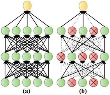

  

  An illustration of applying the dropout method to a standard neural network: a A standard neural network with 2 hidden layers before applying dropout method. b An example of a reduced neural network after applying dropout method. The crossed units and the dashed connections have been dropped

• 2. AdaGrad algorithm in the iris recognition system, infrequent features can significantly contribute to improving the accuracy of the system through minimizing intra-class variations and inter-class similarities, which is caused by several factors, including pupil dilation/constriction, eyelid/eyelash occlusion, and specular reflections spots. However, in the standard Stochastic Gradient Descent (SGD) algorithm for learning rate adaptation, both infrequent and frequent features are weighted equally in terms of learning rate, which means that the influence of the infrequent features is practically discounted. To counter this, the AdaGrad algorithm is implemented to increase the learning rate for more sparse data, which is translated into a larger update for infrequent features, and decreased learning rate for less sparse data, which is translated into a smaller update for the frequent features. The AdaGrad algorithm also has the advantage of being simpler to implement than the SGD algorithm [42]. The AdaGrad technique has been shown to improve the convergence performance stability of neural networks over the SGD in many different applications (e.g., NLP, document classification) in which the infrequent features are more useful than the more frequent features. The AdaGrad algorithm computes the learning rate η for every parameter $\left( {\varvec{\theta}_{\varvec{i}} } \right)$ at each time step $\varvec{t}$ based on the previous gradients of the same parameter as follows:

$$\varvec{\theta}_{\varvec{i}}^{{\left( {\varvec{t} + 1} \right)}} = \varvec{ \theta }_{\varvec{i}}^{{\left( \varvec{t} \right)}} - \varvec{ }\frac{\varvec{\eta}}{{\sqrt {\varvec{G}_{{\varvec{t},\varvec{ii}}} + \varvec{e}} }}\varvec{ }. \, \varvec{ g}_{{\varvec{t},\varvec{i}}} \varvec{ }$$

(8)

Here, $\varvec{g}_{{\varvec{t},\varvec{i}}} = \nabla_{\varvec{\theta}} \varvec{J}\left( {\varvec{\theta}_{\varvec{i}} } \right)$ is the gradient of the objective function at time step t, and $\varvec{G}_{{\varvec{t},\varvec{ii}}} = \mathop \sum \nolimits_{{\varvec{r} = 1}}^{\varvec{t}} \varvec{g}_{{\varvec{t},\varvec{i}}}^{2}$ is the diagonal matrix where each diagonal element (i, i) is the sum of the squares of the gradients for the parameter $\left( {\varvec{\theta}_{\varvec{i}} } \right)\varvec{ }$ at time step t. Finally, $\varvec{e}$ is a small constant to avoid division by zero. More details on the AdaGrad algorithm can be found in [42].

• 3. Data augmentation it is well known that DNNs need to be trained on a large number of training samples to achieve satisfactory prediction and prevent overfitting [45]. Data augmentation is a simple and commonly used method to artificially enlarge the dataset by methods such as random crops, intensity variations, horizontal flipping. In this work, data augmentation is implemented similarly to [14]. Initially, a given rectangular image is rescaled so that the longest side is reduced to the length of the shortest side instead of cropping out a square central patch from the rectangle image as in [14], which can lose crucial features from the iris image. Then, five image regions are cropped from the rescaled image corresponding to the four corners and central region. In addition, their horizontally flipped versions are also acquired. As a result, ten image patches are generated from each input image. During prediction time, the same ten image patches are extracted from each input image, and the mean of the predictions on the ten patches is taken at the Softmax layer. In this paper, the performance of the CNN is evaluated using two different input image sizes so the data augmentation procedure is implemented twice, once for each size. Image patches of size (64 × 64) pixels are extracted from original input images of size (256 × 70) pixels, and image patches of size (128 × 128) pixels are extracted from original input images of size (256 × 135) pixels.

• 4. The ReLU activation function is applied on the top of the convolutional and fully connected layers in order to add non-linearity to the network. As reported by Krizhevsky [14], the ReLU $\varvec{f}\left( \varvec{x} \right) = {\mathbf{max}}\left( {0,\varvec{x}} \right)\varvec{ }$ has been found to be crucial to learning when using DNNs, especially for CNNs, compared to other activation functions, such as the sigmoid and tangent. In addition, it results in neural network training several times faster than with other activation functions, without making a significant difference to generalization accuracy.

• 5. Weight decay is used in the learning process as an additional term in calculating the cost function and updating the weights. Here, the weight decay parameter is set to 0.0005 as in [46].

4.4 Ranking-level fusion

In this paper, rank level fusion is employed where each individual classifier produces a ranked list of possible matching scores for each user. (A higher rank indicates a better match). Then these ranks are integrated to create a new ranking list that is used to make the final decision on user identity. Suppose, that there are P persons registered in the database and the number of employed classifiers is C. Let r _{i, j} is the rank assigned to $\varvec{jth}$ person in the database by the $\varvec{ith}$ classifier, i = 1,…,C and j = 1,…,P. Then, the consensus ranks $\varvec{R}_{\varvec{c}}$ for a particular class are obtained using the following fusion methods:

• 1. Highest rank method is a useful method for fusing the ranks only when the number of registered users is large compared to the number of classifiers, which is usually the scenario in the identification system. The consensus rank of a particular class is computed as the lowest rank generated by different classifiers (minimum r _{i, j} value) as follows:

$$\varvec{R}_{\varvec{c}} = \varvec{ }\mathop {{\mathbf{min}}}\limits_{{1 \le \varvec{i} \le \varvec{ C}}} \varvec{r}_{{\varvec{i},\varvec{j}}} \varvec{ }$$

(9)

The main advantage of this method is the ability of exploiting the strength of each classifier effectively, where as long as there is at least one classifier that assigns a high rank r _{i, j} value to the right identity, it is very likely that the right identity will receive the highest rank value after the reordering process. However, the final ranking list may have one or more ties that can negatively affect the accuracy of the final decision. In this work, the ties are broken by incorporating a small factor epsilon (e), as described in [47] as follows:

$$\varvec{ R}_{\varvec{c}} = \varvec{ }\mathop {{\mathbf{min}}}\limits_{{1 \le \varvec{i} \le \varvec{ C}}} \varvec{r}_{{\varvec{i},\varvec{j}}} + \varvec{ e}_{\varvec{i}}$$

(10)

Here,

$$\varvec{e}_{\varvec{i}} = \varvec{ }\mathop \sum \limits_{{\varvec{i} = 1}}^{\varvec{C}} \varvec{r}_{{\varvec{i},\varvec{j}}} /\varvec{K }$$

(11)

Here, the value of $\varvec{e}_{\varvec{i}}$ is ensured to be small by assigning a large value to parameter K.

• 2. Borda count method using this fusion method, the consensus rank of a query identity is computed as the sum of ranks assigned by individual classifiers independently, as follows:

$$\varvec{R}_{\varvec{c}} = \varvec{ }\mathop \sum \limits_{{\varvec{i} = 1}}^{\varvec{C}} \varvec{r}_{{\varvec{i},\varvec{j}}} \varvec{ }$$

(12)

The main advantage of the Borda count method is that it is very simple to implement without the need for any training phase. However, this method is highly susceptible to the impact of weak classifiers, as it supposes that all the ranks produced by the individual classifiers are statistically independent and their performance is equally well [48].

• 3. Logistic regression method is a generalized form of the Borda count method to solve the problem of the uniform performance of the individual classifiers. The consensus rank is calculated by sorting the users according to the summation of their ranks obtained from individual classifiers, as follows:

$$\varvec{R}_{\varvec{c}} = \varvec{ }\mathop \sum \limits_{{\varvec{i} = 1}}^{\varvec{C}} \varvec{w}_{{\varvec{i*}}} \varvec{r}_{{\varvec{i},\varvec{j}}}$$

(13)

Here, $\varvec{w}_{\varvec{i}}$ is the weight to be assigned to the $\varvec{ith}$ classifier, i = 1,…,C, is determined by logistic regression. In this work, the $\varvec{w}_{\varvec{i}}$ is assigned to be 0.5 for both the left and right iris image. This method is very useful in the presence of different individual classifiers with significant differences in their performance. However, a training phase is needed to identify the weight for each individual classifier, which can be computationally expensive.

5 Experimental results

In this section, a number of extensive experiments to assess the effectiveness of the proposed deep learning approach for iris recognition on the most challenging iris databases currently available in the public domain are described. Three iris databases, namely, SDUMLA-HMT [49], CASIA-Iris-V3 Interval [50], and IITD [51] are employed as testing benchmarks and for comparing the results obtained with current state-of-the-art approaches. In most cases, the iris images in these databases were captured under different conditions of pupil dilation, eyelids/eyelashes occlusion, head-tilt, slight shadow of eyelids, specular reflection, etc. The SDUMLA-HMT iris database comprises 1060 images taken from 106 subjects with each subject providing 5 left and 5 right iris images. In this database, all images were captured using an intelligent iris capture device with the distance from the device to the eye between 6 cm and 32 cm. To the best of our knowledge, this is the first work that uses all the subjects in this database for the identification task. The CASIA-Iris-V3 Interval database comprises 2566 images from 249 subjects, which were captured with a self-developed close-up iris camera. In this database, the number of images of each subject differs and 129 subjects have less than 14 iris images. These were not used in the experiments. The IIT Delhi Iris database comprises 1120 iris images captured from 224 subjects (176 males and 48 females), who are students and staff at IIT Delhi, New Delhi, India. For each person 5 iris images for each eye were captured using three different cameras: JIRIS, JPC1000, and digital CMOS cameras. The basic characteristics of these three databases are summarized in Table 1.

Table 1 The characteristics of the adopted iris image databases

5.1 Iris localization accuracy

As explained in a previous paper [39], the performance of the proposed iris localization model was tested on two different databases, and showed encouraging results with overall accuracies of 99.07 and 96.99% on the CASIA Version 1.0 and the SDUMLA-HMT databases, respectively. The same evaluation procedure is applied herein in order to evaluate the performance of the iris localization model on the CASIA-Iris-V3 and IITD databases. The iris localization is considered accurate if and only if two conditions are fulfilled. Firstly, the inner and outer iris boundaries are correctly localized. Secondly, the upper and the lower eyelids boundaries are correctly detected. Finally, the accuracy rate of the proposed iris localization method is computed as follows:

$$\varvec{Accurcy \, Rate} = \varvec{ }\frac{{\varvec{Correctly \, Localized \, Iris \, Images}}}{{\varvec{Total \, Number}}}\varvec{ } \times 100\varvec{ }$$

(14)

As can be seen from Table 2, results with an overall accuracy of 99.82 and 99.87%, obtained with times of 0.65 s and 0.51 s, were achieved applying the proposed iris localization model on the CASIA-Iris-V3 and IITD database, respectively. The proposed model managed to properly detect the iris region from 1677 out of 1680 eye images in the CASIA-Iris-V3 Interval database, while 2237 iris images are properly detected out of 2240 eye images in the IITD database. The incorrect iris localization results have been taken into account manually to ensure that all the subjects have the same number of images for the subsequent evaluation of the overall proposed system.

Table 2 Comparison of the proposed iris localization model with previous approaches

Also, the performance of the proposed model is compared against other existing approaches. The results obtained demonstrate that the proposed system outperforms the indicated state-of-the-art of approaches in terms of accuracy in 14 out of 14 cases and in terms of running time in 6 out of 9 cases, where this information is available.

5.2 Finding the best CNN

In this section, extensive experiments performed to find the best CNN model (called IrisConvNet) for the iris recognition system, are described. Based on the domain knowledge in the literature, sets of training parameters and CNN configurations, as illustrated in Fig. 7, were evaluated to study their behavior and to obtain the best CNN. Then, the performance of this best system was used later on to make comparisons with current state-of-the-art iris recognition systems.

Fig. 7

An illustration of the IrisConvNet model for iris recognition

5.2.1 Training parameters evaluation

As mentioned previously, a set of training parameters is needed in order to study and analyze their influence on the performance of the proposed deep learning approach and to design a powerful network architecture. All these experiments were conducted on the three different iris databases, and the parameters with the best performance (e.g., lowest validation error rate and best generalization ability) were kept to be used later in finding the best network architecture. For an initial network architecture, the Spoofnet architecture as described in [15] was used with only a few changes. The receptive field in the first convolutional layer was set to be (3 × 3) pixels rather than (5 × 5) pixels to avoid a rapid decline in the amount of input data, and the output of the Softmax layer was set to N units (the number of classes) instead of 3 units as in the Spoofnet. Finally, the (64 × 64) input image size rather than (128 × 128) was used in these experiments with a zero padding of 1 pixel value applied only to the input layer. The first evaluation was to analyze the influence of the learning rate parameter using the AdaGrad optimization method. Based on the proposed training methodology, an initial learning rate of 10⁻³ was employed as in [62]. However, we observed that the model takes too long to converge because the learning rate was too small and it reduced continuously after each epoch according to the AdaGrad method. Therefore, for all the remaining experiments, an initial learning rate of 10⁻² was used. For the first time, the initial number of epochs was set to 100 epochs as in [14]. After that, larger numbers of epochs were also investigated using the same training methodology, including 200, 300, 400, 500 and 600 epochs. The CMC curves shown in Fig. 8 are used to visualize the performance of the last obtained model on the validation set. It can be seen that as long as the number of epochs is increased, the performance of the last model gets better. However, when 600 epochs were evaluated, it was observed that the obtained model started overfitting the training data and poor results were obtained on the validation set. Therefore, 500 epochs were taken as the initial number of epochs in our assessment procedure for all remaining experiments, since the learning process still achieved good generalization without overfitting.

Fig. 8

CMC curves for epoch number parameter evaluation using three different iris databases: a SDUMLA-HMT, b CASIA-Iris-V3, and c IITD

5.2.2 Network architecture and input image size evaluation

The literature on designing powerful CNN architectures shows that this is an open problem and usually approached using previous knowledge of related applications. Generally, the CNN architecture is related to the size of the input image. A smaller network architecture (a smaller number of layers) is required for a small image size to avoid degrading the quality of the last generated feature vectors by increasing the number of layers, while a deeper network architecture can be employed for input images with a larger size along with a large number of training samples to increase the generalization ability of the network by learning more distinctive features from the input samples. In this study, when the training parameters have been determined, the network architecture and input image size were evaluated simultaneously by performing extensive experiments using different network configurations. Based on the proposed training methodology, our evaluation strategy starts from a relatively small network (three layers), and then the performance of the network was observed by adding more layers and filters within each layer. In this work, the influence of input image size was investigated using image sizes of (64 × 64) pixels and (128 × 128) pixels, each with two different network configurations. For example, the (64 × 64) size was assessed using network topologies with 3 and 4 convolutional layers, while the (128 × 128) size was assessed using network topologies with 4 and 5 convolutional layers.

The results obtained by applying the proposed system on the three different iris databases with image sizes of (64 × 64) pixels and (128 × 128) pixels are presented in Tables 3 and 4, respectively. As can be seen in these tables, the number of the filters in each layer is tending to increase as one moves from the input layer toward the higher layers, as has been done in previous work in the literature, to avoid memory issues and control the model capacity. In general, it has been observed that the performance of a CNN improves as the number of the employed layers is increased along with the number of the filters per each layer. For instance, in Table 3 the recognition rate dramatically increased for all databases by adding a new layer on the top of the network. However, adding a new layer on the top of the network and/or altering the number of the filters within each layer should be carefully controlled. For instance, in Table 4, it can be seen that adding a new layer led to a decrease in the recognition rate from 93.02 to 80.09% for the left iris image in the SDUMLA-HMT database, and from 99.17 to 95.23% for the right iris image in the CASIA-Iris-V3 database. In addition, changing the number of filters within each layer has a significant influence on the performance of the CNN. Examples of this are shown in Table 3 (e.g., configuration number 10 and 11), and Table 4 (e.g., configuration number 18 and 19) where altering the number of filters in some layers has led to either an increase or a decrease in the recognition rate.

Table 3 Rank-1 identification rates obtained for different CNN architectures using the input image size of (64 × 64) pixels. Each configuration has either 3 or 4 layers and indicates the number of filters in each layer

Table 4 Rank-1 identification rates obtained for different CNN architectures using the input image size of (128 × 128) pixels. Each configuration has either 4 or 5 layers and indicates the number of filters in each layer

As indicated in Fig. 7, we prefer the last CNN configuration in Table 3 as the adopted CNN architecture for identifying a person’s identity for several reasons. Firstly, it provides the highest identification rate at Rank-1 for both the left and right iris images for all the employed databases with less complexity (fewer parameters). Secondly, although this model has given promising results using an input image of size (128 × 128) pixels, the input image size might be a major constraint in some applications; hence, the smaller one is used as the input image size for IrisConvNet. In addition, the training time required to train such a configuration is less than one day, as shown in Table 5. Finally, a larger CNN configuration along with a larger image size drives significant increases in memory requirements and computational complexity. The performance of IrisConvNet for iris identification for both employed input images sizes, is expressed through the CMC curve, as shown in Fig. 9. In this work, the running time was measured by implementing the proposed approaches using a laboratory in Bradford University consisting of 25 PCs with the Windows 8.1 operating system, Intel Xeon E5-1620 CPUs and 16 GB of RAM. The system code was written to run in MATLAB R2015a and later versions. Table 5 shows the overall average of the training time of the proposed system, which mainly depends on the input image size, the number of subjects in each database, and the CNN architecture.

Table 5 The average training time of the proposed system

Fig. 9

CMC curves for IrisConvNet for iris identification: a SDUMLA-HMT, b CASIA-Iris-V3, and c IITD

5.3 Fusion methods evaluation

Used as an iris identification system, each time a query sample is presented, the similarity score is computed by comparing it against the templates of N different subjects registered in the database and a vector of N matching scores is produced by the classifier. These matching scores are arranged in descending order to form the ranking list of matching identities where a smaller rank number indicates a better match. Table 6 shows the Rank-1 identification rate (%) for both left and right iris images in the SDUMLA-HMT, CASIA-Iris-V3, and IITD databases, and their fusion rates using the three ranking-level fusion methods: highest ranking, Borda count, and logistic regression. All three fusion methods produced the same level of accuracy, as shown in Table 6. The highest ranking method was adopted for comparing the performance of the proposed system with that of other existing systems, due to its efficiency compared to the Borda count method in exploiting the strength of each classifier effectively and breaking the ties between the subjects in the final ranking list. In addition, it is simpler than the logistic regression method, which needs a training phase to find the weight for each individual classifier. The comparison of the performance of the proposed system with the other existing methods using CASIA-Iris-V3 and ITD database is demonstrated in Table 7. The feature extraction and classification techniques used in these methods along with their evaluation protocols are shown in Table 8. We have assumed that these existing methods shown in Table 7 are customized for these two iris databases and the best results they obtained are quoted herein. As can be seen from inspection of Table 7, the proposed deep learning approach has overall, outperformed all the state-of-the-art feature extraction methods, which include Discrete Wavelet Transform (DWT), Discrete Cosine Transform (DCT), Principal Component Analysis (PCA), Average Local Binary Pattern (ALBP), etc. In term of the Rank-1 identification rate, the highest results were obtained by the proposed system using these two databases. Although Umer et al. [57] also achieved a 100% recognition rate for the CASIA-Iris-V3 database, the proposed system achieved a better running time to establish the person’s identity from 120 persons from the same database instead of 99 persons as in [57]. In addition, they obtained inferior results for the IITD database in terms of both recognition rate and running time.

Table 6 Rank-1 identification rate (%) of the proposed system on iris databases

Table 7 Comparison of the proposed system with other existing approaches using two different iris databases

Table 8 Summary of the compared iris recognition approaches and their evaluation protocols

6 Conclusions and future works

In this paper, a robust and fast multimodal biometric system is proposed to identify the person’s identity by constructing a deep learning based system for both the right and left irises of the same person. The proposed system starts by applying an automatic and real-time iris localization model to detect the iris region using CCHT, which has significantly increased the overall accuracy and reduced the processing time of the subsequent stages in the proposed system. In addition, reducing the effects of the appearance of the eyelids and eyelashes can significantly decrease the iris recognition performance. In this work, an efficient deep learning system based on a combination of the CNN and Softmax classifier is proposed and to extract discriminative features from the iris image without any domain knowledge and then classify it into one of N classes. After the identification scores and rankings are obtained from both the left and right iris images for each person a multi-biometric system is established by integrating these rankings to make a new ranking list using one of the ranking-level fusion techniques to formulate the final decision. Then, the performance of the identification system is expressed through CMC curve. In this work, we proposed a powerful training methodology equipped with a number of training strategies in order to control overfitting during the learning process and increase the generalization ability of the neural network. The effectiveness and robustness of the proposed approaches have been tested on three challenging databases: SDUMLA-HMT, CASIA-Iris-V3 Interval and IITD iris database. Extensive experiments have been conducted on these databases to evaluate different numbers of training parameters (e.g., learning rate, number of layers, number of filters per each layer) in order to build the best CNN as the framework for the proposed iris identification system. The experimental results demonstrated the superiority of the proposed system over recently reported iris recognition systems with a Rank-1 identification rate of 100% on all the three databases and less than one second required to establish the person’s identity. Clearly, further research will be required to validate the efficiency of the proposed approaches using larger databases with more difficult and challenging iris images. In addition, exploring the potential of using the proposed deep learning approaches on the top of pre-precessed iris images using some of well-known features extraction methods such as LBP and Curvelet transform. We might be able to guide the proposed deep learning approaches to explore more discriminating features otherwise not possible using the raw data.

References

Hajari K (2015) Improving iris recognition performance using local binary pattern and combined RBFNN. Int J Eng Adv Technol 4(4):108–112
Al-Waisy AS, Qahwaji R, Ipson S, Al-Fahdawi S (2015) A robust face recognition system based on curvelet and fractal dimension transforms. In: 2015 IEEE international conference computet information technology ubiquitous computing communication dependable, autonomic secure computing, pervasive intelligence computing. pp. 548–555
Tan T, Sun Z (2009) Ordinal measures for iris recognition. IEEE Trans Pattern Anal Mach Intell 31(12):2211–2226
Abiyev RH, Kilic KI (2011) Robust feature extraction and iris recognition for biometric personal identification. Biometric Syst Des Appl, InTech
Hentati R, Hentati M, Abid M (2012) Development a new algorithm for iris biometric recognition. Int J Comput Commun Eng 1(3):283–286
Das A, Parekh R (2012) Iris recognition using a scalar based template in eigen-space. Int J Comput Sci Telecommun 3(5):3–8
AlMahafzah H, Zaid AlRwashdeh M (2012) A survey of multibiometric systems. Int J Comput Appl 43(15):36–43
Gad R, EL-SAYED A, Zorkany M, El-fishawy N (2015) Multi-biometric systems: a state of the art survey and research directions. Int J Adv Comput Sci Appl 6(6):128–138
Ross A, Nandakumar K, Anil JK (2006) Handbook of multibiometrics. J Chem Inf Model 53(9):1689–1699
Fernandez FA (2008) Biometric sample quality and its application to multimodal authentication systems. PhD Thesis, Universidad Polit´ ecnica de Madrid (UPM)
Deng L, Yu D (2013) Deep learning methods and applications. Signal Process 28(3):198–387
Pellegrini T (2015) Comparing SVM, Softmax, and shallow neural networks for eating condition classification. In: Sixteenth annual conference of the international speech communication association. pp 899–903
Srivastava N, Hinton GE, Krizhevsky A, Sutskever I, Salakhutdinov R (2014) Dropout: a simple way to prevent neural networks from overfitting. J Mach Learn Res 15:1929–1958
Krizhevsky A, Sulskever I, Hinton GE (2012) ImageNet classification with deep convolutional neural networks. In: Advances in neural information processing system. pp 1–9
Menotti D, Chiachia G, Pinto A, Schwartz WR, Pedrini H, Falcão AX, Rocha A (2015) Deep representations for iris, face, and fingerprint spoofing detection. IEEE Trans Inf Forensics Secur 10(4):864–879
Silva P, Luz E, Baeta R, Pedrini H, Falcao AX, Menotti D (2015) An Approach to iris contact lens detection based on deep image representations. In: 2015 28th SIBGRAPI conference on graphics, patterns images. pp 157–164
Daugman JG (1993) High confidence visual recognition of persons by a test of statistical independence. IEEE Trans Pattern Anal Mach Intell 15(11):1148–1161
Ren X, Peng Z, Zeng Q, Peng C, Zhang J, Wu S, Zeng Y (2008) An improved method for Daugman’s iris localization algorithm. Comput Biol Med 38(1):111–115
Proenc H, Alexandre LA (2006) Iris segmentation methodology for non-cooperative recognition. IEE Proce Vis Image Signal Process 153(2):199–205
Sahmoud SA, Abuhaiba IS (2013) Efficient iris segmentation method in unconstrained environments. Pattern Recognit 46(12):3174–3185
Wildes RP (1997) Iris recognition: an emerging biometric technology. Proc IEEE 85(9):1348–1363
Boles WW, Boashash B (1998) A human identification technique using images of the iris and wavelet transform. IEEE Trans Signal Process 46(4):1185–1188
Lim S, Lee K, Byeon O, Kim T (2001) Efficient iris recognition through improvement of feature vector and classifier. ETRI J 23(2):61–70
Masek L (2003) Recognition of human iris patterns for biometric identification. The School of Computer Science and Software Eng- ineering, The University of Western Australia, Crawley
Ding S, Zhu H, Jia W, Su C (2011) A survey on feature extraction for pattern recognition. Artif Intell Rev 37(3):169–180
Jihua Y, Dan H, Guomiao X, Yahui C (2013) An advanced BPNN face recognition based on curvelet transform and 2DPCA. In: 8th international conference computer science education (ICCSE). pp 1019–1022
Khalajzadeh H, Mansouri M, Teshnehlab M (2014) Face recognition using convolutional neural network and simple logistic classifier. In: Soft computing in industrial application, Springer. pp 197–207
Zeng M, Nguyen LT, Yu B, Mengshoel OJ, Zhu J, Wu P, Zhang J (2014) Convolutional neural networks for human activity recognition using mobile sensors. In: 2014 6th international conference mobile computing, applications and services (MobiCASE). pp 197–205
Syafeeza AR, Liew SS, Bakhteri R (2014) Convolutional neural network for face recognition with pose and illumination variation. Int J Eng Technol 6(1):44–57
Collobert R, Weston J (2008) A unified architecture for natural language processing: deep neural networks with multitask learning. In: Proceedings on 25th international conference on machine learning. pp 160–167
Hafemann LG, Oliveira LS, Cavalin PR, Sabourin R (2015) Transfer learning between texture classification tasks using convolutional neural networks. In: International joint conference neural networks. pp 1–7
El Khiyari H, Wechsler H (2016) Face recognition across time lapse using convolutional neural networks. J Inf Secur 7(3):141–151
Dahl GE (2015) Deep learning approaches to problems in speech recognition, computational chemistry, and natural language text processing. PhD Thesis, Department of Computer Science, University of Toronto, p 101
Salakhutdinov R, Hinton G (2009) Semantic hashing. Int J Approx Reason 50(7):969–978
Ciresan DC, Meier U, Masci J, Schmidhuber J (2012) Multi-column deep neural network for traffic sign classification. Neural Netw 32:333–338
Abibullaev B, An J, Jin SH, Lee SH, Il Moon J (2013) Deep machine learning—a new frontier in artificial intelligence research. Med Eng Phys 35(12):1811–1818
Bengio Y (2009) Learning deep architectures for AI”, Found. Trends®. Mach Learn 2(1):1–127
Zeng R, Wu J, Shao Z, Senhadji L, Shu H, Zeng R, Wu J, Shao Z, Senhadji L, Shu H (2015) Quaternion softmax classifier. Electron Lett IET 50(25):1929–1930
Al-Waisy AS, Qahwaji R, Ipson S, Al-Fahdawi S (2015) A fast and accurate iris localization technique for healthcare security system. In: 2015 IEEE international conference computer and information technology; ubiquitous computing and communications; dependable, autonomic and secure computing; pervasive intelligence and computing. pp 1028–1034
Duda R, Hart P, Stork D (2012) Patterns classification. Wiley, New York
Sun Y, Wang X, Tang X (2014) Deep learning face representation from predicting 10,000 classes. In: Proceedings of the IEEE conference on computer vision and pattern recognition. pp 1891–1898
Duchi J, Hazan E, Singer Y (2011) Adaptive subgradient methods for online learning and stochastic optimization. J Mach Learn Res 12:2121–2159
Fergus R, Zeiler M (2015) Visualizing and understanding convolutional networks. In: European conference on computer vision. Springer, pp 818–833
Oquab M, Oquab M, Laptev I, Learning JS, Mid-level T, Oquab M, Bottou L (2014) Learning and transferring mid-level image representations using convolutional neural networks. In: IEEE conference on computer vision and pattern recognition
Al-Waisy AS, Qahwaji R, Ipson S, Al-Fahdawi S (2017) A multimodal deep learning framework using local feature representations for face recognition. Mach Vis Appl 1–20. doi:10.1007/s00138-017-0870-2
Turchenko V, Luczak A (2015) Creation of a deep convolutional auto-encoder in caffe. arXiv Prepr. arXiv1512.01596
Abaza A, Ross A (2009) Quality based rank-level fusion in multibiometric systems. In: Proceedings on 3rd IEEE international conference on biometrics: theory, applications, and systems. pp 1–6
Monwar MM, Gavrilova M (2013) Markov chain model for multimodal biometric rank fusion. Signal Image Video Process 7(1):137–149
Yin Y, Liu L, Sun X (2011) SDUMLA-HMT: a multimodal biometric database. In: Chinese conference on biometric recognition. Springer, Berlin Heidelberg, pp 260–268
Chinese Academy of Science—Institute of Automation, CASIA Iris Image Database Version 3.0 (CASIA-IrisV3). http://biometrics.idealtest.org/dbDetailForUser.do?id=3
Kumar A, Passi A (2010) Comparison and combination of iris matchers for reliable personal authentication. Pattern Recognit 43(3):1016–1026
Jan F, Usman I, Agha S (2012) Iris localization in frontal eye images for less constrained iris recognition systems. Digit Signal Process A Rev J 22(6):971–986
Wang K, Qian Y (2011) Fast and accurate iris segmentation based on linear basis function and RANSAC. In: Proceedings international conference on image processing ICIP, vol 2. pp 3205–3208
Mahlouji M, Noruzi A (2012) Human iris segmentation for iris recognition in unconstrained environments. Int J Comput Sci Issues 9(1):149–155
Uhl A, Wild P (2012) Weighted adaptive Hough and ellipsopolar transforms for real-time iris segmentation. In: Proceeding—2012 5th IAPR international conference on biometrics, ICB 2012. pp 283–290
Nkole IU, Bin Sulong G (2012) An enhanced iris segmentation algorithm using circle Hough transform. In: Proceedings of the IEEE international conference on Digital Signal and Image processing, pp 1–7
Umer S, Dhara BC, Chanda B (2016) Texture code matrix-based multi-instance iris recognition. Pattern Anal Appl 19(1):283–295
Version A (2015) Segmentation-level fusion for iris recognition. In: 14th international conference of the biometrics special interest group (BIOSIG 2015), pp 1–6
Aydi W (2011) Improved Masek approach for iris localization. In: ICM 2011 proceeding. IEEE, pp 1–5
Pawar MK, Student PG, Jhajjav G (2012) Iris segmentation using geodesic active contour for improved texture extraction in recognition. Int J 47(16):40–47
Mehrotra H, Sa PK, Majhi B (2013) Fast segmentation and adaptive SURF descriptor for iris recognition. Math Comput Model 58(1–2):132–146
Chowdhury AR, Lin T-Y, Maji S, Learned-Miller E (2016) One-to-many face recognition with bilinear CNNs. In: IEEE winter conference on applications of computer vision. pp 1–9
Ma L, Wang Y, Tan T (2002) Iris recognition using circular symmetric filters. In: 16th international conference on pattern recognition. pp 414–417
Vatsa M, Singh R, Noore A (2008) Improving iris recognition performance using segmentation, quality enhancement, match score fusion, and indexing. IEEE Trans Syst Man Cybern Part B Cybern 38(4):1021–1035
Kerim AA, Mohammed SJ (2014) New iris feature extraction and pattern matching based on statistical measurement. Int J Emerg Trends Technol Comput Sci 3(5):226–231
Da Costa RM, Gonzaga A (2012) Dynamic features for iris recognition. IEEE Trans Syst Man Cybern B Cybern 42(4):1072–1082
Ng TW, Tay TL, Khor SW (2010) Iris recognition using rapid Haar wavelet decomposition. In: 2010 2nd international conference on ignal processing systems (ICSPS), vol 1. pp V1-820–V1-823
Zhang H, Guan X (2012) Iris recognition based on grouping KNN and rectangle conversion. In: ICSESS 2012—Proceedings of 2012 IEEE 3rd international conference on software engineering and service science. pp 131–134
Roy K, Bhattacharya P, Suen CY (2011) Iris recognition using shape-guided approach and game theory. Pattern Anal Appl 14(4):329–348
Li C, Zhou W, Yuan S (2015) Iris recognition based on a novel variation of local binary pattern. Vis. Comput. 31(10):1419–1429
Bharath BV, Vilas AS, Manikantan K, Ramachandran S (2014) Iris recognition using radon transform thresholding based feature extraction with gradient-based isolation as a pre-processing technique. In: 9th international conference on industrial and information systems (ICIIS). IEEE, 2014, pp 1–8
Nalla PR, Chalavadi KM (2015) Iris classification based on sparse representations using on-line dictionary learning for large-scale de-duplication applications. Springerplus 4(1):1–10
Elgamal M, Al-Biqami N (2013) An efficient feature extraction method for iris recognition based on wavelet transformation. Int J Comput Inf Technol 2(3):521–527
Minaee S, Abdolrashidi A, Wang Y (2015) Iris recognition using scattering transform and textural features. In: Signal processing and signal processing education workshop (SP/SPE). IEEE, pp 37–42
Dhage SS, Hegde SS, Manikantan K, Ramachandran S (2015) DWT-based feature extraction and radon transform based contrast enhancement for improved iris recognition. Procedia Comput Sci 45(2015):256–265
Abhiram MH, Sadhu C, Manikantan K, Ramachandran S (2012) Novel DCT based feature extraction for enhanced iris recognition. In: Proceedings—2012 international conference on communication, information and computing technology ICCICT 2012. pp 1–6
Author information
Authors and Affiliations
Corresponding author
Rights and permissions
Open Access This article is distributed under the terms of the Creative Commons Attribution 4.0 International License (http://creativecommons.org/licenses/by/4.0/), which permits unrestricted use, distribution, and reproduction in any medium, provided you give appropriate credit to the original author(s) and the source, provide a link to the Creative Commons license, and indicate if changes were made.
About this article
Cite this article
Al-Waisy, A.S., Qahwaji, R., Ipson, S. et al. A multi-biometric iris recognition system based on a deep learning approach. Pattern Anal Applic 21, 783–802 (2018). https://doi.org/10.1007/s10044-017-0656-1
Received:
Accepted:
Published:
Issue Date:
DOI: https://doi.org/10.1007/s10044-017-0656-1