Genetic algorithm with aggressive mutation for feature selection in BCI feature space

Abstract

The aim of this paper is to present a new algorithm for feature selection, called a genetic algorithm with aggressive mutation. The paper presents both the theoretic background of the algorithm and its application for feature selection in the brain–computer interface (BCI) domain. To fully present the potential of the algorithm and to verify its practical usability, it is compared with other methods commonly used in BCI research. The practical application of the proposed algorithm is presented via a benchmark set submitted to the second BCI Competition (data set III—motor imagery).

1 Introduction

Assuming we record EEG signal from 32 electrodes and calculate the signal power in 5 frequency bands individually per each 5 s, the number of features in brain–computer interface (BCI) feature space amounts to 800 (32 electrodes $\times$ 5 frequency bands $\times$ 5 s). Hence, in the case of two classes, we need 1,600 observations to have only one observation per feature and per class. Since, it is recommended [1] to use at least 10 times more observations per class as the features, at least 16,000 observations would be necessary in the given example (800 features $\times$ 2 classes $\times$ 10 observations).

Carrying out 16,000 (or even 800) experiments in the case of analyzing EEG signals is impossible for at least several reasons. The first problem is the time that would be needed for dealing with this task. Assuming that one experiment takes 10 s, 16,000 experiments take 45 h. If it was possible to carry out the experiments simultaneously with 45 subjects, the task would not be so hard. Unfortunately, the oscillations forming EEG signals are subject specific, which means that all data applied to the classifier have to be collected from the same subject. The second problem is the habituation phenomenon [2], which can be described as a decrease in response to a stimulus after repeated presentations. And the last issue that should be mentioned here is that certain aspects of subject condition such as: high level of fatigue, varying level of concentration and attention, changes in mental condition, and changes in attitude towards the experiment are factors that may change the characteristic of the subject’s cortical rhythms [3].

As a result of the aforementioned facts, the number of records collected from one subject for the BCI training usually does not exceed 200–400. Such a small number of records allows building a classifier of about 9–18 features (assuming: 2 classes problem, 10 observations per each class and 90 % of data in the classifier training set). Comparing the huge dimension of the whole set of features that can be extracted from raw EEG signal with only several features that can be introduced to a classifier (according to Raundys recommendation [1]), it is obvious that a great reduction of the original feature space is needed.

The limited number of observations is not the only reason for using feature selection methods in BCI research. A smaller number of features is always wanted here, because it yields: higher speed, higher mobility, and lower costs of implementing the BCI, and above all—higher comfort for its user.

There are three main groups of feature selection methods [4, 5]: filters, wrappers and embedded methods. The characteristic feature of the methods from the first group is that they have no connection with the classification process. Hence, to use them, a classifier is not needed. Some popular methods from this group are [6, 7]: Information Gain, ReliefF, Correlation-based Feature Selection (CFS), and Consistency-based Feature Selection. On the contrary to the filters, wrappers and embedded methods need a classifier. While wrappers use a classifier only to evaluate succeeding feature subsets, embedded methods perform the selection as an inner process during the classifier training. The commonly used methods from both groups are: step-wise selection [8, 9], genetic algorithms [10] and random selection [11] (wrappers) and Recursive Feature Elimination [12], elastic net [13], and LASSO [14] (embedded methods).

One of the methods for feature selection, applied frequently in BCI domain, are genetic algorithms [2, 15]. Their main advantage is the fact that during the exploration of the space of possible solutions, they do not keep track of one trajectory of candidate solutions (like in gradient methods) but keep track of a set of candidates simultaneously. Moreover, they are not very prone to get stuck at local minima and they do not need assumptions about the interactions between features [16].

Another feature selection method from the wrappers group, popular in the domain of pattern recognition but rather rarely used in the BCI domain, is a step-wise selection. A step selection means that features are added to or removed from the feature set one by one in succeeding steps of the survey. The main drawback of this method is that it explores only one possible path in the search space, which made it prone to get stuck at local minima. This is true in general, however, when a very small subset of features is to be selected in the searching process, the step-selection method (to be exact, the forward step-selection method) is much more capable of finding such a small set of features of high discrimination capabilities [17] than a classic (Holland) genetic algorithm that is often applied in BCI research [2].

The aim of this paper is to present a new algorithm for feature selection, called the genetic algorithm with aggressive mutation (GAAM), proposed by the author during the CORES2013 conference [18]. The GAAM algorithm creates a link between both methods mentioned above—genetic algorithms and forward selection. On the one hand, it preserves the inherent advantages of the genetic algorithms—the capability of exploring distant areas of a feature space and avoiding getting stuck at local minima. On the other hand, it searches the feature space for a given, small number of features, as the forward selection method does.

The paper presents the theoretical aspects of the genetic algorithm with aggressive mutation and also the results of its application for selecting features extracted from a set of real EEG data. The data set that was used in the research was a set submitted to the second BCI Competition (data set III—motor imaginary) by Department of Medical Informatics, Institute for Biomedical Engineering, Graz University of Technology [19]. The practical usability of the GAAM algorithm was verified by comparing its results with results returned by other methods for feature selection, commonly used in BCI research. Although the genetic algorithm with aggressive mutation is a wrapper method, its results were compared with algorithms representing all three groups of feature selection methods: ReliefF (filter method), forward selection (wrapper method), and LASSO (embedded method). The algorithms results were compared in terms of classification accuracy.

The GAAM algorithm is dedicated not only for EEG analysis but can be used also for other multidimensional tasks, like for example ECG [20]).

2 Genetic algorithm with aggressive mutation (GAAM)

Genetic algorithm (GA) is a heuristic method for solving optimization problems. Nowadays, this method is used in many different research fields, but it originates from genetic sciences. To run the optimization process with a GA, first, the following aspects of the algorithm has to be defined:

• a method for coding problem solutions to the form of GA individuals (composed of chromosomes and genes),

• a fitness function used for evaluating individuals in each generation,

• genetic operations used for mixing and modifying individuals,

• a method for selecting individuals and other additional GA parameters.

When a GA is used in the feature selection process, each individual encodes one subset of features. The algorithm processes these individuals (i.e., different subsets of features) to obtain new individuals (i.e., new subsets of features) of higher discrimination capabilities. To compare the discrimination capabilities of individuals from the current population, a classifier is implemented for each individual.

The most popular approach adopted when a GA is to be used in the feature selection process is a classic genetic algorithm originally proposed by Holland. With this approach, the number of genes of an individual is the same as the number of features in the original feature space and each gene informs whether the corresponding feature is present in the solution that is encoded within an individual or not [2, 10].

The classic genetic algorithm has one essential drawback, when it is used as a feature selection method. The problem is that if we apply the uniform probability distribution while selecting the initial population, each individual will contain about half of all the possible features. Since evolution, guided by classification accuracy, favors individuals providing more training parameters for the classifier, i.e., individuals containing more features, we cannot expect that these initial individuals evolve to contain smaller number of features. In fact, the actual size of the final feature set returned by the algorithm will be very similar to the initial one.

Theoretically, the selection process does not have to be guided only by the classification accuracy. It is possible, for instance, to equip the GA fitness function with a penalty term, which will punish the individuals coding too many features. It is also possible to develop some specialized genetic operators converting such unwelcome individuals into individuals including a smaller number of features. In BCI research, however, the scale of the required reduction of the feature set is so large (usually higher than 95 % of all the features from the original feature set) that it is extremely difficult to develop such a function penalizing individuals carrying too many features or such functions for converting these individuals that will be appropriate for all possible problems’ settings. A much more convenient solution seems to be to define such a way of encoding individuals and such genetic operators that will permit the algorithm to process only feature subsets of a given size.

A genetic algorithm with aggressive mutation fulfills the above condition, because its problem space is composed only of individuals containing a fixed (and very small) number of genes. Each gene carries out the information about one of the features from the feature set encoded in an individual. Since GAAM uses integer coding system, each gene takes an integer value from the set $\{0,1,\ldots ,P\}$, where $P$ denotes the dimension of the whole feature set. The values from 1 to $P$ correspond to feature indexes and the value zero means no feature. Every time when the value zero occurs in an individual, the number of inputs of a classifier implemented for this individual is reduced by one. The number of genes of an individual is a GAAM parameter and is set at the beginning of the algorithm in relation to the number of observations, classifier mapping function and the overall characteristic of a problem at hand. The fitness function that is used to evaluate individuals is based directly on the classification accuracy. The GAAM algorithm is composed of the following steps.

• 1. Determine algorithm parameters: $T$—number of generations, $M$—number of individuals in a population, and $N$—number of genes in an individual.

• 2. Create an initial population of $M$ individuals. The population is created randomly by choosing values for succeeding genes from the set $\{0,1,\ldots ,P\}$.

• 3. Perform aggressive mutation on individuals from the previous population. As a result of the mutation operation, one parent individual has a set of $N$ off-springs, each created by mutating another gene of that individual. The mutation scheme, given in a pseudo-code, is as follows:

  

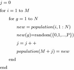
  where $population$—matrix of individuals, $new$—vector containing all genes of $i$th individual, random({$0,1,\ldots ,P$})—function that randomly draws a feature from the feature set.

• 4. Perform the classic Holland crossover on the individuals from the previous population (with a probability equal to one).

• 5. Create a mother population, containing $M$ individuals from the previous population, $NM$ individuals created during the aggressive mutation operation and $M$ individuals created during the crossover operation.

• 6. Evaluate the quality of the individuals from the mother population using classification accuracy as a fitness function.

• 7. Discard $M+MN$ individuals of the lowest classification accuracy. After this step, only $M$ individuals providing the highest classification accuracy remain in the population. Since all the best individuals from the previous population take part in the selection process, the best individual in the current population has at least the same fitness value as in the previous one.

• 8. Return to the step 3.

The algorithm permits individuals to include the same feature more than once. Each time when an individual with duplicated features appears (as a result of genetic operations or as a result of random initialization of the initial population), all identical genes (apart from one) are set to zero. As a result, a classifier obtains less inputs and it is possible to test whether the same classification precision cannot be obtained with a smaller number of features.

The algorithm is performed $T$ times in a loop. Three main parts of this loop determine the algorithm complexity: crossover, mutation and evaluation. The complexity of crossover for a single generation is $O(M)$ and the complexity of mutation and evaluation is $O(NM)$. Hence, the overall complexity of the whole algorithm is $O(TNM)$.

3 Applied methods

To verify the practical usability of the algorithm with aggressive mutation, three popular methods for feature selection were used: ReliefF, forward selection and LASSO.

3.1 The ReliefF algorithm

The ReliefF [21] algorithm is an extension of the Relief algorithm, proposed in 1992 by Kira and Rendell in [22, 23]. The difference between both algorithms is that the original Relief algorithm was limited to classification problems with only two classes and the extended version can deal with multiclass problems. The ReliefF algorithm estimates the relevance of features according to how well their values distinguish between instances that are near to each other. The general scheme of the algorithm is as follows. At first, a random instance $R_i$ from the training set is selected. Then, the algorithm searches for $k$ of its nearest neighbors from the same class (nearest hits $H_j$, where $j=\{1,\ldots ,k\}$) and for $k$ nearest neighbors from each of the remaining classes (nearest misses $M_j(C)$). Next, the feature relevance index is updated. In the updating formula, values of features for $R_i$, $H_j$ and $M_j(C)$ are analyzed:

• for each pair of $R_i$ and $H_j$: if the instances $R_i$ and $H_j$ have different values of the feature $A$, then the relevance of this feature is decreased,

• for each pair of $R_i$ and $M_j(C)$: if instances $R_i$ and $M_j(C)$ have different values of the feature $A$, then the relevance of this feature is increased.

To obtain the final quality estimation for a feature $A$, the contributions from all pairs of $R_i$-$H_j$ (pairs of hits) are averaged. The same is done with all pairs of $R_i$-$M_j(C)$ (pairs of misses), but in this case the contribution for each class of the misses is also weighted with the prior probability of that class $P(C)$ (estimated from the training set). The whole algorithm is repeated $m$ times. Parameter $m$ represents the number of instances from the training set that are used for approximating probabilities. In the case of small training sets, $m$ is equal to the number of training instances. When the training set is too big to examine all instances, $m$ value is chosen by the user.

Since the algorithm is based on the concept of the nearest neighborhood, their results strongly depend on the size of the neighborhood $k$. If $k$ is set to 1, the results of the algorithm can be unreliable for noisy data. If, on the other hand, $k$ is set to the number of observations, the algorithm can fail to find relevant attributes. Therefore, when ReliefF algorithm is used, different values of $k$ should be examined.

3.2 Forward selection

The step-selection methods are heuristic approaches that define the overall strategy of the searching process. Usually, three main methods are listed in this group [8]: forward selection, backward selection, and bidirectional selection. The only difference between all of them is the direction of the search. In the case of the first method, the selection process starts with an empty set of features. The set is then extended by adding one feature at each step of the procedure. Each time this feature is added to the set that provides the highest increase in the classification accuracy. The whole process ends when none of the remaining features is able to improve the classifier’s performance.

In the case of backward selection, the selection process starts with a set containing all the possible features, which are then one by one removed from the set. Of course, this time this feature is removed from the set that causes the smallest (or none) decrease in the classification accuracy. The last method is a simple mix of forward and backward selection—both elementary strategies are used alternately.

The decision whether to use a forward or backward selection is always determined by the characteristics of a given data set. In the case of BCI research, the forward selection is the only choice because of a huge feature space and a very limited number of observations.

3.3 LASSO

The Least Absolute Shrinkage and Selection Operator (LASSO) algorithm was proposed by Tibshirani [14]. The algorithm is a shrinkage and selection method for linear regression. The goal of the algorithm is to minimize the residual sum of squared errors with a bound on the sum of the absolute values of the linear regression coefficients that has to be less than a given constant. Because of the nature of this constraint, LASSO tends to produce some coefficients that are exactly $0$ and hence automatically discards features corresponding to these coefficients. LASSO minimizes:

$$\begin{aligned} \left( \frac{1}{2N}\sum _{i=1}^{N}(y_{i}-\beta _{0}-x_{i}^{T}\beta )^{2}+\lambda \sum _{j=1}^{p}|\beta _{j}|\right) , \end{aligned}$$

(1)

with respect to $\beta _{0}$ and $\beta$, where $N$ is the number of observations, $y_i$ is the response for observation $i$, $x_i$ is the $p$-dimensional input vector for observation $i$, $\lambda$ is a nonnegative regularization parameter, $\beta _0$ and $\beta$ are regression parameters ($\beta _0$ is a scalar, $\beta$ is a $p$-dimensional vector).

The number of nonzero components of $\beta$ found by the algorithm depends on the regularization parameter $\lambda$. As $\lambda$ increases, the number of nonzero components of $\beta$ decreases.

4 Experiment settings

To verify the practical usability of the genetic algorithm with aggressive mutation, a data set submitted to the second BCI Competition (data set III—motor imaginary) by Department of Medical Informatics, Institute for Biomedical Engineering, Graz University of Technology [19] was used. The data set was recorded from a normal subject (female, 25 years) whose task was to control the movements of a bar displayed on a screen by means of imagery movements of the left and right hand. Cues informing about the direction in which the bar should be moved were displayed on a screen as left and right arrows. The order of left and right cues was random. The experiment consisted of 280 trials, each lasting 9 s. The first 2 s were quiet. At $t$ = 2 s, an acoustic stimulus was generated and a cross ‘+’ was displayed for 1 s. Then, at $t$ = 3 s, an arrow (left or right) was displayed as a cue. The EEG signals were measured over three bipolar EEG channels (C3, Cz and C4), sampled with 128 Hz and preliminary filtered between 0.5 and 30 Hz. The whole data set, containing data from 280 trials, was then divided into two subsets of equal size—the first one intended for a classifier training and the second intended for an external classifier testing. Since only data from the first subset had been published with target labels (‘1’—left hand, ‘2’—right hand), only this subset alone was used in the experiments described in this paper.

The original data set, after removing the mean values from each channel, was transformed to a set of 324 frequency band power features. The band power was calculated separately for:

• 12 frequency bands: alpha band (8–13 Hz) and five sub-bands of alpha band (8–9 Hz; 9–10 Hz; 10–11 Hz; 11–12 Hz; 12–13 Hz); beta band (13–30 Hz) and also five sub-bands of beta band (13–17 Hz; 17–20 Hz; 20–23 Hz; 23–26 Hz; 26–30 Hz),

• each of 9 s of the trial,

• each of three channels (C3, Cz, C4).

During the experiments, features were identified according to their indexes. The full matrix of features’ indexes is given in Table 1.

Table 1 The matrix of features’ indexes

In the next stage of the experiment, the feature selection process was performed. The genetic algorithm with aggressive mutation, together with three other algorithms, described in Sect. 3, was used in this process. Feature subsets returned by each of the four algorithms were compared in terms of classification accuracy.

A classic linear SVM algorithm was used in the classification process [16, 24]. Before running the algorithm, class labels were changed to $-1$ for the left hand and 1 for the right hand. The classification threshold was set to 0 and hence all the classifier results greater than 0 were classified as ‘right hand’ and all results smaller or equal to 0 were classified as ‘left hand’. The classifier accuracy was tested with tenfold cross-validation. The mean value calculated over the classification accuracy obtained for all ten validation sets was the final accuracy measure used for comparing different feature sets.

To ensure comparable conditions for all four methods, the upper limit for the size of the feature set returned by each method was set. To establish this limit, Raudys recommendation about 10 observations per feature and per class was taken into account [1]. According to this recommendation, the final feature set had to contain six or less features (126 observations in each training set vs. 120 observations needed for the classifier of six inputs).

5 Results

The first method that was used for selecting relevant features from the whole set of features was the genetic algorithm with aggressive mutation. The algorithm parameters were set as follows—number of individuals ($M$): 10, number of genes in an individual ($N$): 6, number of iterations ($T$): 100. The initial population was chosen randomly (using uniform probability distribution). Two genetic operations were applied: one-point crossover (with a probability of 1) and aggressive mutation (according to the scheme presented in Sect. 2). After 100 iterations, the algorithm was terminated and the individual that achieved the highest value of the fitness function was accepted as the best one. The whole algorithm was run ten times. The classification accuracy of the best individual from each run is presented in Table 2 and the average fitness obtained for succeeding populations in each run is presented in Fig. 1.

Table 2 Results returned by the genetic algorithm with aggressive mutation in each run)

Fig. 1

The average fitness of populations returned in succeeding GAAM iteration. Each curve corresponds to different run of the algorithm

The second algorithm used for feature selection was ReliefF. Since results returned by this algorithm strongly depend on the size of the neighborhood $k$, the algorithm was run seven times for different $k$ values. The classification accuracy calculated for the set of the first six features returned by the algorithm in each run is presented in Table 3.

Table 3 Results returned by ReliefF algorithm for different size of the nearest neighborhood $k$

To apply the next method for feature selection—forward selection— the experiment had to be divided into six stages. In the first stage, 324 one-input classifiers, each containing another feature from the feature set, were implemented. After evaluating the accuracy of the classifiers, the feature used in the classifier of the highest accuracy was picked out. In the second stage, 323 two-input classifiers were built. Each classifier contained the feature chosen in the previous stage and one of the remaining features. Once again the accuracy of the classifiers was evaluated and the classifier of the highest accuracy was chosen and its input features were passed to the next stage. The same scheme was repeated in succeeding four stages. Table 4 presents the indexes of features that were added to the feature set at each stage of the experiment, together with the classification accuracy of the classifier chosen at each stage.

Table 4 Results returned by the forward selection algorithm in succeeding stages of the experiment

The last feature selection method that was used in the survey was LASSO. Since LASSO is an analytic procedure, the algorithm was run only once. The Matlab function lasso was used for the calculations. This function is able to calculate the best lambda parameter on itself taking into account the maximum number of nonzero coefficients in the model (DFmax) given by the user.

At first, DFmax was set to 6, however, only five features (104, 86, 5, 24, and 87) were returned with this setting. Hence, DFmax was enlarged to 7. This time a 7-feature set, composed of features: 104, 86, 5, 24, 87, 199 and 156, was returned. The accuracy of the classifier built with the 5-feature set was equal to 90.00 %, and the accuracy of the classifier built with the 7-feature set was only a little higher—it was equal to 90.71 %. Hence, even the 7-feature set returned with LASSO had lower classification accuracy than the worst feature set, returned by GAAM algorithm (92.14 %).

6 Discussion

Two facts can be noticed after a closer look at Table 2, presenting the results returned by the genetic algorithm with aggressive mutation. First, the classification accuracy obtained from 10 algorithm runs was very high. Such a high accuracy, obtained with a classifier equipped with only 5–6 input features, meant that the algorithm indeed chose the features significant for the classification process. Another very important fact is that similar feature subsets were returned in different GAAM runs. Only 15 out of 59 genes from the final population encoded features that did not repeat in different runs. The remaining 44 genes encoded 11 features that appeared in different combinations. Some of them appeared even in more than 50 % of the total number of runs (e.g., feature no. 104 in eight runs, feature no. 24 in seven runs, and feature no. 5 in six runs). This means that the algorithm behavior was stable and additionally underlines the fact that the selected feature subsets were of a high quality. Taking into account all ten best individuals, it can be noticed that from the whole set of 324 features, only 25 features were selected as important.

One might ask why the algorithm did not return exactly the same subset of features. The most straightforward explanation to this question is connected with the correlation between features. Since some of the extracted features were highly correlated, any swaps between them did not yield any difference in the classification accuracy. The five pairs of features of the highest Pearson coefficients were: features #5 and #86 (with a correlation of 96 %), features #6 and #87 (with a correlation of 95 %), features #23 and #104 (with a correlation of 95 %), features #24 and #105 (with a correlation of 95 %) and features #26 and #107 (with a correlation of 94 %).

Although the algorithm returned ten feature sets of a very similar classification accuracy, the final choice of the feature set that should be used in practice is rather simple. The best feature set is the set no. 8. This set gives the highest rate of the classification precision (94.29 %) and is composed of the smallest number of features (5 features).

One more issue is worth mentioning here—a very quick convergence of the algorithm. Although the algorithm was run for 100 generations, only 20 were enough to obtain the final result. As it can be noticed in Fig. 1, the average fitness of the population changes very quickly from 0.65–0.7 to 0.88–0.93 during the first 20 generations and then during the next 80 generations rises only very slightly to the final level of 0.89–0.94.

The classifier that was built over the feature set returned by the genetic algorithm with aggressive mutation, described in this paper, had a very high classification accuracy. None of the classifiers that were built over any of the feature sets returned by the remaining methods applied in the survey had higher or even the same classification accuracy. What is even more, none of the feature sets returned by any of those methods was at least equally good, in terms of classification accuracy, as the worst feature set obtained with GAAM.

7 Conclusion

The classification accuracy, exceeding 92 % in all 10 algorithm runs, is really a good result. Moreover, this result was obtained with linear SVM classifiers equipped with only 5 or 6 features, which allows to believe in high generalization capabilities of the final models.

Coming to future work, it should be stated that feature subsets returned by the proposed algorithm were similar but not the same. It could mean that the features were highly correlated, as it was stated in the paper, but it could also mean that six features were still too many for the given problem and that the similar accuracy could be obtained with even a smaller number of features. Hence, the issue that should be addressed now is how to force the algorithm to evaluate feature subsets containing less than $N$ features. It seems that to deal with this task, a specialized genetic operators aimed directly at reducing the number of features should be developed and introduced to the algorithm.

References

Raudys S, Jain A (1991) Small sample size effects in statistical pattern recognition: recommendations for practitioners. IEEE Trans Pattern Anal Mach Intell 13(3):252–264
Peterson D, Knight J, Kirby M, Anderson Ch, Thaut M (2005) Feature selection and blind source separation in an EEG-based brain–computer interface. EURASIP J Appl Signal Process 19:3128–3140
Sałabun W (2014) Processing and spectral analysis of the raw EEG signal from the MindWave. Przeglad Elektrotechniczny, SIGMA-NOT Sp. z o.o. 90(2):169–174
Saeys Y, Inza I, Larraaga P (2007) A review of feature selection techniques in bioinformatics. Bioinformatics 23(19):2507–2517
Liu H, Motoda H (1998) Feature selection for knowledge discovery and data mining. Kluwer Academic Publishers, Norwell
Koprinska I (2010) Feature selection for brain–computer interfaces. In: New frontiers in applied data mining, pp 106–117
Hall MA (1999) Correlation-based feature selection for machine learning. PhD thesis, The University of Waikato
Kittler J (1978) Feature set search algorithms. In: Pattern recognition and signal processing. Sijthoff and Noordhoff, Alphen aan den Rijn, The Netherlands, pp 41–60
Rejer I (2012) EEG feature selection for BCI based on motor imaginary task. Found Comput Decision Sci 37(4):283–292
Garrett D, Peterson D, Anderson Ch, Thaut M (2003) Comparison of linear, nonlinear, and feature selection methods for EEG signal classification. IEEE Trans Neural Syst Rehabil Eng 11(2):141–145
Burduk R (2012) Recognition task with feature selection and weighted majority voting based on interval-valued fuzzy sets. In: Nguyen N-T, Hoang K, Jdrzejowicz P (eds)Computational collective intelligence. Technologies and applications. Springer, Berlin, pp 204–209
Guyon I, Weston J, Barnhill S, Vapnik V (2002) Gene selection for cancer classification using support vector machines Machine learning. Springer 46(1–3):389–422
Zou H, Hastie T (2005) Regularization and variable selection via the elastic net. J R Stat Soc Ser B 67(2):301–320
Tibshirani R (1996) Regression shrinkage and selection via the lasso. J R Stat Soc Ser B 58(1):267–288
Yom-Tov E, Inbar G (2002) Feature selection for the classification of movements from single movement-related potentials. IEEE Trans Neural Syst Rehabil Eng 10(3):170–177
Lakany H, Conway B (2007) Understanding intention of movement from electroencephalograms. Expert Syst 24(5):295–304
Rejer I, Lorenz K (2013) Genetic algorithm and forward selection for feature selection in EEG feature space. J Theor Appl Comput Sci 7(2):72–82
Rejer I (2013) Genetic algorithms in EEG feature selection for the classification of movements of the left and right hand. In: Proceedings of the 8th international conference on computer recognition systems CORES 2013. Springer, Berlin, pp 579–589
http://bbci.de/competition/ii/index.html; data set III, II BCI Competition, motor imaginary
Augustyniak P (2010) Autoadaptivity and optimization in distributed ECG interpretation. In: Transactions on information technology in biomedicine, vol 14, no. 2. IEEE, New York, pp 394–400
Kononenko I (1994) Estimating attributes: analysis and extensions of Relief. In: De Raedt L, Bergadano F (eds) Machine learning: ECML-94. Springer, Berlin, pp 171–182
Kira K, Rendell L (1992a) The feature selection problem: traditional methods and new algorithm. In: Proceedings of AAAI92
Kira K, Rendell L (1992b) A practical approach to feature selection. In: Sleeman D, Edwards P (eds) Machine learning: proceedings of international conference (ICML92). Morgan Kaufmann, Burlington, pp 249–256
Schlögl A, Lee F, Bischof H, Pfurtscheller G (2005) Characterization of four-class motor imagery EEG data for the BCI-competition 2005. J Neural Eng IOP Publ 2(4):L14–L22
Author information
Authors and Affiliations
Corresponding author
Rights and permissions
Open Access This article is distributed under the terms of the Creative Commons Attribution License which permits any use, distribution, and reproduction in any medium, provided the original author(s) and the source are credited.
About this article
Cite this article
Rejer, I. Genetic algorithm with aggressive mutation for feature selection in BCI feature space. Pattern Anal Applic 18, 485–492 (2015). https://doi.org/10.1007/s10044-014-0425-3
Received:
Accepted:
Published:
Issue Date:
DOI: https://doi.org/10.1007/s10044-014-0425-3