New Examples on Lavrentiev Gap Using Fractals

Abstract

Zhikov showed 1986 with his famous checkerboard example that functionals with variable exponents can have a Lavrentiev gap. For this example it was crucial that the exponent had a saddle point whose value was exactly the dimension. In 1997 he extended this example to the setting of the double phase potential. Again it was important that the exponents crosses the dimensional threshold. Therefore, it was conjectured that the dimensional threshold plays an important role for the Lavrentiev gap. We show that this is not the case. Using fractals we present new examples for the Lavrentiev gap and non-density of smooth functions. We apply our method to the setting of variable exponents, the double phase potential and weighted p-energy.

1 Introduction

The Lavrentiev gap is a phenomenon that may occur in the study of variational problems. In particular, the minimum of the integral functional ${\mathcal {G}}$ taken over smooth functions may differ from the one taken over the associated energy space.

The first example for Lavrentiev gap was constructed by Lavrentiev in [14]. A simpler one was provided by Manià in [15], who considered the functional

subject to the boundary condition $w(0)=0$ and $w(1)=1$. Now, Manià showed that there exists $\tau > 0$ such that ${\mathcal {G}}(w) \ge \tau$ for all $w \in C^1([0,1])$ with $w(0)=0$ and $w(1)=1$. However, the function $x^{\frac{1}{3}} \in W^{1,1}((0,1))$ has strictly smaller energy, namely ${\mathcal {G}}(x^{\frac{1}{3}})=0$. This gap between zero and $\tau$ is the so called Lavrentiev gap.

In the example of Manià the integrand depends on x, w and $\xi$. If the integrand only depends on x and $\xi$, then the Lavrentiev gap does not appear in the case of one-dimensional problems, see [14]. The corresponding question for two and higher dimensional problems with integrands of the form $f(x,\nabla w(x))$ remained open for a very long time.

1.1 Zhikov’s Famous Checkerboard Example – Variable Exponents

In 1986 Zhikov presented his famous two-dimensional checkerboard example with a Lavrentiev gap, see [19]. In particular, he considered the functional

with the variable exponent (see Figure 1)

$$\begin{aligned} p(x)&:= {\left\{ \begin{array}{ll} p_2 &{}\qquad \hbox { for}\ x_1 x_2 > 0, \\ p_1 &{}\qquad \hbox { for}\ x_1 x_2 < 0, \end{array}\right. } \end{aligned}$$

where $1< p_1< 2 < p_2$ and $b \in L^{p'(\cdot )}(\Omega )$ with $\frac{1}{p'(x)} +\frac{1}{p(x)}=1$. At this $L^{p(\cdot )}(\Omega )$ denotes the space of Lebesgue space with variable exponent p. The natural energy space for this functional is $W^{1,{p(\cdot )}}_0(\Omega )$, the space of functions $w \in W^{1,1}_0(\Omega )$ with $\nabla w \in L^{p(\cdot )}(\Omega )$. See Subsections 3.1 and 4.1 for a precise definition of all function spaces. Now, Zhikov constructed a special vector field $b \in L^{{p'(\cdot )}}(\Omega )$ such that the infimum of ${\mathcal {G}}$ taken over $W^{1,{p(\cdot )}}_0(\Omega )$ is strictly smaller than the one taken over the smooth functions $C^\infty _0(\Omega )$. If we denote by $H^{1,{p(\cdot )}}_0(\Omega )$ the closure of $C^\infty _0(\Omega )$ in $W^{1,{p(\cdot )}}(\Omega )$, then we can summarize his result as

$$\begin{aligned} \inf {\mathcal {G}}\big (W^{1,{p(\cdot )}}_0(\Omega ) \big )&< \inf {\mathcal {G}}\big (H^{1,{p(\cdot )}}_0(\Omega )\big ) =0. \end{aligned}$$

The important feature of this example is that the exponent p has a saddle point, where it crosses the dimensional threshold, i.e. $p_1< 2 < p_2$. Moreover, the vector field b satisfies  in the sense of distributions, so $\int _\Omega b \cdot \nabla w\,dx=0$ for $w \in C^\infty _0(\Omega )$. However, for a suitable cut-off function $\eta \in C^\infty _0(\Omega )$, we have $\int _\Omega b \cdot \nabla (\eta u) \,dx = -1$ (see Proposition 24 and 25 ). Thus, b doesn’t see the gradients of $C^\infty _0(\Omega )$-functions but it sees the one of $\eta u \in W^{1,{\phi (\cdot )}}_0(\Omega )$. Therefore, the vector field b is also called separating vector field. Another useful feature is that almost everywhere.

The question of the Lavrentiev gap is closely related to the density of smooth functions, i.e. if $W^{1,{p(\cdot )}}_0(\Omega ) = H^{1,{p(\cdot )}}_0(\Omega )$ and $W^{1,{p(\cdot )}}(\Omega ) = H^{1,{p(\cdot )}}(\Omega )$. Using his checkerboard exponent Zhikov showed that the function (see Figure 1)

defined in polar coordinates $x=(r\cos \theta ,r \sin \theta )$ satisfies $u \in W^{1,{p(\cdot )}}(\Omega ) \setminus H^{1,{p(\cdot )}}(\Omega )$.

The vector field $b \in L^{p'(\cdot )}(\Omega )$ is in Zhikov’s example defined as $b(x) := \nabla ^\perp (u(x^\perp ))$ with $x^\perp = (-x_2,x_1)$ and $\nabla ^\perp = (-\partial _2,\partial _1)$, see [22, Section 3].

Fig. 1

Zhikov’s checkerboard example; $1< p_1< 2 < p_2$. The lines indicate smooth transitions

Now, $u \notin W^{1,p_2}(\Omega )$, since $p_2>2=d$ and u jumps at the point 0. But, since u changes its value in the area of the exponent $p_1 <2$, we still get $u \in W^{1,p(\cdot )}(\Omega )$.

However, u cannot be approximated by smooth functions $u_n$. Indeed, it follows from $u_n\in W^{1,p_2}(Q_1) \cap W^{1,p_2}(Q_3)$ and the continuity of $u_n$ at 0 that the $u_n$ are Hölder continuous on $\overline{Q_1} \cup \overline{Q_3}$ with exponent $\alpha := 1-\frac{2}{p_2}>0$ uniformly in n, but the limit u is not even continuous.

It is possible to generalize this example to higher dimensions, i.e. $\Omega = (-1,1)^d$ with $d\ge 2$. Again the variable exponent p has a saddle point at zero. It takes the value $p_2 > d$ on the double cone , and $p_1 < d$ on its complement. The crucial point is again that  for $\alpha = 1-\frac{d}{p_2}$. So the exponent has a saddle point, where it just crosses the dimension d.

Up to now no other examples of $H^{1,{p(\cdot )}}(\Omega ) \ne W^{1,{p(\cdot )}}(\Omega )$ with variable exponents were known. This led people to the question if the dimension plays a critical role, i.e. that it is important that at the saddle point the variable exponent p crosses the threshold d. This question has been repeatedly raised by Zhikov and also by Hästö [6].

The saddle point setup is the simplest geometry for the Lavrentiev gap to appear. It has been shown by Zhikov [19] that if ${p(\cdot )}$ takes only two values separated by a smooth surface, then $H^{1,{p(\cdot )}}(\Omega )=W^{1,{p(\cdot )}}(\Omega )$. Even more, if we take a piecewise constant exponent which takes three constant values in three sectors of the plane separated by rays emanating from the origin, then also $H^{1,{p(\cdot )}}=W^{1,{p(\cdot )}}$. This is a special case of the montonicity condition on cones by Edmunds and Rakosnik [7] that ensures $H^{1,{p(\cdot )}}(\Omega )=W^{1,{p(\cdot )}}(\Omega )$.

Another situation for $H^{1,{p(\cdot )}}(\Omega )=W^{1,{p(\cdot )}}(\Omega )$ is, when p has certain regularity. In 1995 Zhikov [22] found the celebrated local $\log$-Hölder condition

This condition allows to use mollification to prove density of smooth functions [4, 22, 5, Section 4.6]. The $\log$-Hölder continuity is also important for many other properties like boundedness of the maximal operator, the Riesz potential, singular integral operators and sharp Sobolev embeddings. For more details we refer to the books [3, 5, 12]. For the density of smooth functions it is possible to weaken the modulus of continuity slightly by an extra double log factor, see [21].

In Zhikov’s original example the exponent $p(\cdot )$ jumped at the saddle point. However, it is possible to modify the exponent to a uniformly continuous one (not $\log$-Hölder continuous). Again the exponent has a saddle point, where it crosses the dimensional threshold. Such examples have been obtained independently by Zhikov [22] and Hästö [11].

Zhikov also showed with his counter example that the notion of $p(\cdot )$-harmonic functions becomes ambiguous. In particular, minimizers of

for given nice boundary may differ depending if we minimize in $H^{1,{p(\cdot )}}(\Omega )$ or in $W^{1,{p(\cdot )}}(\Omega )$.

One of the goals of this paper is to provide new examples of variable exponents, such that the Lavrentiev gap occurs, but which do not need to cross the dimensional threshold, see Subsection 4.1. We also show the non-density of smooth functions, i.e. $H^{1,{p(\cdot )}}(\Omega ) \ne W^{1,{p(\cdot )}}(\Omega )$ and the ambiguity of ${p(\cdot )}$-harmonicity.

1.2 Double Phase Potential

The famous checkerboard example became the guiding principle for other models. In 1995 Zhikov [22, Example 3.1] considered the double phase potential

where $1< p< q < \infty$ and $a \in C^{0,\alpha }(\overline{\Omega })$ is a non-negative weight. He constructed with a similar checkerboard setup a weight $a \in C^{0,\alpha }(\overline{\Omega })$ with $\alpha =1$, $\Omega = (-1,1)^2$ and $p< 2< 2+\alpha =3 < q$ such that the Lavrentiev gap occurs. On the quadrants $Q_1$ and $Q_3$ he chose  and on the quadrants $Q_2$ and $Q_4$ he chose $a(x)=0$. The exponents take the same values as in Figure 1 with $p_1=p$ and $p_2=q$.

Again he showed that there exists a functional ${\mathcal {G}}(w) = {\mathcal {F}}(w) + \int _\Omega b \cdot \nabla w\,dx$ such that

$$\begin{aligned} \inf {\mathcal {G}}\big (W^{1,p}_0(\Omega ) \big )&< \inf {\mathcal {G}}\big (W^{1,q}_0(\Omega )\big ). \end{aligned}$$

This example was generalized by Esposito, Leonetti and Mingione in [8] to the case of higher dimensions and less regular weights, i.e. $\alpha \in (0,1]$. In particular for $\Omega =(-1,1)^d$, they constructed a weight $a \in C^{0,\alpha }(\overline{\Omega })$ and exponents $1< p< d< d+ \alpha < q$ such that the Lavrentiev gap occurs. For this they changed a to  with $x=(\bar{x},x_d)$. In both examples by Zhikov and Esposito-Leonetti-Mingione the two exponents p and q cross the dimensional threshold d. So again, there was the question, if this threshold is important for the Lavrentiev gap.

This phenomenon for the double phase potential can also be seen as a lack of higher regularity, see Marcellini [16] for the first example in this direction. In fact, local minimizers of ${\mathcal {F}}$ need not be $W^{1,q}$-functions unless a, p and q satisfy certain assumptions. In fact, if $\frac{q}{p} \le 1+\frac{\alpha }{d}$ and $a \in C^{0,\alpha }$, then minimizers of ${\mathcal {F}}$ are automatically in $W^{1,q}$, see [2]. Moreover, bounded minimizers of ${\mathcal {F}}$ are automatically $W^{1,q}$ if $a \in C^{0,\alpha }$ and $q \le p+\alpha$, see [1]. If the minimizer is from $C^{0,\gamma }$, then the requirement can be relaxed to $q \le p + \frac{\alpha }{1-\gamma }$ [1, Theorem 1.4]. The example of Esposito-Leonetti-Mingione shows that in some sense these estimates are sharp. However, they are sharp only for $p=d-\epsilon$ with $\epsilon >0$ small. In this paper we will provide new examples for the Lavrentiev gap that get rid of this condition $p = d-\epsilon$. We will present new examples that show that the conditions $q \le p+\alpha$ and $q \le p + \frac{\alpha }{1-\gamma }$ are sharp for a much wider range of p and q, see Subsection 4.2. In particular, we present examples without the dimensional threshold.

The question of Lavrentiev gap can also be viewed from the point of function spaces. In fact, the energy ${\mathcal {F}}$ defines a generalized Sobolev-Orlicz space $W^{1,{\phi (\cdot )}}(\Omega )$ and its counterpart $W^{1,{\phi (\cdot )}}_0(\Omega )$ with zero boundary values, see Subsection 3.1 for the precise definition of the spaces. Then the above Lavrentiev gap can be also written as

$$\begin{aligned} \inf {\mathcal {G}}\big (W^{1,{\phi (\cdot )}}_0(\Omega ) \big )&< \inf {\mathcal {G}}\big (H^{1,{\phi (\cdot )}}_0(\Omega )\big ), \end{aligned}$$

where $H^{1,{\phi (\cdot )}}_0(\Omega )$ is the closure of $C^\infty _0(\Omega )$ functions in $W^{1,{\phi (\cdot )}}(\Omega )$. Hence, the question of the Lavrentiev gap is closely related to the density of smooth functions, i.e. if $H^{1,{\phi (\cdot )}}_0(\Omega ) = W^{1,{\phi (\cdot )}}_0(\Omega )$ and $H^{1,{\phi (\cdot )}}(\Omega ) = W^{1,{\phi (\cdot )}}(\Omega )$.

We present fractal examples without the dimensional threshold that support the Lavrentiev gap, the non-density of smooth functions and the ambiguity of the related harmonicity.

1.3 Weighted p-Energy

Zhikov also considered another example, namely the one of weighted Sobolev spaces. In particular, he considered the energy

Again, he used a checkerboard setup to construct weights a, resp. $\omega$ that provide for $p=2$ a Lavrentiev gap and non-density of smooth functions, see [22, Example 3.3]. His weight is unbounded but it is bounded from above and below by two Muckenhoupt weights from $A_2$. In [20, Section 5.3] he presented another more complicated example with a bounded weight, see Remark 39.

Again, we present fractal examples without the dimensional threshold that support the Lavrentiev gap, the non-density of smooth functions and the ambiguity of the related harmonicity.

If a itself is a Muckenhoupt weight from $A_p$, then it is well known that smooth functions are dense, so $W^{1,{\phi (\cdot )}}(\Omega ) = H^{1,{\phi (\cdot )}}(\Omega )$. For other results on the density in the context of weighted Sobolev spaces with even variable exponents, we refer to [17, 18].

1.4 Structure of the Article

The structure of the article is as follows. In Section 2 we will use fractals to construct the functions u and b that we need later in our applications. We start with a modified version of the checker board example by Zhikov, which works in all dimensions. Then we introduce the necessary fractals of Cantor type to construct the function u and the vector field b without the problem of the dimensional threshold.

In Section 3 we show how u and b can be used to deduce the Lavrentiev gap, the non-density of smooth functions and ambiguity of the related harmonicity. In this section we also introduce the necessary function spaces.

In Section 4 we apply out technique to the model of variable exponents, the double phase potential and weighted p-energy. From the point of applications these are the main results of our paper.

2 Construction of Fractal Examples

In this section we will use fractals to construct the functions u and b, which are necessary to study later in Section 3 the Lavrentiev gap and the other phenomena. The construction of these functions is independent of the models that we consider in Section 4.

Let us clarify our notation. By $B^m_r(x)$ we denote the ball of  with radius r and center x. We denote by  the indicator function of the set A. By $L^p(\Omega )$ and $W^{1,p}(\Omega )$ we denote the usual Lebesgue and Sobolev spaces. Moreover, let $W^{1,p}_0(\Omega )$ be the Sobolev space with zero boundary values. By  we denote the space of locally integrable functions (integrable on compact subsets) with defined analogously. We use $c>0$ for a generic constants whose value may change from line to line but does not depend on critical parameters. We also abbreviate $f \lesssim g$ for $f \le c\, g$.

2.1 One Building Block

We begin with a multidimensional, revised version of the Zhikov example. We will use it later as the building block for fractal examples.

Definition 1

(Zhikov’s example; revised) Let

For $d \ge 2$ we define $u_d$, $A_d$ and $b_d$ on  by

where $\sigma _{d-1}$ is the surface area of the $d-1$-dimensional sphere and  $\theta \in C^\infty _0((0,\infty ))$ is such that , .

The matrix divergence is taken rowwise, i.e for matrix  we define .

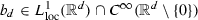
In Figure 2 it is shown how our revised version of Zhikov’s checkerboard example looks for $d=2$. The picture shows the function $u_2$, the (2, 1)-component of $A_2$ and a possible exponent p. The picture should be compared to the one of Figure 1. There are two main differences. First, our version is rotated by $45^\circ$ counterclockwise. Second, there is an additional area, where $u_2=0$. This fact will be very useful later. Note that on the shaded region of $u_2$, resp. $A_2$, we have , which allows us later a freedom in the choice of variable on the shaded region.

Fig. 2

Revised Checkerboard Example

Another difference to the example of Zhikov is the improved regularity away from the singularity at zero.

Proposition 2

There holds

• (a) ,

• (b) ,

• (c) .

Moreover, the following estimates hold

In particular, .

Proof

It is easy to see that and . Moreover, $u_d$ and $A_d$ have the ACL property (absolutely continuous on almost every line parallel to the coordinate axes). Now, the estimates for , are also straightforward. They imply immediately that . This proves the claim. $\square$

For all  we have

again, since $A_d$ is skew-symmetric. Thus,

(1)

This is a crucial property of $b_d$, since it implies that $b_d$ is orthogonal to the gradients of smooth functions. This will allow us later to separate $u_d$ from the smooth functions. Therefore, we call $b_d$ also separating vector field.

It follows from (1) and the regularity of $b_d$ that

(2)

Another important feature of $u_d$ and $b_d$ is the following proposition on the boundary integral that we would obtain it if we were allowed to use partial integration on $\int _\Omega b_d \cdot \nabla u_d\,dx$ (we are not, since $b_d \notin W^{1,1}(\Omega )$).

Proposition 3

Let $\Omega = (-1,1)^d$ with $d \ge 2$. Then

$$\begin{aligned} \int _{\partial \Omega } (b_d \cdot \nu ) u_d\,dS = 1. \end{aligned}$$

For a better understanding we show in Figure 3 the values for $b_2 u_2$ that we need in Proposition 3.

Fig. 3

Boundary values of $b_2 u_2$ used for $\int _{\partial \Omega } (b_2 \cdot \nu )u_2 \,dx =1$

Before we get to the proof we need the following lemma.

Lemma 4

There holds $(\bar{x} \mapsto b_d(\bar{x},1)) \in C^\infty _0((-1,1)^{d-1})$ and

Proof

Let . Then and

Let us define as

Then by the definition of $A_d$ we get

Thus, by the theorem of Gauß

using that $\sigma _{d-1}$ is the surface area of the $d-1$-dimensional sphere. This proves the claim. $\square$

We can now prove Proposition 3.

Proof of Proposition 3

Note that $b_d=0$ on $\partial \Omega$ except for the sets . On these sets $u_d$ takes the values $\pm \frac{1}{2}$ and $\nu = \pm e_d$. Moreover, $b_d\cdot e_d$ is even with respect to $x_d$. Thus,

$$\begin{aligned} \int _{\partial \Omega } (b_d \cdot \nu ) u_d\,dS = \int _{(-1,1)^{d-1}} b_d(\bar{x},1) \cdot e_d\,d\bar{x} = 1 \end{aligned}$$

using Lemma 4. $\square$

2.2 Cantor Sets

In the Zhikov’s example the contact set ${\mathfrak S}$ consists just of one point, the origin, which has dimension zero. For our new examples we want to use contact sets of higher, fractal dimension. For this reason we start with the definition of a few fractal Cantor sets that we need later.

We begin with the one dimensional generalized Cantor set $\mathfrak {C}_\lambda$ with $\lambda \in (0,\frac{1}{2})$, which is also known as the (1-2$\lambda$)-middle Cantor set. We start with the interval $\mathfrak {C}_{\lambda ,0} := [-\frac{1}{2},\frac{1}{2}]$. Then we define $\mathfrak {C}_{\lambda ,k+1}$ inductively by removing the (open) middle $1-2\lambda$ parts from $\mathfrak {C}_{\lambda ,k}$. We set $\mathfrak {C}_\lambda := \cap _{k \ge 1} \mathfrak {C}_{\lambda ,k}$. The corresponding Cantor measure $\mu _\lambda$ (also Cantor distribution) is then defined as the weak limit of the measures . The factor $(2 \lambda )^{-k}$ is chosen such that $\mu _{\lambda ,k}([-\frac{1}{2},\frac{1}{2}])=1= \mu ([-\frac{1}{2},\frac{1}{2}])$. Thus, and . The fractal dimension (Hausdorff dimension) of $\mathfrak {C}_\lambda$ is , i.e. .

We will also need the m-dimensional Cantor sets $\mathfrak {C}_\lambda ^m$ and its distribution $\mu ^m_\lambda$, which are just the Cartesian products of $\mathfrak {C}_\lambda$ and $\mu _\lambda$. Its fractal dimension is . Note that $\mathfrak {C}_\lambda ^m = \cap _{k \ge 1} \mathfrak {C}_{\lambda ,k}^m$.

Fig. 4

Construction of Generalized Cantor Set $\mathfrak {C}_{\frac{1}{3}}$

In the construction of our fractal examples we need a smooth approximation of the indicator function , where . This is the purpose of the following lemma.

Lemma 5

Let $\lambda \in (0,\frac{1}{2})$, $1 \le m \le d$ and let . We use the notation . Let $\frac{1}{4} \le \tau _1 < \tau _2 \le 4$ and $\tau _2-\tau _1 \ge \frac{1}{4}$. Then there exists  such that

• (a) .

• (b) .

In particular, $\rho =1$ on  and $\rho =0$ on .

Proof

Let $\tau := \frac{\tau _2-\tau _1}{2}$. The function would satisfy (a) but not the smoothness requirement. Therefore, we need to mollify this function depending on the -value. For this let denote a standard mollifier, i.e. , $\psi _1\ge 0$, $\int \psi _1\,dx=1$, $\psi _1 \in C_0^\infty (B^d_1(0))$ and $\psi _t(x) = t^{-d}\psi (x/t)$.

The factor $\frac{1}{100}$ in the scaling of the mollifier is chosen so small such that the smeared version of the jump set stays inside . This proves (a). Now, the standard estimate implies (b). It is obvious that . Moreover, since $\rho =0$ on it follows that $\rho$ is also $C^\infty$ at . This proves that . $\square$

The following two lemmas provide further technical estimates that are used later to determine the integrability of our fractal examples. Further ${\mathfrak D}$ will denote the Hausdorff dimension for the fractal set being considered.

Lemma 6

Let $\lambda \in (0,\frac{1}{2})$, $1\le m \le d$ and . We use the notation . Then we have the following properties:

• (a) For every ball $B^m_r(\bar{x})$ there holds .

• (b) For all $r>0$ there holds .

• (c) For all $\tau \in (0,4]$ there holds

  

Proof

Choose  such that $\lambda ^{k+1}< r < \lambda ^k$. Let $A_1, \dots , A_{2^{mk}}$ denote the connected components of $\mathfrak {C}^m_{\lambda ,k}$.

We begin with (b). We estimate

using $2^m = \lambda ^{-{\mathfrak D}}$. This proves (b).

Let us prove (a). If $d(\bar{x}, \mathfrak {C}^m_\lambda )>r$, then $\mu ^m_\lambda (B^m_r(\bar{x}))=0$. This explains the indicator function in (a). Clearly,

$$\begin{aligned} \mu ^m_\lambda (B^m_r(\bar{x}))=\sum _{l=1}^{2^{mk}} \mu ^m_\lambda (B^m_r(\bar{x}) \cap A_l). \end{aligned}$$

By the construction of $\mathfrak {C}^m_{\lambda ,k}$ the sets $A_j$ are pairwise disjoint translates of $(0,\lambda ^k)^m$. So the number of indices l such that the intersection $B^m_r(\bar{x}) \cap A_l$ is nonempty does not exceed $2^m$. Thus

$$\begin{aligned} \mu ^m_\lambda (B^m_r(\bar{x}))\le 2^m\,\mu _\lambda ^m(A_1) = 2^m\, 2^{-mk} = 2^m\, \lambda ^{k {\mathfrak D}} \lesssim r^{{\mathfrak D}} \end{aligned}$$

using again $2^m = \lambda ^{-{\mathfrak D}}$ and $\lambda ^k\le r\lambda ^{-1}$. This finishes the proof of (a).

Let us prove (c). Note that

Now, the claim follows by an application of (a) with . $\square$

The following lemma will be useful to determine later the integrability of our fractal examples.

Lemma 7

Let $\lambda \in (0,\frac{1}{2})$, $1\le m \le d$ and

We use the notation . Then

• (a) for all $0< \beta \le d$.

• (b) for all $0< \beta \le d-{\mathfrak D}$.

Proof

Let $\beta >0$. We begin with (a). Let and $\gamma >0$. If , then . Thus,

This proves (a).

Now, let and $\gamma >0$. If , then . Thus, with Lemma 6 we get

This proves (b). $\square$

Remark 8

Note that integrability exponents $\frac{d}{\beta }$ and $\frac{d-{\mathfrak D}}{\beta }$ in Lemma 7 are sharp. In particular, and with $\Omega = (-1,1)^d$.

2.3 Construction of Fractal Examples

We can now construct our fractal examples, namely the functions u and b. The fractal contact set ${\mathfrak S}$ will in our examples be a subset of  or . By we denote its Hausdorff dimension. In particular, we split  into .

We will provide some pictures after the formal definition.

Definition 9

(Fractal Examples) Let $\Omega := (-1,1)^d$ with $d\ge 2$. Let $u_d,A_d,b_d,$ be as Definition 1. Let $1< p_0 < \infty$. We define u, A, b on $\overline{\Omega }$ distinguishing three cases:

• (a) (Matching the dimension; Zhikov) $p_0=d$:

  Let $u:= u_d$, $A := A_d$, $b := b_d$, and .

• (b) (Sub-dimensional) $1<p_0<d$:

  Let and , where $\lambda \in (0,\frac{1}{2})$ is chosen such that $p_0 = d - {\mathfrak D}$. Let be such that (using Lemma 5)

  • (i) .

  • (ii) .

  We define

  

• (c) (Super-dimensional) $p_0 > d$:

  Let and , where $\lambda \in (0,\frac{1}{2})$ is chosen such that $p_0 = \frac{d-{\mathfrak D}}{1-{\mathfrak D}}$. Let be such that (using Lemma 5)

  • (i) .

  • (ii) .

  We define

  

Remark 10

We will use the functions u, b from the Definition 9 with the exponent $p_0$ later to construct a variable exponent $p\,:\, (-1,1)^d \rightarrow (1,\infty )$ with saddle point value $p_0$ that provides a Lavrentiev gap, see Subsection 4.1. This explains that we use $p_0$ as a parameter to label our fractal examples. Another reason is that $\nabla u$ is in the Marcinkiewicz (weak Lebesgue) space $L^{p_0,\infty }(\Omega )$ and $b \in L^{p_0',\infty }(\Omega )$, see Corollary 16 and Remark 17.

Remark 11

The function $\rho$ in part (b) of Definition 9 plays the same role as $\theta (|x_d|/|{\bar{x}}|)$ in Definition 1, and in part (c) it plays the same role as $\theta (|{\bar{x}}|/|x_d|)$ in Definition 1. If we set formally $\mathfrak {C}_\lambda ^{d-1}=\{0\}^{d-1}$, $\mu _\lambda ^{d-1}=\delta _0^{d-1}$ in (b), then $\rho = \theta (|x_d|/|{\bar{x}}| )$ has the required properties (i), (ii), and the functions u, A, b defined in (b) become $u_d,A_d,b_d$. Similarly, if we set $\mathfrak {C}_\lambda =\{0\}$, $\mu _\lambda = \delta _0$ in (c), then we can take $\rho =\theta (|{\bar{x}}|/|x_d|)$ and the functions u, A, b defined in (c) again become $u_d,A_d,b_d$.

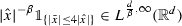
Let us provide a few pictures for the 2D case to illustrate our fractal examples from Definition 9. Using the $\frac{1}{3}$-Cantor set $\mathfrak {C}^1_{\frac{1}{3}}$ we provide in Figure 5, resp. Figure 6, the sub-dimensional, resp. super-dimensional case. The case of matching the dimension is already considered in Figure 1. The left picture shows the values of u. The right picture shows the component $A_{2,1}$ of the skew-symmetric A. The vertical and horizontal patterns indicate that the function is almost linear along those lines.

Fig. 5

Sub-dimensional case: function u and the component $A_{2,1}$ for $d=2$, $p_0=2-{\mathfrak D}$ and . The lines indicate smooth almost linear extensions

Fig. 6

Super-dimensional case: functions u and $A_{2,1}$ for $d=2$, $p_0=\frac{d-{\mathfrak D}}{1-{\mathfrak D}}$ and . The lines indicate smooth almost linear extensions

Remark 12

The use of the skew-symmetric A allows us to avoid the language of differential forms:

• (a) For $d=2$ we can rewrite A as

  $$\begin{aligned} A&= \begin{pmatrix} 0 &{} -v \\ v &{} 0 \end{pmatrix} \end{aligned}$$

  with . Then . Thus, becomes the well known , compare (2) and Proposition 18.

• (b) If $d=3$ we can rewrite A as

  $$\begin{aligned} A&:= \begin{pmatrix} 0 &{} v_3 &{} -v_2 \\ -v_3 &{} 0 &{} v_1 \\ v_2 &{} -v_1 &{} 0 \end{pmatrix} \end{aligned}$$

  with . Then . Thus, becomes the well known . Hence, for $d=3$ we could also work with v and instead of A and . Compare also (2) and Proposition 18.

Remark 13

If we use Remark 12 (b) to find v with then $(x_1,x_2) \mapsto v(x_1,x_2,x_3)$ is just a smooth version of the so called Rankine vortex. It has a central core of radius , where the velocity increases linearly, surrounded by a free vortex, where the velocity drops off from the center like $\frac{1}{r}$ with .

2.4 Properties of the Fractal Examples

Let us derive a few useful properties of u, A and b.

Proposition 14

For $1<p_0<\infty$ let u, A, b be as is Definition 9. Then

• (a) $u \in L^\infty (\Omega ) \cap W^{1,1}(\Omega ) \cap C^\infty (\overline{\Omega } \setminus {\mathfrak S})$,

• (b) $A \in W^{1,1}(\Omega ) \cap C^\infty (\overline{\Omega } \setminus {\mathfrak S})$,

• (c) $b \in L^1(\Omega ) \cap C^\infty (\overline{\Omega } \setminus {\mathfrak S})$.

Proof

The case $p_0=d$ follows from Proposition 2. We continue with the sub-dimensional case $1<p_0 < d$. It is easy to see that $u \in C^\infty (\overline{\Omega } \setminus {\mathfrak S}) \cap L^\infty (\Omega )$. Since and , it follows from the definition by convolution that $A \in C^\infty (\overline{\Omega } \setminus {\mathfrak S})$, so also $b \in C^\infty (\overline{\Omega } \setminus {\mathfrak S})$. It also follows that $A \in W^{1,1}(\Omega )$ and $b \in L^1(\Omega )$. The case $p_0>d$ is similar. $\square$

Proposition 15

For $1<p_0<\infty$ let u, A, b be as is Definition 9.

• (a) If $p_0=d$, then

  

  If $1< p_0 < d$, then

  

  If $p_0>d$, then

  

• (b) a.e. in $\Omega$.

Proof

We begin with (a). The case $p_0=d$ follows directly from Proposition 2. We continue with the sub-dimensional case $1<p_0 < d$. It follows from the properties of $\rho$ that

If follows from

$$\begin{aligned} b&= (\mu ^{d-1}_\lambda \times \delta _0) * b_d, \end{aligned}$$

Proposition 2 and Lemma 6 that

This proves the sub-dimensional case.

If remains to prove the super-dimensional case $p_0 > d$. It follows from the properties of $\rho$ that

If follows from

$$\begin{aligned} \nabla u&= (\delta _0^{d-1} \times \mu _\lambda ) * \nabla u_d, \end{aligned}$$

Proposition 2 and Lemma 6 that

This proves the super-dimensional case and concludes (a).

The estimates in (a) immediately imply that the support of $\nabla u$ and b only overlaps at ${\mathfrak S}$, which is a null set. This proves (b). $\square$

The following corollary clarifies the role of $p_0$ in Definition 9.

Corollary 16

For $1<p_0<\infty$ let u, b be as in Definition 9. Then $\nabla u \in L^{p_0,\infty }(\Omega )$, $b \in L^{p_0',\infty }(\Omega )$.

Proof

The proof is an immediate consequence of Lemma 7 in combination with Proposition 15 (a). For this recall that we have $p_0=d$ for matching the dimension, $p_0=d-{\mathfrak D}$ in the sub-dimensional case and $p_0 = \frac{d-{\mathfrak D}}{1-{\mathfrak D}}$ in the super-dimensional case. We apply Lemma 7 for $m=d-1$ and for $m=1$ to cover all cases. $\square$

Remark 17

The integrability exponents of $\nabla u$ and b are sharp. In particular, $\nabla u \notin L^{p_0}(\Omega )$ and $b \notin L^{p_0'}(\Omega )$. This can be shown with the help of Remark 8.

The following proposition (counterpart of (1) and (2)) shows that b is divergence free in the sense of distributions.

Proposition 18

For all $w \in C^\infty _0(\Omega )$ we have

$$\begin{aligned} \int _\Omega b \cdot \nabla w \,dx = 0, \end{aligned}$$

i.e. in $\Omega$ in the distributional sense. Moreover, in $\Omega \setminus {\mathfrak S}$ in the classical sense.

Proof

We get by partial integration

since A is anti-symmetric. It follows that in the distributional sense. Since by Proposition 14 we have $b \in C^\infty (\overline{\Omega } \setminus {\mathfrak S})$, it follows that in $\Omega \setminus {\mathfrak S}$ in the classical sense. $\square$

Proposition 19

For $1<p_0<\infty$ let u, A, b be as is Definition 9. Then

$$\begin{aligned} \int _{\partial \Omega } (b \cdot \nu ) u\,dS = 1. \end{aligned}$$

Proof

The case $p_0=d$ is already contained in Proposition 3.

Let us continue with the sub-dimensional case $1< p_0 < d$. Note that $b=0$ on $\partial \Omega$ except on the sets . On these sets u takes the values $\pm \frac{1}{2}$ and $\nu = \pm e_d$. Moreover, $b\cdot e_d$ is even with respect to $x_d$. Thus,

(3)

using the first part of Lemma 4. By definition of b we have

This, (3), and Lemma 4 imply

This proves the sub-dimensional case.

For the super-dimensional case $p_0 > d$ the proof is the same as in Proposition 3. Note that $b=0$ on $\partial \Omega$ except on the sets . On these sets u takes the values $\pm \frac{1}{2}$ and $\nu = \pm e_d$. Moreover, $b\cdot e_d$ is even with respect to $x_d$ and $\mathrm {supp}\, (b(\cdot ,1)) \subset B= B^{d-1}_{1/3}(0)\subset \mathbb {R}^{d-1}$. Thus,

$$\begin{aligned} \int _{\partial \Omega } (b \cdot \nu ) u\,dS = \int _{(-1,1)^{d-1}} b(\bar{x},1) \cdot e_d\,d\bar{x} = \int _{B} \frac{1}{ \sigma _{d-1}}\mathrm {div}_{{\bar{x}}}\, (\rho ({\bar{x}},1) |{\bar{x}}|^{1-d}{\bar{x}}) \,d\bar{x} =\\ = \int _{\partial B}\frac{1}{ \sigma _{d-1}}\rho ({\bar{x}},1) |\bar{x}|^{1-d}{\bar{x}}\cdot {{\bar{\nu }}} \, dS = \int _{\partial B} \frac{1}{\sigma _{d-1}} |{\bar{x}}|^{2-d} dS =1. \end{aligned}$$

Here we used that $\rho =1$ on $\partial B$, and ${\bar{\nu }}$ is the outward unit normal to $\partial B$ in $\mathbb {R}^{d-1}$. This proves the super-dimensional case.

$\square$

We also need localized version of u, A and b.

Definition 20

For $1<p_0<\infty$ let u, A, b be as is Definition 9. Let $\eta \in C^\infty _0(\Omega )$ with and . Then we define

Proposition 21

For $1<p_0<\infty$ with the notation of Definition 20 we have

• (a) $u^\circ , A^\circ , b^\circ \in C^\infty (\overline{\Omega } \setminus {\mathfrak S})$ and .

• (b) $u^\partial , A^\partial , b^\partial \in C_0^\infty (\overline{\Omega } \setminus {\mathfrak S})$.

Proof

The claim follows immediately from the definition, and Proposition 14. $\square$

Proposition 22

For all $w \in C^\infty (\Omega )$ we have

$$\begin{aligned} \int _\Omega b^\circ \cdot \nabla w \,dx = 0. \end{aligned}$$

In particular, in $\Omega$ in the distributional sense. Moreover, in $\Omega \setminus {\mathfrak S}$ in the classical sense.

Proof

We get by partial integration

since $\eta$ vanishes on $\partial \Omega$ and A is anti-symmetric. It follows that in the distributional sense. Since by Proposition 21 we have $b^\circ \in C^\infty (\overline{\Omega } \setminus {\mathfrak S})$, it follows that in $\Omega \setminus {\mathfrak S}$ in the classical sense. $\square$

3 Important Consequences

Zhikov used the functions $u_2$ and $b_2$ in order to derive the Lavrentiev gap, $H\ne W$ and the different notions of ${p(\cdot )}$-harmonic functions. We show in this section that also our fractal examples display these phenomena. In this section we will do this in quite general form and apply it to specific examples in Section 4.

3.1 Energy and Generalized Orlicz Spaces

In this section we introduce the necessary function spaces, the so called generalized Orlicz and Orlicz–Sobolev spaces.

We assume that  is a domain of finite measure¹. Later in our applications we will only use $\Omega = (-1,1)^d$.

We say that  is an Orlicz function if is convex, left-continuous, , and . The conjugate Orlicz function  is defined by

In particular, .

In the following we assume that $\phi \,:\, \Omega \times [0,\infty ) \rightarrow [0,\infty ]$ is a generalized Orlicz function, i.e. $\phi (x, \cdot )$ is an Orlicz function for every $x \in \Omega$ and $\phi (\cdot ,t)$ is measurable for every $t\ge 0$. We define the conjugate function $\phi ^*$ pointwise, i.e. $\phi ^*(x,\cdot ) := (\phi (x,\cdot ))^*$.

We further assume the following additional properties:

• (a) We assume that $\phi$ satisfies the $\Delta _2$-condition, i.e. there exists $c \ge 2$ such that for all $x \in \Omega$ and all $t\ge 0$

  $$\begin{aligned} \phi (x,2t)&\le c\, \phi (x,t). \end{aligned}$$

  (4)

• (b) We assume that $\phi$ satisfies the $\nabla _2$-condition, i.e. $\phi ^*$ satisfies the $\Delta _2$-condition. As a consequence, there exist $s>1$ and $c> 0$ such that for all $x\in \Omega$, $t\ge 0$ and $\gamma \in [0,1]$ there holds

  $$\begin{aligned} \phi (x,\gamma t) \le c\,\gamma ^s \,\phi (x,t). \end{aligned}$$

  (5)

• (c) We assume that $\phi$ and $\phi ^*$ are proper, i.e. for every $t\ge 0$ there holds $\int _\Omega \phi (x,t)\,dx< \infty$ and $\int _\Omega \phi ^*(x,t)\,dx < \infty$.

Let $L^0(\Omega )$ denote the set of measurable function on $\Omega$ and denote the space of locally integrable functions. We define the generalized Orlicz norm by

Then generalized Orlicz space $L^{{\phi (\cdot )}}(\Omega )$ is defined as the set of all measurable functions with finite generalized Orlicz norm,

For example the generalized Orlicz function $\phi (x,t) = t^p$ generates the usual Lebesgue space $L^p(\Omega )$.

The $\Delta _2$-condition of $\phi$ and $\phi ^*$ ensures that our space is uniformly convex. The condition that $\phi$ and $\phi ^*$ are proper ensure that and . Thus $L^{{\phi (\cdot )}}(\Omega )$ and $L^{{\phi ^*(\cdot )}}(\Omega )$ are Banach spaces.

We define the generalized Orlicz–Sobolev space $W^{1,{\phi (\cdot )}}$ as

with the norm

In general smooth functions are not dense in $W^{1,{\phi (\cdot )}}(\Omega )$. Therefore, we define $H^{1,{\phi (\cdot )}}(\Omega )$ as

$$\begin{aligned} H^{1,{\phi (\cdot )}}(\Omega )&:= \big (\text {closure of }~C^\infty (\Omega ) \cap W^{1,{\phi (\cdot )}}(\Omega )\text { in }~W^{1,{\phi (\cdot )}}(\Omega )\big ). \end{aligned}$$

See [5] and [10] for further properties of these spaces.

We also introduce the corresponding spaces with zero boundary values as

with same norm as in $W^{1,\phi (\cdot )}(\Omega )$. And the corresponding space of smooth functions is defined as

$$\begin{aligned} H_0^{1,{\phi (\cdot )}}(\Omega )&:= \big (\text {closure of } C^\infty _0(\Omega ) \cap W^{1,{\phi (\cdot )}}(\Omega ) \text { in } W^{1,{\phi (\cdot )}}(\Omega )\big ). \end{aligned}$$

The space $W_0^{1,{\phi (\cdot )}}(\Omega )$ are exactly those function, which can be extended by zero to  functions.

Let us define our energy  by

In the language of function spaces ${\mathcal {F}}$ is a semi-modular on $W^{1,{\phi (\cdot )}}(\Omega )$ and a modular on $W^{1,{\phi (\cdot )}}_0(\Omega )$.

3.2 H $\ne$ W and $\hbox {H}_0 \ne$ $\hbox {W}_0$

In this section we show how to use the function u and the vector b from Definition 9 to give examples for $W^{1,{\phi (\cdot )}}(\Omega ) \ne H^{1,{\phi (\cdot )}}(\Omega )$ and for $W_0^{1,{\phi (\cdot )}}(\Omega ) \ne H^{1,{\phi (\cdot )}}_0(\Omega )$. In this section, we need the following assumption:

Assumption 23

Let $u,u^\circ , u^\partial ,b, b^\circ ,b^\partial$ be as in Section 2, i.e. Proposition 14, 15, 19 and 21 hold. Let $\phi$ be such that $u \in W^{1,{\phi (\cdot )}}(\Omega )$ and $b \in L^{{\phi ^*(\cdot )}}(\Omega )$.

For all $w \in W^{1,{\phi (\cdot )}}(\Omega )$ we define the continuous functionals

$$\begin{aligned} \begin{aligned} {\mathcal {S}}(w)&:= \int _\Omega b \cdot \nabla w \,dx, \\ {\mathcal {S}}^\circ (w)&:= \int _\Omega b^\circ \cdot \nabla w \,dx, \\ {\mathcal {S}}^\partial (w)&:= \int _\Omega b ^\partial \cdot \nabla w \,dx. \end{aligned} \end{aligned}$$

(6)

This is well defined, since $b, b^\circ , b^\partial \in L^{{\phi ^*(\cdot )}}(\Omega )$.

Proposition 24

For all $w \in H^{1,{\phi (\cdot )}}(\Omega )$ we have ${\mathcal {S}}^\circ (w)=0$. Moreover, for all $w \in H^{1,{\phi (\cdot )}}_0(\Omega )$ we have ${\mathcal {S}}(w)=0$.

Proof

Due to Propositions 22 and 18 we have ${\mathcal {S}}^\circ (w)=0$ for $w \in C^\infty (\Omega )$ and ${\mathcal {S}}(w)=0$ for $w \in C^\infty _0(\Omega )$. Now, the claim follows by density. $\square$

Proposition 25

There holds

• (a) ${\mathcal {S}}(u) = 0$, ${\mathcal {S}}(u^\partial ) = 1$ and ${\mathcal {S}}(u^\circ ) =-1$.

• (b) $\mathcal {S}^{\partial }(u) = 1$, $\mathcal {S}^{\partial }(u^\partial ) = 1$ and $\mathcal {S}^{\partial }(u^\circ ) = 0$.

• (c) ${\mathcal {S}}^\circ (u) = -1$, ${\mathcal {S}}^\circ (u^\partial ) = 0$ and ${\mathcal {S}}^\circ (u^\circ ) = -1$.

Proof

Since $b\cdot \nabla u=0$ everywhere, we have ${\mathcal {S}}(u)=0$. Note that the supports of $u^\partial$ and $b^\partial$ are separated from the fractal set and these functions are both smooth, i.e. $u^\partial , b^\partial \in C^\infty _0(\overline{\Omega } \setminus {\mathfrak S})$. Thus, we can use partial integration to get

$$\begin{aligned} {\mathcal {S}}^\partial (u^\partial )&= \int _\Omega b^\partial \cdot \nabla u^\partial \,dx = \int _{\partial \Omega } (b^\partial \cdot \nu ) u^\partial \,ds = \int _{\partial \Omega } (b \cdot \nu ) u\,ds = 1 \end{aligned}$$

using also Proposition 19. Since $u^\partial \in C^\infty _0(\overline{\Omega } \setminus {\mathfrak S})$, $b^\circ \in C^\infty (\overline{\Omega } \setminus {\mathfrak S})$, and on $\Omega \setminus {\mathfrak S}$, we can use partial integration to get

Analogously, we obtain ${\mathcal {S}}^\partial (u^\circ )=0$. Now,

$$\begin{aligned} {\mathcal {S}}^\circ (u^\circ )&= {\mathcal {S}}(u) - {\mathcal {S}}^\partial (u^\partial ) - {\mathcal {S}}^\circ (u^\partial ) - {\mathcal {S}}^\partial (u^\circ ) = 0 - 1 - 0 - 0 = -1. \end{aligned}$$

This proves the claim. $\square$

Due to Propositions 24 and 25 the functionals ${\mathcal {S}}$ and ${\mathcal {S}}^\circ$ are called separating functionals and the functions b and $b^\circ$ are called separating vector fields.

We come to the main result of this subsection.

Theorem 26

(H $\ne$ W) Under the assumption 23 there holds

• (a) $u^\circ \in W^{1,{\phi (\cdot )}}(\Omega ) \setminus H^{1,{\phi (\cdot )}}(\Omega )$.

• (b) $u^\circ \in W_0^{1,{\phi (\cdot )}}(\Omega ) \setminus H_0^{1,{\phi (\cdot )}}(\Omega )$.

Proof

Recall that $u^\circ \in W^{1,{\phi (\cdot )}}_0(\Omega ) \subset W^{1,{\phi (\cdot )}}(\Omega )$. Due to Proposition 24 we know that ${\mathcal {S}}^\circ =0$ on $H^{1,{\phi (\cdot )}}(\Omega )$ and therefore also on $H_0^{1,{\phi (\cdot )}}(\Omega )$. However, ${\mathcal {S}}^\circ (u^\circ ) = -1$ by Proposition 25. This proves $u^\circ \notin H^{1,{\phi (\cdot )}}(\Omega )$ and $u^\circ \notin H^{1,{\phi (\cdot )}}_0(\Omega )$. This proves the claim. $\square$

3.3 Lavrentiev Gap

In this section we show how to use the function u and the vector field b from Definition 9 for the Lavrentiev gap. In this section, we need the following assumption:

Assumption 27

Let $u,u^\circ , u^\partial ,b, b^\circ ,b^\partial$ as in Section 2, i.e. Proposition 14, 15, 19 and 21 hold. Let $\phi$ be such that $u \in W^{1,{\phi (\cdot )}}(\Omega )$ and $b \in L^{{\phi ^*(\cdot )}}(\Omega )$. Also recall, that $\phi ^*$ satisfies the $\Delta _2$-condition.

From the $\Delta _2$-condition of $\phi ^*$, see (5), it follows that

(7)

We come to the main result of this subsection.

Theorem 28

(Lavrentiev gap) Under the assumptions 27 the functional

$$\begin{aligned} {\mathcal {G}} := {\mathcal {F}} + {\mathcal {S}}^\circ \end{aligned}$$

with ${\mathcal {S}}^\circ$ defined in (6) has a Lavrentiev gap, i.e.

$$\begin{aligned} \inf {\mathcal {G}}(W^{1,{\phi (\cdot )}}_0(\Omega )) < \inf {\mathcal {G}}(H^{1,{\phi (\cdot )}}_0(\Omega ))=0. \end{aligned}$$

Proof

Due to Proposition 24 we have ${\mathcal {G}} = {\mathcal {F}}$ on $H^{1,{\phi (\cdot )}}_0(\Omega )$, which implies that $\inf {\mathcal {G}}(H^{1,{\phi (\cdot )}}_0(\Omega ))= 0$. However, for $t >0$ we have

$$\begin{aligned} {\mathcal {G}}(t u^\circ )&= {\mathcal {F}}(t u^\circ ) + t\, {\mathcal {S}}^\circ (u^\circ ) = t\, \bigg ( \frac{{\mathcal {F}}(tu^\circ )}{t} - 1 \bigg ) \end{aligned}$$

using ${\mathcal {S}}^\circ (u^\circ )=-1$ by Proposition 25. Since $\lim _{t\rightarrow 0} \frac{{\mathcal {F}}(t u^\circ )}{t} = 0$ by (7), the right-hand side becomes negative for small $t>0$. Thus $\inf {\mathcal {G}}(W^{1,{\phi (\cdot )}}_0(\Omega )) < 0$. $\square$

3.4 H-harmonic $\ne$ W-harmonic

In this section we show that the spaces $W^{1,{\phi (\cdot )}}(\Omega )$ and $H^{1,{\phi (\cdot )}}(\Omega )$ lead to different concepts of ${\phi (\cdot )}$-harmonic functions.

Let us start by introducing spaces with boundary values: for $g \in H^{1,{\phi (\cdot )}}(\Omega )$ we define

$$\begin{aligned} H_g^{1,{\phi (\cdot )}}(\Omega )&:= g + H_0^{1,{\phi (\cdot )}}(\Omega ). \end{aligned}$$

For $g \in W^{1,{\phi (\cdot )}}(\Omega )$ we define

$$\begin{aligned} W_g^{1,{\phi (\cdot )}}(\Omega )&:= g + W_0^{1,{\phi (\cdot )}}(\Omega ). \end{aligned}$$

Since $u^\partial \in W^{1,{\phi (\cdot )}}(\Omega )$, we can define

$$\begin{aligned} h_W&= {\text {arg min}}{\mathcal {F}}\big (W^{1,{\phi (\cdot )}}_{u^\partial }(\Omega )\big ). \end{aligned}$$

Formally, it satisfies the Euler-Lagrange equation (in the weak sense)

where $\phi '(x,t)$ is the derivative with respect to t. However, since also $u^\partial \in H^{1,{\phi (\cdot )}}(\Omega )$, we can define

$$\begin{aligned} h_H&= {\text {arg min}}{\mathcal {F}}\big (H^{1,{\phi (\cdot )}}_g(\Omega )\big ). \end{aligned}$$

Then

If $\phi (x,t)=\frac{1}{2} t^2$, then $\Delta _{\phi (\cdot )}$ is just the standard Laplacian. If $\phi (x,t)=\frac{1}{p} t^p$, then $\Delta _{\phi (\cdot )}$ is the p-Laplacian.

Thus $h_W$ and $h_H$ are both ${\phi (\cdot )}$-harmonic but $h_W$ is ${\phi (\cdot )}$-harmonic in the sense of $W^{1,{\phi (\cdot )}}$ and $h_H$ is ${\phi (\cdot )}$-harmonic with respect to $H^{1,{\phi (\cdot )}}$. Our goal is to provide an example, where these concepts differ. For this we assume the following:

Assumption 29

Let $u,u^\circ , u^\partial ,b, b^\circ ,b^\partial$ as in Section 2, i.e. Proposition 14, 15, 19 and 21 hold. Let $\phi$ be such that $u \in W^{1,{\phi (\cdot )}}(\Omega )$ and $b \in L^{{\phi ^*(\cdot )}}(\Omega )$.

Moreover, assume that there exist $s,t > 0$ such that

$$\begin{aligned} {\mathcal {F}}(tu) + {\mathcal {F}}^*(s b)&< t s, \end{aligned}$$

(8)

where

We come to the main result of this subsection.

Theorem 30

(H-harmonic $\ne$ W-harmonic) Under the Assumption 29 there exists $g \in H^{1,{\phi (\cdot )}}(\Omega )$ such that the ${\phi (\cdot )}$-harmonic functions $h_W$ in the sense of $W^{1,{\phi (\cdot )}}$ and the ${\phi (\cdot )}$-harmonic function $h_H$ in the sense of $H^{1,{\phi (\cdot )}}$ with the same boundary values g differ. In particular, for

$$\begin{aligned} h_W&= {\text {arg min}}{\mathcal {F}}\big (W^{1,{\phi (\cdot )}}_{u^\partial }(\Omega )\big )\\ h_H&= {\text {arg min}}{\mathcal {F}}\big (H^{1,{\phi (\cdot )}}_{u^\partial }(\Omega )\big ) \end{aligned}$$

we have $h_W \ne h_H$ and ${\mathcal {F}}(h_W) < {\mathcal {F}}(h_H)$.

Proof

We define $g := t u^\partial \in H^{1,{\phi (\cdot )}}(\Omega )$, with $t>0$ to be chosen later. Now, let

$$\begin{aligned} w_t&:= {\text {arg min}}{\mathcal {F}}(W^{1,{\phi (\cdot )}}_{tu^\partial }(\Omega )),\\ h_t&:= {\text {arg min}}{\mathcal {F}}(H^{1,{\phi (\cdot )}}_{tu^\partial }(\Omega )). \end{aligned}$$

We have $t u = tu^\partial + tu^\circ \in W_{t u^\partial }^{1,{\phi (\cdot )}}(\Omega )$. Thus,

$$\begin{aligned} {\mathcal {F}}(w_t)&\le {\mathcal {F}}(t u). \end{aligned}$$

(9)

From the other hand, using Young’s inequality, we get for all $s>0$ that

Since $h_t - tu^\partial \in H_0^{1,{\phi (\cdot )}}(\Omega )$, we have ${\mathcal {S}}(h_t - tu^\partial )=0$ by Theorem 24. This and ${\mathcal {S}}(u^\partial )=1$ by Proposition 25 imply

$$\begin{aligned} {\mathcal {F}}(h_t)&= s\,{\mathcal {S}}(t u^\partial ) - {\mathcal {F}}^*(s b) = t s - {\mathcal {F}}^*(s b). \end{aligned}$$

(10)

Combining (9) and (10) we get

$$\begin{aligned} {\mathcal {F}}(h_t) - {\mathcal {F}}(w_t) \ge t s - {\mathcal {F}}(tu) - {\mathcal {F}}^*(s b) \end{aligned}$$

for all $t,s > 0$. By Assumption 8 we can find $t,s>0$ such that the right hand-side of last inequality is positive. For these t, s we have ${\mathcal {F}}(h_t) > {\mathcal {F}}(w_t)$. This proves the claim for $h_H := h_t$ and $h_W := w_t$. $\square$

4 Applications

We will now apply our results to the following three models:

4.1 Variable Exponents

In this section we study the variable exponent model. In particular, we assume that

$$\begin{aligned} \phi (x,t) = \tfrac{1}{p(x)} t^{p(x)}, \end{aligned}$$

where $p\,:\, \Omega \rightarrow (1,\infty )$ is a variable exponent. The corresponding energy is

We abbreviate $W^{1,{p(\cdot )}}(\Omega ) := W^{1,{\phi (\cdot )}}(\Omega )$ and similarly $W^{1,{p(\cdot )}}_0$, $H^{1,{p(\cdot )}}$ and $H^{1,{p(\cdot )}}_0$.

Our main result of the variable exponent model is the following:

Theorem 31

Let $\Omega =(-1,1)^d$. Let $1< p^-< p^+ < \infty$. Then there exists a variable exponent $p\,:\, \Omega \rightarrow [p^-,p^+]$ such that

• (a) $H^{1,{p(\cdot )}}(\Omega ) \ne W^{1,{p(\cdot )}}(\Omega )$ and $H_0^{1,{p(\cdot )}}(\Omega ) \ne W_0^{1,{p(\cdot )}}(\Omega )$.

• (b) There exists a linear, continuous functional  such that functional ${\mathcal {G}} := {\mathcal {F}} + {\mathcal {S}}^\circ$ has a Lavrentiev gap, i.e.

  $$\begin{aligned} \inf {\mathcal {G}}\big (W^{1,{p(\cdot )}}_0(\Omega ) \big )&< \inf {\mathcal {G}}\big (H^{1,{p(\cdot )}}_0(\Omega )\big ) =0. \end{aligned}$$

• (c) The notions of ${p(\cdot )}$-harmonic functions with respect to $W^{1,{p(\cdot )}}$ and $H^{1,{p(\cdot )}}$ differ.

Proof

Choose $p_0$ with $p^-< p_0 < p^+$. Now, let u, b be as in Definition 9 and ${\mathcal {S}}^\circ$ as in (6). We begin with the definition of the variable exponent p.

• (a) (Matching the dimension; Zhikov) $p_0=d$: Define

  

• (b) (Sub-dimensional) $1<p_0<d$: Define

  

• (c) (Super-dimensional) $p_0 > d$: Define

  

In particular, it follows from Proposition 15 that

(11)

Thus, with Corollary 16 and $p^-< p_0 < p^+$ we obtain

This proves $u \in W^{1,{p(\cdot )}}(\Omega )$ and $b \in L^{p'(\cdot )}(\Omega )$. This proves the validity of Assumption 23.

Since $1< p^- \le p \le p^+ < \infty$, it follows that $\phi$ and $\phi ^*$ satisfy the $\Delta _2$ condition. Thus Assumption 27 also holds.

Using (11) we obtain for all $s,t>0$

$$\begin{aligned} {\mathcal {F}}(tu) + {\mathcal {F}}^*(sb)&= t^{p^-} {\mathcal {F}}(u) + s^{(p^+)'} {\mathcal {F}}^*(b)\\&= \tfrac{1}{p_0} t^{p_0} \big ( t^{p^--p_0} p_0 {\mathcal {F}}(u) \big ) + \tfrac{1}{p_0'} s^{p_0'} \big ( s^{(p^+)'-p_0'} p_0' {\mathcal {F}}^*(b) \big ). \end{aligned}$$

Now, fix $s:= t^{p_0}-1$. Then for suitable large t (and therefore large s) we obtain

$$\begin{aligned} {\mathcal {F}}(tu) + {\mathcal {F}}^*(sb)&\le \tfrac{1}{p_0} t^{p_0} \cdot \tfrac{1}{2} + \tfrac{1}{p_0'} s^{p_0'} \tfrac{1}{2} = \tfrac{1}{2} ts < ts. \end{aligned}$$

This proves Assumption 29.

Overall, we have constructed u, b, and p such that the Assumptions 23, 27 and 29 holds. Now, the claim follows from the results of Theorem 26, 28 and 30 of Section 3. $\square$

The exponent in Theorem 31 was discontinuous at the singular set ${\mathfrak S}$. The following result shows that it is also possible to construct a uniformly continuous exponent with the same phenomena. However, this exponent is not $\log$-Hölder continuous, since this would imply the $H^{1,{p(\cdot )}}(\Omega )=W^{1,{p(\cdot )}}(\Omega )$ by means of convolution, see [22] and [5, Section 4.6].

Theorem 32

Let $\Omega =(-1,1)^d$ with $d \ge 2$. Let $1< p_0 < \infty$. Let ${\mathfrak S}$ (the fractal contact set) be as in Definition 9. Then there exists a uniformly continuous variable exponent p with saddle points on ${\mathfrak S}$ and $p=p_0$ on ${\mathfrak S}$ and

• (a) $H^{1,{p(\cdot )}}(\Omega ) \ne W^{1,{p(\cdot )}}(\Omega )$ and $H_0^{1,{p(\cdot )}}(\Omega ) \ne W_0^{1,{p(\cdot )}}(\Omega )$.

• (b) There exists a linear, continuous functional  such that functional ${\mathcal {G}} := {\mathcal {F}} + {\mathcal {S}}^\circ$ has a Lavrentiev gap, i.e.

  $$\begin{aligned} \inf {\mathcal {G}}\big (W^{1,{p(\cdot )}}_0(\Omega ) \big )&< \inf {\mathcal {G}}\big (H^{1,{p(\cdot )}}_0(\Omega )\big ) =0. \end{aligned}$$

• (c) The notions of ${p(\cdot )}$-harmonic functions with respect to $W^{1,{p(\cdot )}}$ and $H^{1,{p(\cdot )}}$ differ.

Proof

The proof is similar to the one of Theorem 31. So we only point out the difference. Let u, b be as in Definition 9 and ${\mathcal {S}}^\circ$ as in (6). We have to show that $\nabla u \in L^{p(\cdot )}(\Omega )$ and $b \in L^{p'(\cdot )}(\Omega )$ and to verify Assumption 29.

Let $\sigma (t) := \frac{1}{(\log (e+1/t))^\kappa }$ with $0<\kappa < 1$. Then for any $c_1 > 0$ there holds

(12)

• (a) We begin with the case of matching the dimension $p_0=d$. Let $\theta _p \in C^\infty _0((0,\infty ))$ be such that and and define

  

  Then p is uniformly continuous with modulus of continuity $\sigma$. It follows by Proposition 15,  (12) and $p_0=d$ that

  

  (13)

  and

  

  This proves $\nabla u \in L^{p(\cdot )}(\Omega )$ and $b \in L^{p'(\cdot )}(\Omega )$.

• (b) We continue with the sub-dimensional case $1< p_0 < d$. Let be such that (using Lemma 5)

  • (a) .

  • (b) .

  and define

  

  Then p is uniformly continuous with modulus of continuity $\sigma$. It follows by Proposition 15, Lemma 6, (12) and $p_0=d-{\mathfrak D}$ that

  

  (14)

  and

  

  This proves $\nabla u \in L^{p(\cdot )}(\Omega )$ and $b \in L^{p'(\cdot )}(\Omega )$.

• (c) Let us turn to the super-dimensional case $p_0 > d$. Let be such that (using Lemma 5)

  • (a) .

  • (b)

  and define

  

  Then p is uniformly continuous with modulus of continuity $\sigma$. It follows by Proposition 15, Lemma 6, (12), $p_0=\frac{d-{\mathfrak D}}{1-{\mathfrak D}}$ and $1-{\mathfrak D}= \frac{d-1}{p_0-1}$ that

  

  and

  

  This proves $\nabla u \in L^{p(\cdot )}(\Omega )$ and $b \in L^{p'(\cdot )}(\Omega )$.

We have proved $\nabla u \in L^{p(\cdot )}(\Omega )$ and $b \in L^{p'(\cdot )}(\Omega )$ for all $1< p_0 < \infty$. We are now going to verify Assumption 29. We restrict ourselves to the sub-dimensional case, since the other cases are similar.

We will show that

$$\begin{aligned} {\mathcal {F}}(tu) + {\mathcal {F}}^*(sb) \le \tfrac{1}{2} st \end{aligned}$$

for suitable large s, t.

Let $s,t > 1$ (to be fixed later). For $\epsilon >0$ we define the $\epsilon$-neighborhood of ${\mathfrak S}$ by

Now, with the definition of $p^\pm$ and (13) we obtain

Since , we can choose $\epsilon _0>0$ small such that $\text {I},\text {III} < \tfrac{1}{4}$ for all $\epsilon \in (0, \epsilon _0)$. Then choose $t_0,s_0$ large (depending on $\epsilon _0$) such that  $\text {II},\text {IV} < \tfrac{1}{4}$ for all $t \ge t_0$ and $s\ge s_0$. Thus, we obtain

$$\begin{aligned} {\mathcal {F}}(tu ) + {\mathcal {F}}^*(sb)&\le \tfrac{1}{2} \Big ( \tfrac{1}{p_0}t^{p_0} + \tfrac{1}{p_0'}s^{p_0'} \Big ) \end{aligned}$$

for all $t\ge t_0$ and $s \ge s_0$. Now, the choice $s:=t^{p_0-1}$ implies for large t that

$$\begin{aligned} {\mathcal {F}}(tu ) + {\mathcal {F}}^*(sb)&\le \tfrac{1}{2} st < st. \end{aligned}$$

This proves Assumption 29.

Overall, we have constructed u, b, and p such that the Assumptions 23, 27 and 29 hold. Now, the claim follows from the results from Theorem 26, 28 and 30 of Section 3. $\square$

Theorem 31 and Theorem 32 show in particular that the dimensional threshold is not important for the presence of the Lavrentiev gap and the non-density of smooth functions.

Remark 33

At this point we also have to mention the work of [13], since it seemingly contradicts our results. The authors claimed that if $p^- \ge d$ [13, Theorem 4.1] or if $2 \le p^- < d$ and $p^+ < \frac{d p^-}{d-p^-}$ [13, Theorem 4.2]. Our examples show that both claims are wrong.²

4.2 Double Phase Potential

In this section we study the double phase model. In particular, we assume that

$$\begin{aligned} \phi (x,t) = \tfrac{1}{p} t^p + a(x) \tfrac{1}{q} t^q = \tfrac{1}{p} t^p + \tfrac{1}{q} (\omega (x)t)^q, \end{aligned}$$

where $1< p < q$ with a weights $a,\omega \ge 0$. The corresponding energy is

(15)

Let us denote by $C^k$ the space of k-times differentiable functions. Moreover, denote by $C^{k+\beta }$ for $\beta \in (0,1)$ and the space of functions from $C^k$ whose k-th derivatives are $\beta$-Hölder continuous.

Theorem 34

Let $\Omega =(-1,1)^d$ with $d\ge 2$. Let $p>1$ and with $\alpha >0$. Then there exists $a \in C^{\alpha }(\overline{\Omega })$ such that

• (a) $H^{1,{\phi (\cdot )}}(\Omega ) \ne W^{1,{\phi (\cdot )}}(\Omega )$ and $H_0^{1,{\phi (\cdot )}}(\Omega ) \ne W_0^{1,{\phi (\cdot )}}(\Omega )$.

• (b) There exists a linear, continuous functional  such that functional ${\mathcal {G}} := {\mathcal {F}} + {\mathcal {S}}^\circ$ has a Lavrentiev gap, i.e.

  $$\begin{aligned} \inf {\mathcal {G}}\big (W^{1,{\phi (\cdot )}}_0(\Omega ) \big )&< \inf {\mathcal {G}}\big (H^{1,{\phi (\cdot )}}_0(\Omega )\big ) =0. \end{aligned}$$

• (c) The notions of ${p(\cdot )}$-harmonic functions with respect to $W^{1,\phi (\cdot )}$ and $H^{1,\phi (\cdot )}$ differ.

Proof

Since and is continuous in p, we can choose $p_0>p$ such that . In particular, $p< p_0 < q$.

Now, let u, b be as in Definition 9 and ${\mathcal {S}}^\circ$ as in (6). We begin with the definition of our weight a(x), resp. $\omega (x) = (a(x))^{\frac{1}{q}}$.

• (a) (Matching the dimension; Zhikov) $p_0=d$: Let $\theta _a \in C^\infty _0((0,\infty ))$ be such that and . We define

  

• (b) (Sub-dimensional) $1<p_0<d$: Let be such that (using Lemma 5)

  • (a) .

  • (b) .

  We define

  

• (c) (Super-dimensional) $p_0 > d$: Let be such that (using Lemma 5)

  • (a) .

  • (b)

  We define

  

Then is follows easily by the properties of $\rho _a$ that $a \in C^\alpha (\overline{\Omega })$. Moreover, in the sub-dimensional case and the case of matching the dimension we have

(16a)

while in the super-dimensional case we have

(16b)

Thus, it follows from $p < p_0$ and Corollary 16 that

In the following let x be such that $b(x)>0$. Then for $p_0 \le d$ and for $p_0 > d$. Since $\phi (x,t) \ge a(x) \frac{1}{q} t^q = \frac{1}{q} (\omega (x) t)^q$, it follows that $\phi ^*(x,t)\le \frac{1}{q'} (t/\omega (x))^{q'} = \frac{1}{q'} a(x)^{-\frac{1}{q-1}} t^{p'}=: \psi (x,t)$. This implies

(17a)

and

(17b)

We claim that  for some $r>1$. To prove this we distinguish three cases using Proposition 15.

• (a) (Matching the dimension; Zhikov) $p_0=d$:

  

  Thus, by Lemma 7 we have with $r:= \frac{d(q-1)}{\alpha +(d-1)q}$. Now, $r>1$ is equivalent to $q > d+\alpha = p_0 + \alpha$, which is true by choice of $p_0$.

• (b) (Sub-dimensional) $1<p_0=d - {\mathfrak D}<d$:

  

  Thus, by Lemma 7 we have with $r:= \frac{(d-{\mathfrak D})(q-1)}{\alpha +(d-{\mathfrak D}-1)q}$. Now, $r>1$ is equivalent to $q > d-{\mathfrak D}+ \alpha = p_0 + \alpha$, which is true by choice of $p_0$.

• (c) (Super-dimensional) $p_0= \frac{d-{\mathfrak D}}{1-{\mathfrak D}} > d$:

  

  Thus, by Lemma 7 (applied to $m=1$) we have with $r:= \frac{(d-{\mathfrak D})(q-1)}{\alpha +(d-1)q}$. Now, $r>1$ is equivalent to $q > \frac{\alpha +d-{\mathfrak D}}{1-{\mathfrak D}} = \frac{\alpha }{1-{\mathfrak D}} + p_0$. Since $p_0 =\frac{d-{\mathfrak D}}{1-{\mathfrak D}}$, we have $1-{\mathfrak D}= \frac{d-1}{p_0-1}$. Thus, $r>1$ is equivalent to $q> p_0 + \alpha \frac{d-1}{p_0-1}$, which is true by choice of $p_0$.

We have proved that some $r>1$, which proves . Due to (17) this implies and therefore $b \in L^{\phi ^*(\cdot )}(\Omega )$. Overall, we have verified Assumption 23.

Since $p,q \in (1,\infty )$, it follows that $\phi$ and $\phi ^*$ satisfy the $\Delta _2$ condition. Thus Assumption 27 also holds.

Let $s,t>0$ (to be fixed later). By (16) we have

$$\begin{aligned} {\mathcal {F}}(tu)&= t^p {\mathcal {F}}(u). \end{aligned}$$

Moreover, by (17) we have

Thus, we have

Since $p<p_0 < q$, we get

Now, fix $s:= t^{p_0-1}$. Then for suitable large t (and therefore large s) we obtain

$$\begin{aligned} {\mathcal {F}}(tu) + {\mathcal {F}}^*(sb)&\le \tfrac{1}{p_0} t^{p_0} \cdot \tfrac{1}{2} + \tfrac{1}{p_0'} s^{p_0'} \tfrac{1}{2} = \tfrac{1}{2} ts < ts, \end{aligned}$$

where we have used $p<p_0$ and $q' < p_0'$. This proves Assumption 29.

Overall, we have constructed u, b, and p such that the Assumptions 23, 27 and 29 holds. Now, the claim follows from the results from Theorem 26, 28 and 30 of Section 3. $\square$

Remark 35

Theorem 34 shows that the dimensional threshold is not important for the presence of the Lavrentiev gap and the non-density of smooth functions. (Recall that the previous examples needed $p<d< d+\alpha < p$ crossing the dimension.)

Since we have overcome the dimensional threshold, it might be surprising that we obtain different conditions on p and q for $p\le d$ and $p>d$. Therefore, let us explain in the following that our conditions are sharp.

Consider first the case $p \le d$. In this case we get Lavrentiev gap for $q> p+\alpha$. Now, it has been shown in [2] that if h is a bounded local minimizer of ${\mathcal {F}}$ and $q \le p+\alpha$, then h is automatically in . Since it follows that $h \in H^{1,{\phi (\cdot )}}(\Omega )$ and there is no Lavrentiev gap. This shows that our condition $q>p+\alpha$ is sharp. The boundeness of the minimizer is a reasonable assumption due to the maximum principle. Also note that our function u is also bounded. This is reflected by the fact that functions in $W^{1,{\phi (\cdot )}}(\Omega )$ can always be approximated by $L^\infty (\Omega ) \cap W^{1,{\phi (\cdot )}}(\Omega )$ functions by means of truncation.

Now, consider the case $p > d$. In this case it has been shown in [1, Theorem 1.4] that if h is a minimizer of ${\mathcal {F}}$, $h \in C^{0,\gamma }(\overline{\Omega })$ and $q \le p +\frac{\alpha }{1-\gamma }$, then h is automatically in $W^{1,q}(\Omega )$. Again implies that $h \in H^{1,{\phi (\cdot )}}(\Omega )$ and there is no Lavrentiev gap. Now, in our example we constructed a function $u \in {\mathcal {C}}^{0,{\mathfrak D}}(\overline{\Omega })$ with ${\mathfrak D}= \frac{p_0-d}{p_0-1}$. Thus, we can compare our condition $q > p + \alpha \frac{p-1}{d-1}$ for the Lavrentiev gap with $q \le p+\frac{\alpha }{1-\gamma }$ for $\gamma := {\mathfrak D}$ for the absence of the Lavrentiev gap. Now, $p+ \frac{\alpha }{1-{\mathfrak D}} = p + \alpha \frac{p_0-1}{d-1}$. Since $p_0$ can be chosen close to p this shows that our condition $q > p + \alpha \frac{p-1}{d-1}$ is sharp.

Remark 36

Fonseca, Malý and Mingione studied in [9] the size of possible singular sets of minimizer of the double phase potential (15). For $1< p< d< d+\alpha< q < \infty$ they constructed a weight such that the singular set has Hausdorff dimension larger than $d-p-\epsilon$.

Let us compare this to our result. Since $p<d$, we can choose $p_0 = p+\delta$ with $\delta >0$ small. Thus, our function u has a singular set of Hausdorff dimension ${\mathcal {D}}= d-p_0= d-p-\delta$. In particular, we obtain a singular set of the same size. Note however, that our function u is not a minimizer yet, but we expect that we can use u as a competitor to find a minimizer with a singular set of same Hausdorff dimension. We will work on this question in a future project. Using out method we hope to overcome the dimensional threshold $p< d< d+\alpha < q$ from [9].

4.3 Weighted p-Energy

In this section we study the model with weighted p-energy. In particular, we assume that

$$\begin{aligned} \phi (x,t)&= \tfrac{1}{p} a(x) t^p =\tfrac{1}{p} (\omega (x) t)^p \end{aligned}$$

where $1< p < \infty$ and weights $a, \omega \ge 0$ (almost everywhere). The corresponding energy is

Definition 37

The weight a(x) belongs to the Muckenhoupt class $A_p$ if

where the supremum is taken over all cubes Q.

Our main result of the weighted p-energy is the following:

Theorem 38

Let $\Omega =(-1,1)^d$ with $d\ge 2$ and $1< p < \infty$. Then there exist weights $a^-$ and $a^+$ of Muckenhoupt class $A_p$ and another weight a with $a^- \le a \le a^+$ such that the following holds:

• (a) $H^{1,{\phi (\cdot )}}(\Omega ) \ne W^{1,{\phi (\cdot )}}(\Omega )$ and $H_0^{1,{\phi (\cdot )}}(\Omega ) \ne W_0^{1,{\phi (\cdot )}}(\Omega )$.

• (b) There exists a linear, continuous functional  such that ${\mathcal {G}} := {\mathcal {F}} + {\mathcal {S}}^\circ$ has a Lavrentiev gap, i.e.

  $$\begin{aligned} \inf {\mathcal {G}}\big (W^{1,{\phi (\cdot )}}_0(\Omega ) \big )&< \inf {\mathcal {G}}\big ((H^{1,{\phi (\cdot )}}_0(\Omega )\big ) =0. \end{aligned}$$

• (c) The notions of ${\phi (\cdot )}$-harmonic functions with respect to $W^{1,{\phi (\cdot )}}$ and $H^{1,{\phi (\cdot )}}$ differ.

It is possible to choose either a or $\frac{1}{a}$ bounded.

Proof

Let $\alpha ,\beta , \gamma$ be such that

$$\begin{aligned} -\frac{1}{p}< \alpha< \gamma< \beta < \frac{1}{p'}. \end{aligned}$$

If $\alpha ,\beta \ge 0$, then a will be bounded. If $\alpha , \beta \le 0$, then $\frac{1}{a}$ will be bounded

If $\gamma = 1-\frac{d}{p}$, let $p_0 := d$. If $\gamma \in (1-\frac{d}{p},\frac{1}{p'})$, choose $p_0 \in (1,d)$ (and hence $p_0 = d-{\mathfrak D}$) such that $\gamma = 1-\frac{p_0}{p}$. If $\gamma \in (-\frac{d-1}{p},1 -\frac{d}{p})$ choose $p_0>d$ (and hence $p_0 = \frac{d-{\mathfrak D}}{1-{\mathfrak D}}$) such that $\gamma = \frac{d-1}{p_0-1}(1-\frac{p_0}{p})= \frac{d-1}{p} \frac{p-p_0}{p_0-1}$. Moreover, let $\epsilon >0$ be another parameter. To obtain (c), we have to choose $\epsilon >0$ later small.

Now, let u, b be as in Definition 9 and ${\mathcal {S}}^\circ$ as in (6). For our construction and proof we distinguish the three cases $p_0=d$, $p_0 < d$ and $p_0>d$.

• (a) We begin with the case of matching the dimension $p_0=d$. Let $\theta _a \in C^\infty _0((0,\infty ))$ be such that and . We define

  

  We can assume that $\epsilon \le d^{\frac{\beta -\alpha }{2}}$, so that $\omega ^- \le \omega \le \omega ^+$. The weights $\omega ^-$ and $\omega ^+$ are of Muckenhoupt class $A_p$, since $\alpha , \beta \in (-\frac{1}{p}, \frac{1}{p'})$. It follows by Proposition 15 that

  

  (18)

  and

  

  Thus, by Lemma 7 we have with $r=\frac{d}{(1-\beta )p}>1$ using $\beta > \gamma =1-\frac{d}{p}$. This proves $\nabla u \in L^{\phi (\cdot )}(\Omega )$. Moreover, by Lemma 7 we have with $s=\frac{d}{(\alpha +d-1)p'}>1$ using $\alpha < \gamma =1-\frac{d}{p}$. This proves $b \in L^{\phi ^*(\cdot )}(\Omega )$.

• (b) We continue with the sub-dimensional case $1< p_0 < d$. Let be such that (using Lemma 5)

  • (a) .

  • (b) .

  and define

  

  We can assume that $\epsilon \le d^{\frac{\beta -\alpha }{2}}$, so that $\omega ^- \le \omega \le \omega ^+$. The weights $\omega ^-$ and $\omega ^+$ are of Muckenhoupt class $A_p$, since $\alpha , \beta \in (-\frac{1}{p}, \frac{1}{p'})$. It follows by Proposition 15 that

  

  (19)

  and

  

  Thus, by Lemma 7 we have with $r=\frac{d-{\mathfrak D}}{(1-\beta )p}>1$ using $\beta > \gamma = 1 - \frac{d-{\mathfrak D}}{p} = 1 - \frac{p_0}{p}$. This proves $\nabla u \in L^{\phi (\cdot )}(\Omega )$. Moreover, by Lemma 7 we have with $s=\frac{d-{\mathfrak D}}{d-1-{\mathfrak D}+\alpha }>1$ using $\alpha < \gamma = 1 - \frac{d-{\mathfrak D}}{p} = 1 - \frac{p_0}{p}$. This proves $b \in L^{\phi ^*(\cdot )}(\Omega )$.

• (c) Let us turn to the super-dimensional case $p_0 > d$. Let be such that (using Lemma 5)

  • (a) .

  • (b)

  and define

  

  The weights $\omega ^-$ and $\omega ^+$ are of Muckenhoupt class $A_p$, since $\alpha , \beta \in (-\frac{d-1}{p}, \frac{d-1}{p'})$. It follows by Proposition 15 that

  

  and

  

  Thus, by Lemma 7 we have with $r=\frac{d-{\mathfrak D}}{(1-{\mathfrak D}-\alpha )p}>1$ using $\beta > \gamma = 1-{\mathfrak D}-\frac{d-{\mathfrak D}}{p} = \frac{d-1}{p_0-1}(1-\frac{p_0}{p})$. This proves $\nabla u \in L^{\phi (\cdot )}(\Omega )$. Moreover, by Lemma 7 we have with $s=\frac{d-{\mathfrak D}}{(d-1+\beta )p'}>1$ using $\beta < \gamma = 1-{\mathfrak D}-\frac{d-{\mathfrak D}}{p} = \frac{d-1}{p_0-1}(1-\frac{p_0}{p})$. This proves $b \in L^{\phi ^*(\cdot )}(\Omega )$.

Now $1<p<\infty$ ensures that $\phi$ and $\phi ^*$ satisfy the $\Delta _2$-condition.

Overall, we have constructed u, b, and p such that the Assumptions 23 and 27 hold.

We are now going to verify Assumption 29. This will be the step, where we have to choose $\epsilon >0$ small enough. It suffices to prove Assumption 29 in the case of $p_0 < d$. (The other cases are completely analogous.)

Let $s,t>0$ (to be fixed later). By (19) we have

Moreover, by (17) we have

Thus, there exist $c_1,c_2>0$ such that

$$\begin{aligned} {\mathcal {F}}(tu) + {\mathcal {F}}^*(sb)&\le c_1 (\epsilon t)^p + c_2 s^{p'}. \end{aligned}$$

Now, the choice $t:=1$, $s:= \epsilon ^{p-1}$ and $\epsilon = (\frac{1}{2 (c_1 +c_2)})^{\frac{1}{p}}$ implies

$$\begin{aligned} {\mathcal {F}}(tu) + {\mathcal {F}}^*(sb)&\le \epsilon ^p\, (c_1+c_2) = \tfrac{1}{2} ts < ts. \end{aligned}$$

This proves Assumption 29.

Overall, we have constructed u, b, and p such that the Assumptions 23, 27 and 29 holds. Now, the claim follows from the results from Theorem 26, 28 and 30 of Section 3. $\square$

Remark 39

Note, that Zhikov has also provided in [20, Section 5.3] another example for $H^{1,{\phi (\cdot )}}(\Omega ) \ne W^{1,{\phi (\cdot )}}(\Omega )$ for the model of the weighted p-energy for $p=2$. He was interested in an example, where the weight is bounded. Since, the checker board example does not work in this case, he constructed an example using fractals. For this he split the domain $\Omega$ into two parts $\Omega _1$ and $\Omega _0$ separated by another part ${\mathcal {N}}$ consisting of a Cantor-necklace, see Figure 7. He then constructed a weight $a\in L^{\infty }(\Omega )$ with $\frac{1}{a} \in L^1(\Omega )$ and a function $u \in (L^\infty (\Omega ) \cap W^{1,{\phi (\cdot )}}(\Omega )) \setminus H^{1,{\phi (\cdot )}}(\Omega )$ with $u = 0$ on $\Omega _0$ and $u=1$ on $\Omega _1$. The weight was chosen such that it is integrable on each block of the necklace and scaled by the size on the smaller blocks. So the weight becomes smaller on smaller blocks. His example is contained in the class of possible weights from Theorem 38.

Fig. 7

Zhikov’s fractal barrier

We would like to thank the reviewer for careful reading of our paper, valuable remarks and suggestions.

References

Baroni, P., Colombo, M., Mingione, G.: Regularity for general functionals with double phase. Calc. Var. Partial Differ. Equ. 57(2), 48 (2018)
Colombo, M., Mingione, G.: Bounded minimisers of double phase variational integrals. Arch. Ration. Mech. Anal. 218(1), 219–273 (2015)
Cruz-Uribe, D.V., Fiorenza, A.: Variable Lebesgue Spaces. Applied and Numerical Harmonic Analysis. Foundations and Harmonic Analysis. Birkhäuser/Springer, Heidelberg (2013)
Diening, L.: Maximal function on generalized Lebesgue spaces \(L^{p(\cdot )}\). Math. Inequal. Appl. 7(2), 245–253 (2004)
Diening, L., Harjulehto, P., Hästö, P., Růžička, M.: Lebesgue and Sobolev Spaces with Variable Exponents, volume 2017 of Lecture Notes in Mathematics, 1st edn. Springer (2011)
Diening, L., Hästo, P., Nekvinda, A.: Open problems in variable exponent Lebesgue and Sobolev spaces. In: FSDONA04 Proceedings, pp. 38–52. 01 (2004)
Edmunds, D.E., Rákosník, J.: Density of smooth functions in \(W^{k, p(x)}(\Omega )\). Proc. R. Soc. Lond. Ser. A 437(1899), 229–236 (1992)
Esposito, L., Leonetti, F., Mingione, G.: Sharp regularity for functionals with \((p, q)\) growth. J. Differ. Equ. 204(1), 5–55 (2004)
Fonseca, I., Malý, J., Mingione, G.: Scalar minimizers with fractal singular sets. Arch. Ration. Mech. Anal. 172(2), 295–307 (2004)
Harjulehto, P., Hästö, P.: Generalized Orlicz Spaces. Springer, Cham (2019)
Hästö, P.A.: Counter-examples of regularity in variable exponent Sobolev spaces. In: The \(p\)-Harmonic Equation and Recent Advances in Analysis, volume 370 of Contemporary Mathematics, pp. 133–143. Amer. Math. Soc., Providence, RI (2005)
Kokilashvili, V., Meskhi, A., Rafeiro, H., Samko, S.: Integral Operators in Non-standard Function Spaces. Vol. 1, volume 248 of Operator Theory: Advances and Applications. Birkhäuser/Springer, [Cham], Variable exponent Lebesgue and amalgam spaces (2016)
Kostopoulos, T., Yannakakis, N.: Density of smooth functions in variable exponent Sobolev spaces. Nonlinear Anal. 127, 196–205 (2015)
Lavrentiev, M.: Sur quelques problemes du calcul des variations. Ann. Math. Pura Appl. 4, 107–124 (1926)
Manià, B.: Sopra un esempio di Lavrentieff. Bull. Un. Mat. Ital. 13, 147–153 (1934)
Marcellini, P.: Regularity of minimizers of integrals of the calculus of variations with nonstandard growth conditions. Arch. Ration. Mech. Anal. 105(3), 267–284 (1989)
Surnachev, M.D.: Density of smooth functions in weighted Sobolev spaces with variable exponent. Dokl. Math. 89(2), 146–150 (2014)
Zhikov, V.V., Surnachev, M.D.: On density of smooth functions in weighted Sobolev spaces with variable exponents. St Petersb. Math. J. 27, 415–436 (2016)
Zhikov, V.V.: Averaging of functionals of the calculus of variations and elasticity theory. Izv. Akad. Nauk SSSR Ser. Mat. 50(4), 675–710 (1986)
Zhikov, V.V.: On weighted Sobolev spaces. Mat. Sb. 189(8), 27–58 (1998)
Zhikov, V. V.: On the density of smooth functions in Sobolev–Orlicz spaces. Zap. Nauchn. Sem. S.-Peterburg. Otdel. Mat. Inst. Steklov. (POMI). 310(Kraev. Zadachi Mat. Fiz. i Smezh. Vopr. Teor. Funkts. 35 [34]):67–81 (2004)
Zhikov, V.V.: On Lavrentiev’s phenomenon. Russ. J. Math. Phys. 3(2), 249–269 (1995)
Funding
Open Access funding provided by Projekt DEAL.
Author information
Authors and Affiliations
Corresponding author
Additional information
Communicated by T. Riviere.
Dedicated to Vasiliĭ Vasil’evich Zhikov.
Publisher's Note
Springer Nature remains neutral with regard to jurisdictional claims in published maps and institutional affiliations.
Anna Kh.Balci and Lars Diening thank the German Research Foundation (DFG) for the support through the CRC 1283. The research of Mikhail Surnachev was supported by the Russian Science Foundation under grant 19-71-30004. Mikhail Surnachev acknowledges warm hospitality of Bielefeld University.
Rights and permissions
Open Access This article is licensed under a Creative Commons Attribution 4.0 International License, which permits use, sharing, adaptation, distribution and reproduction in any medium or format, as long as you give appropriate credit to the original author(s) and the source, provide a link to the Creative Commons licence, and indicate if changes were made. The images or other third party material in this article are included in the article’s Creative Commons licence, unless indicated otherwise in a credit line to the material. If material is not included in the article’s Creative Commons licence and your intended use is not permitted by statutory regulation or exceeds the permitted use, you will need to obtain permission directly from the copyright holder. To view a copy of this licence, visit http://creativecommons.org/licenses/by/4.0/.
About this article
Cite this article
Balci, A.K., Diening, L. & Surnachev, M. New Examples on Lavrentiev Gap Using Fractals. Calc. Var. 59, 180 (2020). https://doi.org/10.1007/s00526-020-01818-1
Received:
Accepted:
Published:
DOI: https://doi.org/10.1007/s00526-020-01818-1