Disease eradication on large industrial farms

Abstract

Many modern farms exhibit all-in-all-out dynamics in which entire cohorts of livestock are removed from a farm before a new cohort is introduced. This industrialization has enabled diseases to spread rapidly within farms. Here we look at one such example, Marek’s disease. Marek’s disease is an economically important disease of poultry. The disease is transmitted indirectly, enabling the spread of disease between cohorts of chickens who have never come into physical contact. We develop a model which allows us to track the transmission of disease within a barn and between subsequent cohorts of chickens occupying the barn. It is described by a system of impulsive differential equations. We determine the conditions that lead to disease eradication. For a given level of transmission we find that disease eradication is possible if the cohort length is short enough and/or the cohort size is small enough. Marek’s disease can also be eradicated from a farm if the cleaning effort between cohorts is large enough. Importantly complete cleaning is not required for eradication and the threshold cleaning effort needed declines as both cohort duration and size decrease.

Appendices

Appendix: A

Lemma 1

The solution to the difference Eq. 7 is:

$$\begin{aligned} I_m=\frac{I_0N(ae^{N\beta T})^m}{N+I_0(e^{N\beta T}-1) \sum _{k=0}^{m-1}(ae^{N\beta T})^k} \end{aligned}$$

(10)

Proof

The proof is by induction.

Suppose $m=1$

From (10)

$$\begin{aligned} I_1&=\frac{I_0N(ae^{N\beta T})^1}{N+I_0(e^{N\beta T}-1) \sum _{k=0}^{0}(ae^{N\beta T})^k} \\&=\frac{I_0Nae^{N\beta T}}{N-I_0(1-e^{N\beta T})} \end{aligned}$$

Now considering the difference Equation (7), if we let $m=0$, we also obtain

$$\begin{aligned} I_{1}=\frac{I_0Nae^{N\beta T}}{N-I_0(1-e^{N\beta T})}. \end{aligned}$$

Now assume the $m^{th}$ case is true. Then from Equation (10) the $(m+1)^{th}$ case is

$$\begin{aligned} I_{m+1}&=\frac{I_0N(ae^{N\beta T})^{m+1}}{N+I_0(e^{N\beta T}-1) \sum _{k=0}^{m}(ae^{N\beta T})^k} \\&=\frac{I_0N(ae^{N\beta T})^m(ae^{N\beta T})}{I_0(ae^{N\beta T})^m(e^{N\beta T}-1)+N+I_0(e^{N\beta T}-1) \sum _{k=0}^{m-1}(ae^{N\beta T})^k} \\&=\frac{I_0N(ae^{N\beta T})^m(ae^{N\beta T})}{I_0(ae^{N\beta T})^m(e^{N\beta T}-1)+\frac{I_0(ae^{N\beta T})^mN}{I_m}} \quad \text {from}\;(10) \\&=\frac{Nae^{N\beta T}}{(e^{N\beta T}-1)+\frac{N}{I_m}} \quad \text {By dividing each term by}\;I_0(ae^{N\beta T})^m \\ I_{m+1}&=\frac{I_mNae^{N\beta T}}{N-I_m(1-e^{N\beta T})} \end{aligned}$$

which is precisely Equation (7), concluding the proof. $\square$

Theorem 1

The nontrivial fixed point

$$\begin{aligned} I^*=\frac{N(1-ae^{N\beta T})}{1-e^{N\beta T}} \end{aligned}$$

of the difference Equation (7) is globally stable if $ae^{N\beta T}> 1$. If $ae^{N\beta T}<1$ then $I^*=0$ will be globally stable.

Proof

From Lemma 1 we have

$$\begin{aligned} I_m=\frac{I_0N(ae^{N\beta T})^m}{N+I_0(e^{N\beta T}-1) \sum _{k=0}^{m-1}(ae^{N\beta T})^k} \end{aligned}$$

which we can simplify to

$$\begin{aligned} I_m=\frac{I_0(ae^{N\beta T})^mN}{N+I_0(e^{N\beta T}-1) \left( \frac{1-(ae^{N\beta T})^{m}}{1-(ae^{N\beta T})} \right) } \end{aligned}$$

Assume $ae^{N\beta T}<1$. Then

$$\begin{aligned} \lim _{m\rightarrow \infty }I_m&=\frac{0}{N+(I_0e^{N\beta T}-I_0) \left( \frac{1}{1-(ae^{N\beta T})} \right) }\\&=0 \end{aligned}$$

Now suppose $ae^{N\beta T}>1$.

$$\begin{aligned} \lim _{m\rightarrow \infty }I_m=\lim _{m\rightarrow \infty }\frac{I_0(ae^{N\beta T})^mN}{N+(I_0e^{N\beta T}-I_0) \left( \frac{1-(ae^{N\beta T})^{m}}{1-(ae^{N\beta T})} \right) } \end{aligned}$$

We can divide every term by $(ae^{N\beta T})^m$

$$\begin{aligned} \lim _{m\rightarrow \infty }I_m=\lim _{m\rightarrow \infty }\frac{I_0N}{\frac{N}{(ae^{N\beta T})^m}-I_0\frac{(1-e^{N\beta T})}{1-ae^{N\beta T}}\frac{1-(ae^{N\beta T})^m}{(ae^{N\beta T})^m}} \end{aligned}$$

note that :

$$\begin{aligned} \lim _{m\rightarrow \infty }\frac{1-(ae^{N\beta T})^m}{(ae^{N\beta T})^m}=\lim _{m\rightarrow \infty }\frac{\frac{1}{(ae^{N\beta T})^m}-1}{1}=-1 \end{aligned}$$

therefore

$$\begin{aligned} \lim _{m\rightarrow \infty } I_m=\frac{N(1-ae^{N\beta T})}{1-e^{N\beta T}}=I^* \end{aligned}$$

which is our non-trivial fixed point. $\square$

Appendix: B

Let $v>0$ in system (4). If we assume that $0<v<<1$ then we can express the solutions of the differential equations in (4) as a power series in v. If we substitute the first two terms of the power series, $S(t)\approx S_0(t)+vS_1(t)$ and $I(t) \approx I_0(t)+vI_1(t)$, into the differential Equations (4) and collect terms with equal powers of v while neglecting higher powers of v, we arrive at two systems of differential Eqs. (11) and (12).

$$\begin{aligned} \frac{dS_0(t)}{dt}= & {} -\beta S_0(t)I_0(t), \quad S_0(0)=s_0 \nonumber \\ \frac{dI_0(t)}{dt}= & {} \beta S_0(t)I_0(t), \quad I_0(0)=i_0 \end{aligned}$$

(11)

with $s_0+i_0=N$ and

$$\begin{aligned} \frac{dS_1(t)}{dt}= & {} -\beta S_0(t)I_1(t)-\beta S_1(t)I_0(t), \quad S_1(0)=0 \nonumber \\ \frac{dI_1(t)}{dt}= & {} \beta S_0(t)I_1(t)+\beta S_1(t)I_0(t)-I_0(t), \quad I_1(0)=0. \end{aligned}$$

(12)

Notice (11) is exactly the system of differential equations from Sect. (3.1) with solutions,

$$\begin{aligned} S_0(t)= & {} \frac{Ns_0e^{-N\beta t}}{N-s_0(1-e^{-N\beta t})} \\ I_0(t)= & {} \frac{Ni_0e^{N\beta t}}{N-i_0(1-e^{N\beta t})}. \end{aligned}$$

If we add the two differential equations in (12)

$$\begin{aligned} \frac{dS_1}{dt}+\frac{dI_1}{dt}= & {} -I_0 \\ dS_1+dI_1= & {} -I_0dt \end{aligned}$$

and integrate we get an expression for the sum $S_1(t)+I_1(t).$

$$\begin{aligned} S_1(t)+I_1(t)=\frac{1}{\beta }\ln (N)-\frac{1}{\beta }\ln (N-i_0(1-e^{N\beta t})). \end{aligned}$$

(13)

If we substitute (13) and $S_0(t)+I_0(t)=N$ into the linear approximations $S\approx S_0+vS_1$ and $I\approx I_0+vI_1$, we get an approximate solution for the sum $S(t)+I(t)$.

$$\begin{aligned} S(t)+I(t)\approx N-v\left( \frac{1}{\beta }\ln (N)-\frac{1}{\beta }\ln (N-i_0(1-e^{N\beta t}))\right) . \end{aligned}$$

(14)

By evaluating (14) at $t=(m+1)T$ where $m=0,1,2,\dots$ with initial condition $I(mT^+)$ and hence $t=T$, we get the approximate sum of the susceptible and infected chickens at the end of the $(m+1)^{th}$ cohort, $S((m+1)T^-)+I((m+1)T^-)$. By substituting both (14) and $I(mT^+)=aI(mT^-)$ into (8) we can eliminate the S(t) terms. Using the same notation as in Sect. (3.1), $I_{m}{:=}I(mT^+)$ and $I_{m+1}{:=}I((m+1)T^+)$, we arrive at:

$$\begin{aligned} I_{m+1}\approx & {} a\left[ -v\left( \frac{1}{\beta }\ln (N)-\frac{1}{\beta } \ln (N-I_m(1-e^{N\beta T}))\right) +\frac{I_{m+1}}{a}\right. \\&\left. +\frac{v}{\beta }\left( \ln \frac{N+v(\frac{1}{\beta }\ln (N)-\frac{1}{\beta }\ln (N-I_m(1-e^{N\beta T})))-\frac{I_{m+1}}{a}}{N-I_m} \right) \right] . \end{aligned}$$

By factoring in the a and solving for $I_{m+1}$ we arrive at an approximate iterative function of the time points directly after impulse for model (5):

$$\begin{aligned} I_{m+1}\approx \frac{aNI_me^{N\beta T}}{N-I_m(1-e^{N\beta T})}+\frac{va}{\beta }\ln \left( \frac{N}{N-I_m(1-e^{N\beta T})} \right) . \end{aligned}$$

(15)

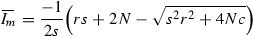
Let $c=aNe^{N\beta T}$, $s=-(1-e^{N\beta T})$, and $r=va/\beta$, where $c>s,r>0$. Making these substitutions, (15) can be rewritten as (16).

$$\begin{aligned} I_{m+1}=f(I_m)=\frac{cI_m}{N+sI_m}+r\ln \left( \frac{N}{N+sI_m} \right) \end{aligned}$$

(16)

The derivative of (16) with respect to $I_m$ is:

$$\begin{aligned} f'(I_m)=\frac{Nc-Nsr-s^2rI_m}{(N+sI_m)^2}. \end{aligned}$$

(17)

and we define ${\varLambda }_2$ to be the value of the derivative (17) evaluated at $I_m=0$.

$$\begin{aligned} {\varLambda }_2=\frac{c-sr}{N}. \end{aligned}$$

Note that if we substitute the constants c, s, and r back into ${\varLambda }_2$ we have:

$$\begin{aligned} {\varLambda }_2=ae^{N\beta T}-\frac{va(e^{N\beta T}-1)}{\beta N}. \end{aligned}$$

Let $g(I_m)=f(I_m)-I_m$. The fixed points of the difference Equation (16) are the roots of $g(I_m)$.

Theorem 2

• 1. If ${\varLambda }_2>1$ the difference Equation (16) has two fixed points ($I_1^*=0$ and $I_2^*>0$).

• 2. If ${\varLambda }_2>1$ The nontrivial fixed point, $I_2^*$, is globally attractive. If ${\varLambda }_2<1$ the fixed point, $I_1^*=0$, is globally attractive.

Proof

• (1) By evaluating (16) at $I_m=0$, it is easy to show that $I_1^*=0$ is a fixed point. For us to conclude that (16) has one and only one other fixed point, we will show that the function $g(I_m)$ has exactly one root with $I_m>0$.

  First note that for $I_2^*>0$ to exist we require $I_m>0$ and from (8) we know that $I_m<N$. Also note that $g(I_m)$ is continuous and differentiable on [0, N], and

  $$\begin{aligned} g(0)=0, \quad g'(0)>0 \quad \text {and} \quad g(N)<0 \end{aligned}$$

  Therefore there exists a number $0<b$ such that $g(b)>0$ and by the Intermediate Value Theorem, there exists at least one number $I_2^*\in [b,N]$ such that $g(I_2^*)=0$.

  By taking the derivative $g'(I_m)$ and setting it to zero we can show that $g(I_m)$ has one nonnegative critical point

  

  when ${\varLambda }_2>1$. $g'(I_m)>0$ for and $g'(I_m)<0$ for . Therefore is a global maximum and .

  Suppose that $g(I_m)$ has at least one other root $I_3^*$, such that $I_2^*<I_3^*<N$. Then by Rolle’s theorem there must exist a number k such that $I_2^*<k<I_3^*$ and $g'(k)=0$. Since is the only critical point and , we have a contradiction. Thus $I_2^*$ is the only nonzero root of $g(I_m)$. Therefore $f(I_m)$ has a single nonzero fixed point when ${\varLambda }_2>1$.

• (2) We can take v sufficiently small such that $f'(I_m)>0$ for $I_m\in [0,N]$ and $f'(I_m)$ is continuous and decreasing.

  From $g(I_m)$ we can see that for $I_m<I_2^*$, $f(I_m)> I_m$. Therefore for $0<I_m<I_2^*$, $f(I_m)$ is monotonically increasing and bounded above by $I_2^*$ and by the Monotone Convergence Theorem converges to the fixed point $I_2^*$. Similarly for $I_2^*<I_m<N$, $f(I_m)$ is monotonically decreasing and bounded below by $I_2^*$ and hence converges to the fixed point $I_2^*$. Therefore the nontrivial fixed point $I_2^*$ is globally attractive when ${\varLambda }_2>1$.

  Suppose ${\varLambda }_2<1$. Then $f(I_m)<I_m$ for all $I_m\in (0,N)$ and $f(I_m)$ is monotonically decreasing and bounded below by $I_1^*=0$. Therefore by the Monotone Convergence Theorem, $f(I_m)$ converges to the fixed point $I_1^*=0$. Hence for ${\varLambda }_2<1$ the fixed point $I_1^*=0$ is globally attractive.$\square$

References

Atkins K, Read AF, Savill N, Renz K, Islam S, Walkden-Brown AFMF, Woolhouse M (2012) Vaccination and reduced cohort duration can drive virulence evolution: Marek’s disease virus and industrial agriculture. Evolution 67:851–860. doi:10.1111/j.1558-5646.2012.01803.x
Benton W, Cover M (1957) The increased incidence of visceral lymphomatosis in broiler and replacement birds. Avian Dis 1(3):320–327
Biggs P, Payne L (1967) Studies on marek’s disease. i. experimental transmission. J Nat Cancer Inst 39(2):267–280
Costello M (2006) Ecology of sea lice parasitic on farmed and wild fish. Trends Parasitol 22(10):475–483
Dawkins M, Donnelly C, Jones T (2004) Chicken welfare is influenced more by housingconditions than by stocking density. Nature 427:342–344
Dunn J, Gimeno I (2013) Current status of Marek’s disease in the United States and worldwide based on a questionnaire survey. Avian Dis 57:483–490
Fanatico A, Owens C, Emmert J (2009) Organic poultry production in the United States: broilers. J Appl Poult Res 18(2):355–366
Grunder A, Gavora J, Spencer J, Turnbull J (1975) Prevention of mareks disease using a filtered air positive pressure house. Poult Sci 54(4):1189–1192
Jones T, Donnelly C, Dawkins M (2005) Environment, well-being, and behavior. Environment and management factors affecting welfare of chickens on comercial farms in the united kingdom and denmark stocked at five densities. Poult Sci 84:1155–1165
Jurajda V, Klimes B (1970) Presence and survival of marek’s disease agent in dust. Avian dis 14(1):88–190
Krkošek M, Lewis M, Volpe J (2005) Transmission dynamics of parasitic sea lice from farm to wild salmon. Proc R Soc Lond B Biol Sci 272(1564):689–696
Lowell A, BN, HT, KJ, SP (2008) “Pseudorabies (Aujeszky’s Disease) and Its Eradication”, tech. rep., USDA
Malone B (2006) Managing built-up litter. In: Proceedings to 2006 Midwest poultry federation conference, St. Paul, MN, 21–23 March 2006
Morrow C, Fehler F (2004) Marek’s disease: a worldwide problem. Marek’s disease, An Evolving Problem, pp 49–61
Müller T, Bätza H, Schlüter H, Conraths F, Mettenleiter T (2003) Eradication of aujeszky’s disease in germany. J Vet Med Ser B 50(5):207–213
Nair V (2005) Evolution of mareks disease-a paradigm for incessant race between the pathogen and the host. Vet J 170(2):175–183
Sheppard A (2004) The structure and economics of broiler production in england. University of Exeter. Centre for Rural Research, vol 59
Witter R (1997) Mareks disease: a worldwide problem. Avian Dis 41(1):149–163
Witter R, Burgoyne G, Burmester B (1968) Survival of marek’s disease agent in litter and droppings. Avian dis 12(3):522–530
Yu X, Zhou Z, Hu D, Zhang Q, Han T, Li X, Gu X, Yuan L, Zhang S, Wang B et al (2014) Pathogenic pseudorabies virus, china, 2012. Emerg Infect Dis 20(1):102
Acknowledgments
The RAPIDD program of the Science & Technology Directorate, Department of Homeland Security, and the Fogarty International Center, National Institutes of Health.
Author information
Authors and Affiliations
Corresponding author