The local fundamental group of a Kawamata log terminal singularity is finite

Abstract

We prove a conjecture of Kollár stating that the local fundamental group of a klt singularity x is finite. In fact, we prove a stronger statement, namely that the fundamental group of the smooth locus of a neighbourhood of x is finite. We call this the regional fundamental group. As the proof goes via a local-to-global induction, we simultaneously confirm finiteness of the orbifold fundamental group of the smooth locus of a weakly Fano pair.

1 Introduction

We work over the field ${{\mathbb {C}}}$ of complex numbers. A log pair is an algebraic variety X together with a boundary divisor $0 \le \varDelta < 1$ of the form $\varDelta =\varDelta '+\varDelta ''$, with $0 \le \varDelta ''$ and $\varDelta '=\sum (1-1/m_i)\varDelta _i$ is a sum of prime divisors $\varDelta _i$, whose coefficients satisfy $m_i \in {{\mathbb {Z}}}_{>1}$.

A Kawamata log terminal or klt singularity is a point $x \in (X,\varDelta )$, such that for a log resolution $f:Y \rightarrow X$, locally around x, the discrepancies $a_i$, namely the coefficients of the exceptional divisors $E_i$ in the formula

$$\begin{aligned} K_Y + f^{-1}_*\varDelta \sim _{{\mathbb {Q}}}f^*(K_X+\varDelta )+\sum a_i E_i \end{aligned}$$

satisfy $a_i > -1$. We call a log pair $(X,\varDelta )$ weakly Fano, if it has only klt singularities and $-(K_X+\varDelta )$ is big and nef. The local fundamental group of a normal singularity $x \in X$ is

$$\begin{aligned} \pi _1^\mathrm{loc}(X,x):=\pi _1(B {\setminus } x) =\pi _1(\mathrm{Link}(x)), \end{aligned}$$

where B is the intersection of X with a small euclidean ball around x and the link $\mathrm{Link}(x)$ is the boundary $\partial B$. It is a deformation retract of $B {\setminus } x$ and so $\pi _1^\mathrm{loc}$ is well defined. The following conjecture is due to Kollár [40, 43].

Conjecture 1

Let $x \in (X,\varDelta )$ be a klt singularity. Then the local fundamental group $\pi _1^\mathrm{loc}(X,x)$ is finite.

In the case of a weakly Fano pair $(X,\varDelta )$, one can consider the smooth locus of X and state the following global conjecture [1, 60].

Conjecture 2

Let $(X,\varDelta )$ be a weakly Fano pair. Then the fundamental group $\pi _1(X_\mathrm{sm})$ of the smooth locus is finite.

This conjecture has been proven for log del Pezzo surfaces [28, 36, 37] and log Fano varieties of high Fano index [60].

We prove generalized versions of both conjectures in the present paper. Firstly, for a log pair $(X,\varDelta )$ with decomposition $\varDelta =\varDelta '+\varDelta ''$ as above, we can consider the complex orbifold $\mathcal {X}=(X,\varDelta ')$, see Sect. 2. Then one can consider the orbifold fundamental group of the smooth locus, denoted by $\pi _1(X_\mathrm{sm},\varDelta ')$. This group is defined to be $\pi _1(X_\mathrm{sm}{\setminus } \mathrm{supp}(\varDelta '))/N$, where N is the normal subgroup generated by the $\gamma _i^{m_i}$, where $\gamma _i$ is a small loop around $\varDelta _i$. Similarly to the global case, in the local setting we can consider the fundamental group $\pi _1(B_\mathrm{sm})=\pi _1(B {\setminus } X_\mathrm{sing})$ of the smooth locus of B, instead of the local fundamental group. We call this group the regional fundamental group and denote it by $\pi _1^\mathrm{reg}(X,x)$. It is also possible to define the orbifold fundamental group of $(B_\mathrm{sm},\left. \varDelta ' \right| _{B_\mathrm{sm}})$, which we denote by $\pi _1^\mathrm{reg}(X,\varDelta ',x)$. Our two main theorems are the following.

Theorem 1

Let $x \in (X,\varDelta '+\varDelta '')$ be a klt singularity. Then the regional fundamental groups $\pi _1^\mathrm{reg}(X,x)$ and $\pi _1^\mathrm{reg}(X,\varDelta ',x)$ are finite.

Theorem 2

Let $(X,\varDelta '+\varDelta '')$ be a weakly Fano pair. Then the orbifold fundamental group $\pi _1(X_\mathrm{sm},\varDelta ')$ of the smooth locus is finite.

Before sketching the structure of the (simultaneous) proof of these theorems, we give a short overview of related results and state some consequences.

1.1 Fundamental groups of the whole space

Fano manifolds are known to be simply connected, and there are several proofs of this fact, relying for example on Atiyah’s $L^2$-index theorem or rational connectedness. Generalizing the smooth case, it was shown by Takayama [56] that also weakly Fano varieties are simply connected. In fact, Takayama proves finiteness of the fundamental group of a log resolution. The corresponding local statement—simply connectedness of the preimage of a small neighbourhood of x under a log resolution—was proven by Kollár [42] for quotient singularities and by Takayama for klt singularities [53]. The proof in [53] is similar to that of [56], but the latter manages to avoid the $L^2$-index theorem, which turns out to be very important to us.

Simply connectedness also holds true for log canonical pairs $(X,\varDelta )$ with ample $-(K_X+\varDelta )$, see [29].

1.2 Étale fundamental groups

Conjecture 1 and Theorem 2 have been confirmed by Xu for étale fundamental groups ${\hat{\pi }}_1$ in [59, Thms. 1, 2], see also [34, Thm. 1.13]. The étale or algebraic fundamental group is just the profinite completion of the topological fundamental group. Building on Xu’s results, Greb, Kebekus, and Peternell showed in [34, Thm. 1.5], that a quasiprojective klt variety X allows a finite quasi-étale cover $Y \rightarrow X$ such that ${\hat{\pi }}_1(Y_\mathrm{sm})$ is isomorphic to ${\hat{\pi }}_1(Y)$.

Analogous statements for F-regular singularities and strongly F-regular schemes in characteristic p can be found in [7, 17]. It is also possible to deduce the statements in characteristic zero from the ones in characteristic p [6].

Also Conjecture 1 was confirmed for log terminal singularities with a good torus action [45].

In general, it is possible that $\pi _1$ is infinite while ${\hat{\pi }}_1$ is trivial. We give an example of such group (the Thompson group T) in the follow-up of this introduction.

1.3 Regional fundamental groups

The regional fundamental group $\pi _1^\mathrm{reg}$ has—not under this name—already been considered in [44, 51, 58]. Of course, if x is isolated, both local and regional fundamental group coincide. We think that $\pi _1^\mathrm{reg}$ is the more natural notion for non-isolated x. In particular, the proof of our two main theorems would not be possible considering only $\pi _1^\mathrm{loc}$.

In [52, Thm. 2.2.6], Theorem 1 was proven for the profinite completion ${\hat{\pi }}_1^\mathrm{reg}$. Stibitz also gave an example [51, Ex. 2] of a non-isolated (non-klt) singularity, where all ${\hat{\pi }}_1^\mathrm{loc}$ are finite, but ${\hat{\pi }}_1^\mathrm{reg}$ is infinite.

1.4 Consequences (and non-consequences) of our main theorems

We already mentioned that building on the results of [59], in [34, Thm. 1.5] it was shown that a quasiprojective klt pair $(X,\varDelta )$ allows a finite quasi-étale cover $Y \rightarrow X$ such that ${\hat{\pi }}_1(Y_\mathrm{sm})$ is isomorphic to ${\hat{\pi }}_1(Y)$. One can ask if our results imply the same statement for the topological fundamental group. Unfortunately, this is not true. The reason is very simple: since the topological fundamental group $\pi _1(X_\mathrm{sm})$ is not necessarily profinite, it can happen that there is no finite index normal subgroup intersecting the (finite) images of the regional fundamental groups $\pi _1^\mathrm{reg}(X,x)$ of points x in $(X,\varDelta )$ nontrivially, in contrary to the case of étale fundamental groups in [51, (i)$\Rightarrow$(ii),p. 7]. So even if $\pi _1(X)$ and ${\hat{\pi }}_1(X_\mathrm{sm})$ both are trivial, it can happen that $\pi _1(X_\mathrm{sm})$ is infinite.

On the other hand, by [58, Prop. 3.6], we obtain the following direct consequence of Theorem 1, which can be seen as an infinite version of [34, Thm. 1.5] (note that [58, Prop. 3.6] requires finiteness of the regional fundamental group).

Corollary 3

Let $(X,\varDelta '+\varDelta '')$ be a quasiprojective klt pair. Then every étale Galois orbifold cover of the orbifold $(X_\mathrm{sm},\left. \varDelta ' \right| _{X_\mathrm{sm}})$—that is every (possibly infinite) cover of $X_\mathrm{sm}$, coming from a quotient of the orbifold fundamental group $\pi _1(X_\mathrm{sm},\left. \varDelta ' \right| _{X_\mathrm{sm}})$ by some normal subgroup—extends to a Galois orbifold cover of the orbifold $(X,\varDelta ')$. In particular, there is a (possibly infinite) Galois orbifold cover $(Y,\varDelta _Y) \rightarrow (X,\varDelta ')$, étale (as orbifold cover) over $X_\mathrm{sm}$, such that the orbifold fundamental groups $\pi _1(Y,\varDelta _Y)$ and $\pi _1(Y_\mathrm{sm},\left. \varDelta _Y \right| _{Y_\mathrm{sm}})$ are isomorphic.

Note that it is also possible to deduce from Theorem 1 by the same arguments as in [34, Part II, Sec. 6.1] an infinite version of [34, Thm. 1.1]: if $(X,\varDelta )$ is a quasiprojective klt pair, then in any tower $X=X_0 \xleftarrow {\phi _1} X_1 \xleftarrow {\phi _2} X_2 \xleftarrow {\phi _3} \cdots$ of possibly infinite quasi-étale covers $\phi _i$, such that $\phi _1 \circ \ldots \circ \phi _i :X_i \rightarrow X$ is Galois for every $i\ge 1$, all but finitely many of the $\phi _i$ are étale. In contrary to the finite versions from [34], we have no idea if these statements could be of any use.

We come to another consequence. It is known that the Cox ring of a weakly Fano variety is finitely generated [8], and analogously, this holds for a klt quasicone [11]. In particular, the divisor class group $\mathrm{Cl}(X)$ of any such object X is finitely generated of the form ${{\mathbb {Z}}}^m \times \mathrm{Cl}(X)_\mathrm{fin}$ with $\mathrm{Cl}(X)_\mathrm{fin}$ a finite abelian group. The Cox ring is graded by $\mathrm{Cl}(X)$, which yields a quasi-étale quotient ${\hat{X}} \rightarrow {\hat{X}}/H=X$, where ${\hat{X}}$ is a quasiaffine variety, the so-called characteristic space, and H is a linear algebraic group of the form $({{\mathbb {C}}}^*)^m\times \mathrm{Cl}(X)_\mathrm{fin}$ [2, Sec. I.6.1]. The quotient of ${\hat{X}}$ by the torus $({{\mathbb {C}}}^*)^m$ yields a quasi-étale finite abelian Galois cover of X, which is universal with this property by [11, Prop. 2.2(iii)]. That means it factors through all quasi-étale finite abelian Galois covers of X. So we have the following consequence of Theorems 1 and 2—immediate from the previous discussion, which tells us that $\mathrm{Cl}(X)_\mathrm{fin}$ is the abelianization of $\pi _1(X_\mathrm{sm})$.

Corollary 4

Let X be a weakly Fano variety or a klt quasicone. Then the finite part of the divisor class group of X is isomorphic to the first homology group of the smooth locus of X:

$$\begin{aligned} \mathrm{Cl}(X)_\mathrm{fin}\cong H_1(X_\mathrm{sm},{{\mathbb {Z}}}). \end{aligned}$$

In [11], it was shown that for weakly Fano varieties and klt quasicones an iteration of Cox rings is finite. That is, one takes the Cox ring of ${\hat{X}}$, which is possible since in both cases, this space is a Gorenstein canonical quasicone [11, Thm. 3]—and iterates this procedure. After finitely many steps, one gets a quasi-étale quotient $Z \rightarrow X$ by a solvable reductive group, that is a group of the form $G=({{\mathbb {C}}}^*)^m \rtimes S$. Here the iterated characteristic space Z is factorial and S is a finite solvable group. The iteration of Cox rings is reflected by the derived series of G. The quotient of Z by the normal subgroup $({{\mathbb {C}}}^*)^m$ yields a universal finite solvable cover $Z/({{\mathbb {C}}}^*)^m \rightarrow X$. Thus Theorems 1 and 2 yield the following solvable version of Corollary 4.

Corollary 5

Let X be a weakly Fano variety or a klt quasicone. Let $Z \rightarrow X$ be the iterated characteristic space with general fiber of the form $({{\mathbb {C}}}^*)^m \rtimes S$. Then the finite part S is isomorphic to the solubilization of $\pi _1(X_\mathrm{sm})$.

A corollary merely of the definition of the regional fundamental group is inspired by a result of Serre [50, Prop. 15], saying that any finite group is the fundamental group of a smooth projective variety.

Corollary 6

Let G be a finite group. Then G has a complex linear representation with no pseudoreflections. In particular, there exists a quotient singularity $(X,x)={{\mathbb {C}}}^n/G$, such that $\pi _1^\mathrm{reg}(X,x)=G$.

Proof

Let G be a finite group and V a complex linear faithful representation. If V has a reflection, consider the sum $V+V$. If this representation of G has a reflection g, then consider the restricted representation $\left. V\right| _{\langle g \rangle }+\left. V\right| _{\langle g \rangle }$ of the subgroup $\langle g \rangle$, containing a pointwise fixed hyperplane H. Since this representation is reducible, by (the proof of) [39, Thm. 1], one of the copies of $\left. V\right| _{\langle g \rangle }$ is contained in H. This is a contradiction, since V was faithful. The quotient $(X,x):=(V+V)/G$ is thus ramified only in codimension two, so $\pi _1^\mathrm{reg}(X,x)=G$. $\square$

1.5 The proof of Theorems 1 and 2

As done by [59] in the case of the étale fundamental group, we will prove Theorems 1 and 2 simultaneously by a local-to-global induction. One induction step is represented by the following two theorems.

Theorem 7

Let $(Y,D'+D'')$ be an n-dimensional weakly Fano pair. Assume that n-dimensional klt singularities $x \in (X,\varDelta )$ have finite regional fundamental group. Then the orbifold fundamental group $\pi _1(Y_\mathrm{sm},\left. D'\right| _{Y_\mathrm{sm}})$ is finite.

Theorem 8

Let $x \in (X,\varDelta '+\varDelta '')$ be an $(n+1)$-dimensional klt singularity. Assume that the orbifold fundamental group $\pi _1(Y_\mathrm{sm},\left. D'\right| _{Y_\mathrm{sm}})$ of n-dimensional weakly Fano pairs $(Y,D'+D'')$ is finite. Then $\pi _1^\mathrm{reg}(X,\varDelta ',x)$ is finite.

It is clear that proving these two theorems yields a simultaneous proof of Theorems 1 and 2.

The global-to-local part Theorem 8 has been proven by Tian and Xu in [58, Le. 3.1,3.2] for $\pi _1^\mathrm{loc}$. Then in [58, Le. 3.4], they deduce finiteness of $\pi _1^\mathrm{reg}$ of a klt singularity from finiteness of $\pi _1^\mathrm{loc}$ for all lower dimensional klt singularities. Unfortunately, there is a small gap in the proof, when the Seifert-van Kampen theorem is applied to certain tubular neighbourhoods of a Whitney stratification. A careful analysis is taken out in Sect. 12 of the present paper. In fact, it turns out that this task is equally hard as trying to prove Theorem 7 with the same methods and assuming only finiteness of $\pi _1^\mathrm{loc}$ instead of $\pi _1^\mathrm{reg}$.

So in order for the induction to work, we really need the $\pi _1^\mathrm{reg}$-version of Theorem 8. When we realized that we cannot use [58, Le. 3.4], Tian and Xu proposed to us to modify [58, Le. 3.1] for a direct proof avoiding their Lemma 3.4. After analyzing Lemma 3.1 in Sect. 12, we carry out this modification in Sect. 13 and thus are able to prove Theorem 8 in full generality.

The main part of the present paper is the proof of Theorem 7. So we have to prove finiteness of an orbifold fundamental group $\pi _1(Y_\mathrm{sm},\left. D'\right| _{Y_\mathrm{sm}})$. In contrast to the proofs of simply connectedness of Fano manifolds using Atiyah’s $L^2$-index theorem, we encounter two main difficulties. Firstly, $Y_\mathrm{sm}$ is not compact. Secondly, the orbifold version of the $L^2$-index theorem is more subtle, since for a universal orbifold cover $\widetilde{\mathcal {X}} \rightarrow \mathcal {X}$, the $L^2$-index on $\widetilde{\mathcal {X}}$ is not equal to the Euler characteristic on $\mathcal {X}$, as there are contributions from orbifold points, see [58, Sec. 4.1]. The problems can be seen in Tian and Xu’s proof of Theorem 7 in the special case of 3-dimensional Fano varieties with canonical singularities [58, Thm. 4.1]. Thus we are mildly sceptical about the possibility of proving Theorem 7 in full generality using the orbifold $L^2$-index theorem.

The solution is the following. As we already mentioned, the proof of simply connectedness of weakly Fano varieties X of Takayama [56] manages to avoid the $L^2$-index theorem and instead relies on the so called $\varGamma$-reduction or Shafarevich map, independently constructed by Campana and Kollár in [14] and [42] for compact Kähler manifolds and normal proper varieties respectively. Roughly said, it parameterizes maximal subvarieties of X with finite fundamental group. Takayama uses it to construct an $L^2$-section of a certain line bundle on the universal cover of X. By the work of Gromov [35], the existence of such a section means that if $\pi _1(X)$ is infinite, there are many sections of the corresponding line bundle on X.

Fortunately, the $\varGamma$-reduction is also available for orbifolds due to Claudon [20]. But then we still have the problem that $Y_\mathrm{sm}$ is not compact. This is where the hypothesis of Theorem 7 comes into play (and thus the very reason why we cannot directly prove Theorem 2 but have to carry out the induction). Consider a log resolution $f:X \rightarrow Y$ of the n-dimensional weakly Fano pair $(Y,D'+D'')$ with exceptional prime divisors $E_i$. Then a very small loop $\gamma _i$ around a general point $e_i$ of $E_i$ can be pushed forward to $Y_\mathrm{sm}$ and there it lies in the smooth locus of a very small neighbourhood of the image of $e_i$, which is a klt singularity. Thus by the hypothesis saying that the regional fundamental groups of klt singularities of dimension n are finite, we know that $\gamma _i$ is of finite order $m_i$ in $f^{-1}(Y_\mathrm{sm}{\setminus } \mathrm{supp}(D')) = X {\setminus } ( \bigcup _i E_i \cup \mathrm{supp}(f_*^{-1}D'))$. So the normal subgroup of $\pi _1(f^{-1}(Y_\mathrm{sm}{\setminus } \mathrm{supp}(D')))$ generated by all $\gamma _i^{m_i}$ is trivial. Thus $\pi _1(Y_\mathrm{sm},D')$ is isomorphic to the orbifold fundamental group of the smooth compact orbifold $(X,f_*^{-1}D'+\sum (1-1/m_i)E_i)$.

Then the remaining task in order to prove finiteness of the latter is to transfer the techniques of [56] to the orbifold setting, which is done in Part 1 of the present paper.

1.6 Possible alternative ways of proof

We consider two alternative approaches to prove Theorems 1 and 2.

As we mentioned before, simply connectedness of Fano manifolds can be proven by showing that they are rationally connected, from which follows that their fundamental group is finite. The notion of rational connectedness can also be formulated for orbifolds, and also here, from rational connectedness of a smooth orbifold $\mathcal {X}=(X, \varDelta )$ (in the sense of Campana) follows finiteness of the orbifold fundamental group of $\mathcal {X}$ [12, Cor. 12.25]. So rational connectedness of the orbifold $(X,f_*^{-1}D'+\sum (1-1/m_i)E_i)$ supported on a log resolution of a weakly Fano pair (Y, D) would yield an alternative proof of Theorem 7. But the definition of rational connectedness for orbifolds is subtle [12, Déf. 6.11, Rem. 6.12] and we have no idea how to prove it for the orbifold $(X,f_*^{-1}D'+\sum (1-1/m_i)E_i)$.

A different approach—which would yield a direct induction-free proof of Theorem 2 in any dimension—is the following. In Proposition 5, we prove finiteness of the orbifold fundamental group of $(X,f_*^{-1}D'+\sum (1-1/m_i)E_i)$ for any choice of $m_i$, supported on a log resolution X of a weakly Fano pair $(Y,D'+D'')$. Instead of arguing with the induction hypothesis of finiteness of the regional fundamental group of klt singularities, one also could try to show that if $\pi _1(X {\setminus } \mathrm{supp}(f_*^{-1}D' + \sum E_i))/\langle \langle \gamma _1^{m_1},\ldots ,\gamma _1^{m_1}\rangle \rangle$ is finite for every choice of $m_i$, then $\pi _1(X {\setminus } \mathrm{supp}(f_*^{-1}D' + \sum E_i))$ is already finite. It is known that there are finitely presented infinite groups with trivial profinite completion, but our situation is slightly different.

By passing to some ramified finite cover of $(Y,D''+D'')$ (which is still weakly Fano), we can assume that ${\hat{\pi }}_1(Y_\mathrm{sm},\left. D'\right| _{Y_\mathrm{sm}})$ is trivial, which means that ${\hat{\pi }}_1(Y_\mathrm{sm},\left. D'\right| _{Y_\mathrm{sm}})$ has no proper normal subgroups of finite index. So the normal subgroup $\langle \langle \gamma _1^{m_1},\ldots ,\gamma _1^{m_1}\rangle \rangle$ is the whole group $\pi _1(X {\setminus } \mathrm{supp}(f_*^{-1}D' + \sum E_i))$ for any choice of $m_i$. This seems to be a strong property and one could ask if infinite finitely presented groups of this kind even exist.

But they do. Mark Sapir sent us an example: the Thompson group T, which is simple, finitely presented, and infinite. It is generated by three elements, and two of them have infinite order, so all normal subgroups generated by any choice of powers of these elements are the whole group T.

We want to remark that $\pi _1(X {\setminus } \mathrm{supp}(f_*^{-1}D' + \sum E_i))$ is a so-called quasiprojective group, that is the fundamental group of a smooth quasiprojective variety. These groups satisfy some strong properties, see e.g. [27, Sec. 1.5]. We do not know if it is possible to show that the negation of the above property is among them.

1.7 Structure of the paper

In Part 1 of the paper, we prove Theorem 7. While the proof itself happens in Sect. 10, in Sects. 2 to 9, we review the definitions of complex orbifolds and basic related notions—e.g. of orbibundles, orbisheaves, and orbimetrics—but transfer also more sophisticated concepts for complex manifolds to the orbifold case.

In Part 2, we prove Theorem 8. After shortly recalling the notion of Whitney stratifications in Sect. 11, we carefully analyze Lemmata 3.1 and 3.4 of [58] in Sect. 12. In the last Sect. 13, we prove Theorem 8 by modifying Lemma 3.1 appropriately.

2 Part 1

2.1 Local to global

3 Complex orbifolds and orbimaps

The definition of an orbifold—under the name of V-manifold—goes back to Satake [49] in the real and Baily [3] in the complex case. The notion was then rediscovered by Thurston [57], who finally gave it the name orbifold. Complex orbifolds are locally—but not necessarily globally—quotients of smooth complex manifolds, which makes them complex analytic spaces with an additional local quotient structure. We will use the following definition, see e.g. [21, Sec. 2.1].

Definition 1

Let X be a complex analytic space of dimension n. An orbifold chart on X is a tuple $(U',G,\varphi ,U)$, where $U' \subseteq {{\mathbb {C}}}^n$ is a connected open complex analytic subspace, G is a finite subgroup of the automorphism group of $U'$, and $\varphi :U' \rightarrow U \subseteq X$ is a proper and finite holomorphic map to the open subspace $U \subseteq X$, such that $\varphi \circ g =\varphi$ for every $g \in G$. We require the induced map $U'/G \rightarrow U$ to be a homeomorphism.

An injection betweeen two orbifold charts $(U',G,\varphi ,U)$ and $(V',H,\psi ,V)$ is a holomorphic embedding $\lambda :U' \rightarrow V'$, such that $\psi \circ \lambda = \varphi$.

An orbifold atlas on X is a family $\mathcal {U}=\{(U_i',G_i,\varphi _i,U_i)\}$, such that $X=\bigcup _{i} U_i$, and, for two charts $(U_i,G_i,\varphi _i,U_i)$ and $(U_j,G_j,\varphi _j,U_j)$, and any $x \in U_i \cap U_j$, there is a third chart $(U_k,G_k,\varphi _k,U_k)$, such that $x \in U_k \subseteq U_i \cap U_j$, and there are injections $\lambda _{ik}:U_k'\rightarrow U_i'$ and $\lambda _{jk}:U_k'\rightarrow U_j'$.

An atlas $\mathcal {U}$ is a refinement of another atlas $\mathcal {V}$, if for every chart $V'$ of $\mathcal {V}$, there is an injection $U' \rightarrow V'$ from a chart from $\mathcal {U}$. An atlas $\mathcal {U}$ is maximal, if it has no nontrivial refinement.

Let $\mathcal {U}$ be a maximal orbifold atlas on X. Then we call the pair $\mathcal {X}:=(X,\mathcal {U})$ a (complex) orbifold.

We sometimes will call $U' \rightarrow U$ a local uniformization and G the local uniformizing group. By the slice theorem, there is always an atlas consisting of linear charts $({{\mathbb {C}}}^n, G, \varphi ,U)$, such that G is a subgroup of the unitary group U(n) [47, Rem. (5)].

The actions of the local uniformizing groups $G \subset \mathrm{Aut}(U')$ and the injections $\lambda :U'\rightarrow V'$ behave well with respect to each other. Consider for example a chart $(U',G,\varphi ,U)$ and an element $g \in G$, then since $\varphi \circ g =\varphi$ holds, $G : U' \rightarrow U'$ is an injection. Moreover, the following holds [47, Rem. (3), Prop. A.1].

Lemma 1

Let $\mathcal {X}:=(X,\mathcal {U})$ be a complex orbifold and $(U',G,\varphi ,U)$, $(V',H,\psi ,V)$ two orbifold charts on $\mathcal {X}$. Let $\lambda , \mu :U' \rightarrow V'$ be two injections between the charts. Then there is a unique $h \in H$, such that $h \circ \lambda =\mu$.

In particular, for $g \in G$ the composition $\mu :=\lambda \circ g$ defines an injection $U' \rightarrow V'$. The unique $h \in H$ with $\lambda \circ g = h \circ \lambda$ is denoted by $\lambda (g)$. The induced map $\lambda :G \rightarrow H$ is an injective group homomorphism.

The following is a direct consequence of Lemma 1, which we haven’t found in the literature.

Corollary 1

Let $\mathcal {X}:=(X,\mathcal {U})$ be a complex orbifold and $(U',G,\varphi ,U)$ an orbifold chart on $\mathcal {X}$. Let $\lambda , \mu :U' \rightarrow U'$ an injection from $(U',G,\varphi ,U)$ to itself. Then there is a $g \in G$, such that $\lambda =g$.

Let $(U',G,\varphi ,U)$ be an orbifold chart around $x \in U \subseteq X$, and $p \in \varphi ^{-1}(x)$. Up to conjugacy, the isotropy subgroup $G_p$ is determined by x. Moreover, according to Lemma 1, if $(V',H,\psi ,V)$ is another chart around x and $q \in \psi ^{-1}(x)$, then $G_p \cong H_q$, so the following is well defined up to isomorphy [9, Def. 4.1.2].

Definition 2

Let $\mathcal {X}=(X,\mathcal {U})$ be an orbifold and $x \in X$. For an orbifold chart $(U',G,\varphi ,U)$ around x and $p \in \varphi ^{-1}(x)$, we call $G_x:=G_p$ the isotropy group of x. We call those $x \in X$ with $G_x=\{ e_G\}$ orbifold regular points, and all points with $G_x\ne \{ e_G\}$ orbifold singular points.

Note that the singular points (in the usual sense) of the complex analytic space X are a subset of the orbifold singular points of $\mathcal {X}=(X,\mathcal {U})$. In particular, an orbifold singular point x is a smooth point of X if and only if $G_x$ is a reflection group (for some and in consequence for all local uniformizations around x). A direct consequence of the well-definedness of the isotropy group of points of $\mathcal {X}$ is the following stricter version of the already mentioned [47, Rem. (5)], which again we haven’t found in the literature.

Lemma 2

Let $\mathcal {X}:=(X,\mathcal {U})$ be a complex orbifold and $x \in X$ with isotropy group $G_x$. Then there is an orbifold chart $({{\mathbb {C}}}^n,G_x,\phi ,U)$ around x, such that $\phi ^{-1}(x)=0 \in {{\mathbb {C}}}^n$ and $G_x$ acts as a subgroup of U(n).

Campana in [13] introduced another notion of orbifold for pairs $(X,\varDelta )$, where $\varDelta$ is a certain divisor on a complex analytic space X. We will see that under certain conditions—which we will encounter in our setting -, his notion is equivalent to that of a complex orbifold we gave in Definition 1. In order to distinguish between the two notions, we will call such pairs $(X,\varDelta )$ geometric orbifolds, following [15].

Definition 3

A geometric orbifold is a pair $(X,\varDelta )$, where X is a complex analytic space and $\varDelta$ a divisor of the form

$$\begin{aligned} \sum _{i \in I} \left( 1-\frac{1}{m_i}\right) \varDelta _i, \end{aligned}$$

where we assume that the $m_i$ are integers greater than zero and the $\delta _i$ are prime divisors.

Remark 1

Sometimes, (geometric) orbifolds are assumed to be compact, see e.g. [10, Def. 6]. We do not impose this in the following. In particular, this means that $\varDelta$ may have infinitely many components.

Definition 4

We say that the geometric orbifold $(X,\varDelta )$ is smooth, if X is a smooth complex manifold and $\mathrm{supp}(\varDelta )$ is a simple normal crossing divisor.

Remark 2

A smooth geometric n-dimensional orbifold $(X,\varDelta )$ always can be represented by a complex orbifold in the sense of Definition 1. Consider a local chart ${{\mathbb {C}}}^n \rightarrow V \subset X$ of X as an analytic space. Then after suitable adjustment, in this chart, $\varDelta$ is given by

$$\begin{aligned} \prod _{i=1}^{k} x_i^{1-1/m_i}. \end{aligned}$$

So we have a local uniformization

$$\begin{aligned} {{\mathbb {C}}}^n&\rightarrow {{\mathbb {C}}}^n \\ (x_1,\ldots ,x_n)&\mapsto (x_1^{m_i},\ldots ,x_k^{m_k},x_{k+1},\ldots ,x_n), \end{aligned}$$

which is nothing but the quotient of the action of ${{\mathbb {Z}}}/m_1{{\mathbb {Z}}}\times \ldots \times {{\mathbb {Z}}}/m_k{{\mathbb {Z}}}$ acting diagonally on ${{\mathbb {C}}}^n$ by roots of unity. If a local analytic chart of X does not intersect $\varDelta$, we can take it as orbifold chart. The compatibility of these charts is straightforward. We call this the canonical orbifold structure of a smooth geometric orbifold.

The local uniformizing subgroups of the canonical orbifold structure of a smooth geometric orbifold are reflection groups. This can be seen from the fact that the analytic space X is smooth or directly from the explicit orbifold charts in Remark 2. The analogy between geometric orbifolds $(X,\varDelta )$ and complex orbifolds $\mathcal {X}$ actually goes further [10, Sec. 2], but we are only interested in the particular case of smooth geometric orbifolds here.

We close this section with the definition of orbimaps. The original definitions from [3, 49] do not in general induce morphisms of orbibundles and orbisheaves - which we will define in Sects. 3 and 4 respectively. This has been realized in [47] and additional compatibility criteria have been introduced to remedy this problem. This led to the equivalent notions of ’strong’ [47] and ’good’ [18] orbifold maps. Since we will work with orbibundles and -sheaves, for us the definition of a holomorphic orbimap includes the additional compatibility criteria. That is to say, our maps are always ’strong’/’good’, compare [9, Def. 4.1.8].

Definition 5

Let $\mathcal {X}=(X,\mathcal {U})$ and $\mathcal {Y}=(Y,\mathcal {V})$ be two complex orbifolds. A map $f:X \rightarrow Y$ is called a holomorphic orbimap if the following hold:

• 1. For any $x \in X$, there are orbifold charts $(U_i',G_i,\varphi _i,U_i)$ of $\mathcal {X}$ around x and $(V_i',H_i,\psi _i,V_i)$ of $\mathcal {Y}$ around f(x), such that

  • (a) $f(U) \subseteq V$ and

  • (b) there is a holomorphic map $f'_i:U_i' \rightarrow V_i'$ satisfying $\psi \circ f'_i = f \circ \varphi$.

• 2. For any pair of charts $(U_i',G_i,\varphi _i,U_i)$ and $(U_j',G_j,\varphi _j,U_j)$ on $\mathcal {X}$, any corresponding pair $(V_i',H_i,\psi _i,V_i)$ and $(V_j',H_j,\psi _j,V_j)$ of charts on $\mathcal {Y}$ in the sense of item (1), and any injection $\lambda _{ji}:U_i' \rightarrow U_j'$, there is an injection $\mu _{ji}:V_i' \rightarrow V_j'$, such that

  • (a) $f'_i \circ \lambda _{ji} = \mu _{ji} \circ f'_j$ and

  • (b) if $(U'_k,G_k,\varphi _k,U_k)$ is another chart on $\mathcal {X}$ with an injection $\lambda _{ki}=\lambda _{kj} \circ \lambda _{ji}:U_i' \rightarrow U_k'$, and $(V'_k,H_k,\psi _k,V_k)$ the corresponding chart on $\mathcal {Y}$, then $\mu _{kj} \circ \mu _{ji} = \mu _{ki}$.

Remark 3

In the setting of Definition 5, consider an injection $\lambda _{ji}:U_i' \rightarrow U_j'$ and two different injections $\mu _{ji}:V_i' \rightarrow V_j'$ and $\mu ^*_{ji}:V_i' \rightarrow V_j'$ both meeting the requirements of Item (2), (a). Then according to Lemma 1, there is a unique $h \in H_j$, such that $\mu _{ji}= h \circ \mu _{ji}^*$. So the $\mu _{ji}$ are determined only up to multiplication with elements of $H_j$.

Now let $i=j$ and consider an injection $\lambda _{ji}=g :U_i' \rightarrow U_i'$ given by an element $g \in G_i$. In contrary to the second statement of Lemma 1, now there is not necessarily a unique $h \in H_i$, such that $f'_i \circ g = h \circ f'_i$. But if we fix an assignment $\lambda _{ji} \mapsto \mu _{ji}$ between injections on $\mathcal {X}$ and $\mathcal {Y}$ fulfilling the requirements of Definition 5, then for each i, we get group homomorphisms $G_i \rightarrow H_i$ for all i [19, Sec. 4.4].

A system of charts on $\mathcal {X}$ and $\mathcal {Y}$ fulfilling Item (1) of Definition 5 together with an assignment $\lambda _{ji} \mapsto \mu _{ji}$ between injections of such charts is called a compatible system in [19, Sec. 4.4]. If a map between orbifolds allows a compatible system, it is called ’good’ [19, Def. 4.4.1]. The problem is that one map may allow different compatible systems, as the following easy example shows [19, Ex. 4.4.2b].

Example 1

Consider $\mathcal {X}=({{\mathbb {C}}},\mathcal {U})$ with $\mathcal {U}=\{({{\mathbb {C}}},{{\mathbb {Z}}}/2{{\mathbb {Z}}},\{x \mapsto x^2\},{{\mathbb {C}}})\}$ and $\mathcal {Y}=({{\mathbb {C}}}^2,\mathcal {V})$ with $\mathcal {V}=\{({{\mathbb {C}}}^2,({{\mathbb {Z}}}/2{{\mathbb {Z}}})^2,\{(x,y) \mapsto (x^2,y^2)\},{{\mathbb {C}}}^2)\}$. Both $\mathcal {X}$ are smooth orbifolds. Consider the map $f: x \mapsto (x,0)$ between the underlying spaces. Then it is clear that the two possible lifts of f in the orbifold charts are $x \mapsto (x,0)$ and $x \mapsto (-x,0)$.

But there are also essentially different compatible systems. For $g=1 \in {{\mathbb {Z}}}/2{{\mathbb {Z}}}$, acting on ${{\mathbb {C}}}$ by $x \mapsto -x$, it is possible to choose $h=(1,0) \in ({{\mathbb {Z}}}/2{{\mathbb {Z}}})^2$, acting by $(x,y) \mapsto (-x,y)$, or $h'=(1,1) \in ({{\mathbb {Z}}}/2{{\mathbb {Z}}})^2$, acting by $(x,y) \mapsto (-x,-y)$. Both choices meet the requirements of Definition 5.

As [19, Le. 4.4.3] states, for any compatible system, there is a unique pullback of orbibundles. But for different compatible systems as in Example 1, these pullbacks may differ.

Nevertheless, the only holomorphic orbimaps we encounter are orbifold (universal) covers. These always have a unique compatible system, since they are locally trivial in the orbifold sense.

4 Orbibundles

In this section, we define orbifold vector bundles or orbibundles as a reasonable generalization of (complex) vector bundles over (complex) manifolds. The probably most important notion is that of the orbifold tangent space $T\mathcal {X}$ and related constructions.

Definition 6

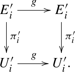
Let $\mathcal {X}=(X,\mathcal {U})$ be a complex orbifold. An orbifold vector bundle or orbibundle of rank k over $\mathcal {X}$ is a collection of vector bundles $\pi '_i :E'_{i} \rightarrow U_i'$ with fiber ${{\mathbb {C}}}^k$ for each orbifold chart $(U_i',G_i,\varphi _i,U_i)$ of $\mathcal {X}$, together with an action of $G_i$ on $E'_{i}$ by (ordinary) vector bundle maps, such that:

• 1. Each $\pi '_i$ is $G_i$-invariant, so that the following diagram is commutative for any $g \in G_i$:

  

• 2. For any injection $\lambda _{ji}:U_i' \rightarrow U_j'$ of charts on $\mathcal {X}$, there is a bundle isomorphism $\lambda _{ji}':E_i' \rightarrow \left. E_j'\right| _{\mathrm{im}(\lambda _{ji})}$, such that $\lambda _{ji}' \circ g = \lambda _{ji}(g) \circ \lambda _{ji}'$, where by $\lambda _{ji}: G_i \rightarrow G_j$ we denote the injective group homomorphism from Lemma 1 as well.

• 3. For two injections $\lambda _{ji}:U_i' \rightarrow U_j'$ and $\lambda _{kj}:U_j' \rightarrow U_k'$, we have $(\lambda _{kj} \circ \lambda _{ji})'= \lambda _{kj}' \circ \lambda _{ji}'$.

Remark 4

The total space E of an orbibundle is obtained from the local bundles $E'_i$ in the following way [21, Sec. 2.2]. Choosing small enough orbifold charts on $\mathcal {X}$, we can assume that $E_i' \cong U_i' \times {{\mathbb {C}}}^k$ and the action of $G_i$ on $U_i' \times {{\mathbb {C}}}^k$ is diagonal and acting as a subgroup of $\mathrm{GL}(k)$ on the second factor. Then since $\pi _i'$ is equivariant, setting $E_i:=E_i'/G_i$, we have a unique ’projection’ $\pi _i$, so that the following diagram commutes:

Now we can glue the sets $E_i$ in the following way, stemming from the gluing condition on $\mathcal {X}$: let $x \in U_i \cap U_j \ne \emptyset$. Then according to Definition 1 there is a chart $x \in U_k$ with injections $\lambda _{ik}:U'_k \rightarrow U_i'$ and $\lambda _{jk}:U'_k \rightarrow U_j'$, which by Definition 6 (2) induce bundle isomorphisms $\lambda _{jk}':E_k' \rightarrow \left. E_j'\right| _{\mathrm{im}(\lambda _{jk})}$ and $\lambda _{ik}':E_k' \rightarrow \left. E_i'\right| _{\mathrm{im}(\lambda _{ik})}$. Gluing $E_i$ and $E_j$ acccording to this data results in an orbifold $\mathcal {E}$ with underlying space E and an orbimap $\pi :\mathcal {E} \rightarrow \mathcal {X}$, which is locally given by the equivariant projections $\pi _i' :E_i' \rightarrow U_i'$ [21, Sec. 2.2].

Example 2

Probably the easiest but still important example of an orbibundle is the trivial line bundle, given by trivial line bundles $E_i':=U_i' \times {{\mathbb {C}}}$ on each chart $U_i'$ together with a trivial action of $G_i$ on the second factor. Then clearly $E_i \cong U_i \times {{\mathbb {C}}}$ and the total space $\mathcal {E}$ is just $\mathcal {X} \times {{\mathbb {C}}}$.

Example 3

Another very important example is that of the tangent orbibundle $T\mathcal {X}$. It can be constructed in the following natural way [9, Ex. 4.2.10]. On a chart $U_i'$, take the tangent bundle $TU_i'\cong U_i' \times {{\mathbb {C}}}^n$ and for any injection $\lambda _{ji}:U_i' \rightarrow U_j'$ of charts on $\mathcal {X}$, the bundle isomorphism $\lambda _{ji}':E_i' \rightarrow \left. E_j'\right| _{\mathrm{im}(\lambda _{ji})}$ is given by $\lambda _{ji}$ on the first factor and the Jacobian $\mathrm{Jac}(\lambda _{ji})$ on the second one. This construction obviously generalizes to the cotangent orbibundle $T^*\mathcal {X}$, (symmetric, antisymmetric) tensor orbibundles et cetera [5].

Remark 5

Locally around $x \in X$, the fiber $\pi ^{-1}(x) \subseteq T\mathcal {X}$ is not isomorphic to ${{\mathbb {C}}}^n$, but is holomorphic to a small neighbourhood of $x \in X$, because in a local chart, the actions of $g \in G_i$ on $U_i'$ and of $\mathrm{Jac}(g)$ on $T_{\phi ^{-1}(x)}U_i'$ are essentially the same.

On the other hand, even if $(X,\varDelta )$ is a smooth geometric orbifold with canonical orbifold structure $\mathcal {X}$, the underlying space of $T\mathcal {X}$ does not coincide with the ordinary tangent bundle TX, as the following example shows.

Example 4

Consider the smooth orbifold $\mathcal {X}=({{\mathbb {C}}},\mathcal {U})$ with the atlas $\mathcal {U}=\{({{\mathbb {C}}},{{\mathbb {Z}}}/2{{\mathbb {Z}}},\{x \mapsto x^2\},{{\mathbb {C}}})\}$ consisting of a single chart. The action of ${{\mathbb {Z}}}/2{{\mathbb {Z}}}$ on $U'={\mathbb {C}}$ is given by $x \mapsto -x$ and induces the diagonal action on $TU' \cong U' \times {\mathbb {C}}$ given by $(x,y) \mapsto (-x,-y)$. The quotient of $TU'$ by this action is given by

$$\begin{aligned} \tau :TU'&\rightarrow T\mathcal {X} \cong V(uv-w^2) \subseteq {\mathbb {C}}^3 \\ (x,y)&\mapsto (x^2, y^2, xy), \end{aligned}$$

which is the $A_1$-singularity. The bundle morphism $T\mathcal {X} \rightarrow \mathcal {X}$ is given by projection to the first coordinate. We see that the fibers are isomorphic to ${\mathbb {C}}$, but $T\mathcal {X} \rightarrow \mathcal {X}$ is not locally trivial around the origin.

Now having defined orbibundles, we have to ask ourselves what is a reasonable definition of (holomorphic) sections of these. Obviously for an orbibundle $\pi : \mathcal {E} \rightarrow \mathcal {X}$, a section of $\mathcal {E}$ should be a holomorphic orbimap $s:\mathcal {X} \rightarrow \mathcal {E}$ satisfying $\pi \circ s = \mathrm{id}_X$. But what does this mean on a local chart $\pi '_i:E'_i \rightarrow U'_i$? As we have an action of $G_i$ on $U_i'$ and $E_i'$, s locally corresponds to an equivariant holomorphic section $s_i:U_i' \rightarrow E_i'$, meaning $g \circ s_i = s_i \circ g$ for any $g \in G_i$. Of course the local sections must be compatible with injections as well, so that we arrive at the following definition [9, Def. 4.2.9].

Definition 7

Let $\pi : \mathcal {E} \rightarrow \mathcal {X}$ be an orbibundle. Then a holomorphic section of $\mathcal {E}$ is given by any of the two equivalent definitions:

• 1. $s:\mathcal {X} \rightarrow \mathcal {E}$ is a holomorphic orbimap satisfying $\pi \circ s = \mathrm{id}_\mathcal {X}$.

• 2. A collection of holomorphic sections $s_i:U_i' \rightarrow E_i'$ of the local bundles over charts of $\mathcal {X}$, such that for any injection $\lambda _{ji}:U_i' \rightarrow U_j'$, the following diagram commutes:

  

Remark 6

Equivariance of the local sections $s_i$ obviously is the right requirement, otherwise they would not glue to a global section $s:\mathcal {X} \rightarrow \mathcal {E}$. When (locally) the action of $G_i$ on the fiber is trivial, then of course equivariance means nothing else than invariance, as it is the case for the trivial line bundle from Example 2. Sections of this bundle clearly are in a one-to-one-correspondence with holomorphic orbimaps from $\mathcal {X}$ to ${{\mathbb {C}}}$ endowed with the trivial orbifold structure. So they are a good candidate for a structure orbisheaf on $\mathcal {X}$, see Sect. 4.

Example 5

As in Example 4, we consider the smooth orbifold with the single chart $({{\mathbb {C}}},{{\mathbb {Z}}}/2{{\mathbb {Z}}},\{x \mapsto x^2\},{{\mathbb {C}}})$. A section $s :U' \rightarrow TU'$ is equivariant if and only if $s(-x)=-s(x)$ holds for all $x \in U'$.

The other way round works quite as well. If the underlying space X of a complex orbifold is a manifold, then line bundles and Weil divisors coincide and we can pull them back to the local uniformizations, so they give orbibundles on $\mathcal {X}$. Now for example, we can ask ourselves which divisor on X gives the canonical orbibundle $K_{\mathcal {X}}$.

Example 6

To answer this question, we just have to pull back a top differential form in a local uniformization

$$\begin{aligned} \varphi :{{\mathbb {C}}}^n&\rightarrow {{\mathbb {C}}}^n \\ (x_1,\ldots ,x_n)&\mapsto (x_1^{m_i},\ldots ,x_k^{m_k},x_{k+1},\ldots ,x_n). \end{aligned}$$

We clearly have

$$\begin{aligned} \varphi ^* (\mathrm{d}z_1 \wedge \cdots \wedge \mathrm{d}z_n) = \prod _{i=1}^k m_i x_i^{m_i-1} \mathrm{d}x_1 \wedge \cdots \wedge \mathrm{d}x_n. \end{aligned}$$

Thus we have to multiply with functions that along a ramification divisor $x_i=0$ are allowed to have poles of order at most $m_i-1$. On X, this means we have to multiply with functions that on the branch divisors $z_i=0$ have poles of order at most $\frac{m_i-1}{m_i}$. So $K_\mathcal {X}$ locally is the pullback of the ${{\mathbb {Q}}}$-divisor $K_X + \varDelta$ [9, Prop. 4.4.15].

5 Orbisheaves

We first introduce the notion of an orbisheaf following [47] and [9, Def. 4.2.1].

Definition 8

Let $\mathcal {X}=(X,\mathcal {U})$ be a complex orbifold. An orbisheaf ${\mathcal {F}}$ on $\mathcal {X}$ consists of a sheaf $\mathcal {F}_i'$ over $U_i'$ for each orbifold chart $(U_i',G_i,\varphi _i,U_i)$ of $\mathcal {X}$, such that for each injection $\lambda _{ji}:U_i' \rightarrow U_j'$ there is an isomorphism of sheaves $\mathcal {F}(\lambda _{ij}):\mathcal {F}_i' \rightarrow \lambda _{ji}^* \mathcal {F}_j'$, which is functorial.

We are mainly interested in sheaves of modules over a reasonable structure sheaf, so first, we have to define such structure sheaf, see [9, Def. 4.2.2].

Definition 9

The structure orbisheaf $\mathcal {O}_{\mathcal {X}}$ is the orbisheaf consisting of structure sheaves $\mathcal {O}_{U_i'}$ on each orbifold chart $U_i'$. On a complex orbifold $\mathcal {X}$, by $\mathcal {O}_{\mathcal {X}}$ we will always denote the structure sheaf of holomorphic functions.

It is clear that this definition neither will give us a sheaf on the underlying space X nor it coincides with the holomorphic sections in the sense of Definition 7 of the trivial orbibundle, see Remark 4. We have to use local $G_i$-invariant sections of such sheaves and glue them together over X [9, Lemma 4.2.4]. We will often work with these invariant sections of orbisheaves. We will always denote sheaves on X coming from invariant local sections of orbisheaves ${\mathcal {F}}$ by $\mathcal {F}_X$. In particular $\left( \mathcal {O}_\mathcal {X}\right) _X \cong \mathcal {O}_X$ holds for the structure sheaves. We note here that the local group actions on the charts of an orbibundle induce group actions on the sheaf of local sections in such way, that the equivariant sections of the bundle are in one-to-one correspondence with the invariant sections of the sheaf. This is illustrated by the following continuation of Examples 4, 5:

Example 7

We consider the smooth complex orbifold with one single chart of the form $({{\mathbb {C}}},{{\mathbb {Z}}}/2{{\mathbb {Z}}},\{x \mapsto x^2\},{{\mathbb {C}}})$. In Example 5, we have seen that a section $s :U' \rightarrow TU'$ is equivariant if and only if $s(-x)=-s(x)$ holds. This induces an action of ${{\mathbb {Z}}}/2{{\mathbb {Z}}}$ on $\varGamma (U',TU')$ by setting $(-1).s:=-s(-x)$.

We recall that the functor $V \rightarrow V^G$ taking a vector space with an action of a finite group G to its G-invariant subspace is exact. This means in particular that for a coherent orbisheaf $\mathcal {F}$ of $\mathcal {O}_\mathcal {X}$-modules, the sheaf $\mathcal {F}_X$ made up of (locally) $G_i$-invariant sections is a coherent sheaf of $\mathcal {O}_X$-modules.

Example 8

In the case of Example 7, this means that the space of sections $s' :\mathcal {X} \rightarrow T\mathcal {X} \cong V(uv-w^2)$ is isomorphic to ${\mathcal {O}}_X$, though $T\mathcal {X} \rightarrow \mathcal {X}$ is not a line bundle in the classical sense.

As exact sequences are preserved, it also makes sense to formulate orbisheaf cohomology, orbifold Dolbeault cohomology et cetera, see Sect. 7.

6 Orbimetrics

In this section, we consider metrics on orbifolds, or orbimetrics. By the preceding considerations, it is clear that these should be invariant metrics on the local uniformizations $U_i'$ of an orbifold $\mathcal {X}=(X,\mathcal {U})$.

Definition 10

Let $\mathcal {X}=(X,\mathcal {U})$ be a complex orbifold and $\mathcal {E} \rightarrow \mathcal {X}$ an orbibundle. A Hermitian orbimetric on $\mathcal {E}$ is a collection of Hermitian metrics $h_i'$ on the local uniformizations $E_i' \rightarrow U_i'$, such that all $h_i'$ are $G_i$-invariant and all injections are Hermitian isometries.

We define a Riemannian (Hermitian) orbimetric as a collection of $G_i$-invariant Riemannian (Hermitian) metrics on the tangent spaces $TU_i' \rightarrow U_i'$ of the orbifold charts $(U_i',G_i,U_i)$, see [9, Def. 4.2.11]. Then a Kähler orbiform is a collection of $G_i$-invariant $\mathrm{d}$-closed (1, 1)-forms $\omega _i$ on the charts $U_i'$, such that the $\omega _i(*,J*)$ are Riemannian metrics on $U_i'$ [46, Def. 5.4.7].

Analogously, we can define positive line orbibundles [46, Prop. 5.4.8], Hodge orbifolds et cetera—all as $G_i$-invariant objects on the local uniformizations $U_i'$ by the usual definitions.

On the other hand, if the underlying space X of a complex orbifold $\mathcal {X}=(X,\mathcal {U})$ is smooth, then (usual) divisors or line bundles on X can be pulled back to the local uniformizations and thus define orbibundles as we have seen in Example 6 in the case of the canonical divisor.

Now when the underlying space X is a compact Kähler manifold $(X,\omega )$ with Kähler form $\omega$ (in the usual sense), then Claudon [20, Prop. 2.1] has constructed a Kähler orbiform $\omega '$ out of $\omega$. The following local example taken from [20, Rem. 2.1] illustrates how the introduction of singularities leads to nondegenerate forms in the orbifold charts.

Example 9

Let $\mathcal {X}=({{\mathbb {C}}}^n,\varDelta =\sum _{j=1}^n (1-1/m_j)\{z_j=0\})$, where $z_1,\ldots ,z_n$ are coordinates on ${{\mathbb {C}}}^n$. The uniformization $\varphi :{{\mathbb {C}}}^n \rightarrow {{\mathbb {C}}}^n$ is given by $z_j=x_j^{m_j}$. Consider the Kähler form $\omega$ given by

$$\begin{aligned} \sum _{j=1}^n i \partial {\overline{\partial }}\left| z_j \right| ^{2} = i \sum _{j=1}^n \mathrm{d}z_j \wedge \mathrm{d}{\overline{z}}_j. \end{aligned}$$

Analogous to Example 6, the pullback under $\varphi$ is

$$\begin{aligned} \varphi ^*(\omega ) = i \sum _{j=1}^n m_j^2\left| x_j\right| ^{2(m_j-1)} \mathrm{d}x_j \wedge \mathrm{d}{\overline{x}}_j, \end{aligned}$$

where $m_j=1$ if $x_j=0$ is not the restriction of a divisor $\varDelta _j$. This form is clearly degenerate. Now consider the (1, 1)-form $\omega _\varDelta$ given by

$$\begin{aligned} \omega _\varDelta = \sum _{j=1}^n i \partial {\overline{\partial }}\left| z_j \right| ^{2/m_j}. \end{aligned}$$

The pullback by $\varphi$ is

$$\begin{aligned} \varphi ^*(\omega _\varDelta ) = \sum _{j=1}^n \mathrm{d}x_j \wedge \mathrm{d}{\overline{x}}_j. \end{aligned}$$

We combine these two to a form $\omega '=\omega +\omega _\varDelta$. Then on the one hand, $\omega '$ is smooth on $X {\setminus } \mathrm{supp}(\varDelta )$, and for $c \in {{\mathbb {R}}}_{>0}$ small enough, $\omega ' \ge c\omega$ as currents. On the other hand, the pullback

$$\begin{aligned} \varphi ^*(\omega ') = i \sum _{j=1}^n (1+m_j^2\left| x_j\right| ^{2(m_j-1)}) \mathrm{d}x_j \wedge \mathrm{d}{\overline{x}}_j \end{aligned}$$

is a true Kähler form in the uniformization.

What we need here is a stronger result. Consider the following situation: $\mathcal {X}=(X,\varDelta )$ is a complex orbifold with X a manifold. Let L be an ample line bundle on the manifold X. Then according to [9, Thm. 4.3.14] and the preceding paragraph therein, the first orbifold Chern class of L is just the usual first Chern class with respect to X. Thus L (or the pullback to local uniformizations) defines an ample (or positive) line orbibundle.

Now given a Hermitian positive line bundle (L, h) on X with curvature form $\varTheta (L,h)$, such that $\omega = i\varTheta (L,h)$ is a Kähler form, we want to explicitly construct an orbimetric H on L as an orbibundle, such that $i\varTheta (L,H)$ is a Kähler orbiform.

This directly leads to the notion of singular Hermitian metrics, introduced in [25, Def. 2.1].

Definition 11

Let X be a complex manifold and (L, h) a hermitian line bundle on X. A singular Hermitian metric H is a metric on L, given in a local trivialization $L \supseteq V \cong U \times {{\mathbb {C}}}$ by $H=e^{-\phi }h$, where $\phi \in L^1_{\mathrm{loc}}(U,{{\mathbb {R}}})$ is a locally integrable function on U. We call (L, H) a singular Hermitian line bundle. Due to [46, Def. 2.3.2], the curvature current of (L, H) is given by

$$\begin{aligned} \varTheta (L,H)=\varTheta (L,h)+ \partial {\overline{\partial }}\phi . \end{aligned}$$

Thus we have the following.

Proposition 1

Let $\mathcal {X}=(X,\varDelta =\sum _{j=1}^m (1-1/m_j)\varDelta _j)$ be a smooth compact complex orbifold. For any $j=1,\ldots ,m$, let $s_j \in \mathcal {O}_X(\varDelta _j)$ be a section defining $\varDelta _j$. Let (L, h) be a positive Hermitian line bundle on X.

Let $C \in {\mathbb {R}}_{>0}$ and set $H=e^{-\phi }h$ for

$$\begin{aligned} \phi = C \sum _{j=1}^{m} \left| s_j\right| ^{2/m_j}, \end{aligned}$$

where $\left| s_j\right|$ is with respect to some smooth metric on $\mathcal {O}_X(\varDelta _j)$.

Then for C small enough, (L, H) is a positive line orbibundle. In particular, the form $\omega '$ given by

$$\begin{aligned} \omega ':= i \varTheta (L,H)= i \varTheta (L,h) + i\partial {\overline{\partial }}\phi \end{aligned}$$

is a Kähler orbiform.

Proof

Since (L, h) is positive, the form $\omega =i \varTheta (L,h)$ is a Kähler form on the complex manifold X. On the other hand, locally in a chart, we can choose a constant $C'$, such that

$$\begin{aligned} \omega + i\partial {\overline{\partial }}C' \sum _{j=1}^{m} \left| s_j\right| ^{2/m_j} \end{aligned}$$

is positive. Since $\mathcal {X}$ is compact, we can thus choose a global constant C with the required properties. The computations are performed in the proof of Proposition 2.1 in the arXiv-version of [20]. $\square$

We finally note that we can integrate n-forms by a partition of unity and by setting

$$\begin{aligned} \int _{U_i} \sigma := \frac{1}{G_i} \int _{U_i'} \varphi ^*(\sigma ) \end{aligned}$$

in a local uniformization $(U_i',G_i,\varphi _i,U_i)$, see e.g. [9, Eq. (4.2.2)]. Thus if $(\mathcal {E},h)$ is a Hermitian orbibundle on a complete Kähler orbifold $(\mathcal {X},\omega ')$, we have a scalar product

$$\begin{aligned} \left\langle s_1, s_2 \right\rangle := \int _X \left\langle s_1, s_2 \right\rangle _{h} \mathrm{d}V_\omega \end{aligned}$$

for sections of $\mathcal {L}$ and an associated $L^2$-norm $\left| \cdot \right| _h$, see [46, Sec. 5.4.2].

By the above considerations, it becomes clear what a singular Hermitian orbibundle should be.

Definition 12

Let $\mathcal {X}$ be a complex orbifold and $(\mathcal {E},h)$ a Hermitian orbibundle on X. A singular Hermitian metric H on $\mathcal {E}$ is a metric on $\mathcal {E}$, given in an orbifold chart $(U',G,U)$ by $H=e^{-\phi }h$, where $\phi \in L^1_{\mathrm{loc}}(U',{{\mathbb {R}}})$ is a locally integrable G-invariant function on $U'$. We call $(\mathcal {E},H)$ a singular Hermitian orbibundle. The curvature current of $(\mathcal {E},H)$ is locally given by

$$\begin{aligned} \varTheta (\mathcal {E},H)=\varTheta (\mathcal {E},h)+ \partial {\overline{\partial }}\phi . \end{aligned}$$

7 The orbifold universal cover and the $\varGamma$-reduction

Definition 13

The orbifold fundamental group of a geometric orbifold $\mathcal {X}=(X,\varDelta )$ is the quotient

$$\begin{aligned} \pi _1(X,\varDelta ):=\pi _1(X {\setminus } \mathrm{supp}(\varDelta )) / \langle \gamma _i^{m_i}, i \in I \rangle , \end{aligned}$$

where for each $i \in I$, $\gamma _i$ is a small loop around a general point of the divisor $\varDelta _i$, and $\langle \gamma _i^{m_i}, i \in I \rangle$ is the normal subgroup generated by the $\gamma _i^{m_i}$.

Associated to the orbifold fundamental group, there is the notion of orbifold universal cover $\pi :\widetilde{\mathcal {X}} \rightarrow \mathcal {X}$. It is a ramified Galois cover between complex analytic spaces, étale over $X {\setminus } \mathrm{supp}(\varDelta )$.

Remark 7

Let $\mathcal {X}=(X,\varDelta )$ be a smooth geometric orbifold. Then over a (sufficiently small) orbifold chart $(U_i',G_i,\varphi _i,U_i)$ of X as in Remark 2, the preimage under the orbifold universal cover $\pi :\widetilde{\mathcal {X}} \rightarrow \mathcal {X}$ has connected components $V_i$, such that $V_i$ has a local uniformization $(V_i',H_i,\psi _i,V_i)$ with $H_i$ a subgroup of $G_i$. In particular, since $G_i$ is abelian, $H_i$ is so as well and $V_i$ only has toric singularities. Locally, $\left. \pi \right| _{V_i} :V_i \rightarrow U_i$ is a quotient by $G_i / H_i$ and the lift $V_i' \rightarrow U_i'$ is just the identity [20, Rem. 1.2]. In particular, we have the following commutative diagram:

So in a sense, the universal cover is locally trivial as we expect from a cover. In particular, we see that for an orbimetric $\omega$ on ${\mathcal {X}}$ and the pullback $\pi ^* (\omega )$, the pullbacks to the local uniformizations are identical.

As we mentioned before, the analogy between geometric and classical orbifolds not only holds if the underlying space is smooth. In particular, on the underlying space X of a classical complex orbifold $\mathcal {X}=(X,\mathcal {U})$ one always can define a divisor $\varDelta$, such that the geometric orbifold $(X,\varDelta )$ has the canonical orbifold structure $\mathcal {X}=(X,\mathcal {U})$, see [10, p. 561]. In particular, this holds for the orbifold universal cover $\widetilde{\mathcal {X}}$. But we do not need the structure of a geometric orbifold on $\widetilde{\mathcal {X}}$ here.

An important observation for us will be that if X is a complex analytic space, $\varDelta _1,\ldots ,\varDelta _m$ are smooth prime divisors on X with normal crossings, and small loops $\gamma _i$ around general points of $\varDelta _i$ are of finite order $m_i$ in $\pi _1(X {\setminus }(\varDelta _1 \cup \cdots \cup \varDelta _m))$, then

$$\begin{aligned} \pi _1(X {\setminus }(\varDelta _1 \cup \cdots \cup \varDelta _m)) = \pi _1\left( X,\sum _{i=1}^m \left( 1-\frac{1}{m_i}\right) \varDelta _i\right) . \end{aligned}$$

Note that by the Hopf–Rinow-Theorem for orbifolds [16, Thm. 4.2.2], the orbifold covers of a complete orbifold (with respect to an orbimetric $\omega '$, cf. Section 5), are complete with respect to the pullback metric (since orbifold geodesics can be lifted). In particular, the orbifold universal cover of a compact orbifold with a Hermitian orbimetric is complete with respect to the pullback orbimetric.

An important ingredient for us is the $\varGamma$-reduction or Shafarevich map. This construction has been introduced by Kollár for proper normal projective varieties [42, Def. 1.4] and independently by Campana for compact Kähler manifolds [14, Thm. 3.5,Def. 3.8]. Formulated on the universal cover ${\widetilde{X}}$ of a compact Kähler manifold X, it says that there is a unique almost holomorphic fibration ${\widetilde{\gamma }} :{\widetilde{X}} \dasharrow \varGamma ({\widetilde{X}})$, such that any compact irreducible subvariety of ${\widetilde{X}}$ through a very general point $x \in {\widetilde{X}}$ is contained in the fiber ${\widetilde{\gamma }}^{-1}({\widetilde{\gamma }}(x))$. The general fibers of ${\widetilde{\gamma }}$ are exactly the maximal compact subvarieties of ${\widetilde{X}}$. The action of $\pi _1(X)$ on ${\widetilde{X}}$ descends to $\varGamma ({\widetilde{X}})$ and thus by quotienting induces an almost holomorphic fibration $\gamma :X \dasharrow \varGamma (X)$, of which the fibers are the maximal subvarieties with finite fundamental group. In turn, the connected components of the preimages of such fibers are exactly the fibers of ${\widetilde{\gamma }}$.

This concept has been generalized by Claudon in [20] to smooth geometric orbifolds—using Kähler orbiforms as in Example 9—, see also [12, Sec. 12.5]. We have the following [20, Thm. 0.2].

Theorem 1

Let $\mathcal {X}=(X,\varDelta )$ be a compact smooth geometric Kähler orbifold and $\pi :\widetilde{\mathcal {X}} \rightarrow \mathcal {X}$ its orbifold universal cover. There are almost holomorphic fibrations ${\widetilde{\gamma }} :\widetilde{\mathcal {X}} \dasharrow \varGamma (\widetilde{\mathcal {X}})$ and $\gamma :\mathcal {X} \dasharrow \varGamma (\mathcal {X})$ , such that the diagram

commutes and the following hold:

• 1. If $V \subseteq X$ is a smooth subvariety meeting $\varDelta$ transversally, such that the image of $\pi _1(V,\left. \varDelta \right| _V)$ in $\pi _1(X,\varDelta )$ is finite, and V meets the fiber of $\gamma$ through a very general point, then V is contained in this fiber.

• 2. Every compact irreducible subvariety of $\widetilde{\mathcal {X}}$ through a very general point $x \in \widetilde{\mathcal {X}}$ is contained in the fiber ${\widetilde{\gamma }}^{-1}({\widetilde{\gamma }}(x))$.

• 3. There exist open subsets $X^0 \subset X$ and $\varGamma (\mathcal {X})^0 \subset \varGamma (\mathcal {X})$, such that $\left. \gamma \right| _{X^0} :X^0 \rightarrow \varGamma (\mathcal {X})^0$ is a proper holomorphic, topologically locally trivial fibration.

Remark 8

Theorem 0.2 of [20] is formulated only on the universal cover, while [12, Thm. 12.23] is formulated on the orbifold $\mathcal {X}$ itself. The connection between the both is [20, Le. 2.2]. The third item has not been formulated in the orbifold case, but the argument at the end of the proof of Proposition 2.4 in [42] works here as well.

We also note that [20] uses a regularization $\varDelta _{\mathrm{reg}}:= \sum (1-1/d_i) \varDelta _i$ of the orbifold divisor $\varDelta = \sum (1-1/m_i) \varDelta _i$, where $d_i | m_i$ is the order of $\gamma _i$ in $\pi _1(X,\varDelta )$. The passage from $(X,\varDelta )$ to $(X,\varDelta _{\mathrm{reg}})$ does not change the orbifold fundamental group, but it changes the orbofild charts and thus also the orbimetrics involved. The only reason for replacing $\varDelta$ by $\varDelta _{\mathrm{reg}}$ is that on $\widetilde{{\mathcal {X}}}$, the orbifold charts are given by the structure of the underlying complex analytic space and in particular, do not ramify in codimension 1. But the proof of [20, Thm. 0.2] works as well if the charts on $\widetilde{{\mathcal {X}}}$ do ramify in codimension 1, so the only thing we have to make sure is that we use the right orbifold structure on $\widetilde{{\mathcal {X}}}$, so that $\widetilde{\mathcal {X}} \rightarrow \mathcal {X}$ is a locally trivial orbifold cover.

8 Dolbeault and $L^2$-cohomology for Kähler orbifolds

Following [5, Sec. 5], we can define orbifold Dolbeault cohomology for complete Kähler orbifolds $(\mathcal {X}=(X,\mathcal {U}),\omega )$ in the following way. Denote by $\varOmega _X^{p,q}$ the sheaf of (p, q)-orbiforms, defined by the G-invariant (p, q)-forms on the orbifold charts. Since these sections are G-invariant on each chart, the define a sheaf on X, which by abuse of notation we denote by $\varOmega ^{p,q}_X$ as well. The exterior derivative and the Dolbeault operators $\mathrm{d}= \partial + {\overline{\partial }}$ are G-equivariant and thus well defined, with

$$\begin{aligned} \partial :\varOmega ^{p,q}_X \rightarrow \varOmega ^{p+1,q}_X, \qquad {\overline{\partial }}:\varOmega ^{p,q}_X \rightarrow \varOmega ^{p,q+1}_X. \end{aligned}$$

Definition 14

The (p, q)-th orbifold Dolbeault cohomology group is defined by

$$\begin{aligned} H^{p,q}(X) := \frac{\ker ({\overline{\partial }}:\varOmega _X^{p,q}(X) \rightarrow \varOmega _X^{p,q+1}(X))}{\mathrm{im}({\overline{\partial }}:\varOmega _X^{p,q-1}(X) \rightarrow \varOmega _X^{p,q}(X))}. \end{aligned}$$

If $\mathcal {E} \rightarrow \mathcal {X}$ is a holomorphic orbibundle, then one can similarly define the Dolbeault complex $(\varOmega _X^{p,q}(X,\mathcal {E}),{\overline{\partial }}^\mathcal {E})$ of (p, q)-orbiforms with values in $\mathcal {E}$ as well as Dolbeault cohomology groups $H^{p,q}(X,\mathcal {E})$. Then the Dolbeault isomorphism for orbifolds holds, see [46, Sec. 5.4.2]. Now let $\mathcal {E}$ be endowed with a (smooth or singular) Hermitian orbimetric h. Following [46, Eq. (B.4.12)], we define the $L^2$-spaces

$$\begin{aligned} L^2_{p,q}(X,\mathcal {E}):=\left\{ s \in \varOmega _X^{p,q}(X,\mathcal {E});~ \int _X \left| s\right| ^2_h dV_\omega < \infty \right\} , \end{aligned}$$

and the $L^2$-Dolbeault cohomology groups by

$$\begin{aligned} H_{(2)}^{p,q}(X,\mathcal {E}) := \frac{\ker ({\overline{\partial }}^\mathcal {E}) \cap L^2_{p,q}(X,\mathcal {E})}{\mathrm{im}({\overline{\partial }}^\mathcal {E}) \cap L^2_{p,q}(X,\mathcal {E}) }. \end{aligned}$$

Well-definedness follows from [4, Sec. C.3], which can be directly transferred to complete Kähler orbifolds.

9 $L^2$-vanishing for orbifolds

The singular Hermitian metrics from Sect. 5 will be more useful to us than just for constructing Kähler orbiforms from positive line bundles on the underlying space. For a singular Hermitian line bundle (L, H) with $H=e^{-\phi }h$ on a complex manifold X, there is the notion of the $L^2$-sheaf $\mathcal {L}^2(L,H)$ of locally square-integrable functions with respect to H, given by

$$\begin{aligned} \mathcal {L}^2(L,H)(U) = \{ \sigma \in \varGamma (U,L);~ \left| \sigma \right| _h^2 e^{-\phi } \in L_{\mathrm{loc}}^1(U)\}, \end{aligned}$$

see [54, Eq. (3.1)]. In particular, the function $\phi$ defines a singular Hermitian metric $e^{-\phi } z {\overline{z}}$ on the trivial line bundle $X \times {{\mathbb {C}}}$. This leads us to the definition of the multiplier ideal sheaf $\mathcal {I}(\phi ):=\mathcal {L}^2(X \times {{\mathbb {C}}},e^{-\phi })$. In particular, $\mathcal {L}^2(L,H) = L \otimes \mathcal {I}(\phi )$. Note that the functions $\phi$ may only be given locally, so in this notation $\phi$ can rather be seen as a collection of locally defined functions. On the other hand, it may still be possible to express $\phi$ globally by certain sections as e.g. in Proposition 1.

A plurisubharmonic or shortly psh function is defined by certain semicontinuity properties, see e.g. [23, Def. (1.4)]. We will use the following characterization from [46, Prop. B.2.10, B.2.16], which is much more immediate in our setting.

Definition 15

Let X be a complex analytic manifold. A function $\phi : X \rightarrow {{\mathbb {R}}}$ is called plurisubharmonic or psh, if $i\partial {\overline{\partial }}\phi$ is a semipositive form. It is called strictly psh, if $\phi \in L^1_\mathrm{loc}(X)$ and $i\partial {\overline{\partial }}\phi$ is (strictly) positive.

The point is that obviously on the one hand, a singular Hermitian metric H on a positive Hermitian line bundle (L, h) defined by a psh function $\phi$ gives a positive (1, 1)-form $\omega =i\varTheta (L,H)$.

On the other hand, we have the Nadel coherence theorem [23, Prop. (5.7)], stating that $\mathcal {I}(\phi )$ is a coherent sheaf if $\phi$ is psh. This can be easily transformed to the orbifold setting. First let us define the analogue of the multiplier ideal sheaf following [9, Def. 5.2.9].

Definition 16

Let $\mathcal {X}$ be a complex orbifold and let $(\mathcal {E},H=he^{-\phi })$ be a singular Hermitian orbibundle on $\mathcal {X}$. The multiplier ideal orbisheaf $\mathcal {I}_\mathcal {X}(\phi )$ is the orbisheaf defined on local orbifold charts $(U', G, U)$ by

$$\begin{aligned} \mathcal {I}_\mathcal {X}(\phi )(U')=\left\{ f \in \mathcal {O}_{\mathcal {X}}^{G}(U_i');~ |f|^2e^{-\phi } \in L^1_{\mathrm{loc}}(U')\right\} . \end{aligned}$$

The orbifold version of Nadel’s coherence theorem follows from the standard version since the functor taking G-invariant sections is exact by finiteness of G. Thus we have:

Theorem 2

(Nadel’s coherence theorem for orbifolds) Let $\mathcal {X}$ be a complex orbifold and $(\mathcal {E},H=he^{-\phi })$ be a singular Hermitian orbibundle on $\mathcal {X}$. Then the (pushforward of the) multiplier ideal orbisheaf $\mathcal {I}_\mathcal {X}(\phi )$ is a coherent sheaf of $\mathcal {O}_X$-modules on X.

The next step to go now is the Nadel vanishing theorem. An orbifold version appeared in [26, Thm. 6.5]. The statement in the following theorem slightly differs from this version, as we explain below.

Theorem 3

(Nadel’s vanishing theorem for orbifolds) Let $(\mathcal {X},\omega )$ be a compact Kähler orbifold. Let $(\mathcal {L},H=he^{-\phi })$ be a singular Hermitian orbibundle on $\mathcal {X}$. Assume that there exists a constant $c \in {{\mathbb {R}}}_{>0}$, such that $i\varTheta (\mathcal {L},H)\ge c\omega$. Then

$$\begin{aligned} H^q(X,K_\mathcal {X} \otimes \mathcal {L} \otimes \mathcal {I}_\mathcal {X}(\phi ))=0 ~\quad \mathrm {for}~ q \ge 1. \end{aligned}$$

The authors of [26, Thm. 6.5] use $L^2$-estimates on the smooth locus of X. In contrary, we use $L^2$-estimates for locally invariant forms in the orbifold charts, see Proposition 2 below. This means that in Thm. 3, we can allow a ramification divisor $\varDelta$ (i.e. we have $K_\mathcal {X}=K_X+\varDelta$), and do not have to assume invertibility of $K_\mathcal {X} \otimes \mathcal {L}$ on X.

It turns out that for us these $L^2$-estimates are more important than the statement of Theorem 3. The following proposition states the orbifold version of [24, Thm. 5.1].

Proposition 2

Let $(\mathcal {X},\omega )$ be a complete Kähler orbifold. Let $(\mathcal {E},H=he^{-\phi })$ be a singular Hermitian orbibundle on $\mathcal {X}$, where h is a smooth Hermitian orbimetric on $\mathcal {E}$. Assume that there exists a constant $c \in {{\mathbb {R}}}_{>0}$, such that $i\varTheta (\mathcal {E},H)\ge c\omega \otimes \mathrm{id}_{\mathcal {E}}$. Then for any ${\overline{\partial }}$-closed form $g \in L_{n,q}^2(\mathcal {X}, \mathcal {E})$, there is a form $f \in L_{n,q-1}^2(\mathcal {X},\mathcal {E})$, with ${\overline{\partial }}f=g$ and

$$\begin{aligned} \int _X \left| f\right| _H^2 \mathrm{d}V_{\omega } \le \frac{1}{qc} \int _X \left| g\right| _H^2 \mathrm{d}V_{\omega }. \end{aligned}$$

The rest of this section is devoted to the proof of the above proposition. We will follow the lines of the original proof in [24] for manifolds, which we adopt to the orbifold case by considering G-invariant objects on the orbifold charts $(U',G,U)$. We note that G-invariance of ${\overline{\partial }}$-solutions has been considered in [48, Prop. 1.1].

To make the notation easier and the proof a little bit shorter, in the statement of Proposition 2, we assume that $\omega$ is a complete metric. The proof works in a more general setting by approximation of $\omega$ with complete metrics, see [24, p. 474], but we omit this here, since in our setting, we can work with a complete orbimetric $\omega$ in the first place, namely the pullback metric on the universal cover of a compact Kähler orbifold.

Proof

(Proof of Proposition 2) The strategy of the proof is as follows. First, one proves the statement in the case that H is a smooth metric. Then, one shows that the singular metric H can be approximated by smooth metrics in a reasonable way. In a last step, one finally proves that the statement holds for the approximated singular metric as well.

Step 1: Case of a smooth metric H.

We follow the lines of [24, Sec. 4] here, which we have to adapt to the orbifold setting. The main difference is that we have to deal with G-invariant sections on the orbifold charts $(U',G,U)$. So we have to make sure that everything is well defined.

We denote by $\mathcal {D}_{p,q}(\mathcal {X},\mathcal {E})$ the space of smooth (p, q)-orbiforms with compact support and with values in $\mathcal {E}$. With $L_{p,q}^2(\mathcal {X},\mathcal {E})$, we denote the Hilbert-space of (p, q)-forms with values in $\mathcal {E}$ and $L_{\mathrm {loc}}^2$-coefficients, equipped with the norm

$$\begin{aligned} \Vert u \Vert ^2 := \int _X |u|_H^2 \quad \mathrm{d}V_{\omega }. \end{aligned}$$

All these forms are given by G-invariant forms on a chart $(U',G,U)$. We note that $\mathcal {D}_{p,q}(\mathcal {X},\mathcal {E})$ is dense in $L_{p,q}^2(\mathcal {X},\mathcal {E})$. In particular, ${\overline{\partial }}u \in L_{p,q+1}^2(\mathcal {X},\mathcal {E})$ for $u \in \mathcal {D}_{p,q}(\mathcal {X},\mathcal {E})$. Thus the ${\overline{\partial }}$-operator induces two operators

$$\begin{aligned} L_{p,q-1}^2 \xrightarrow {T} L_{p,q}^2 \xrightarrow {S} L_{p,q+1} \end{aligned}$$

with dense domains $\mathrm {Dom} T$, $\mathrm {Dom} S$, defined by $Tu ={\overline{\partial }}u$ as long as ${\overline{\partial }}u \in L_{p,q}^2$ (and S defined analogously). The operators T and S are unbounded but closed [38, p. 78]. We denote by $T^*$ and $S^*$ the adjoint operators of T and S respectively.

By [38, Lem. 5.2.1], $\mathcal {D}_{p,q}(\mathcal {X},\mathcal {E})$ is dense in $\mathrm {Dom} T^* \cap \mathrm {Dom} S$ for the graph norm $u \mapsto \Vert u\Vert + \Vert T^* u\Vert + \Vert S u \Vert$. Here the proof of [38, Lem. 5.2.1] can be directly transferred to the orbifold case, since it is local and in the essential [38, Lem. 5.2.2], we can choose all objects to be G-invariant, such that also the operator $J_\epsilon$ (which produces smooth forms out of $L^2$-forms) defined therein is G-invariant and we can approximate $u \in \mathrm {Dom} T^* \cap \mathrm {Dom} S$ by smooth forms $J_\epsilon u \xrightarrow [\epsilon \rightarrow 0]{} u$.

Now let ${\overline{\partial }}^*$ be the adjoint of ${\overline{\partial }}$, defined for all forms $u \in \mathcal {D}_{p,q-1}(\mathcal {X},\mathcal {E})$, $v \in \mathcal {D}_{p,q}(\mathcal {X},\mathcal {E})$ by

$$\begin{aligned} \int _X \langle {\overline{\partial }}u, v \rangle \mathrm{d}V_{\omega } = \int _X \langle u, {\overline{\partial }}^* v \rangle \mathrm{d}V_{\omega }. \end{aligned}$$

By the above considerations, the operator $T^*$ coincides with the operator ${\overline{\partial }}^*$.

We denote by $L: \mathcal {D}_{p,q}(\mathcal {X},\mathcal {E}) \rightarrow \mathcal {D}_{p+1,q+1}(\mathcal {X},\mathcal {E})$ the operator defined by $L u:= \omega \wedge u$ and by $\varLambda$ its adjoint with respect to the $L^2$-metric as above. Moreover, we have the operators ${\overline{\partial }}$ and ${\overline{\partial }}^*$ from above as well as $\partial$ and $\partial ^*$. The self-adjoint operators $\varDelta :=\partial \partial ^* + \partial \partial ^*$ and ${\overline{\varDelta }}:={\overline{\partial }}{\overline{\partial }}^* + {\overline{\partial }}{\overline{\partial }}^*$ satisfy the Bochner-Kodaira-Nakano identity ${\overline{\varDelta }}=\varDelta +[i\varTheta (\mathcal {E},H),\varLambda ]$. Obviously this identity holds in the orbifold setting, since it can be proven locally.

From this we get the Bochner-Kodaira-Nakano-inequality [24, Lem. 4.4], stating that for all forms $u \in \mathcal {D}_{n,q}(\mathcal {X},\mathcal {E})$, we have

$$\begin{aligned} \Vert {\overline{\partial }}u\Vert ^2 + \Vert {\overline{\partial }}^* u\Vert \ge \int _X \langle [i\varTheta (\mathcal {E},H),\varLambda ] u, u\rangle \mathrm{d}V_{\omega }. \end{aligned}$$

It follows easily by integrating

$$\begin{aligned}&\int _X \langle [i\varTheta (\mathcal {E},H),\varLambda ] u, u\rangle \mathrm{d}V_{\omega }\\&\quad = \int _X \langle {\overline{\varDelta }}, u\rangle \mathrm{d}V_{\omega }- \int _X \langle \varDelta u, u\rangle \mathrm{d}V_{\omega } \\&\quad = \int _X \langle {\overline{\partial }}u , {\overline{\partial }}u\rangle \mathrm{d}V_{\omega } +\int _X \langle {\overline{\partial }}^* u , {\overline{\partial }}^* u\rangle \mathrm{d}V_{\omega }\\&\qquad - \int _X \langle \partial u , \partial u\rangle \mathrm{d}V_{\omega } -\int _X \langle \partial ^* u , \partial ^* u\rangle \mathrm{d}V_{\omega }, \end{aligned}$$

which obviously holds in the orbifold setting. Thus for every form $u \in \mathrm {Dom} T^* \cap \mathrm {Dom} S$, we have the inequalities

$$\begin{aligned} \Vert T^* u\Vert ^2 + \Vert S u\Vert \ge \int _X \langle [i\varTheta (\mathcal {E},H),\varLambda ] u, u\rangle \mathrm{d}V_{\omega } \ge 0, \end{aligned}$$

where the last one follows from [24, Lem. 3.1]. Now we let $p=n=\dim (X)$. With [24, Eq. (3.1), (3.4)], we get

$$\begin{aligned} |\langle \alpha , \beta \rangle |^2 \le \frac{1}{qc} |\alpha |_{H}^2 \langle [i\varTheta (\mathcal {E},H),\varLambda ] \beta , \beta \rangle \end{aligned}$$

for all $\alpha , \beta \in \bigwedge ^{n,q} T\mathcal {X}_x \otimes \mathcal {E}_x$. Then together with the Cauchy-Schwarz inequality, the above yields

$$\begin{aligned} |( g | u ) |^2 \le \frac{1}{qc} \int _X |g|_{H}^2 \mathrm{d}V_{\omega } \cdot (\Vert S u\Vert ^2 + \Vert T^* u\Vert ^2), \end{aligned}$$

for all $u \in \mathrm {Dom} T^* \cap \mathrm {Dom} S$, where $(*|*)$ is the inner product of the Hilbert space $L^2_{n,q}$. Now we decompose orthogonally $u=u_1+u_2$, with $u_1 \in \ker S$ and $u_2 \in (\ker S)^\bot \subseteq \ker T^*$. Since $g \in \ker S$, we deduce

$$\begin{aligned} |( g | u ) |^2=|( g | u_1 ) |^2 \le \frac{1}{qc} \int _X |g|_{H}^2 \mathrm{d}V_{\omega } \cdot \Vert T^* u\Vert ^2 \end{aligned}$$

as in [24, p. 473]. Now by the Hahn-Banach theorem for Hilbert spaces applied to the linear functional $T^* u \mapsto ( u | g )$, there exists $f \in L^2_{n,q-1}$, such that $(u|g)=(T^* u|f)$ for all $u \in \mathrm {Dom} T^*$ (i.e. $g=T^*f$) and $\Vert f\Vert ^2 \le \frac{1}{qc} \int _X |g|_{H}^2 \mathrm{d}V_{\omega }$. Thus the case of a smooth metric H is proven.

Step 2: Approximation by smooth metrics.

Here we follow the lines of [24, Sec. 9]. Again we have to be careful if everything can be defined properly by invariant objects on orbifold charts.

First we note that $\mathcal {X}$ allows a smooth exhaustion function (in particular, the lifts to the orbifold charts are smooth and G-invariant functions). Then we follow [24, Sec. 8] in order to construct a family of functions $(\phi _\epsilon )_{\epsilon \in (0,1]}$ converging to $\phi$ pointwise for $\epsilon \rightarrow 0$. We note that the exponential map $\exp :TU' \rightarrow U'$ is G-equivariant in each orbifold chart $(U',G,U)$. Then with the smooth function $\chi :{\mathbb {R}} \rightarrow {\mathbb {R}}$ defined as in [24, Eq. (8.1)], we can define for any $\epsilon \in (0,1]$:

$$\begin{aligned} \phi _\epsilon (x) := \frac{1}{C\epsilon ^{2n}}\int _{\zeta \in T_x U'} \phi (\exp _x(\zeta ))\chi '(|\zeta |^2/\epsilon ^2) \mathrm{d}\lambda (\zeta ), \end{aligned}$$

where $C=\int _{\zeta \in T_x U'} \chi '(|\zeta |^2)\mathrm{d}\lambda (\zeta )$. Since $\phi$ is G-invariant and $\exp$ is G-equivariant, we get that $\phi _\epsilon$ is G-invariant as required and defined on any compact of $\mathcal {X}$ when $\epsilon$ is small enough. In particular, we can choose a smooth exhaustion function $\psi$ in such way that $\phi _\epsilon$ is smooth in a neighbourhood of each compact $K_\epsilon :=\{x \in \mathcal {X}; \psi (x) \le 1/\epsilon \}$. Moreover, we choose $\rho :{\mathbb {R}} \rightarrow {\mathbb {R}}$ smooth, such that $\rho (t)=1$ for $t \le 1/2$ and $\rho (t)=0$ for $t\ge 1$. So we get smooth functions $\phi _\epsilon (x)\rho (\epsilon \psi (x))$ defined on the whole of $\mathcal {X}$. Since [24, Lem. 8.4] is local in nature, we can follow the proof on [24, p. 504] to obtain a family $({\hat{\phi }}_\epsilon )_{\epsilon \in (0,1]}$ with

$$\begin{aligned} \lim _{\epsilon \rightarrow 0} {\hat{\phi }}_\epsilon (x) =\phi (x) \quad \mathrm {~for~all~} x \in \mathcal {X}. \end{aligned}$$

Since the function $\tau (a)$ from [24, p. 502] is G-invariant, also the functions $\lambda _\epsilon$ given by [24, Eq. (8.24)] are. Also the forms $\gamma _\epsilon$ are G-invariant, so the rest of the proof of [24, Thm. 9.1] goes through (everything here can be defined locally by a partition of unity).

The ${\hat{\phi }}_\epsilon$, $\lambda _\epsilon$, $\gamma _\epsilon$ defined this way yield a sequence of smooth Hermitian metrics $|*|_\mu :=|*|_he^{-{\hat{\phi }}_{1/\mu }}$ on $\mathcal {E}$ (where $|*|_h$ is the fixed smooth metric on $\mathcal {E}$ from the proposition), with the following properties (compare [24, Hypothèses p. 476]):

• 1. for all $\mu =1,2,\ldots$ and $e \in E$, we have $|e|_\mu \le |e|_{\mu +1}$,

• 2. the metric $|*|_\mu$ fiberwise tends to $|*|_H$ almost everywhere on $\mathcal {X}$,

• 3. $i \partial {\overline{\partial }}{\hat{\phi }}_{1/\mu } \ge \gamma _{1/\mu } - \lambda _{1/\mu }\omega$,

• 4. $\lambda _{1/\mu }$ tends to zero almost everywhere on $\mathcal {X}$,

• 5. $\gamma _{1/\mu }$ tends to $i\partial {\overline{\partial }}\phi$ almost everywhere on $\mathcal {X}$,

• 6. there is a continuous function $\lambda :=\lambda _1$ on $\mathcal {X}$, such that $0 \le \lambda _{1/\mu } \le \lambda$ for any $\mu$.

Step 3: Case of a singular metric H.

Now we deduce the statement of Proposition 2 in the general case of a singular metric $|*|_H=|*|_h e^{-\phi }$ from the smooth case (Step 1) by approximating $\phi$ with smooth metrics ${\hat{\phi }}_{1/\mu }$ as in Step 2. We follow the lines of [24, Démonstration,  p. 476]. We fix an approximation $|*|_\mu =|*|_h e^{-{\hat{\phi }}_{1/\mu }}$. For any $\mu$, we index by $\mu$ all related objects: the norm $\Vert *\Vert _\mu$ on the Hilbert space $L^2_{n,q}:=L^2_{n,q}(\mathcal {X},\mathcal {E})_\mu$, the operators $T_\mu :L_{n,q-1}^2 \rightarrow L_{n,q}^2$ and $S_\mu :L_{n,q}^2 \rightarrow L_{n,q+1}^2$.

Since $\omega$ is complete, by [24, Def. 1.3], we have an exhaustive series of compacts $(K_\nu )_{\nu \in {\mathbb {N}}}$ in X and truncating smooth functions $\chi _\nu$ with compact support, such that $0 \le \chi _\nu \le 1$, $\left. \chi _\nu \right| _{K_\nu } \equiv 1$, and $|\mathrm{d}\chi _\nu | \le 1/\nu$. We define

$$\begin{aligned} \theta _{\mu ,\nu }:=\gamma _{1/\mu } \otimes \mathrm{id}_E + i\varTheta (\mathcal {E},\Vert *\Vert _h) +\frac{1}{q\nu }\omega \otimes \mathrm{id}_\mathcal {E}. \end{aligned}$$

With these definitions, we arrive (without any difference to the manifold case, but note that in [24], there are a few typos: $\varTheta$ in [24, Eq. (5.7)] should write $\theta$ and (4.3), (4.7) in the first line of [24, p. 477] should write (5.3), (5.7)) at the inequality [24, Eq. (5.8)]:

$$\begin{aligned} |(g|u)_\mu |^2 \le A_{\mu ,\nu } \left( \Vert T^*_\mu u \Vert ^2_\mu + \Vert S_\mu u \Vert ^2_\mu + q \Vert \lambda _\mu \chi _\nu \Vert ^2_\mu + \frac{2}{\nu }\Vert u\Vert ^2_\mu \right) , \end{aligned}$$

which holds for all $\mu , \nu \in {\mathbb {N}}$ and $u \in \mathrm {Dom}T^* \cap \mathrm {Dom}S$ with $A_{\mu ,\nu }$ given by

$$\begin{aligned} A_{\mu ,\nu }:= \frac{\nu +1}{\nu } \int _{\mathrm {Supp} \chi _\nu } |g|^2_{\mu ,\theta _{\mu ,\nu }} \mathrm{d}V_\omega . \end{aligned}$$

Now the statement of the proposition is proven by induction on $n-q$, starting with the case $q=n$, where of course S vanishes. Thus for any fixed $\nu$, the Hahn-Banach theorem provides us with a sequence of operators $f_\mu , w_\mu , v_\mu \in L^2_{n,n-1}(\mathcal {X},\mathcal {E})_\mu$, satisfying

$$\begin{aligned}&\int _X |f_\mu |_\mu ^2+ |f_\mu |_\mu ^2 + |f_\mu |_\mu ^2 \mathrm{d}V_\omega \le A_{\mu ,\nu } \quad \mathrm {and} \\&\chi _\nu g = {\overline{\partial }}f_\mu + q^{1/2} \lambda _\mu ^{1/2} \chi _\nu v_\mu + \left( \frac{2}{\nu }\right) ^{1/2} w_\mu \end{aligned}$$

for all $u \in \mathrm {Dom}T^*$. We choose subseries of $(f_\mu )_\mu$ and $(w_\mu )_\mu$, that in $L^2_\mathrm{loc}$ converge weakly to limits $f^\nu$ and $w^\nu$ respectively. On the other hand, with the above considerations, $q^{1/2} \lambda _\mu ^{1/2} \chi _\nu v_\mu$ tends to zero in $L^1_\mathrm{loc}$, so

$$\begin{aligned} \chi _\nu g ={\overline{\partial }}f^\nu + \left( \frac{2}{\nu }\right) ^{1/2} w^\nu \mathrm {~with~~} \int _X |f^\nu |^2 + |f_\nu |^2 \mathrm{d}V_\omega \le \limsup _{\mu \rightarrow \infty } A_{\mu ,\nu }. \end{aligned}$$

Since $\theta _{\mu ,\nu }\ge (1/q\nu )\omega \otimes \mathrm{id}_\mathcal {E}$, by [24, Lem. 3.2], we see that $|g|^2_{\mu ,\varTheta _{\mu ,\nu }}\le |g|^2_{\mu } \le |g|^2_H$. So we can apply the theorem of dominated convergence to get

$$\begin{aligned} \limsup _{\mu \rightarrow \infty } A_{\mu ,\nu } \le \frac{\nu +1}{\nu } \int _{\mathrm {Supp} \chi _\nu } |g|^2_{i\varTheta (E,H)+(1/q\nu )\omega \otimes \mathrm{id}_{\mathcal {E}}} \mathrm{d}V_\omega \\ \le \frac{\nu +1}{\nu q c}\int _{X} |g|^2_H \quad \mathrm{d}V_\omega . \end{aligned}$$

This proves the case $q=n$ by taking the limit $\nu \rightarrow \infty$.

Now lets assume that the statement of the proposition has been proven for all $q' \ge q+1$ and take a form g of degree (n, q). By the induction hypothesis and [24, Lem. 3.2], we know that for all $\nu \in {\mathbb {N}}$, there exists a form $g_\nu \in L^2_{n,q}(\mathcal {X},\mathcal {E})$ satisfying

$$\begin{aligned} {\overline{\partial }}g_\nu = {\overline{\partial }}(\chi _\nu g) =({\overline{\partial }}\chi _\nu ) \wedge g \quad \mathrm {and} \quad \int _X |g_\nu |_H^2 \quad \mathrm{d}V_\omega \le \frac{1}{\nu ^2 qc} \int _X |g|^2_H \quad \mathrm{d}V_\omega . \end{aligned}$$

As in the first step, we decompose any form $u \in \mathrm {Dom}T_\mu ^*$ into $u=u_1+u_2$, with $u_1 \in \ker S$ and $u_2 \in (\ker S)^\bot \subseteq \ker T_\mu ^*$. By the above inequality, we know $g_\nu \in L_{n,q}^2(\mathcal {X},\mathcal {E})_\mu$, and due to $\chi _\nu g-g_\nu \in \ker S$, the triangle and Cauchy-Schwarz inequalities and [24, Eq. (5.8)] follow

$$\begin{aligned} (\chi _\nu g - g_\nu |u)_\mu&= (\chi _\nu g - g_\nu |u_1)_\mu , \\ (\chi _\nu g|u)_\mu&= (\chi _\nu g |u_1)_\mu + (g_\nu |u_2)_\mu , \\ |(\chi _\nu g|u)_\mu |^2&\le \frac{\nu +1}{\nu }\left( |(\chi _\nu g|u_1)_\mu |^2+ \nu \Vert g_\nu \Vert _\mu ^2\Vert u_2\Vert _\mu ^2\right) \\&\le \frac{\nu +1}{\nu } \left( |(\chi _\nu g|u_1)_\mu |^2+ \frac{1}{\nu qc} \Vert u\Vert _\mu ^2 \int _X |g|^2_H \mathrm{d}V_\omega \right) \\&\le \frac{\nu +1}{\nu } A_{\mu ,\nu } \left( \Vert T^*_\mu u\Vert ^2_\mu +q\Vert \lambda _\mu ^{1/2}\chi _\nu u_1\Vert ^2_\mu \right) + \frac{B_{\mu ,\nu }}{\nu } \Vert u\Vert ^2_\mu . \end{aligned}$$

Here $B_{\mu ,\nu }:=\frac{\nu +1}{\nu }(2A-{\mu ,\nu }+\frac{1}{qc}\int _X |g|^2_H \mathrm{d}V_\omega$. We denote by $P_\mu :L_{n,q}^2(\mathcal {X},\mathcal {E})_\mu \rightarrow \ker S_\mu$ the orthogonal projection. Again using the Hahn-Banach theorem, we get forms $f_\mu$, $v_\mu$, $w_\mu \in L^2_{n,q}(\mathcal {X},\mathcal {E})_\mu$, satisfying

$$\begin{aligned}&\Vert f_\mu \Vert _\mu ^2+\Vert v_\mu \Vert ^2\le \frac{\nu +1}{\nu }A_{\mu ,\nu }, \quad \mathrm {~} \Vert w_\mu \Vert _\mu ^2 \le \frac{B_{\mu ,\nu }}{\nu }, \mathrm {~and~} \\&\chi _\nu g={\overline{\partial }}f_\mu + q^{1/2}P_\mu (\lambda _\mu ^{1/2}\chi _\nu v_\mu )+w_\mu . \end{aligned}$$

Now we observe that the only difficulty compared to the case $q=n$ is to show that $a_{\mu ,\nu }:=P_\mu (\lambda _\mu ^{1/2}\chi _\nu v_\mu )$ tends to zero. The manifold case carried out in [24, Pf. of Thm. 5.1, Part c)] can be transferred directly to the orbifold setting. This finishes the proof of the proposition. $\square$

10 Maximal compact subspaces of orbifold universal covers

This section is merely a translation of [54, Sec. 4] to the orbifold case. Following [54, Sec. 3B], for any complex analytic space X, by a subvariety $W \subseteq X$, we mean an irreducible reduced complex subspace. By a maximal compact subspace $Z \subseteq X$, we mean a not necessarily reduced nor irreducible compact subspace, such that every subvariety $W \subseteq X$ with $Z \cap W \ne \emptyset$ is contained in Z.

We have the following (compare [54, Prop. 4.1]).

Proposition 3

Let $\mathcal {X}=(X,\varDelta )$ be a smooth complex compact orbifold with infinite orbifold fundamental group and $\widetilde{\mathcal {X}}$ its orbifold universal cover with underlying space denoted by ${\widetilde{X}}$. Let (L, h) be a positive Hermitian line orbibundle on $\mathcal {X}$, such that $(\mathcal {X},\omega =i \varTheta (L,h))$ becomes a complete Kähler orbifold. Denote the pullbacks of L, h, and $\omega$ by ${\widetilde{L}}$, ${\widetilde{h}}$ , and ${\widetilde{\omega }}$ respectively. Let moreover $Z\subseteq {\widetilde{X}}$ be a connected maximal compact subspace and $N \in {{\mathbb {Z}}}_{\ge 1}$. Then there exists a singular Hermitian metric H on ${\widetilde{L}}$ with the following properties:

• 1. $i\varTheta ({\widetilde{L}},H) \ge (1-1/N){\widetilde{\omega }}$ as currents.

• 2. There exists an open neighbourhood U of Z, such that

  $$\begin{aligned} U \cap \mathrm{supp}({\mathcal {O}}_{{\widetilde{X}}}/{\mathcal {I}}_{{\widetilde{X}}}(H))= Z \end{aligned}$$

  and $\left. {\mathcal {I}}_{{\widetilde{X}}}(H)\right| _{U} \subset \left. {\mathcal {I}}_{Z}\right| _{U}$.

• 3. There exists a positive constant $c_0$, such that ${\tilde{h}} \le c_0 H$.

To prove the proposition, we need the following three lemmata.

Lemma 3

Let $\mathcal {X}$, $\widetilde{\mathcal {X}}$, and (L, h) be as in Proposition 3. Let $\{x_i\}_{i \in {{\mathbb {N}}}}$ be a discrete sequence of points in ${\widetilde{X}}$ with no accumulation point. Then there exists a subsequence $\{x_{i_k}\}_{k \in {{\mathbb {N}}}}$ and a positive integer $m_0$, such that for any $m \in {{\mathbb {Z}}}_{>m_0}$ and $\ell \in {{\mathbb {Z}}}_{>0}$, the evaluation map

$$\begin{aligned} H^0_{(2)}\left( {\widetilde{X}},{\widetilde{L}}^{\otimes m}\right) \rightarrow \bigoplus _{k=1}^\ell {\mathcal {O}}_{{\widetilde{X}}} / {\mathcal {M}}_{{\widetilde{X}},x_{i_k}} \end{aligned}$$

is surjective.

Proof

This is basically the proof of [54, Le. 4.2] translated to the orbifold setting. Since $\{x_i\}_{i \in {{\mathbb {N}}}}$ has no accumulation point, we can take a subsequence, which by abuse of notation we again denote by $\{x_i\}_{i \in {{\mathbb {N}}}}$, such that there exists $\epsilon >0$ with $\mathrm{dist}_{\omega }(x_i,x_j)> \epsilon \mathrm{diam}(X,\omega )$ for $i \ne j$.

Now take $\epsilon \in {{\mathbb {R}}}_{>0}$ and consider local uniformizations $(U_i'= B_\epsilon (0) \subseteq {{\mathbb {C}}}^n,G_i,\varphi _i,U_i)$ around $x_i$, such that $\varphi _i(0)=x_i$ for any $i \in {{\mathbb {N}}}$. By the bounded geometry of $\widetilde{\mathcal {X}}$ as orbifold cover of the compact orbifold $\mathcal {X}$, compare [20, Le. 2.1], there is a constant $c \in {{\mathbb {R}}}_{>0}$ such that for any i and the standard metric $g_i$ on $U_i'$, we have

$$\begin{aligned} \frac{1}{c}g_i< \omega < c g_i. \end{aligned}$$

Now take a smooth U(n)-invariant cutoff function $\rho :B_\epsilon (0) \rightarrow [0,1]$ with compact support satisfying $\rho \equiv 1$ on $B_{\epsilon /3}(0)$ and $B_{\epsilon }(0) {\setminus } B_{2\epsilon /3}(0)$. Define

$$\begin{aligned} \phi := \sum _{i \in {{\mathbb {N}}}} n \rho (z) \log \sum _{j=1}^n \Vert z_j\Vert ^2 \in L_\mathrm{loc}^1(\widetilde{\mathcal {X}},{{\mathbb {R}}}). \end{aligned}$$

It is obvious that $\phi$ is U(n)- and thus $G_i$-invariant for all $i \in {{\mathbb {N}}}$. The multiplier ideal orbisheaf $\mathcal {I}_X(\phi )$ defines a complex subspace of X, which is exactly $\{x_i\}_{i \in {{\mathbb {N}}}}$.

Now since $({\widetilde{L}},{\widetilde{h}})$ is positive, there is $a_0 \in {{\mathbb {Z}}}_{>1}$, such that $i \partial {\overline{\partial }}\log {\widetilde{\omega }}^n + a_0 {\widetilde{\omega }}$ is positive, that is $K_{\widetilde{\mathcal {X}}}^{\otimes (-1)} \otimes {\widetilde{L}}^{\otimes a_0}$ is positive. Moreover, due to the definition of $\phi$ and the bounded geometry property from above, there is $b_0 \in {{\mathbb {Z}}}_{>1}$, such that $-b_0 \omega< i \partial {\overline{\partial }}\phi < b_0 \omega$, see [55, Le. 2.3]. The space

$$\begin{aligned} H_{(2)}^1{\widetilde{X}}, \mathcal {L}^2(L^{\otimes m},e^{-\phi }h^{\otimes m}))=H_{(2)}^{1}({\widetilde{X}}, K_{\widetilde{\mathcal {X}}} \otimes K_{\widetilde{\mathcal {X}}}^{\otimes (-1)} \otimes {\widetilde{L}}^{\otimes m} \otimes \mathcal {I}_X(\phi )) \end{aligned}$$

vanishes for every $m>m_0:=a_0+b_0$ due to Proposition 2. This means that the map

$$\begin{aligned} H^0_{(2)}\left( {\widetilde{X}},{\widetilde{L}}^{\otimes m}\right) \rightarrow \bigoplus _{k=1}^\ell {\mathcal {O}}_{{\widetilde{X}}} / {\mathcal {M}}_{{\widetilde{X}},x_{i_k}} \end{aligned}$$

indeed is surjective for all $\ell \in {{\mathbb {Z}}}_{>0}$. $\square$

Lemma 4

Let $\mathcal {X}$, $\widetilde{\mathcal {X}}$, and (L, h) be as in Proposition 3. Let $Z \subseteq {\widetilde{X}}$ be a compact complex subspace, $Y \subseteq {\widetilde{X}}$ be a positive-dimensional non-compact subvariety, and N a positive integer. Then there exist a positive integer m and an $L^2$-section $s \in H^0_{(2)}\left( {\widetilde{X}},{\widetilde{L}}^{\otimes m} \otimes {\mathcal {I}}_Z^{mN}\right)$, such that $\left. s\right| _Y \ne 0$.

Proof

Since Y is non-compact, we can take a sequence of points $\{x_i\}_{i \in {{\mathbb {N}}}}$ in Y with no accumulation points in ${\widetilde{X}}$ (since Y is closed). By Lemma 3, we can take a subsequence, which again we denote by $\{x_i\}_{i \in {{\mathbb {N}}}}$, such that there exists $m \in {{\mathbb {N}}}$ with the map $H^0_{(2)}\left( X,{\widetilde{L}}^{\otimes m}\right) \rightarrow \bigoplus _{i=1}^\ell {\mathcal {O}}_X / {\mathcal {M}}_{X,x_{i}}$ being surjective for all $\ell \in {{\mathbb {N}}}$. We consider now the exact sequence

The last term has dimension $d \in {{\mathbb {Z}}}_{\ge 0}$, since Z is compact. Using Lemma 3, we choose $\ell \in {{\mathbb {Z}}}_{>d}$ and $L^2$-sections $\{s_i\}_{i=1}^{\ell } \subset H^0_{(2)}\left( X, {\widetilde{L}}^{\otimes m}\right)$ such that $s_i(x_i) \ne 0$ and $s_i(x_j)=0$ for $1\le i \ne j \le \ell$. Since $\ell > d$, there is a linear combination s of the $s_i$’s which is a nontrivial $L^2$-section in $H^0_{(2)}\left( X, {\widetilde{L}}^{\otimes m} \otimes {\mathcal {I}}_Z^{mN}\right)$. Also $\left. s\right| _Y$ is not the zero section over Y due to the choice of the $s_i$’s. $\square$

Let $\alpha \in {{\mathbb {Q}}}_{>0}$. Following [54], by a multivalued $L^2$-section of ${\widetilde{L}}^{\otimes \alpha }$, we denote a section s of ${\widetilde{L}}^{\otimes \alpha }$, such that there is $p \in {{\mathbb {Z}}}_{>0}$ with $p\alpha \in {{\mathbb {Z}}}$ and $s^p \in H_{(2)}^0({\widetilde{X}},{\widetilde{L}}^{\otimes p\alpha })$. We can then define the pointwise length

$$\begin{aligned} \left| s\right| _{{\widetilde{h}}}:=\left( {\widetilde{h}}^{\otimes p\alpha }(s_i^p,s_i^p)\right) ^{1/(2p)} \end{aligned}$$

and the zero locus $(s)_0=(s^p)_0$ of such sections. If $k \in {{\mathbb {Z}}}_{>0}$ and $s=\{s_i\}_{i=1,\ldots ,k}$ is a finite number of multivalued $L^2$-sections of $L^{\otimes \alpha }$, we denote $\left| s\right| := \sum _{i=1}^k \left| s_i\right| _h^2$ and $(s)_0:= \bigcap _{i=1}^k (s_i)_0$. Moreover, we define a multiplier ideal sheaf for s by

$$\begin{aligned} \mathcal {I}(s):=\mathcal {I}_{\widetilde{\mathcal {X}}}\left( (\left| s\right| ^2)^{-1}\right) . \end{aligned}$$

By [55, Le. 2.4], for $k \in {{\mathbb {Z}}}_{>0}$, the pointwise length of an $L^2$-section $s \in H_{(2)}^0({\widetilde{X}},{\widetilde{L}}^{\otimes k})$ tends to zero at infinity. This transfers directly to the orbifold setting, since $\widetilde{h}$ becomes a smooth metric on the orbifold charts, where integration takes place. In particular, in the above setting, if $s^p \in H_{(2)}^0({\widetilde{X}},{\widetilde{L}}^{\otimes p\alpha })$, then $s^q \in H_{(2)}^0({\widetilde{X}},{\widetilde{L}}^{\otimes q\alpha })$ as well for $q \in {{\mathbb {Z}}}_{\ge p}$.

Lemma 5

Let $\mathcal {X}$, $\widetilde{\mathcal {X}}$, and (L, h) be as in Proposition 3. Let $Z \subseteq {\widetilde{X}}$ be a compact complex subspace, $U \subseteq {\widetilde{X}}$ a relatively compact open subset, and N a positive integer. Then there is some $k \in {{\mathbb {Z}}}_{>0}$ and multivalued $L^2$-sections $s=\{s_i\}_{i=1,\ldots ,k}$ of ${\widetilde{L}}^{\otimes 1/N}$ such that the following hold:

• 1. The set of common zeros $(s)_0$ of the $s_i$ has no non-compact irreducible component that intersects U.

• 2. The multiplier ideal sheaf ${\mathcal {I}}(s)$ is contained in the ideal sheaf ${\mathcal {I}}_{Z}$.

Proof

First, note that there exists a positive integer q, such that, for every $m \in {{\mathbb {Z}}}_{>0}$, we have

$$\begin{aligned} \mathcal {I}_{\widetilde{\mathcal {X}}}\left( (\left| s\right| ^2)^{-1/(mN)}\right) \subset {\mathcal {I}}_Z \end{aligned}$$

for any set of sections $s=\{s_i\}_{i=1,\ldots ,k} \subset H^0_{(2)}(X, L^{\otimes m} \otimes {\mathcal {I}}_{\mathrm{red}Z}^{mqN})$, where $\mathrm{red}Z$ is the reduced structure of Z.

Fix such an integer q. By Lemma 4, there is $m_1 \in {{\mathbb {Z}}}_{>0}$ and a nonzero $L^2$-section $s_1' \in H^0_{(2)}(X, {\widetilde{L}}^{\otimes m_1} \otimes {\mathcal {I}}_{\mathrm{red}Z}^{m_1qN})$. We set $s_1:={s'_1}^{1/(m_1N)}$, which is a multivalued section of $L^{\otimes 1/N} \otimes {\mathcal {I}}_{\mathrm{red}Z}^{q}$. Now if there is no non-compact irreducible component Y of $(s_1)_0$ intersecting U, set $s:=\{s_1\}$. If there is a non-compact irreducible component Y of $(s_1)_0$ intersecting U, then apply Lemma 4 for Z and this Y. It follows that there is an $L^2$-section $s_2$ of $L^{\otimes 1/N}$ such that $s_2^{m_2N} \in H^0_{(2)}(X, L^{\otimes m_2} \otimes {\mathcal {I}}_{\mathrm{red}Z}^{m_2qN})$ for a positive integer $m_2$, such that $\left. s_2\right| _Y$ is not the zero section. Now we pass to $(s_1)_0 \cap (s_2)_0$ and check if there is a non-compact irreducible component intersecting U. If yes, proceed again with Lemma 4 to obtain a section $s_3$ et cetera. Since U is relatively compact, after a finite number of steps, we have $L^2$-sections $s_1,\ldots ,s_k \in {\widetilde{L}}^{\otimes 1/N}$ satisfying the requirements of the lemma. $\square$

Proof

(Proof of Proposition 3) First let U be a relatively compact open neighbourhood of the connected maximal compact subspace Z. Apply Lemma 5 on this U and Z, N from the proposition. We use the $L^2$-sections $s=\{s_i\}_{i=1}^{m}$ of ${\widetilde{L}}^{\otimes 1/N}$ from the lemma to construct a singular Hermitian metric

$$\begin{aligned} H:={\widetilde{h}}^{\otimes (1-1/N)} \frac{{\widetilde{h}}^{\otimes 1/N}}{\left| s \right| ^2} \end{aligned}$$

of ${\widetilde{L}}$, having the properties:

• 1. $i\varTheta ({\widetilde{L}},H) = i\varTheta ({\widetilde{L}}^{\otimes (1-1/N)}, {\widetilde{h}}^{\otimes (1-1/N)}) + i\varTheta ({\widetilde{h}}^{\otimes 1/N}(\left| s \right| ^2)^{-1}) \ge (1-1/N){\widetilde{\omega }}$.

• 2. ${\mathcal {I}}_{{\widetilde{X}}}(H) ={\mathcal {I}}(s)$, so $\left. {\mathcal {I}}(H)\right| _U$ defines a compact complex subspace of U containing Z.

• 3. There is an upper bound for $\left| s\right| ^2$, since by [55, Le. 2.4], $\left| s\right|$ tends to zero at infinity. So there is a positive constant such that ${\widetilde{h}} \le c_0 H$.

Since Z is a maximal compact subspace, we have $U \cap \mathrm{supp}({\mathcal {O}}_{{\widetilde{X}}}/{\mathcal {I}}_{{\widetilde{X}}}(H))= Z$, and the proposition is proven $\square$

11 Proof of Theorem 7

In this section we prove Theorem 7, which makes up the local-to-global part of the induction in the proof of our main theorems. First we recall the necessary definitions.

11.1 Definitions

We call a pair (Y, D) of a normal complex algebraic variety Y and an effective ${{\mathbb {Q}}}$-divisor $D=\sum d_j D_j$ on Y with $K_Y+D$ being ${{\mathbb {Q}}}$-Cartier a log pair. For a log pair (Y, D), in the following we will often decompose $D=D'+D''$, where $D''\ge 0$, and $D'=\sum (1-1/m_i)D_i$ is a sum of prime divisors $D_i$, whose coefficients satisfy $m_i \in {{\mathbb {Z}}}_{>1}$.

We say that a birational divisorial contraction $f: X \rightarrow Y$ is a log resolution of the pair (Y, D), if X is smooth and $f_*^{-1}\mathrm{supp}(D) \cup E_1 \cup \ldots \cup E_k$ is a simple normal crossing divisor, where $E_i$, $i=1,\ldots ,k$ are the f-exceptional prime divisors.

We call a log pair (Y, D) Kawamata log terminal or klt shortly, if $0<d_i<1$ and there exists a log resolution $f: X \rightarrow Y$, such that we can write

$$\begin{aligned} K_X + f_*^{-1} (D) + \sum E_i = f^*(K_Y + D) + \sum a_i E_i, \end{aligned}$$

where the $a_i$, which we call log-discrepancies, are greater than zero. Note that $f_*^{-1} (D)=\sum d_i f_*^{-1} (D_i)$.

We call a projective variety Y weakly Fano, if there exists an effective ${{\mathbb {Q}}}$-divisor $D=\sum d_j D_j$ on Y, such that (Y, D) is klt and $-(K_Y+D)$ is big and nef.

The statement of Theorem 7 to prove now is the following: assume that n-dimensional klt-singularities have finite regional fundamental group, then n-dimensional weakly Fano pairs $(Y,D'+D'')$ have finite orbifold fundamental group $\pi _1(Y_\mathrm{sm},D')$.

11.2 Compact orbifolds supported on a log resolution

The proof of the above statement relies on the following two propositions, which essentially say that for a log resolution $f:X \rightarrow Y$ of a weakly Fano pair $(Y,D'+D'')$ with exceptional divisor E, for any admissible ${{\mathbb {Q}}}$-divisor $\varDelta$ supported on $\mathrm{supp}(E) \cup \mathrm{supp}(f_*^{-1} D')$, the smooth geometric orbifold $(X,\varDelta )$ has finite fundamental group.

Proposition 4

Let $(Y,D'+D'')$ be a weakly Fano pair, with $D'=\sum (1-1/e_j)D_j$ for some $e_j \in {{\mathbb {Z}}}_{>1}$ and $D'' \ge 0$. Let $f:X \rightarrow Y$ be a log resolution with exceptional prime divisors $E_1,\ldots ,E_k$. For arbitrary $m_i \in {{\mathbb {Z}}}_{>0}$, consider the smooth geometric orbifold $\mathcal {X}:=(X,\varDelta :=f_*^{-1} D' + \sum (1-1/m_i)E_i)$. Define a divisor

$$\begin{aligned} L:= -f^*(K_Y + D) - \sum _{-1<c_i<0} c_i E_i + \sum _{0 \le c_i} \left( \left\lceil c_i \right\rceil - c_i \right) E_i + f_*^{-1}D'', \end{aligned}$$

where $c_i:=a_i-1/m_i$ and the $a_i > 0$ are the log-discrepancies. Consider L as an orbibundle on $\mathcal {X}$. Assume that the orbifold fundamental group $\pi _1(\mathcal {X})$ is infinite. Then the orbifold universal cover $\pi :\widetilde{\mathcal {X}} \rightarrow \mathcal {X}$ has a nontrivial $L^2$-section

$$\begin{aligned} \nu \in H_{(2)}^0(\widetilde{\mathcal {X}},K_{\widetilde{\mathcal {X}}} \otimes \pi ^*L). \end{aligned}$$

Proof

Consider a pair $(Y,D'+D'')$, a log resolution $f:X \rightarrow Y$ and arbitrary $m_i \in {{\mathbb {Z}}}_{>0}$ as in the proposition. Set $\varDelta :=f_*^{-1} D' + \sum (1-1/m_i)E_i$. Consider the smooth geometric projective orbifold $\mathcal {X}=(X,\varDelta )$. Then the orbifold canonical divisor of $\mathcal {X}$ is defined by $K_{\mathcal {X}}:= K_X +\varDelta$, see Sect. 3. By the above ramification formula, we can write

$$\begin{aligned} K_{\mathcal {X}} + f_*^{-1}D'' = f^*(K_Y + D) + \sum c_i E_i , \end{aligned}$$

where $c_i:=a_i-1/m_i>-1$ and $-f^*(K_Y + D)$ is big and nef. Now define

$$\begin{aligned} \varDelta ':=\sum _{-1< c_i <0} (-c_i) E_i + \sum _{0 \le c_i } (\left\lceil c_i \right\rceil -c_i)E_i + f_*^{-1}D'' , \quad E:=\sum _{0 \le c_i } \left\lceil c_i \right\rceil E_i, \end{aligned}$$

and $L:= -f^*(K_Y + D) + \varDelta '$. With these definitions, the ramification formula becomes $K_{\mathcal {X}} + L = E$. Now since L is the sum of a big and nef and a simple normal crossing ${{\mathbb {Q}}}$-divisor with coefficients strictly between 0 and 1, $L=A+\varDelta ''$, where A is an ample ${{\mathbb {Q}}}$-divisor and $\varDelta ''=\varDelta '+N$, where N is a very small effective ${{\mathbb {Q}}}$-divisor. This means in particular that the pair $(X,\varDelta '')$ is klt.

Since A is an ample ${{\mathbb {Q}}}$-divisor, there is a positive integer a, such that, by Proposition 1, $A^{\otimes a}$ is a positive line orbibundle with orbimetric $h_A$. Denote by $\omega :=i\varTheta (A^{\otimes a},h_{A^{\otimes a}})$ the corresponding Kähler orbiform. Then $(\mathcal {X}, \omega )$ is a compact Kähler orbifold.

Now following [54, Sec. 3B], take a multivalued canonical section $\sigma _{\varDelta ''}$ of $\mathcal {O}_X(\varDelta '')$, that is $m\varDelta ''$ is an integral effective divisor for some positive integer m, and $\mathrm{div}(\sigma _{\varDelta ''}^m)=m\varDelta ''$. Take in addition a Hermitian metric $h_{m\varDelta ''}$ of $\mathcal {O}_X(m\varDelta '')$ and define a function $\left| \varDelta ''\right| :=\left| \sigma _{\varDelta ''}^m\right| _{h_{m\varDelta ''}}^{1/m}$. Since the pair $(X,\varDelta '')$ is klt, we have

$$\begin{aligned} \mathcal {I}_{\mathcal {X}}\left( \left| \varDelta ''\right| ^{-2}\right) =\mathcal {O}_{\mathcal {X}} \end{aligned}$$

by [9, Def. 5.2.13], compare also [41, Prop. 10.7].

Now consider the orbifold universal cover $\pi :\widetilde{\mathcal {X}} \rightarrow \mathcal {X}$ of $\mathcal {X}=(X,\varDelta )$ and the $\varGamma$-reduction $\gamma :\mathcal {X} \dasharrow \varGamma (\mathcal {X})$ from Theorem 1. Let F be a very general fiber of the restriction $\left. \gamma \right| _{X^0} :X^0 \rightarrow \varGamma (\mathcal {X})^0$. The preimage $\pi ^{-1}(F)$ is a disjoint countable union of copies of a finite cover of F. So the restriction of $\pi$ to a connected component ${\widetilde{F}}$ of this preimage is a finite cover $\left. \pi \right| _{{\widetilde{F}}}:{\widetilde{F}} \rightarrow F$, étale over $F {\setminus } \mathrm{supp}(\varDelta )$.

Denote by ${\widetilde{L}}$, ${\widetilde{A}}$, and $\widetilde{\varDelta ''}$ the pullbacks (as orbibundles) of L, A, and $\varDelta ''$ by $\pi$ respectively. In the same manner, denote the pullback of functions, orbimetrics, and orbiforms by a tilde. In particular, $(\widetilde{\mathcal {X}},{\widetilde{\omega }}:=\pi ^*\omega )$ is a complete Kähler orbifold.

If $\gamma (F) \subset U \subset \varGamma (\mathcal {X})^0$ is a sufficiently small neighbourhood of $\gamma (F)$ biholomorphic to the unit ball $B_1(0) \subseteq {{\mathbb {C}}}^n$, then the connected component ${\widetilde{U}}$ of $\pi ^{-1} \circ \gamma ^{-1}(U)$ containing ${\widetilde{F}}$ is a relatively compact open neighbourhood of ${\widetilde{F}}$ diffeomorphic to ${\widetilde{F}} \times U$.

Since E is effective, there is a nonzero section $\sigma \in H^0(X,E) \cong H^0(X,K_{\mathcal {X}} \otimes L)$. We can pull back $\left. \sigma \right| _{\gamma ^{-1}(U)}$ via $\left. \pi \right| _{{\widetilde{F}}}$ to get a section ${\widetilde{\sigma }} \in H^0({\widetilde{U}}, K_{{\widetilde{X}}}\times {\widetilde{L}})$. Let $\rho :U \rightarrow [0,1]$ be a smooth cutoff function with $\rho \equiv 1$ on a neighbourhood of $\gamma (F)$. Then $(\rho \circ \gamma \circ \pi ) \cdot {\widetilde{\sigma }}$ is a smooth ${\widetilde{L}}$-valued (n, 0)-form on $\widetilde{\mathcal {X}}$.

Take a positive integer $N>a$. By Lemma 5, we have $k \in {{\mathbb {Z}}}_{>0}$ and multivalued $L^2$-sections $s=\{s_i\}_{i=1,\ldots ,k}$ of ${\widetilde{A}}^{\otimes a/N}$, such that their set of zeros ${\widetilde{U}} \cap (s)_0$ is compact and $\mathcal {I}(s)$ is contained in the ideal sheaf $\mathcal {I}_{{\widetilde{F}}}$. By shrinking U if necessary, we can assume that ${\widetilde{U}} \cap (s)_0 ={\widetilde{F}}$.

Now we want to define a singular Hermitian metric on ${\widetilde{L}}={\widetilde{A}} \otimes \widetilde{\varDelta ''}$. Recall that we have a Hermitian metric $h_{m\varDelta ''}$ of the line bundle $\varDelta ''^{\otimes m}$. Define

$$\begin{aligned} H_s:= \widetilde{h_{A^{\otimes a}}}^{\otimes 1/a-1/N} \times \frac{ \widetilde{h_{A^{\otimes a}}}^{\otimes 1/N}}{\left| s\right| ^2} \times \frac{ \widetilde{h_{m\varDelta ''}}^{\otimes 1/m}}{\widetilde{\left| \varDelta ''\right| }^2}. \end{aligned}$$

This is a singular Hermitian metric of ${\widetilde{L}}$. Since $N>a$, the curvature $i\varTheta ({\widetilde{L}},H_s) \ge (1/a-1/N){\widetilde{\omega }}$ is positive. By klt-ness of $(X,\varDelta '')$, we have

$$\begin{aligned} \mathcal {I}_{\widetilde{\mathcal {X}}}\left( \widetilde{\left| \varDelta ''\right| }^{-2}\right) =\mathcal {O}_{\widetilde{\mathcal {X}}}, \end{aligned}$$

so ${\mathcal {I}}(H_s) \subset {\mathcal {I}}(s)$ as in the proof of Proposition 3.

Now consider the (n, 0)-form $(\rho \circ \gamma \circ \pi ) \cdot {\widetilde{\sigma }}$ from above. The (n, 1)-form $\tau :={\overline{\partial }}(\rho \circ \gamma \circ \pi ) \cdot {\widetilde{\sigma }} = {\widetilde{\sigma }} {\overline{\partial }}(\rho \circ \gamma \circ \pi )$ is ${\overline{\partial }}$-closed and square-integrable with respect to $H_s$ and ${\widetilde{\omega }}$, because its support lies in the relatively compact ${\widetilde{U}} {\setminus } {\widetilde{F}}$ and the poles of $H_s$ lie in ${\widetilde{F}}$.

By Proposition 2, there is a ${\widetilde{L}}$-valued (n, 0)-form $\upsilon$ on $\widetilde{\mathcal {X}}$, with ${\overline{\partial }}\upsilon = \tau$, again square-integrable with respect to $H_s$ and ${\widetilde{\omega }}$. Now set $\nu :=(\rho \circ \gamma \circ \pi ) \cdot {\widetilde{\sigma }} - \upsilon$. Applying ${\overline{\partial }}$, we see that $\nu$ is holomorphic, and since $\upsilon$ is integrable with respect to $H_s$, we have $\left. \upsilon \right| _{{\widetilde{F}}} \equiv 0$ and thus $\left. \nu \right| _{{\widetilde{F}}}$ is not trivial.

As we know from the proof of Proposition 3, $\left| s\right| ^2$ is bounded. So there is a positive constant c, such that

$$\begin{aligned} \int _{\widetilde{\mathcal {X}}} \left| \upsilon \right| _{\widetilde{h_{A^{\otimes a}}}}^2 \mathrm{d}V_{{\widetilde{\omega }}} \le c \int _{\widetilde{\mathcal {X}}} \left| \upsilon \right| _{H_s}^2 \mathrm{d}V_{{\widetilde{\omega }}}. \end{aligned}$$

Moreover, since $(\rho \circ \gamma \circ \pi ) \cdot {\widetilde{\sigma }}$ is supported on ${\widetilde{U}}$, it is square-integrable with respect to $\widetilde{h_{A^{\otimes a}}}$ and ${\widetilde{\omega }}$ as well. So $\nu$ is a nontrivial section of $H^0_{(2)}(\widetilde{\mathcal {X}},K_{\widetilde{\mathcal {X}}} \otimes {\widetilde{L}})$. $\square$

Proposition 5

Let $(Y,D'+D'')$ be a weakly Fano variety, $f:X \rightarrow Y$ a log resolution with exceptional prime divisors $E_i$, and $m_i \in {{\mathbb {Z}}}_{>0}$ arbitrary. Then the smooth geometric orbifold $\mathcal {X}:=(X,\varDelta =f_*^{-1} D' + \sum (1-1/m_i)E_i)$ has finite orbifold fundamental group

$$\begin{aligned} \left| \pi _1(\mathcal {X})\right| <\infty . \end{aligned}$$

Proof

We suppose that $\pi _1(\mathcal {X})$ is infinite and aim to produce a contradiction. Define the divisor L as in Proposition 4. Then by Proposition 4, there is a nontrivial section $\nu \in H^0_{(2)}(\widetilde{\mathcal {X}},K_{\widetilde{\mathcal {X}}} \otimes {\widetilde{L}})$.

For any $k \in {{\mathbb {Z}}}_{>0}$, the series $\{g^*\nu ^{\otimes 2}(g.x)|g \in \pi _1(\mathcal {X})\}$ is in $\ell ^1$ and thus also in $\ell ^q$ for $q \ge 1$. So the Poincaré series

$$\begin{aligned} P(\nu ^{\otimes 2k})(x):=\sum _{g \in \pi _1(\mathcal {X})} g^*\nu ^{\otimes 2k}(g.x) \end{aligned}$$

converges for any $k \in {{\mathbb {Z}}}_{>0}$ and $x \in \widetilde{\mathcal {X}}$, and defines a holomorphic $\pi _1(\mathcal {X})$-invariant section of $(K_{\widetilde{\mathcal {X}}} \otimes {\widetilde{L}})^{\otimes 2k}$, see [41, Ch. 13].

Now consider products $\bigotimes _{k_i} P(\nu ^{\otimes 2k_i})$ of these sections. Then [35, Prop. 3.2.A] says that if $\pi _1(\mathcal {X})$ is infinite there exists at least one $\kappa$ and at least two partitions $\kappa =\sum k_i$ and $\kappa =\sum k'_i$, such that

$$\begin{aligned} \frac{\bigotimes _{k_i} P(\nu ^{\otimes 2k_i})}{\bigotimes _{k'_i} P(\nu ^{\otimes 2k'_i})} \end{aligned}$$

is a nonconstant meromorphic $\pi _1(\mathcal {X})$-invariant function on $\widetilde{\mathcal {X}}$. Thus $\bigotimes _{k_i} P(\nu ^{\otimes 2k_i})$ and $\bigotimes _{k'_i} P(\nu ^{\otimes 2k'_i})$ define two linearly independent sections of $H^0(X,(K_{\mathcal {X}} \otimes L)^{\otimes 2\kappa })$.

But on the other hand, since E and thus also $2\kappa E$ is effective f-exceptional, we have $\dim H^0(X,\mathcal {O}_X(2\kappa E))=1$. But we have seen that E is linearly equivalent to $K_{\mathcal {X}}+L$ (seen as a divisor). This is a contradiction, so $\pi _1(\mathcal {X})$ is finite. $\square$

11.3 Proof of Theorem 7

Now by the induction hypothesis, for an n-dimensional weakly Fano pair $(Y,D'+D'')$, we can relate finiteness of $\pi _1(Y_\mathrm{sm},D')$ to the finiteness of the fundamental group of a compact orbifold supported on a log resolution, which finishes our proof.

Proof

(Proof of Theorem 7) Let $(Y,D'+D'')$ be an n-dimensional weakly Fano pair and assume that n-dimensional klt singularities have finite regional fundamental group. Consider a log resolution $f:X \rightarrow Y$ with exceptional divisor $E=\bigcup E_i$, where $E_i$, $i \in I$ are prime. Then

$$\begin{aligned} \pi _1(Y_\mathrm{sm},D') \cong \pi _1(X {\setminus } E,\left. f_*^{-1}D'\right| _{X {\setminus } E}). \end{aligned}$$

Now let $\gamma _i$ be a very small loop around a general point $e_i$ of $E_i$. Then $\gamma _i$ can be pushed forward to $Y_\mathrm{sm}$ and there it lies in the smooth locus of a very small neighbourhood of the image of $e_i$, which is a klt singularity $y_i$. So by the induction hypothesis, $f_* \gamma _i$ has finite order $m_i$ in $\pi _1^{\mathrm{reg}}(Y,y_i)$. Therefore, it has finite order in $Y_{\mathrm{sm}}\cong X {\setminus } E$. Thus $\langle \gamma _i^{m_i}, i \in I \rangle$ is trivial and by Definition 13 of the orbifold fundamental group

$$\begin{aligned} \pi _1(X {\setminus } E,\left. f_*^{-1}D'\right| _{X {\setminus } E})&= \pi _1(X {\setminus } E,\left. f_*^{-1}D'\right| _{X {\setminus } E}) / \langle \gamma _i^{m_i}, i \in I \rangle \\&= \pi _1\left( X,f_*^{-1}D' +\sum \left( 1-\frac{1}{m_i}E_i\right) \right) \end{aligned}$$

But the latter is finite by Proposition 5. Thus $\pi _1(Y_\mathrm{sm},D')$ is finite as well and we are done. $\square$

12 Part 2

12.1 Global to local

In order to complete the induction, we have to show in this part that if $(n-1)$-dimensional weakly Fano pairs $(Y,D'+D'')$ have finite orbifold fundamental group $\pi _1(Y_{\mathrm{sm}},\left. D'\right| _{Y_{\mathrm{sm}}})$, then n-dimensional klt singularities have finite regional fundamental group. We do this by modifying an argument of [58]. First let us briefly recall the notions related to Whitney stratifications and their systems of tubular neighbourhoods.

13 Whitney stratifications

We refer to [33, Sec. 2] for the following definitions. Let X be a complex analytic space of dimension n embedded in a smooth complex manifold M. In our context, we can always assume $M \cong {{\mathbb {P}}}_m({{\mathbb {C}}})$ for some $m\ge n$.

To a submanifold N of M, we associate a tubular neighbourhood $T_N$ in the following way: choose a Riemannian metric h on the normal bundle $E \rightarrow N$ and fix $\delta \in {{\mathbb {R}}}_{>0}$. Then $T_N$ is the image of a smooth embedding $\phi :E_{\delta } \rightarrow M$, where $E_{\delta }:=\{ v \in E;~\left| v\right| _h<\delta \}$ and $\phi$ takes the zero section of E identically to N . For $0<\varepsilon <\delta$, we define $T_N(\varepsilon ):=\phi (\{ v \in E;~\left| v\right| <\varepsilon \})$ and its boundary $S_N(\varepsilon ):=\phi (\{ v \in E;~\left| v\right| _h=\varepsilon \})$. We write $S_N:=S_N(\delta )$. We have a tubular distance function $\rho _N(x):=\left| \phi ^{-1}(x)\right| _h$ and a projection $\pi _N(x):=\phi \circ \pi \circ \phi ^{-1}(x)$ both defined on $T_N$. We denote $T_N^0:=T_N {\setminus } N$.

A Whitney stratification of $X \subseteq M$ is a filtration by closed subsets $X_0 \subset X_1 \subset \cdots \subset X_n=X$, such that the connected components of $X_i {\setminus } X_{i-1}$are locally closed i-dimensional submanifolds of M, the i-dimensional strata. If A and B are strata with $A \cap {\overline{B}} \ne \emptyset$, then $A \subset {\overline{B}}$ and we write $A < B$. Any Whitney stratification allows a system of compatible tubular neighbourhoods of the strata, so called control data. For two strata $A < B$, the tubular distance functions and projections from above have to satisfy $\pi _A \circ \pi _B = \pi _A$ and $\rho _A \circ \pi _B = \rho _A$. Moreover, for some $0<\varepsilon$, the boundaries $S_N(\varepsilon )$ have to satisfy certain transversality properties. Namely if $A_1,\ldots ,A_\mu$ and $B_1,\ldots ,B_\eta$ are two disjoint collections of strata, then $S_{A_1}(\varepsilon ) \cap \cdots \cap S_{A_\mu }(\varepsilon )$ and $S_{B_1}(\varepsilon ) \cap \cdots \cap S_{B_\eta }(\varepsilon )$ are transversal and they are also transversal to any other stratum C.

One can check these properties easily in the pictures of the next section.

14 The work of Tian and Xu

It was shown in lemmata 3.1 and 3.2 of [58], that if $(n-1)$-dimensional weakly Fano pairs $(Y,D'+D'')$ have finite orbifold fundamental group $\pi _1(Y_{\mathrm{sm}},\left. D'\right| _{Y_{\mathrm{sm}}})$, then n-dimensional klt singularities have finite local fundamental group.

14.1 Tian and Xu’s Lemma 3.4

In [58, Le. 3.4], finiteness of the regional fundamental group of an n-dimensional klt singularity (X, x) is deduced from finiteness of the local fundamental group of $k\le n$-dimensional klt singularities. Unfortunately, there is a gap in the proof, as described in the following.

The proof uses a Whitney stratification of a neighbourhood of the singularity, together with a system of tubular neighbourhoods of the strata. Such a tubular neighbourhood minus the stratum itself is a fiber bundle over the stratum and the fiber over a point has finite fundamental group by assumption, since it is (homeomorphic to) a slice through a pointed neighbourhood of the point, which is klt.

Then the Seifert-van Kampen theorem is invoked to merge all these tubular neighbourhoods together to a neighbourhood of x with the whole singular locus removed. The way the tubular neighbourhoods fit together is depicted below.

Here the singular locus $X_\mathrm{sing}=A \cup \{x\}$ has the zero-dimensional stratum $\{x\}$ and the one-dimensional stratum A, together with their tubular neighbourhoods $T_x$ and $T_A$. Note that their boundaries $S_x$ and $S_A$ are transversal. The regional fundamental group of x is nothing else than the fundamental group of $U_x:=T_x {\setminus } X_\mathrm{sing}$. We have $T_x^0= U_x \cup (T_A \cap T_x)$. The intersection of $U_x$ and $T_A \cap T_x$ is just $T_A^0 \cap T_x$. Thus we have canonical group homomorphisms $h_1 :\pi _1( T_A^0 \cap T_x) \rightarrow \pi _1(U_x)$ and $h_2 :\pi _1( T_A^0 \cap T_x ) \rightarrow \pi _1( T_A \cap T_x)$. But since $T_A^0 \cap T_x$ and $T_A \cap T_x$ both are fiber bundles over $A \cap T_x$ with the fiber having finite fundamental group due to the assumption and trivial fundamental group, respectively, $h_2$ has finite kernel.

Now the Seifert-van Kampen theorem says that $\pi _1(T_x^0)$—which is finite by assumption—is the quotient of the free product $\pi _1(U_x) * \pi _1(T_A \cap T_x)$ by the normal subgroup N generated by all elements $h_1(g)h_2(g)^{-1}$, where $g \in T_A^0 \cap T_x$. The intersection of N with $\pi _1(U_x) \subseteq \pi _1(U_x) * \pi _1(T_A \cap T_x)$ is nothing but the image under $h_1$ of the kernel of $h_2$. Now in the proof of [58, Le. 3.4], it is argued that since $h_2$ has finite kernel, $\pi _1(U_x)$ can not be infinite. This is not necessarily true, since $h_1$ does not have to be surjective, that is, $h_1(\ker h_2)$ does not have to be a normal subgroup, and its normal closure can be infinite.

In fact, it is not hard to see that deducing finiteness of the regional fundamental group from finiteness of the local fundamental group is equally hard as deducing finiteness of $\pi _1(Y_{\mathrm{sm}},D')$ for weakly Fano pairs $(Y,D'+D'')$ from it. This is since Y has a Whitney stratification as well and since we know that Y is simply connected, the above arguments could be applied in the exact same manner.

But as Tian and Xu suggested, one could try to modify Lemma 3.1 of [58] to directly prove finiteness of the regional fundamental group. So let us have a close look at this lemma.

14.2 Tian and Xu’s Lemma 3.1

In [58, Sec. 3.2], a klt singularity $x \in (X,\varDelta '+\varDelta '')$ is blown up once via $f:Y\rightarrow X$ such that the only exceptional prime divisor $E \subseteq Y$ (the so called ‘Kollár component’) admits a divisor $\varDelta _E$, such that $(E,\varDelta _E)$ is weakly Fano [59, Rem. 1]. Here $\varDelta _E$ is the different satisfying

$$\begin{aligned} K_E + \varDelta _E = \left. (K_Y + E + f_*^{-1}\varDelta )\right| _E. \end{aligned}$$

We can decompose $\varDelta _E=D'+D$, where $D'$ is the ‘different of zero’ as defined in [22, Prop.-Def. 16.5] by

$$\begin{aligned} K_E + D' = \left. (K_Y + E )\right| _E. \end{aligned}$$

(1)

Then [22, Prop. 16.6] says that on the one hand, $D'$ is of the form $\sum (1-1/m_i)D_i'$, and on the other hand, the $D_i'$ are singular strata in Y of maximal dimension, in particular, locally analytically at a general point of $D_i'$, Y looks like $Z \times {{\mathbb {C}}}^{n-2}$, where Z is a two-dimensional cyclic quotient singularity ${{\mathbb {C}}}^2/({{\mathbb {Z}}}/m_i{{\mathbb {Z}}})$.

Moreover, $D=\left. (f_*^{-1}\varDelta )\right| _E$ can be decomposed into $D=D''+D'''$, where $D'':=\left. (f_*^{-1}\varDelta ')\right| _E$ and $D''':=\left. (f_*^{-1}\varDelta '')\right| _E$. In particular, $\varDelta _E=D'+D''+D'''$, where:

• 1. $D'$ and $D''$ have standard coefficients of the form $(1-1/m_i)$, while $D'''\ge 0$.

• 2. $D'$ comes from the singular strata of codimension two in Y lying in E.

• 3. $D''$ and $D'''$ come from the intersections of the strict transforms of $\varDelta '$ and $\varDelta ''$ with E respectively.

It is shown in [58, Le. 3.1], that the fundamental group of a certain open subset $V^0$ (for the exact definition see Eq. 2) of a neighbourhood U of E surjects to the fundamental group of $U^0:=U {\setminus } E$, which is nothing else but the local fundamental group of x.

Then in [58, Le. 3.2], it is shown that from finiteness of $\pi _1(E_{\mathrm{sm}},D')$ follows finiteness of $\pi _1(V^0)$.

Remark 9

In [58, Sec. 3.2], the boundary $\varDelta$ is trivial, so $\varDelta _E$ equals $D'$. If $\varDelta$ is nontrivial, the Fano structure on E is given by $\varDelta _E=D'+D''+D'''$, but not by $D'$ alone (see, e.g., [59, Lemma 1]). However, the two different decompositions

$$\begin{aligned} \varDelta _E=D'+(D''+D''') \quad \mathrm {and} \quad \varDelta _E=(D'+D'')+D''' \end{aligned}$$

both are ‘admissible’, i.e. a sum of a divisor with standard coefficients $(1-1/m_i)$ and an effective one.

The first decomposition shows that the arguing in [58] works also if $\varDelta$ is nontrivial while the second decomposition allows to deduce finiteness of the local orbifold fundamental group $\pi _1^\mathrm{reg}(X,\varDelta ',x)$.

Now if we could show that $\pi _1(V^0,\left. (f_*^{-1}\varDelta ')\right| _{V_0})$ even surjects to

$$\begin{aligned} \pi _1(U_{\mathrm{sm}} {\setminus } E, \left. (f_*^{-1}\varDelta ')\right| _{U_{\mathrm{sm}} {\setminus } E}) , \end{aligned}$$

which is nothing but the regional orbifold fundamental group of x, we would be done. So how does the proof of [58, Le. 3.1] look like and how can it be modified?

After the blowup $f: Y \rightarrow X$, extracting the Kollár component $E= f^{-1}(x)$, a Whitney stratification of E is chosen, with biggest stratum $E_0$ the locus of E, where E is smooth and $\varDelta _E$ is simple normal crossing. Choose $\varepsilon >0$. From the tubular neighbourhoods of the strata, a neighbourhood $U(\varepsilon )$ of E in Y is defined as follows, after [33, Def. 7.1]:

$$\begin{aligned} U(\varepsilon ):= \bigcup _{S \subseteq E \mathrm {~stratum}} T_S(\varepsilon ). \end{aligned}$$

Note that strictly speaking, we have to embed Y in a smooth manifold M and the tubular neighbourhoods are neighbourhoods in M, not in Y. So as Goresky points out, the closure $\overline{U(\varepsilon )}$ in M is a manifold with corners, the corners being the intersections $S_{A_1}(\varepsilon ) \cup \ldots S_{A_k}(\varepsilon )$, where $A_1< \ldots < A_k$ are incident strata. Nevertheless, we will denote the intersections of all these objects with Y in the same way. We can draw a similar picture as before to depict the situation.

Here $x \in E$ is the only stratum apart from $E_0$. The closure $\overline{U(\varepsilon )}$ has boundary $(S_{E_0}(\varepsilon ) \cup S_x(\varepsilon )) {\setminus } (T_{E_0}(\varepsilon ) \cup T_x(\varepsilon ))$ and corners $S_{E_0}(\varepsilon ) \cap S_x(\varepsilon )$. Now following [33, Sec. 7], we construct a deformation retraction $\psi :U(\varepsilon ) \rightarrow E$ as follows.

First for every stratum consider a retraction $r_A :T_A(2\varepsilon ) {\setminus } A \rightarrow S_A(2\varepsilon )$, such that the following hold whenever $A < B$ are incident strata:

$$\begin{aligned} r_A \circ r_B= & {} r_B \circ r_A, \quad \rho _A \circ r_B = \rho _A, \quad \rho _B \circ r_A = \rho _B, \\ \pi _A \circ r_A= & {} \pi _A, \quad \pi _B \circ r_B = \pi _B. \end{aligned}$$

These retractions have been constructed in [32, Sec. 2] under the name families of lines. From these one can define homeomorphisms

$$\begin{aligned} h_A :T_A(2\varepsilon ) {\setminus } A \rightarrow S_A(2\varepsilon ) \times (0,2\varepsilon ), \end{aligned}$$

where $h_A(p)=(r_A(p),\rho _A(p))$. Now fix a smooth nondecreasing function q with $q(t)=0$ for $t \le \varepsilon$, $q(t)>0$ for $t > \varepsilon$ and $q(t)=t$ for $t \ge 2\varepsilon$. Now define

$$\begin{aligned} H_A(p):= \left\{ \begin{array}{l@{\quad }l} p &{} \mathrm {if~} p \notin T_A(2\varepsilon ) {\setminus } A \\ h_A^{-1}(r_A(p),q(\rho _A(p)) &{} \mathrm {if~} p \in T_A(2\varepsilon ) {\setminus } A. \end{array}\right. \end{aligned}$$

Thus $H_A(\overline{T_A(\varepsilon )})=A$ and $H_A(T_A {\setminus } \overline{T_A(\varepsilon )})=T_A$. Now define ${\tilde{\psi }}: U(2\varepsilon ) \rightarrow U(2\varepsilon )$ by ${\tilde{\psi }}:= H_{A_1} \circ \ldots \circ H_{A_N}$, where $A_1,\ldots ,A_N$ are the strata of E in any order. Let $\psi :=\left. {\tilde{\psi }}\right| _{U(\varepsilon )}$. The restriction of $\psi$ to E is homotopic to the identity [31, p. 220]. For each stratum A and $\eta >0$ define the $\eta$-interior

$$\begin{aligned} A^\eta := A {\setminus } \bigcup _{B < A} \overline{T_B(\eta )} \end{aligned}$$

as in [30, p. 180]. With this definition, we see that $\psi (\pi _A^{-1}(A^\varepsilon ))=A$ and $\psi (A {\setminus } A^\epsilon ) \subseteq \bigcup _{B < A} B$. In our picture, $\psi$ collapses the (darkgray) $T_x(\varepsilon )$ to x and the (lightgray) $\pi _{E_0}^{-1}(E_0^\varepsilon )$ to $E_0$:

Now what is shown in [58, Le. 3.1], is that the canonical group homomorphism $\pi _1(V^0) \rightarrow \pi _1(U(\varepsilon ){\setminus } E),$ where

$$\begin{aligned} V^0:=\psi ^{-1}(E_0) {\setminus } E=\pi _{E_0}^{-1}(E_0^\varepsilon ) {\setminus } E, \end{aligned}$$

(2)

is surjective. This is done by adding to $V^0$ closures in $U(\varepsilon )$ of the sets $V_A^0:=\psi ^{-1}(A) {\setminus } E$ for all strata A, starting with those of highest dimension. Since all boundaries are collared, it is possible to invoke the Seifert–van Kampen theorem, in order to show that $\pi _1(V^0) \rightarrow \pi _1(V^0 \cup \overline{V_A^0})$ is surjective, and so on. This is done by successive fiber bundle decompositions of $\overline{V_A^0}$. In order to really see what happens, we need a higher-dimensional picture with more strata.

Here, the horizontal plane depicts the divisor E, having three strata: the origin o, a one-dimensional stratum A, and the big open stratum $E_0$. It holds $\{o\}<A<E_0$. Also the (boundaries of the) tubular neighbourhoods $T_N(\varepsilon )$ of these strata are depicted, and their union is the open neighbourhood $U(\varepsilon )$ of E. Now we have

$$ V:=\psi ^{-1}(E_0)=\pi _{E_0}^{-1}(E_0^\varepsilon )=T_{E_0}(\varepsilon ) \setminus (\overline{T_{A}(\varepsilon )} \cup \overline{T_{o}(\varepsilon )}), $$

which is depicted below, and in order to get $V^0$ we have to subtract E.

In a first step, the closure of $V_A^0:=\psi ^{-1}(A)\setminus E$ has to be added to $V^0$. The Seifert-van Kampen theorem can be used to compute the fundamental group of the resulting space. Taking into account that all these spaces have collared boundaries, we can assume the intersection of $V^0$ and $V_A^0$ is $\partial V_A^0 \cap T_{E_0}(\varepsilon )$, which is denoted $\mathcal {L}_2$ in [58]. Then if $\pi _1(\mathcal {L}_2) \rightarrow \pi _1(V_A^0)$ is surjective, so is $\pi _1(V^0)\rightarrow \pi _1(\psi ^{-1}(A \cup E_0)$.

But $\mathcal {L}_2$ is a fiber bundle over $A^\varepsilon$, with fiber $L_2$ homotopic to $\pi _A^{-1}(a) \cap \partial V \setminus E$ for some $a \in A^\varepsilon$, which is depicted in the cross-section through a below.

On the other hand, also $V_A^0$ is a fiber bundle over $A^\varepsilon$, with fiber L homotopic to $\pi _A^{-1}(a) {\setminus } E$ for some $a \in A^\varepsilon$. Thus if $\pi _1(L_2) \rightarrow \pi _1(L)$ is surjective, then so is $\pi _1(\mathcal {L}_2) \rightarrow \pi _1(V_A^0)$.

Now $L_2$ and L have a fiber bundle structure as well. There is a morphism $\varphi _A :V_A=\psi ^{-1} \rightarrow {{\mathbb {D}}}$, where ${{\mathbb {D}}}=\{z \in {{\mathbb {C}}};~|z|<\varepsilon \}$, such that $Z_{A,0}:=\varphi ^{-1}(0)=V_A \cap E$ and $\varphi _A$ is a topological fibration over ${{\mathbb {D}}}^0:={{\mathbb {D}}}{\setminus } \{0\}$, see [58, p. 260]. Compare also the map f in [30, Sec. 6.1] and [31, Part II, Sec. 6.13.1]. In our picture, we see that approximately the fibers $Z_{A,t}$ for $t \in {{\mathbb {D}}}$ are horizontal sections of $V_A$.

So setting $Z_{a,t}:=Z_{A,t}\cap \pi _A^{-1}(a)$, we see that L is a $Z_{a,t}$-bundle over ${{\mathbb {D}}}^0$ and $L_2$ is a $\partial Z_{a,t}$-bundle over ${{\mathbb {D}}}^0$. So we have to show that $\pi _1(\partial Z_{a,t}) \rightarrow \pi _1(Z_{a,t})$ is surjective. But $Z_{a,t}$ is homotopic to a collared affine analytic space of dimension c, where c is the codimension of A in E, see [31, Part II, Prop. 6.13.5]. Since $c\ge 2$, it follows that $\pi _0(\partial Z_{a,t}) \rightarrow \pi _0(Z_{a,t})$ is an isomorphism and $\pi _1(\partial Z_{a,t}) \rightarrow \pi _1(Z_{a,t})$ is surjective.

Repeating this procedure for all strata of E, Lemma 3.1 of [58] is proven.

15 Finiteness of the regional fundamental group

In this section, we prove Theorem 8, the global-to-local part of our induction, by modifying the proof of [58, Le. 3.1] appropriately.

Proof

(Proof of Theorem 8) We start with an n-dimensional singularity $x \in X$ of a klt pair $(X,\varDelta '+\varDelta '')$, where as usual, $\varDelta '$ has standard coefficients of the form $(1-1/m_i)$ and $\varDelta ''\ge 0$. We assume that the smooth locus of $(n-1)$-dimensional weakly Fano pairs has finite orbifold fundamental group. Let $f:Y \rightarrow X$ be a plt blowup extracting the Kollár component $E=f^{-1}(x)$. Consider a Whitney stratification of Y, such that the biggest stratum is $Y_\mathrm{sm}{\setminus } \varDelta '$ and for $0 \le k\le n-1$, the k-dimensional strata are irreducible k-dimensional components in $Y_\mathrm{sing}\cup \mathrm {supp} \, \varDelta '$ (minus all lower dimensional strata). This induces a Whitney stratification of E by cutting each stratum with E. Fix this stratification.

Let $0<\varepsilon<<1$ and $U(\varepsilon )$ be a neighbourhood of E as constructed in the previous section. Then $\pi _1^\mathrm{reg}(X,x)\cong \pi _1(U(\varepsilon ){\setminus } ( E \cup Y_\mathrm{sing}))$. Again as in the previous section, construct the retraction $\psi :U(\varepsilon )\rightarrow E$. Note that for any stratum of $Y_\mathrm{sing}$ there are two possibilities. Either it is of dimension $(n-2)$ and it is contained in E, and thus is of codimension one in E. Or it’s intersection with E is of codimension greater or equal to two in E. Now define

$$\begin{aligned} E_0:=E_\mathrm{sm}{\setminus } \{x \in E ~|~ D'+D'' \text { is not snc at } x\}. \end{aligned}$$

We note that $E_0$ is the log-smooth locus of the pair $(E,D'+D'')$ and sits inbetween the ordinary smooth locus of E and the orbifold smooth locus $E_\mathrm{sm}{\setminus } \mathrm{supp}(D'+D'')$ as defined in Def. 2. We also remark here that the singular strata of Y that are of codimension one in E are included in $E_0$ and are the support of the different divisor $D'$ as defined in Eq. 1. On the other hand, the restriction of the strict transform of $\varDelta '$ with E is the component $D''$ of the different divisor. As in [58, Lem. 3.2], we see that $(V^0,\left. \varDelta ''\right| _{V^0})$ is a differentiable orbifold fiber bundle over $(E_0,D'+D'')$.

Then if we choose $\varepsilon$ small enough, it is clear that $Y_\mathrm{sing}\cap U(\varepsilon )$ lies in $U(\varepsilon ) {\setminus } \psi ^{-1}(E_0)$. The situation is depicted below.

Here $Y_\mathrm{sing}$ has a 2-dimensional stratum $Y_A$ that meets E in the 1-dimensional stratum A and a 1-dimensional stratum $Y_o$ that meets E in the 0-dimensional stratum o (A and o as denoted in the last section). Now as in the proof of [58, Le. 3.1], start with $V_{E_0}^0:=\psi ^{-1}(E_0) {\setminus } E$. But instead of adding (the closures of) $V_N^0:=\psi ^{-1}(N) {\setminus } E$ to $V_{E_0}^0$ for all strata N of $E {\setminus } E_0$, now we have to add $V_N^\mathrm{sm}:= V_N^0 {\setminus } Y_\mathrm{sing}$ in order to arrive at $U(\varepsilon ){\setminus } ( E \cup Y_\mathrm{sing})$.

This means that in contrary to the proof of [58, Le. 3.1], for a stratum N, instead of $Z_{N,t}$, we have to consider $Z_{N,t} {\setminus } Y_\mathrm{sing}$. The picture below should be compared with Picture 3 in Section 12. Now we have to show that $\pi _1(\partial Z_{n,t} {\setminus } Y_\mathrm{sing}) \rightarrow \pi _1(Z_{n,t} {\setminus } Y_\mathrm{sing})$ is surjective for a point n in the $\varepsilon$-interior $N^\varepsilon$ in order to finish the proof. In our picture, for $N=A$, the situation looks like this.

Note that in general, the singular locus $Y_\mathrm{sing}$ can have nontrivial intersection with $\partial Z_{N,t}$. This is the case for example for $N:=\{o\}$, the zero-dimensional stratum, where $\partial Z_{o,t}$ has nontrivial intersection with the 2-dimensional stratum $Y_A$ of $Y_\mathrm{sing}$.

In [58, Proof of Le. 3.1], it was argued that $Z_{a,t}$ is homeomorphic to an affine complex analytic space with collared boundary. This is due to [31, Part II, Prop. 6.13.5]. Looking into the proof therein, we see that this statement is obtained by using Thom’s first isotopy lemma to show that $Z_{a,t}$ is homeomorphic to the intersection of $Z_{A,t}$ with smooth submanifolds of M transversal to A and a small euclidean ball around a. But this is an even stronger statement. It means that by this homeomorphy, we can assume that $\{x_a\}:=Z_{a,t} \cap Y_A$ is a klt singularity in some c-dimensional variety Z, and $Z_{a,t}$ in turn is the intersection of Z with a small ball around $x_a$. Note that $x_a$ does not have to be isolated, since the singular locus $(Z_{a,t})_\mathrm{sing}=Z_{a,t} \cap Y_\mathrm{sing}$ in general is bigger. Nevertheless, we know that $\partial Z_{a,t} \cap Y_\mathrm{sing}$ is nothing but the regional link (i.e. $\mathrm{Link}(x_a) \cap Z_\mathrm{sm}$) of $x_a$ and thus $\pi _1(\partial Z_{a,t} \cap Y_\mathrm{sing})=\pi _1^\mathrm{reg}(Z,x_a)=\pi _1(Z_{a,t} \cap Y_\mathrm{sing})$.

By repeating this procedure for every stratum N of E, we arrive at the surjection $\pi _1(V_{E_0}^0,f^{-1}_*(\varDelta ')) \rightarrow \pi _1(U(\varepsilon ){\setminus } (E \cup Y_\mathrm{sing}),f^{-1}_*(\varDelta '))$ as wanted. By Lemma 3.2 of [58], we know that $\pi _1(V_{E_0}^0, f^{-1}_*(\varDelta '))$ is finite due to the induction hypothesis, so the regional orbifold fundamental group $\pi _1^\mathrm{reg}(X,\varDelta ',x)$ is finite and the proof is finished. $\square$

References

AIM. List of problems from the workshop on rational curves on algebraic varieties. 2007. http://www.aimath.org/WWN/rationalcurves/rationalcurves.pdf
Arzhantsev, I., et al.: Cox Rings. Cambridge Studies in Advanced Mathematics. Cambridge University Press, Cambridge (2014)
Baily Jr., W.L.: The decomposition theorem for \(V\)-manifolds. Amer. J. Math. 78, 862–888 (1956). https://doi.org/10.2307/2372472
Ballmann, W.: Lectures on Kähler manifolds. ESI Lectures in Mathematics and Physics. European Mathematical Society (EMS), Zürich, pp. x+172 (2006). https://doi.org/10.4171/025
Bazzoni, G. et al.: Homotopic properties of Kähler orbifolds. In: Special metrics and group actions in geometry. Vol. 23. Springer INdAM Ser. Springer, Cham, pp. 23–57 (2017)
Bhatt, B., Gabber, O., Olsson, M.: Finiteness of étale fundamental groups by reduction modulo p. 2017. arXiv:1705.07303
Bhatt, B., et al.: Étale fundamental groups of strongly \(F\)-regular schemes. Int. Math. Res. Not. IMRN 14, 4325–4339 (2019). https://doi.org/10.1093/imrn/rnx253
Caucher, B., et al.: xistence of minimal models for varieties of log general type. J. Amer. Math. Soc. 23(2), 405–468 (2010). https://doi.org/10.1090/S0894-0347-09-00649-3
Boyer, C.P., Galicki, K.: Sasakian Geometry. Oxford Mathematical Monographs. Oxford University Press, Oxford, pp. xii+613 (2008)
Boyer, C.P., Galicki, K., Kollár, J.: Einstein metrics on spheres. Ann. of Math. 162(1), 557–580 (2005). https://doi.org/10.4007/annals.2005.162.557
Braun, L.: Gorensteinness and iteration of Cox rings for Fano type varieties. 2019. arXiv:1903.07996
Campana, F.: Orbifoldes géométriques spéciales et classification biméromorphe des variétés kählériennes compactes. J. Inst. Math. Jussieu 10(4), 809–934 (2011). https://doi.org/10.1017/S1474748010000101
Campana, F.: Orbifolds, special varieties and classification theory. Ann. Inst. Fourier (Grenoble) 54(3), 499–630 (2004)
Campana, F.: Remarques sur le revêtement universel des variétés kählériennes compactes. Bull. Soc. Math. France 122(2), 255–284 (1994)
Campana, F.: Special orbifolds and birational classification: a survey. In: Classification of algebraic varieties. EMS Ser. Congr. Rep. Eur. Math. Soc., Zürich, pp. 123–170 (2011). https://doi.org/10.4171/007-1/6
Caramello, F.C.: Introduction to orbifolds. 2019. eprint: arXiv:1909.08699
Carvajal-Rojas, J., Schwede, K., Tucker, K.: Fundamental groups of \(F\)-regular singularities via F-signature. Ann. Sci. Éc. Norm. Supér. 51(4), 993–1016 (2018)
Chen, W., Ruan, Y.: A new cohomology theory of orbifold. Comm. Math. Phys. 248(1), 1–31 (2004). https://doi.org/10.1007/s00220-004-1089-4
Chen, W., Ruan, Y.: Orbifold Gromov-Witten theory (2002)
Claudon, B.: \(\Gamma \)-reduction for smooth orbifolds. Manuscripta Math. 127(4), 521–532 (2008). https://doi.org/10.1007/s00229-008-0215-6
Coman, D., Marinescu, G.: Convergence of Fubini-study currents for orbifold line bundles. Internat. J. Math. 24(7), 1350051 (2013)
Corti, A.: Adjunction of log divisors. Astérisque 211, 171–182 (1992)
Demailly, J.: \(L^{2}\) vanishing theorems for positive line bundles and adjunction theory. In: Transcendental methods in algebraic geometry (Cetraro, 1994). Vol. 1646. Lecture Notes in Math. Springer, Berlin, pp. 1–97 (1996). https://doi.org/10.1007/BFb0094302
Demailly, J.: Estimations \(L^{2}\) pour l’opérateur \(\bar{\partial }\) d’un fibré vectoriel holomorphe semi-positif au-dessus d’une variété kählérienne complète”. Ann. Sci. École Norm. Sup. 15(3), 457–511 (1982)
Demailly, J.: Singular Hermitian metrics on positive line bundles. In: Complex algebraic varieties (Bayreuth, 1990). Vol. 1507. Lecture Notes in Math. Springer, Berlin, pp. 87–104 (1992). https://doi.org/10.1007/BFb0094512
Demailly, J., Kollár, J.: Semi-continuity of complex singularity exponents and Kähler-Einstein metrics on Fano orbifolds. Ann. Sci. École Norm. Sup. 34(4), 525–556 (2001)
Dimca, A., Papadima, S., Suciu, A.I.: Topology and geometry of cohomology jump loci. Duke Math. J. 148(3), 405–457 (2009). https://doi.org/10.1215/00127094-2009-030
Fujiki, A., Kobayashi, R., Lu, S.: On the fundamental group of certain open normal surfaces. Saitama Math. J. 11, 15–20 (1993)
Fujino, O.: Pull-back of quasi-log structures. Publ. Res. Inst. Math. Sci. 53(2), 241–259 (2017). https://doi.org/10.4171/PRIMS/53-2-1
Goresky, M., MacPherson, R.: Morse theory and intersection homology theory. In: Analyse et topologie sur les espaces singuliers (II-III)-6-10 juillet 1981. Astérisque 101-102. Société mathématique de France, pp. 135–192 (1983). http://www.numdam.org/item/AST_1983_101-102_135_0
Goresky, M., MacPherson, R.: Stratified Morse theory. Vol. 14. Ergebnisse der Mathematik und ihrer Grenzgebiete (3) [Results in Mathematics and Related Areas (3)]. Springer-Verlag, Berlin, pp. xiv+272 (1988). https://doi.org/10.1007/978-3-642-71714-7
Goresky, R.M.: Triangulation of stratified objects. Proc. Am. Math. Soc. 72(1), 193–200 (1978)
Goresky, R.M.: Whitney stratified chains and cochains. Trans. Am. Math. Soc. 267(1), 175–196 (1981)
Greb, D., Kebekus, S., Peternell, T.: ÉEtale fundamental groups of Kawamata log terminal spaces, flat sheaves, and quotients of abelian varieties. Duke Math. J. 165(10), 1965–2004 (2016). https://doi.org/10.1215/00127094-3450859
Gromov, M.: Kähler hyperbolicity and \(L_{2}\)-Hodge theory. J. Differential Geom. 33(1), 263–292 (1991). https://doi.org/10.4310/jdg/1214446039
Gurjar, R.V., Zhang, D.: \(\pi _{1}\) of smooth points of a log del Pezzo surface is finite I. J. Math. Sci. Univ. Tokyo 1(1), 137–180 (1994)
Gurjar, R.V., Zhang, D.: \(\pi _{1}\) of smooth points of a log del Pezzo surface is finite II. J. Math. Sci. Univ. Tokyo 2(1), 165–196 (1995)
Hörmander, L.: An introduction to complex analysis in several variables. Third. Vol. 7. North-Holland Mathematical Library. North-Holland Publishing Co., Amsterdam, pp. xii+254 (1990)
Jiang, G., Yu, J.: Reducibility of finite reflection groups. Sci. China Math. 55, 947–948 (2012). https://doi.org/10.1007/s11425-011-4341-3
Kollár, J.: New examples of terminal and log canonical singularities. 2011. arXiv:1107.2864
Kollár, J.: Shafarevich Maps and Automorphic Forms. M. B. Porter Lectures. Princeton University Press, Princeton, NJ, pp. x+201 (1995). https://doi.org/10.1515/9781400864195
Kollár, J.: Shafarevich maps and plurigenera of algebraic varieties. Invent. Math. 113(1), 177–215 (1993). https://doi.org/10.1007/BF01244307
Kollár, J.: Singularities of the Minimal Model Program. Vol. 200. Cambridge Tracts in Mathematics. With a collaboration of Sándor Kovács. Cambridge University Press, Cambridge, pp. x+370 (2013). https://doi.org/10.1017/CBO9781139547895
Kumar, S.: Finiteness of local fundamental groups for quotients of affine varieties under reductive groups. Comment. Math. Helv. 68(2), 209–215 (1993). https://doi.org/10.1007/BF02565816
Laface, A., Liendo, A., Moraga, J.: The fundamental group of a log terminal \(\mathbb{T}\)-variety. Eur. J. Math. 5(3), 937–957 (2019). https://doi.org/10.1007/s40879-018-0296-z
Ma, X., Marinescu, G.: Holomorphic Morse inequalities and Bergman kernels. Vol. 254. Progress in Mathematics. Birkhäuser Verlag, Basel, pp. xiv+422 (2007)
Moerdijk, I., Pronk, D.A.: Orbifolds, sheaves and groupoids. K-Theory 12(1), 3–21 (1997). https://doi.org/10.1023/A:1007767628271
Nadel, A.M.: Multiplier ideal sheaves and Kähler-Einstein metrics of positive scalar curvature. Ann. of Math. 132(3), 549–596 (1990). https://doi.org/10.2307/1971429
Satake, I.: On a generalization of the notion of manifold. Proc. Nat. Acad. Sci. U.S.A. 42, 359–363 (1956). https://doi.org/10.1073/pnas.42.6.359
Serre, J.-P.: Sur la topologie des variétés algébriques en caractéristique p French. Sympos. internac. Topología algebraica. 1958, 24–53 (1958)
Stibitz, C.: Ètale Covers and Local Algebraic Fundamental Groups. 2017. arXiv:1707.08611
Stibitz, C.: Topics in Fano Varieties and Singularities. PhD thesis. Princeton University (2018). https://dataspace.princeton.edu/ jspui/handle/88435/dsp01d791sj88k
Takayama, S.: Local simple connectedness of resolutions of logterminal singularities. Internat. J. Math. 14(8), 825–836 (2003). https://doi.org/10.1142/S0129167X0300196X
Takayama, S.: Nonvanishing theorems on an algebraic variety with large fundamental group. J. Algebraic Geom. 8(1), 181–195 (1999)
Takayama, S.: Remarks on the holomorphic convexity of the universal covering space of a projective manifold. Math. Ann. 304(3), 555–560 (1996). https://doi.org/10.1007/BF01446306
Takayama, S.: Simple connectedness of weak Fano varieties. J. Algebraic Geom. 9(2), 403–407 (2000)
Thurston, W.P.: The geometry and topology of 3-manifolds. 1979. http://library.msri.org/books/gt3m/
Tian, Z.: Xu C (2017) Finiteness of fundamental groups. Compos. Math. 153(2), 257–273 (2017). https://doi.org/10.1112/S0010437X16007867
Xu, C.: Finiteness of algebraic fundamental groups. Compos. Math. 150(3), 409–414 (2014). https://doi.org/10.1112/S0010437X13007562
Zhang, D.Q.: The fundamental group of the smooth part of a log Fano variety. Osaka J. Math. 32(3), 637–644 (1995)
Acknowledgements
The author wishes to thank Stefan Kebekus and Joaquín Moraga for several discussions related to the topics of this paper. He is grateful to Chenyang Xu and Zhiyu Tian for suggesting the modification of [58, Le. 3.1]. Thanks go also to Mark Sapir for providing the example of the Thompson group T, to Andreas Demleitner for a discussion on the same topic, and to Mirko Mauri for pointing out a mistake in the definition of \(E_0\) in the proof of Theorem 8. Finally, the author wishes to thank the anonymous referees for highly valuable comments, corrections, and suggestions.
Funding
Open Access funding enabled and organized by Projekt DEAL.
Author information
Authors and Affiliations
Corresponding author
Additional information
Publisher's Note
Springer Nature remains neutral with regard to jurisdictional claims in published maps and institutional affiliations.
The author was partially supported by the Deutsche Forschungsgemeinschaft via the Graduiertenkolleg GK1821 “Cohomological Methods in Geometry” at the University of Freiburg.
Rights and permissions
Open Access This article is licensed under a Creative Commons Attribution 4.0 International License, which permits use, sharing, adaptation, distribution and reproduction in any medium or format, as long as you give appropriate credit to the original author(s) and the source, provide a link to the Creative Commons licence, and indicate if changes were made. The images or other third party material in this article are included in the article’s Creative Commons licence, unless indicated otherwise in a credit line to the material. If material is not included in the article’s Creative Commons licence and your intended use is not permitted by statutory regulation or exceeds the permitted use, you will need to obtain permission directly from the copyright holder. To view a copy of this licence, visit http://creativecommons.org/licenses/by/4.0/.
About this article
Cite this article
Braun, L. The local fundamental group of a Kawamata log terminal singularity is finite. Invent. math. 226, 845–896 (2021). https://doi.org/10.1007/s00222-021-01062-0
Received:
Accepted:
Published:
Issue Date:
DOI: https://doi.org/10.1007/s00222-021-01062-0