
Abstract
The Chow–Mumford (CM) line bundle is a functorial line bundle on the base of any family of klt Fano varieties. It is conjectured that it yields a polarization on the moduli space of K-poly-stable klt Fano varieties. Proving ampleness of the CM line bundle boils down to showing semi-positivity/positivity statements about the CM-line bundle for families with K-semi-stable/K-polystable fibers. We prove the necessary semi-positivity statements in the K-semi-stable situation, and the necessary positivity statements in the uniform K-stable situation, including in both cases variants assuming K-stability only for general fibers. Our statements work in the most general singular situation (klt singularities), and the proofs are algebraic, except the computation of the limit of a sequence of real numbers via the central limit theorem of probability theory. We also present an application to the classification of Fano varieties. Additionally, our semi-positivity statements work in general for log-Fano pairs.
1 Introduction
Throughout the article, the base field is an algebraically closed field k of characteristic zero.
1.1 Main theorem
The interest in the moduli space of singular K-polystable Fano varieties stems from the classification theory of algebraic varieties. The birational part of the classification theory, also called the Minimal Model Program [2, 3, 12,13,14, 17, 45, 58, 59, 68], predicts that up to specific birational equivalences, each projective variety decomposes into iterated fibrations with general fibers of 3 basic types: Fano, weak Calabi-Yau, and general type To be precise, one here needs to allow pairs, see Sect. 1.2, but the boundary free case is a good first approximation.
The above 3 types are defined by having a specific class of mild singularities and negative/numerically trivial/positive canonical bundles. Then the moduli part of the classification theory is supposed to construct a projective, compactified moduli spaces for the above 3 basic types of varieties. According to our current understanding, the moduli part seems to be doable only in the presence of a singular Kähler-Einstein metric, e.g., [114, Conj 8.11, and the following 2 paragraphs], which is predicted to be equivalent to the algebraic notion of K-polystability [11, 28,29,30, 82, 88, 89, 94, 115]. We refer the reader to Definition 4.8 and to Corollary 4.9 for the precise definition and for a characterization of K-semistability used in the present article. Additionally, see Sect. 1.6 for an explanation on K-polystability.
In particular, on the Fano side, for the moduli part of the classification theory one should construct algebraically the following two spaces:
-
the stack \(\mathcal {M}^{{{\,\mathrm{K-ss}\,}}}_{n,v}\) of K-semistable Fano varieties of dimension n and anti-canonical volume v, as well as,
-
the projective good moduli space \(\mathrm {M}^{{{\,\mathrm{K-ps}\,}}}_{n,v}\) of \(\mathcal {M}^{{{\,\mathrm{K-ss}\,}}}_{n,v}\) parametrizing K-polystable Fano varieties of dimension n and anti-canonical volume v.
We note that the construction of the above two spaces is known except for the properness and the projectivity of \(\mathrm {M}_{n,v}^{K-ps}\) via a sequence of recent papers [5, 15, 16, 21,22,23, 65, 123]. That is, \(\mathcal {M}_{n,v}^{{{\,\mathrm{K-ss}\,}}}\) is known to exist as an Artin stack of finite type over k that admits a good moduli space \(\mathrm {M}_{n,v}^{{{\,\mathrm{K-ps}\,}}}\). Additionally, \(\mathrm {M}_{n,v}^{{{\,\mathrm{K-ps}\,}}}\) is known to be a separated algebraic space, which is of finite type over k, and the uniformly K-stable locus \(\mathrm {M}_{n,v}^{{{\,\mathrm{u-K-s}\,}}} \subseteq \mathrm {M}_{n,v}^{K-ps}\) is known to be an open sub-algebraic space [21, ThmA]. Furthermore, the polarization on \(\mathrm {M}^{{{\,\mathrm{K-ps}\,}}}_{n,v}\) is predicted to be given by the descent L to \(\mathcal {M}^{{{\,\mathrm{K-ss}\,}}}_{n,v}\) of the Chow–Mumford (CM) line bundle \(\lambda \). We refer the reader to the paragraph after (1.7.a) for the definition of the CM line bundle, and see Lemma 10.2 for the definition of the descent as well as for the proof of its existence. Our main theorem concerns this prediction:
Theorem 1.1
Fix an integer \(n>0\) and a rational number \(v>0\), and let \(\lambda \) be the CM line bundle on the moduli stack \(\mathcal {M}_{n,v}^{{{\,\mathrm{K-ss}\,}}}\) of K-semistable Fano varieties of dimension n and anti-canonical volume v. Let \(\pi : \mathcal {M}_{n,v}^{{{\,\mathrm{K-ss}\,}}} \rightarrow \mathrm {M}_{n,v}^{{{\,\mathrm{K-ps}\,}}}\) be the good moduli space of \(\mathcal {M}_{n,v}^{{{\,\mathrm{K-ss}\,}}}\), and let L be the descent of \(\lambda \) along \(\pi \). Then:
-
(a)
Both \(\lambda \) and L are nef.
-
(b)
Let \(V \subseteq \mathrm {M}_{n,v}^{{{\,\mathrm{K-ps}\,}}}\) be a proper closed subspace intersecting \(\mathrm {M}_{n,v}^{{{\,\mathrm{u-K-s}\,}}}\). Then \(L|_V\) is big.
-
(c)
If \(V \subseteq \mathrm {M}_{n,v}^{K-ps}\) is a proper closed subspace, then the normalization of \(V \cap \mathrm {M}_{n,v}^{{{\,\mathrm{u-K-s}\,}}}\) is a quasi-projective scheme.
We address later, in Remark 1.15, the reasons of the specific generality of Theorem 1.1, and we present in Sect. 1.2 our results for pairs.
Remark 1.2
Notably, Theorem 1.1 deals with non-smoothable singular Fano varieties too, about which we remark that:
-
(a)
This is the first result about (semi-)positivity of the CM line bundle dealing with non-smoothable singular Fano varieties.
-
(b)
A typical K-semistable Fano variety is non-smoothable. In fact, smooth Fano varieties of a given dimension are bounded regardless of K-semi-stability [74], and so are smoothable K-semi-stable varieties [65]. On the other hand, non-smoothable K-semistable Fano varieties of a given dimension are unbounded if one does not fix the volume, as can be seen by considering quasi-étale quotients by bigger and bigger finite subgroups of \({{\,\mathrm{Aut}\,}}(\mathbb {P}^2)\), which quotients are K-semi-stable according to [50, Cor. 1.7].
Remark 1.3
The proof of Theorem 1.1 uses the Central Limit Theorem of probability theory. See Sect. 1.7.1 for an outline of our argument or Theorem 5.11 for the precise place where the Central Limit Theorem is used.
Remark 1.4
Let \(\mathrm {M}^{{{\,\mathrm{K-ps}\,}},{{\,\mathrm{sm}\,}}}_{n,v}\) be the closure of the locus of smooth Fano varieties. Using analytic methods one can show that \(\mathrm {M}^{{{\,\mathrm{K-ps}\,}},{{\,\mathrm{sm}\,}}}_{n,v}\) is proper and that \(L|_V\) is big on every closed \(V \subseteq \mathrm {M}^{{{\,\mathrm{K-ps}\,}},{{\,\mathrm{sm}\,}}}_{n,v}\) intersecting the smooth locus [80, 81, 90, 109]. Our theorem extends this to the case of V intersecting the uniformly K-stable locus, which then yields the quasi-projectivity of the normalization of an open set of \(\mathrm {M}^{{{\,\mathrm{K-ps}\,}},{{\,\mathrm{sm}\,}}}_{n,v}\) that is possibly bigger than the smooth locus.
Remark 1.5
An equivalent way of stating point (a) and (b) of Theorem 1.1 is the following: \(\lambda \) and L are nef, and for every proper closed subspace \(V \subseteq \mathrm {M}_{n,v}^{{{\,\mathrm{K-ps}\,}}}\) the augmented base locus \(B_+(L|_V)\) is contained in \(V \setminus \mathrm {M}_{n,v}^{{{\,\mathrm{u-K-s}\,}}}\). This follows immediately from [86, Thm 0.3].
Remark 1.6
Uniformly K-stable Fano varieties have finite automorphism group; this implies that, when \(\mathcal {M}^{{{\,\mathrm{u-K-s}\,}}}_{n,v}\) is smooth, the coarse moduli space \(\mathrm {M}_{n,v}^{{{\,\mathrm{u-K-s}\,}}}\) has finite quotient singularities, and hence the normalization in Theorem 1.1.(c) can be dropped from the statement.
We know that \(\mathcal {M}^{{{\,\mathrm{u-K-s}\,}}}_{n,v}\) is smooth at the points corresponding to smooth Fano varieties [67, 105], and to terminal Fano 3-folds [106, Thm 1.7]. Unfortunately, these unobstructedness statements do not hold for all Fano varieties, for example, [106, Rem 2.13] gives a counterexample. However, the counterexample is a cone over a del Pezzo surface of degree 6, which is not uniformly K-stable, as its automorphism groups is not finite. This leads to the following question.
Question 1.7
Is the deformation space of uniformly K-stable Fano varieties unobstructed?
1.2 Technical statements
Our most general statements implying Theorem 1.1, just as points (a) and (b) of Theorem 1.1, come in two flavors: semi-positivity and positivity statements. We start with the semi-positivity statements, which we are able to show also in the logarithmic case. Let us first present the precise definition of the CM-line bundle in this setting.
If \(f : (X, \Delta ) \rightarrow T\) is a flat morphism of relative dimension n from a projective normal pair to a normal projective variety such that \(-(K_{X/T} + \Delta )\) is \(\mathbb {Q}\)-Cartier and f-ample. Then we define the CM line bundle by
This cycle, up to multiplying with a positive rational number, is the first Chern class of the functorial line bundle on T defined in [101, 102], see also Proposition 3.7 and [43, 44, 103]. In particular, one defines \(\lambda \) to be the unique \(\mathbb {Q}\)-line bundle \(\lambda \) on \(\mathcal {M}^{{{\,\mathrm{K-ss}\,}}}_{n,v}\) such that for every \(\nu : T \rightarrow \mathcal {M}^{{{\,\mathrm{K-ss}\,}}}_{n,v}\), if \(f : X \rightarrow T\) is the associated family, then \(\nu ^* \lambda = \lambda _f:= \lambda _{f,0}\).
Our most general semi-positivity statements then are the following. We note that by a general geometric fiber we mean a fiber over any geometric point \({{\,\mathrm{{Spec}}\,}}\overline{L} \rightarrow U\), where \(U \subseteq T\) is a fixed non-empty open set.
Theorem 1.8
Let \(f : X \rightarrow T\) be a flat morphism of relative dimension n with connected fibers between normal projective varieties and let \(\Delta \) be an effective \(\mathbb {Q}\)-divisor on X such that \(-(K_{X/T} + \Delta )\) is \(\mathbb {Q}\)-Cartier and f-ample. Let \(\lambda _{f,\Delta }\) be the CM line bundle on T as defined in (1.7.a).
-
(a)
Pseudo-effectivity: If T is smooth and \((X_t, \Delta _t)\) is K-semi-stable for general geometric fibers \(X_t\), then \(\lambda _{f, \Delta }\) is pseudo-effective.
-
(b)
Nefness: If all fibers \(X_t\) are normal, \(\Delta \) does not contain any fibers (so that we may restrict \(\Delta \) on the fibers), and \((X_t, \Delta _t)\) is K-semi-stable for all geometric fibers \(X_t\), then \(\lambda _{f, \Delta }\) is nef.
Next we state our positivity statements. These pertain to families with maximal variation. Here, a family \(f: X\rightarrow T\) of Fano varieties as in Theorem 1.9 has maximal variation if there is a non-empty open set of T over which the isomorphism equivalence classes of the fibers are finite. In the logarithmic case one faces considerable extra difficulties when the variation comes partially also from the variation of the boundary, as it was also the case for the KSBA stable moduli [76]. Hence, to keep the length of the article under control, we address here only the question of positivity in the boundary free case. The logarithmic version was addressed after the initial submission of the present article in [104].
Theorem 1.9
Let \(f : X \rightarrow T\) be a flat morphism with connected fibers between normal projective varieties such that \(-K_{X/T}\) is \(\mathbb {Q}\)-Cartier and f-ample, and let \(\lambda _f\) be the CM line bundle defined in equation (1.7.a).
-
(a)
Bigness: If T is smooth, the general geometric fibers of f are uniformly K-stable, the variation of f is maximal, and either \(\dim T=1\) or the fibers of f are reduced, then \(\lambda _f\) is big.
-
(b)
Ampleness: If all the geometric fibers of f are uniformly K-stable and the isomorphism equivalence classes of the closed fibers are finite, then \(\lambda _f\) is ample.
-
(c)
Quasi-projectivity: If T is only assumed to be a proper normal algebraic space, all the geometric fibers are K-semi-stable and there is an open set \(U \subseteq T\) over which the geometric fibers are uniformly K-stable and the isomorphism classes of the fibers are finite, then U is a quasi-projective variety.
Remark 1.10
We note that both, K-semistability [22, Thm 1.1] [123, Thm 1.4] and uniform K-stability [21, Thm A] are open properties.
We also remark that in Theorem 1.9 we carefully said “geometric fiber” instead of just “fiber”. The reason is that we use the \(\delta \)-invariant description of K-stability, and the \(\delta \)-invariant of a variety is not invariant under base extension to the algebraic closure, see Remark 4.16. So, for scheme theoretic fibers over non algebraically closed fields the \(\delta \)-invariant can have non semi-continuous behavior.
Remark 1.11
We proved Theorem 1.8 and Theorem 1.9 in the stated generality, as in this setting the relative canonical divisor exists and admits reasonable base-change properties on very general curves in moving families of curves on the base, see Sect. 2.4 for details. Nevertheless, in situations where this base-change is automatic, Theorem 1.9 directly implies statements over non-normal, non-projective, and even non-scheme bases. This is made precise for example in the following statement:
Corollary 1.12
Let \(f : X \rightarrow T\) be a flat, projective morphism with connected fibers to a proper algebraic space, such that there is an integer \(m > 0\) for which \(\omega _{X/T}^{[m]}\) is a line bundle and all the geometric fibers are K-semi-stable klt Fano varieties. Let N be the CM-line bundle associated to the polarization \(\omega _{X/T}^{[-m]}\). Then, N is nef, and if the variation of f is maximal and the very general geometric fiber is uniformly K-stable, then N is big.
The CM line bundle over a general base is defined in Notation 3.6, following [102].
Remark 1.13
Note that over \(\mathbb {C}\) the positivity properties of Theorem 1.9 (nefness, pseudo-effectivity, bigness, ampleness) can be also characterized analytically, e.g., [37, Prop 4.2]
Remark 1.14
Negativity of \(-K_{X/T}\) point of view. Unwinding definition (1.7.a), we obtain that, in the case of one dimensional base, Theorem 1.9 states that \((-K_{X/T})^{n+1}\) is at most zero/smaller than 0. Using this in conjunction with the base-change property of the CM line bundle proved in Proposition 3.8 we obtain that Theorem 1.9, especially the last 3 points, prove strong negativity properties of \(-K_{X/T}\) for families of klt Fano varieties. For example, one obtains that if \(C \rightarrow T\) is a general enough curve, then the top self intersection of \((-K_{X/T})|_{f^{-1}C}\) is negative.
There do exist birational geometry statements claiming that \(-K_{X/T}\) is not nef, e.g., [124, Prop 1]. Our negativity statements point in this direction but go further. However, it is not a coincidence that strong negativity statements on \(-K_{X/T}\) did not show up earlier, as in fact Theorem 1.9 is not true for every family of klt Fano varieties. Indeed, Example 12.1 shows that in Theorem 1.9 one cannot relax the K-semi-stable Fano assumption to just assuming klt Fano. The development of the notions of K-stability in the past decade was essential for creating the chance of proving negativity statements for \(-K_{X/T}\) of the above type.
We also note that as \(-K_{X/T}\) is not nef usually in the situation of Theorem 1.9, c.f., Theorem 1.20 and Example 12.2, the negativity of \((-K_{X/T})^{n+1}\) is independent of the negativity of \(\kappa (-K_{X/T})\). In fact, assuming the former, \(\kappa (-K_{X/T})\) can be \(- \infty \) (Example 12.4), \(\dim X\) (Example 12.2), and also something in between \(-\infty \) and \(\dim X\) (Example 12.4).
Remark 1.15
There are two main reasons why our positivity statements (a), (b) and (c) of Theorem 1.9 work in the uniformly K-stable case, but not in the K-polystable case:
-
(a)
We rely on the characterization of K-semistability and uniform K-stability via the \(\delta \) invariant given by [18, 52]. Such characterization is not available for the K-polystable case.
-
(b)
Our Theorem 1.20 about the nef threshold, on which the above 3 points of Theorem 1.9 rely, fails in the K-polystable case according to Example 12.3. Hence, one would need a significantly different approach to extend points (a), (b) and (c) of Theorem 1.9 to the K-polystable case.
Remark 1.16
One could make definition (1.7.a) also without requiring flatness. We do not know if Theorem 1.9 holds in this situation. Nevertheless, we note that it would be interesting to pursue this direction for example for applications to Mori-fiber spaces with higher dimensional bases, see Corollary 1.17.
Also we expect that the reduced fiber assumption of point (a) of Theorem 1.9 can be removed, as we need it for technical reasons, namely we want the base changes over normalizations of general elements of movable families of curves to be nice, and also because the conjectured K-semi-stable reduction should eliminate it. Here, K-semi-stable reduction means the conjecture that K-semsitable families of Fano varieties over function fields of DVR’s can be extended over the DVR after a finite base-change.
1.3 Boundedness of the volume
Fujita showed in [48, Thm 1.1] that \({{\,\mathrm{{vol}}\,}}(-K_X) \le (n+1)^n\) for every K-semistable Fano variety X of dimension n, see [83, Thm 3] for better bounds in the presence of quotient singularities. Using Theorem 1.8 we can show similar bounds for Fano varieties X admitting a Fano fibration structure with K-semi-stable general fiber.
Corollary 1.17
If \((X,\Delta )\) is a normal Fano pair, and \(f : (X, \Delta ) \rightarrow \mathbb {P}^1\) is a fibration with K-semi-stable general geometric fibers \((F, \Delta _F)\), then
Remark 1.18
Corollary 1.17 is sharp for surfaces and threefolds. Indeed, a del Pezzo surface of degree 8 and the blow-up of \(\mathbb {P}^3\) at a line, whose anti-canonical volume is 54, can be fibred over \(\mathbb {P}^1\) with K-semis-table fibres.
Remark 1.19
Classification of (uniform) K-(semi/poly)-stable Fano varieties: to explain which varieties Corollary 1.17 pertains to, we provide a short list on Fano varieties that are either known to be K-semi-stable or not K-semi-stable. In fact, one typically wants to figure out for a given Fano variety the behavior with respect to all four K-stability properties, see Sect. 1.6. This has been an active area of research recently. To start with, let us recall that K-semi-stable Fano varieties are always klt.
A Del-Pezzo surface is K-polystable if and only if it is not of degree 8 or 7 [112, 116]. Smooth Fano surfaces with discrete automorphism groups are even uniformly K-stable, and their delta invariant, see Sect. 4, is bounded away from 1 in an effective way [96]. Smoothable singular K-stable Del-Pezzo surfaces are classified in [93].
K-stable proper intersection of two quadrics in an odd dimensional projective space are classified in [108], see also [7]; in particular, smooth varieties of these types are always K-stable. Cubic 3-folds are studied in [84], where again smooth ones are K-stable, and so are the ones containing only \(A_k\) singularities for \(k \le 4\). Under adequate hypotheses, in [38], it is shown that Galois covers of K-semistable Fano varieties are K-stable. This can be applied for instance to double solids. Furthermore, birational superigid Fano varieties are K-stable under some addition mild hypothesis [91, 110, 126]. However, according to the best knowledge of the authors, there is not a complete classification of K-stable smooth Fano threefolds.
If one wants to study klt Fano varieties from the point of view of the MMP, it is particularly relevant to see if one can apply Corollary 1.17 to the case of Mori Fibre Spaces with one dimensional bases. In [32, Corollary 1.11], it is shown that if a smooth Fano surface or a smooth toric variety can appear as a fibre of MFS, then it is K-semistable. We do not know if the analogous result holds in dimension 3. However, there are examples of smooth Fano fourfolds with Picard number one, which then can be general fibers of MFS’s, that are not K-semistable [47], see also [33].
1.4 Byproduct statements
As a byproduct of our technique for proving Theorem 1.8, we obtain the following bound on the nef threshold of \(-(K_{X/T} + \Delta )\) with respect to \(\lambda _{f, \Delta }\) in the uniformly K-stable case.
Theorem 1.20
Let \(f : X \rightarrow T\) be a flat morphism with connected fibers from a normal projective variety of dimension \(n+1\) to a smooth curve and let \(\Delta \) be an effective \(\mathbb {Q}\)-divisor on X such that
-
\(-(K_{X/T} + \Delta )\) is \(\mathbb {Q}\)-Cartier and f-ample, and
-
\(\left( X_{\overline{t}},\Delta _{\overline{t}}\right) \) is uniformly K-stable for fibers \(X_{\overline{t}}\) over general geometric points \(\overline{t}\in T\).
Set
-
set \(\delta :=\delta \left( X_{\overline{t}}, \Delta _{\overline{t}}\right) \) for \(\overline{t}\) very general geometric point, and
-
let \(v:=\left( (-K_{X/T} - \Delta )_t \right) ^n\) for any \(t \in T\).
Then, \(- K_{X/T} - \Delta + \frac{\delta }{(\delta -1) v (n+1)} f^* \lambda _{f,\Delta } \) is nef.
Recall that the uniformly K-stable assumption in Theorem 1.20 is equivalent to assuming \(\delta >1\), see Definition 4.8 and Corollary 4.9. In particular, \(\delta -1 >0\) in the last line of the statement.
Remark 1.21
The reason for assuming in Theorem 1.20 that \(\left( X_{\overline{t}},\Delta _{\overline{t}}\right) \) is uniformly K-stable for general geometric fibers, but setting \(\delta \) to be \(\delta \left( X_{\overline{t}}, \Delta _{\overline{t}}\right) \) only for very general geometric fibers is technical. On one hand, uniform K-stability is known to be an open property by [21, Thm A], and hence one may assume it on the general geometric fiber without imposing any additional assumption. On the other hand, only the function \(\overline{t}\mapsto \min \{1,\delta \left( X_{\overline{t}}, \Delta _{\overline{t}}\right) \}\), but not \(\overline{t}\mapsto \delta \left( X_{\overline{t}}, \Delta _{\overline{t}}\right) \) itself, is known to be constructible [22, Prop 4.3]. For \(\overline{t}\mapsto \delta \left( X_{\overline{t}}, \Delta _{\overline{t}}\right) \), it is only known that it is constant on the complement of countably many closed sets by Proposition 4.15.
Remark 1.22
One cannot have a nef threshold statement, as in Theorem 1.20, for K-polystable Fano varieties instead of uniformly K-stable ones. Indeed, take the family \(f : X \rightarrow T\) given by Example 12.3. It has K-polystable fibers, \(\deg \lambda _f=0\), but \(-K_{X/T}\) is not nef. In particular, for any \(a \in \mathbb {Q}\), \(-K_{X/T}+ a f^*\lambda _f \equiv - K_{X/T}\), and hence for any \(a \in \mathbb {Q}\), \(-K_{X/T}+ a f^*\lambda _f\) is not nef.
We also recover a structure theorem when the CM line bundle \(\lambda _f\) is not positive:
Theorem 1.23
Let \(f : X \rightarrow T\) be a flat morphism of relative dimension n with connected fibers between normal projective varieties and let \(\Delta \) be an effective \(\mathbb {Q}\)-divisor on X such that \(-(K_{X/T} + \Delta )\) is \(\mathbb {Q}\)-Cartier and f-ample. Assume that \(\left( X_{\overline{t}}, \Delta _{\overline{t}}\right) \) is uniformly K-stable for fibers \(X_{\overline{t}}\) over general geometric points \(\overline{t}\in T\). If H is an ample divisor on T, such that \(\lambda _{f,\Delta } \cdot H^{\dim T -1} =0\), then for every integer \(q>0\) divisible enough, \(f_* \mathcal {O}_X(q (-K_{X/T} - \Delta ))\) is an H-semi-stable vector bundle of slope 0.
Corollary 1.24
Assume \(k=\mathbb {C}\), and let \(f : X \rightarrow T\) be a surjective morphism from a normal projective variety of dimension \(n+1\) to a smooth, projective curve such that \(-K_{X/T} \) is \(\mathbb {Q}\)-Cartier and f-ample, and the general fiber of f is uniformly K-stable. Then, \(\deg \lambda _{f}=0\) if and only if, f is analytically locally a fiber bundle.
1.5 Similar results in other contexts
Roughly, there are three types of statements above: (semi-)positivity results, moduli applications, inequality of volumes of fibrations. Although in the realm of K-stability ours are the first general algebraic results, statements of these types were abundant in other, somewhat related, contexts: KSBA stability, GIT stability, and just general algebraic geometry. Our setup and our methods are different from these results, still we briefly list some of them for completeness of background. We note that KSBA stability is related to our framework as it is shown to be exactly the canonically polarized K-stable situation [88, 89, 94]. Also, GIT stability is related, as K-stability originates from an infinite dimensional GIT, although it is shown that it cannot be reproduced using GIT, e.g., [120].
1.6 Overview of K-stability for Fano varieties
In the present article we define K-semi-stability and uniform K-stability using valuations, see Definition 4.8, which is equivalent then to the \(\delta \)-invariant definition given in Corollary 4.9. These definitions were shown to be equivalent to the more traditional ones that use test configurations [18, Theorem B]. However, this approach has a considerable disadvantage: there is no known delta invariant type definition of K-stability and K-polystability. While we do not use these notions in any of the statements or proof of our results, we believe that they are important notions in the study of Fano varieties. Hence, for completeness we state the classical definitions involving test configurations for all the four notions of K-stability. We refer the reader to [40, 41] or more recent papers such as [25, 39] for more details.
For a Fano variety X we mention the following notions of K-stability:
-
K-semi-stability For every normal test configuration of X, the Donaldson-Futaki invariant is non-negative.
-
K-stability For every normal test configuration of X, the Donaldson-Futaki invariant is non-negative, and it is equal to zero if and only if the test configuration is a trivial test configuration. In particular, there is no 1-parameter subgroup of \({{\,\mathrm{Aut}\,}}(X)\).
-
K-poly-stability For every normal test configuration of X the Donaldson-Futaki invariant is non-negative, and it is equal to zero if and only if the test configuration is a product test configuration, i.e. it comes from a one parameter subgroup of the automorphism group of X.
-
Uniform K-stability There exists a positive real constant \(\delta \) such that for every normal test configuration of X the Donaldson-Futaki invariant is at least \(\delta \) times the \(L^1\) norm (or, equivalently, the minimum norm) of the test configuration. This notion implies K-stability, and when X is smooth the finiteness of the automorphism group of X, too [26, Cor E].
We also note that the Yau-Tian-Donaldson (in short, YTD) conjecture asserts that a klt Fano variety admits a singular Kähler-Einstein metric if and only if it is K-polystable. This is known to hold for smooth [28,29,30, 115] and smoothable Fano varieties [81], and independently [109] in the finite automorphism case, and for singular ones admitting a crepant resolution [82]. In the literature, there are also many proposed strenghtenings of the notion of K-stability; they should be crucial to extend the YTD conjecture to the case of constant scalar curvature Kähler metrics. In this paper we are interested in uniform K-stability [10, 25, 39], which at least for smooth Fano manifold is known to be equivalent to K-stability (we should stress that the proof is via the equivalence with the existence of a Kähler-Einstein metric). One can also strenghten the notion of K-stability by possibly looking at non-finitely generated filtrations of the coordinate ring, see [31, 111, 121].
1.7 Outline of the proof
Our proof for the semi-postivity and the positivity statements for the CM line bundle are different. Hence, we discuss the corresponding outlines separately in Sect. 1.7.1 and in Sect. 1.7.3, respectively. Additionally, as it is an indispensable link between semi-positivity and positivity, we present the ideas behind the nefness threshold statement of Theorem 1.20 in Sect. 1.7.2. For simplicity, we restrict in all cases to the non-logarithmic situation, that is, to statements about \(-K_{X/T}\) instead of \(-(K_{X/T} + \Delta )\). As all the assumptions and consequences are invariant under base-extension to another algebraically closed field, we may also assume that k is uncountable. In particular, the very general geometric fibers whose existence is assumed in the statements also show up as closed fibers.
1.7.1 Semi-positivity statements.
As nefness and pseudo-effectivity can be checked via non-negative intersection with effective or moving 1-cycles, respectively, points (a) and (b) of Theorem 1.8 can be reduced to the case of one dimensional base. Hence, we assume that the base of our fibration \(f: X \rightarrow T\) is a curve, in which case pseudo-effectivity and nefness are both equal to the degree being at least zero. So, we are supposed to prove that \(\deg \lambda _f \ge 0\) or equivalently that \((-K_{X/T})^{n+1} \le 0\), see (1.7.a).
We argue by contradiction, so we assume that \((-K_{X/T})^{n+1}>0\). If we fix a \(\mathbb {Q}\)-divisor H on T of small enough positive degree, then by the continuity of the intersection product \((-K_{X/T} - f^*H )^{n+1}>0\) also holds. As X is normal and fibered over the curve T over which \(-K_{X/T}\) is ample, this implies via a Riemann-Roch computation that the \(\mathbb {Q}\)-linear system \(|-K_{X/T} - f^* H|_{\mathbb {Q}}\) is non-empty, see Remark A.3. Our initial idea is to obtain a contradiction from this fact: in fact, Proposition 7.2 shows that there are no \(\Gamma \in |-K_{X/T} - f^* H|_{\mathbb {Q}}\) such that \((X_t,\Gamma _t)\) is klt for general \(t \in T\). The only problem is that there are examples where \(|-K_{X/T} - f^* H|_{\mathbb {Q}}\) is non-empty such that for every \(\Gamma \in |-K_{X/T} - f^* H|_{\mathbb {Q}}\), the pair \((X_t,\Gamma _t)\) is not klt for general \(t \in T\). Indeed, every family with negative CM line bundle has to satisfy the conditions stated in the previous sentence, according to Proposition 7.2. An explicit example is given in Example 12.1.
Our second idea is that maybe the K-stable assumption leads us to a \(\Gamma \) as above that also satisfies the klt condition when restricted to a general fiber. According to the delta invariant description of K-semi-stability (Corollary 4.9), if \(X_t\) is K-semi-stable, then up to a little perturbation one can obtain klt divisors the following way: for \(q \gg 0\), let \(D_1,\dots ,D_l\) be divisors corresponding to any basis of \(H^0\left( X_t, -qK_{X_t} \right) \); then the divisor \(D := \displaystyle \sum _{i=1}^l \frac{D_i}{ql} \in |-K_{X_t}|_{\mathbb {Q}}\) is such that \((X_t, D)\) is klt.
Now, we would like to lift such a divisor to \(|-K_{X/T} - f^* H|_{\mathbb {Q}}\). To this end, it is enough to lift for \(q \gg 0\), every element of a basis of \(H^0\left( X_t, -qK_{X_t} \right) \) to elements of \(H^0(X,q(-K_{X/T} - f^* H))\). Using some perturbation argument, it suffices to show the existence of linearly independent sections \(s_1,\dots ,s_l \in H^0\left( X_t, -qK_{X_t} \right) \) such that \(s_i\) lifts, and \(\frac{l}{h^0\left( -qK_{X_t} \right) }\) is close enough to 1.
This in turn would be implied by the following: let \(\mathcal {E}_q\) be the subsheaf of \(f_* \mathcal {O}_X(-qK_{X/T})\) spanned by the global sections, then
For the readers more familiar with the language of volumes and restricted volumes, we note that (1.24.a) is equivalent to showing that the restricted volume of \(-K_{X/T}\) over a general fiber is equal to the anti-canonical volume of the fibers.
Unfortunately, (1.24.a) still does not hold. For example, if one takes the isotrivial family
of \(\mathbb {P}^n\)’s over \(T:= \mathbb {P}^1\) (as in Example 12.1 for \(n=2\)), then
In this situation \(\mathcal {E}_q\) is the direct sum of the factors with degree greater than \(q \deg H \sim q \varepsilon \) (here \(1 \gg \varepsilon >0\)). Then one can compute that (1.24.a) does not hold. For example, in the case of \(n=1\),
So, we see that the limit of (1.24.a) is \(\frac{1}{2} - \varepsilon \).
The idea that saves the day at this point is the product trick, which was pioneered in the case of semi-posivity questions by Viewheg [117]. The precise idea is to replace X by an m-times self fiber product \(X^{(m)}\) over T. Let \(f^{(m)} : X^{(m)} \rightarrow T\) be the induced morphism, Sect. 2.2. Then, one can replace the initial goal with showing that there exists \(\Gamma \in \left| - K_{X^{(m)}/T} - \left( f^{(m)}\right) ^* m H \right| _{\mathbb {Q}}\) such that \(\left( X^{(m)}_t, \Gamma _t \right) \) is klt for \(t \in T\) general. Running through the previous arguments for \(X^{(m)}\) instead of X, this would boil down to showing that
where \(\mathcal {E}_{q,m}\) is a subsheaf given by certain condition specified below of the subsheaf generated by global sections of
The extra condition in the definition of \(\mathcal {E}_{q,m}\) is due to the need that \(\Gamma \) has to be klt on a general fiber. This would be automatic if the conjecture that products of K-semi-stable klt Fano varieties are K-semi-stable was known. Unfortunately, this is a surprisingly hard unsolved conjecture in the theory of K-stabilityFootnote 1. Hence, we elude it by considering only bases of \(H^0\left( X^{(m)}_t, -q K_{X^{(m)}_t} \right) \cong \displaystyle \bigotimes _{m \text { times}} H^0 \left( X_t, -q K_{X_t}\right) \) that are induced from bases of \(H^0 \left( X_t, -q K_{X_t}\right) \). As log canonical thresholds are known to behave well under taking products, see Proposition 4.14, if the restriction \(\Gamma |_{X_t^{(m)}}\) to a general fiber is a divisor corresponding to such basis, the K-stability of \(X_t\) implies that \(\left( X_t^{(m)}, \Gamma |_{X_t^{(m)}} \right) \) is klt. Hence, the additional condition in the definition of \(\mathcal {E}_{q,m}\) is that it is the biggest subsheaf as above such that \(\left( \mathcal {E}_{q,m} \right) _t\) is spanned by simple tensors for a basis \(t_1,\dots ,t_l\) of \(\left( f_* \mathcal {O}_X(q(-K_{X/T}-f^*H)) \right) _t\) to be specified soon.
So, we are left to specify a basis of \(\left( f_* \mathcal {O}_X(q(-K_{X/T}-f^*H)) \right) _t \cong H^0(X_t, -qK_{X_t})\) for which (1.24.b) holds. For that we use the Harder–Narasimhan filtration \(0=\mathcal {F}^0 \subseteq \dots \subseteq \mathcal {F}^r\) of \(f_* \mathcal {O}_X(q(-K_{X/T}-f^*H))\). Let the basis \(v_1,\dots , v_l\) be any basis adapted to the restriction of this filtration over t, that is, to \(0=\mathcal {F}^0_t \subseteq \dots \subseteq \mathcal {F}^r_t\). The lower part of the filtration, until the graded pieces reach slope 2g, where g is the genus of T, is globally generated. Furthermore, there is an induced Harder–Narasimhan filtration on the sheaf in (1.24.c). The part of slope at least 2g in the last filtration that we defined is globally generated such that its restriction over \(t \in T\) is generated by simple tensors in \(v_i\), Proposition 5.9. Hence, if \(\mathcal {E}_{q,m}'\) is this part of the Harder–Narasimhan filtraton, then it is enough to prove that
The final trick of the semi-positivity part is then that (1.24.d) can be translated to a probability limit, which then is implied by the central limit theorem of probability theory, see Theorem 5.11.
We explain here the probability theory argument via the example of
The claim then is that as m goes to infinity the rank of the non-negative degree part of \(\mathcal {F}_m\) over the rank of \(\mathcal {F}_m\) converges to 1. It is easy to see that this is the limit of the left hand side of the following equation as m goes to infinity: use author coding:

The last summation appearing in the previous equation is equal to the probability of getting at least \(\frac{m}{2} - A\frac{\sqrt{m}}{4}\) heads when flipping a coin m times. Note that for this m-times flipping the expected value is \(\frac{m}{2}\) and \(\sqrt{m}\)-times the square deviation is \(\frac{\sqrt{m}}{4}\). Hence, the above probability converges to \(\int _{-A}^\infty \frac{1}{\sqrt{2 \pi }} e^{\frac{-x^2}{2}} dx\) by the classical De Moivre-Laplace theorem, a special case of the central limit theorem. We obtain (1.24.d) by taking \(A \rightarrow \infty \) limit, and using that the above integral integrates the density function of the standard Gaussian normal distribution.
1.7.2 Nefness threshold, that is, Theorem 1.20.
This part uses the same ideas as the above semi-positivity part, but in a different logical framework. That is, the argument is not a proof by contradiction. Instead, the starting point is that \(\left( -K_{X/T} + \left( f^{(m)} \right) ^* \left( \frac{\lambda _f}{v (n+1)} + H \right) \right) ^{n+1}>0\). Hence, again up to a little perturbation and by using the ideas of the previous point, there is an integer \(m>0\) such that there exists a \(\Gamma \in \left| -\delta K_{X^{(m)}/T} + \left( f^{(m)} \right) ^* m \left( \frac{\delta \lambda _f}{v (n+1)} + H \right) \right| _{\mathbb {Q}}\) for which \(\left( X^{(m)}_t,\Gamma _t \right) \) is klt for \(t \in T\) general. Then standard semi-positivity argument (Proposition 6.4) shows that
is nef. Lastly, one divides by \(\delta -1\), converges to 0 with H, and lastly by a standard lemma (Lemma 8.1) removes the \((\_)^{(m)}\).
1.7.3 Positivity.
The rough idea here is to use a twisted version of the ampleness lemma, c.f., [71, 3.9 Ampleness Lemma] and the slight modification in [76, Thm 5.1]. We need a twisted version of the ampleness lemma as the techniques developed until this point in the article do not work directly over higher dimensional bases. The main idea here is that to get bigness of \(\lambda _f\) it is enough to show positivity of \(\lambda _f\) over a very general element C of each moving family of curves of T in a bounded way. Below we explain how we do this.
The main benefit of proving the result on the nefness threshold, Theorem 1.20, is the following: one can prove, again using standard semi-positivity arguments, see Proposition 6.4, that \(\mathcal {Q}:=f_* \mathcal {O}_X(-r K_{X/T} + \alpha f^* \lambda _f)\) is nef, for some constants r and \(\alpha \). Furthermore, these constants r and \(\alpha \) can be chosen to be uniform, as f runs through all families obtained by base-changing on a very general element C of a moving family of curves on T. Then, the ampleness lemma (Theorem 9.8) gives an ample line bundle B on T such that for all curves C as above, \(C \cdot B \le C \cdot \det \mathcal {Q}\). Then one can use another trick from (semi-)positivity theory, already contained in Viehweg’s work, which shows that for \(q := {{\,\mathrm{{rk}}\,}}\mathcal {Q}\) there is an embedding
Using the adjunction of \(f^{(q)}_*\) and \(\left( f^{(q)} \right) ^*\), we obtain the inequality of divisors
which survives the restriction over C by the genericity assumption in the choice of C. From here, a simple intersection computation shows that \(C \cdot B\) bounds \(\deg \lambda _f|_C\) from below up to some uniform constants, not depending on the choice of C, see the end of the proof of point (a) of Theorem 1.9.
1.8 Organization of the paper
See Section 1.7 for a thorough explanation on which part of the argument can be found where. Here we only note that the actual argument, so what is explained in Sect. 1.7, starts in Sect. 5, and lasts until Sect. 12, where we construct some examples which show that the statements of the main results are sharp. After Sect. 12, we only have “13”, with some computations related to the definition of the CM line bundle.
Before the argument starts, in Sects. 2, 3 and 4 we present notation and background, as well as, simpler statements. The division of this part between the above 3 sections is based on topics. Section 2 contains general topics, Sect. 3 contains the definition of the CM line bundle and the related statements, and Sect. 4 contains the definition and the basics about the \(\delta \)-invariant and K-stability.
We also include a table on the location of the proofs of the theorems stated in the introduction.
2 Notation
2.1 Base-changes
All base-changes are denoted by lower index. For example, if \(f : X \rightarrow T\) is a family, \(\mathcal {F}\) is a coherent sheaf on X and \(S \rightarrow T\) is a base-change, then \(\mathcal {F}_S:= h^* \mathcal {F}\), where \(h : S \times _T X \rightarrow X\) is the projection morphism.
2.2 Fiber product notation
The most important particular notation used in the article is that of fiber products. That is, for a family \(f : X \rightarrow T\) of varieties we denote the m-times fiber product of X with itself over T by \(X^{(m)}\). As in our situation the base is always clear, we omit it from the notation. Hence, \(X^{(m)}\) denotes the fiber product over T of m copies of X, and for a point \(t \in T\), \(X_t^{(m)}\) denotes the fiber product over t of m copies of \(X_t\). In this situation, \(p_i : X^{(m)} \rightarrow X\) denotes the projection onto the i-th factor, and we set for any divisor D or line bundle \(\mathcal {L}\):
2.3 General further notation
A variety is an integral, separated scheme of finite type over k. We call \((X, \Delta )\) a pair, if X is a normal variety, and \(\Delta \) is an effective \(\mathbb {Q}\)-divisor, called the boundary. A projective pair \((X, \Delta )\) over k is a normal Fano pair, if \(-(K_X + \Delta )\) is an ample \(\mathbb {Q}\)-Cartier divisor. A normal Fano pair \((X, \Delta )\) is a Fano pair if \((X, \Delta )\) has klt singularities. To avoid confusion, many times we say klt Fano instead of Fano, nevertheless we mean the same by the two. If there is no boundary, we mean taking the boundary \(\Delta =0\).
A big open set U of a variety X is an open set for which \({{\,\mathrm{codim}\,}}_X (X \setminus U) \ge 2\).
A vector bundle is a locally free sheaf of finite rank.
The \(\mathbb {Q}\)-linear system of a \(\mathbb {Q}\)-divisor D on a normal variety is \(|D|_{\mathbb {Q}}:=\{ \ L \text { is an effective }\mathbb {Q}\text { -divisor}\ | \ \exists m \in \mathbb {Z}, m>0 : m L \sim m D\ \}\).
A geometric fiber of a morphism \(f : X \rightarrow T\) is a fiber over a geometric point, that is over a morphism \({{\,\mathrm{{Spec}}\,}}K \rightarrow T\), where K is an algebraically closed field extension of the base field k. We say that a condition holds for a very general geometric point/fiber, if there are countably many proper closed sets, outside of which it holds for all geometric points/fibers. General point/fiber is defined the same way but excluding only finitely many proper closed subsets. The (geometric) generic point/fiber on the other hand denotes the scheme theoretic (geometric) generic point/generic fiber.
2.4 Relative canonical divisor
For a flat family \(f : X \rightarrow T\) the relative dualizing complex is defined by \(\omega _{X/T}^\bullet :=f^! \mathcal {O}_T\), where \(f^!\) is Grothendieck upper shriek functor as defined in [61]. If f is also a family of pure dimension n, then the relative canonical sheaf is the lowest non-zero cohomology sheaf \(\omega _{X/T}:= h^{-n}(\omega _{X/T}^\bullet )\) of the relative dualizing complex. To obtain the absolute versions of these notions one uses the above definition for \(T = {{\,\mathrm{{Spec}}\,}}k\). The important facts regarding the relative dualizing sheaf that we use in the present section are the following:
-
(a)
The sheaf \(\omega _{X/T}\) is reflexive if the fibers are normal [99, Prop A.10].
-
(b)
If T is Gorenstein and X is normal, then \(\omega _{X/T} \cong \omega _X \otimes f^* \omega _T^{-1}\) [98, Lemma 2.4], and then as \(\omega _X\) is \(S_2\) [75, Cor 5.69], \(\omega _{X/T}\) is also reflexive in this case [63].
-
(c)
By the previous two points, if f is flat, X is normal and either T is smooth or the fibers are normal, then \(\omega _{X/T}\) is reflexive, and hence it corresponds to a linear equivalence class of Weil divisors which we denote by \(K_{X/T}\).
-
(d)
On the relative Cohen-Macaulay locus \(U \subseteq X\) (that is, on the open set where the fibers are Cohen-Macaulay), \(\omega _{U/T} \cong \omega _{X/T}|_U\) is compatible with base-change [34, Thm 3.6.1].
In particular, by the above we always have the following assumptions on our families: \(f : X \rightarrow T\) is flat with fibers being of pure dimension n, and either T is smooth, or the fibers of f are normal. In both cases we discuss base-change properties of the relative canonical divisor below.
2.4.1 Base-change of the relative log-canonical divisor when the fibers are normal
Let us assume that \(f : X \rightarrow T\) is a projective, flat morphism to a normal projective variety with normal, connected fibers. In particular then X is also normal. Assume additionally that there is an effective \(\mathbb {Q}\)-divisor \(\Delta \) given on X, such that \(\Delta \) does not contain any fiber, and \(K_{X/T} + \Delta \) is a \(\mathbb {Q}\)-Cartier divisor. Let \(U \subseteq X\) be the smooth locus of f, which is an open set, and by the normality assumption on the fibers, \(U \cap X_t\) is a big open set on each fiber \(X_t\), see Sect. 2.3 for the definition of a big open set.
Let \(S \rightarrow T\) be a morphism from another normal projective variety. Then, we may define a pullback \(\Delta _S\) as the unique extension of the pullback of \(\Delta |_U\) to \(U_S\); the key here is that \(\Delta |_U\) is \(\mathbb {Q}\)-Cartier. Moreover, if \(\sigma : X_S \rightarrow X\) is the induced morphism, then as \(\mathbb {Q}\)-Cartier divisors
Indeed, it is enough to verify this isomorphism on U, as U is big in X and \(U_S\) is big in \(X_S\). However, over U the linear equivalence (2.0.e) holds by the definition of \(\Delta _S\) and by the base-change property of point (d) above. In particular, \(f_S : X_S \rightarrow S\) and \(\Delta _S\) satisfies all the assumptions we had for \(f : X \rightarrow T\) and \(\Delta \).
2.4.2 Base-change of the relative log-canonical divisor when the base is smooth
Let \(f : X \rightarrow T\) be a flat morphism from a normal projective variety to a smooth, projective variety with connected fibers. Let \(\Delta \) be an effective \(\mathbb {Q}\)-divisor on X such \(K_{X/T} + \Delta \) is \(\mathbb {Q}\)-Cartier. Let \(T_{{{\,\mathrm{{norm}}\,}}} \subseteq T\) be the open set over which the fibers of X are normal.
Note that by the smoothness assumption on T, at a point \(x \in X\), the fiber \(X_{f(x)}\) is Gorenstein if and only if X is relatively Gorenstein if and only if X is Gorenstein. Let \(U \subseteq X\) be the open set of relatively Gorenstein points over T. Let \(\iota : C \rightarrow T\) be a finite morphism from a smooth, projective curve such that \(\iota (C) \cap T_{{{\,\mathrm{{norm}}\,}}} \ne \emptyset \), and denote by \(\sigma : X_C \rightarrow X\) the natural morphism.
We claim that \(\sigma ^{-1} U\) is big in \(X_C\). This is equivalent to showing that for each \(c \in C\), \(X_c\) is Gorenstein at some point, and that for general \(c \in C\), there is a big open set of \(X_c\) where \(X_c\) is Gorenstein. The former is true for all schemes of finite type over k, hence also for \(X_c\). The latter is true by the \(\iota (C) \cap T_{{{\,\mathrm{{norm}}\,}}} \ne \emptyset \) assumption. This concludes our claim.
Now, let \(\pi : Z \rightarrow X_C\) be the normalization of \(X_C\), \(\rho : Z \rightarrow X\) and \(g : Z \rightarrow C\) the induced morphisms and set \(W:= \rho ^{-1} U\). The notations are summarized in the following diagram:

Then, [76, Lem 9.13] tells us that there is a natural injection \(\omega _{W/C} \rightarrow \left( \pi |_W \right) ^* \omega _{\sigma ^{-1} U/C}\). To be precise, [76, Lem 9.13] assumes \(\sigma ^{-1} U\) to be normal, but as the proof does not use it, this is an unnecessary assumption. Combining this injection with the isomorphism \(\left( \sigma |_{\sigma ^{-1}U} \right) ^* \omega _{U/T} \cong \omega _{\sigma ^{-1} U/C}\) given by point (d) above we obtain
which is an isomorphism over the locus \(T_{{{\,\mathrm{red}\,}}}\) over which the fibers of f are reduced. Indeed, over \(T_{{{\,\mathrm{red}\,}}}\) the fibers of \(X_C \rightarrow C\) are all reduced, and by the \(\iota (C) \cap T_{{{\,\mathrm{{norm}}\,}}} \ne \emptyset \) assumption the general fiber of \(X_C \rightarrow C\) is normal. In particular, over \(T_{{{\,\mathrm{red}\,}}}\), \(X_C\) is \(R_1\) and \(S_2\), and hence normal. So, \(\pi \) is the identity over \(T_{{{\,\mathrm{red}\,}}}\).
Let \(m>0\) be then an integer such that \(m(K_{X/T}+ \Delta )\) is Cartier. That is, \(\mathcal {L}:=\mathcal {O}_X(m(K_{X/T}+ \Delta ))\) is a line bundle, and furthermore, \(m\Delta \) yields an embedding \(\omega _{U/T}^{\otimes m} \hookrightarrow \mathcal {L}|_U\). Composing this with the m-th power of the homomorphism of (2.0.f) we obtain:
which map over \(T_{{{\,\mathrm{red}\,}}}\) is given by “multiplying with \(\left( \rho |_{g^{-1}\iota ^{-1} T_{{{\,\mathrm{red}\,}}}}\right) ^* m\Delta \)”. Indeed, for the last remark, the main thing to note is that the regular locus of X, over which \(m \Delta \) is necessarily Cartier, pulls back to a big open set of \(g^{-1}\iota ^{-1}T_{{{\,\mathrm{red}\,}}}\), as general fiber of \(f_C\) is normal and special fiber of \(f_C\) over \(T_{{{\,\mathrm{red}\,}}}\) are reduced. Hence \(\pi \) is an isomorphism over \(g^{-1}\iota ^{-1}T_{{{\,\mathrm{red}\,}}}\) and also the pullback \(\left( \rho |_{g^{-1}\iota ^{-1} T_{{{\,\mathrm{red}\,}}}}\right) ^* m\Delta \) is sensible the usual way: restricting to the regular locus, performing the pullback there, and then taking divisorial extension using bigness of the open set.
Lastly, the map (2.0.g) is given by an effective divisor D. If we set \(\Delta _Z:= \frac{D}{m}\), using that W is big in Z, we obtain:
Proposition 2.1
Consider the following situation:
-
let \(f : X \rightarrow T\) be a flat morphism from a normal projective variety to a smooth, projective variety with connected fibers,
-
let \(\Delta \) be an effective \(\mathbb {Q}\)-divisor on X such \(K_{X/T} + \Delta \) is \(\mathbb {Q}\)-Cartier,
-
let \(T_{{{\,\mathrm{{norm}}\,}}} \subseteq T\) and \(T_{{{\,\mathrm{red}\,}}} \subseteq T\) be the open set over which the fibers of X are normal or reduced, respectively,
-
let \(\iota : C \rightarrow T\) be a finite morphism from a smooth, projective curve such that \(\iota (C) \cap T_{{{\,\mathrm{{norm}}\,}}} \ne \emptyset \), and
-
let \(\pi : Z \rightarrow X_C\) be the normalization, and \(\rho : Z \rightarrow X\) and \(g : Z \rightarrow C\) be the induced morphisms.
Then, there is an effective \(\mathbb {Q}\)-divisor \(\Delta _Z\) on Z such that:
-
(a)
\(K_{Z/C} + \Delta _Z \sim _{\mathbb {Q}} \rho ^*( K_{X/T} + \Delta )\),
-
(b)
\(X_C\) is normal over \(T_{{{\,\mathrm{red}\,}}}\) and \(\Delta _Z|_{g^{-1}\iota ^{-1}T_{{{\,\mathrm{red}\,}}}} = \left( \rho |_{g^{-1}\iota ^{-1} T_{{{\,\mathrm{red}\,}}}}\right) ^* \Delta \), and
-
(c)
\(\Delta _Z|_{g^{-1}\iota ^{-1}T_{{{\,\mathrm{{norm}}\,}}}}\) agrees with the pullback of \(\Delta |_{f^{-1}T_{{{\,\mathrm{{norm}}\,}}}}\) in the sense of Sect. 2.4.1.
3 The definition of the CM line bundle
Here we present the definition of the CM line bundle in two cases:
-
(a)
in the non logarithmic case for arbitrary polarizations, and
-
(b)
in the logarithmic case for the anti-log-canonical polarization.
In the first case, we also connect it to the other existing definitions in the literature. In the second case, we are not able to present such connections, because the lack of literature would force us to work out many details about the Paul-Tian type definition [101, 102], and then prove the equivalence with that: this would be beyond the scope of the present article.
In any case, it is important to stress that the definitions are different in the two cases: One does not obtain the logarithmic version by simply plugging in the logarithmic relative anti-canonical divisor into the polarization of the non-logarithmic case. The reason for the difference is that that in the logarithmic case the CM line bundle has to take into account also the variation of the boundary, see the paragraph before Theorem 1.9.
Definition 3.1
CM line bundle in the non-logarithmic setting. Let \(f : X \rightarrow T\) be a flat morphism of normal projective varieties of relative dimension n, and L an f-ample \(\mathbb {Q}\)-Cartier divisor on X. For every integer q divisible enough, the Hilbert polynomial of a (equivalently any) fiber \(X_t\) is
Set \(\mu _L:=\frac{2a_1}{a_0}\). We define the Chow–Mumford line bundle as the pushforward cycle
which is an abuse of language as it is not a line bundle but rather a \(\mathbb {Q}\)-Cartier divisor class, according to Proposition 3.7. We would also like to stress that \(\lambda _{f,L}\) is a divisor class (in the Weil group, or equivalently the first Chow group), as opposed to a fixed divisor.
If L is not indicated, then we take \(L= -K_{X/T}\), which we assume to be an f-ample \(\mathbb {Q}\)-Cartier divisor, and we use the notation \(\lambda _f:=\lambda _{f,L}\).
Remark 3.2
Note that in the \(L= - K_{X/T}\) case:
As X in Definition 3.1 is assumed to be normal, so is \(X_t\) for t a general closed point. In particular, Lemma A.2 implies that
In particular if \(L= -K_{X/T}\) we obtain that \(\mu _L = n\). Hence, we obtain the definition we used in (1.7.a):
We only define the logarithmic version of the CM line bundle in the anti-log-canonically polarized case. If \(\Delta =0\), this definition agrees with the case of \(L=-K_{X/T}\) of the non-logarithmic definition, according to the final formula of Remark 3.2.
Definition 3.3
CM line bundle in the logarithmic setting. If \(f : (X, \Delta ) \rightarrow T\) is a flat morphism of relative dimension n from a projective normal pair to a normal projective variety such that \(-(K_{X/T} + \Delta )\) is \(\mathbb {Q}\)-Cartier and f-ample. Then we define the CM line bundle by
Notation 3.4
In the set-up of Definition 3.1 (resp. of Definition 3.3, in which case we set also \(L:=-(K_{X/T} + \Delta )\)), fix an integer s such that sL is an f-very ample Cartier divisor. Following [85, Appendix to Chapter 5, Section D] and [69, Theorem 4], consider the Mumford-Knudsen expansion of \(\mathcal {O}_X(sL)\):
where \(\mathcal {M}_i\) are uniquely determined line bundles on T.
For future reference, we note that as the left side of (3.4.a) is invariant under base-change for \(q \gg 0\), the above unicity of \(\mathcal {M}_i\) implies that:
Lemma 3.5
In the situation of Notation 3.4, the formation of \(\mathcal {M}_i\) is compatible with base-change. That is, if \( S \rightarrow T\) is a base-change, and \(\mathcal {M}^S_i\) are the coefficients of the Knudsen–Mumford expansion of \(sL_S\), then \(\mathcal {M}^S_i \cong \left( \mathcal {M}_i\right) _S\).
Notation 3.6
In the case of Definition 3.1, according to [102, Definition 1] (see also [101, Section 2.4, page 11] and [69, Theorem 4] for the role of \(\mathcal {M}_{n+1}\)), the CM line bundle is defined as
where \(\mu _{sL}\) is the number defined in Definition 3.1. For simplicity we regard \(L_{CM,f,sL}\) as a Cartier divisor. As we explained earlier in the case of Definition 3.3 a definition as above is not worked out in the literature to such an extent, and hence we do not consider it here.
The proof of the following proposition will be given in “13”.
Proposition 3.7
-
(a)
Connection with the Paul-Tian definition. In the situation of Notation 3.6, if T is smooth or the fibers of f are normal, then \(s^n \lambda _{f,L} = c_1(L_{CM,f,sL})\). In particular, \(\lambda _{f,L}\) is \(\mathbb {Q}\)-Cartier.
-
(b)
Connection with the leading term of the Knudsen–Mumford expansion. In the situation of Notation 3.4, consider the case of Definition 3.3, which includes the case of Definition 3.1 with \(L=-sK_{X/T}\) as well. Additionally, assume that either T is smooth or the fibers of f are normal, and \(\Delta \) does not contain any fiber. Then, \(-s^{n+1} \lambda _{f, \Delta }= c_1(\mathcal {M}_{n+1})\). In particular, \(\lambda _{f,\Delta }\) is \(\mathbb {Q}\)-Cartier.
Proposition 3.8
Base-change for the CM-line bundle.
Let \(f : X \rightarrow T\) be a flat morphism between projective normal varieties, let \(\Delta \) be an effective \(\mathbb {Q}\)-divisor such that \(-(K_{X/T} + \Delta )\) is an f-ample \(\mathbb {Q}\)-Cartier divisor, and let \(\tau : S \rightarrow T\) be a morphism from a normal projective variety. Assume either:
-
(a)
the fibers of f are normal and \(\Delta \) does not contain any fiber, in which case set \(g:=f_S, Z:= X_S\), and let \(\Delta _Z\) be the pullback of \(\Delta \) as explained in Sect. 2.4.1.
-
(b)
T is smooth and \(\tau \) is a finite morphism from a curve, such that some of the fibers of f over \(\tau (S)\) are normal and not contained in \(\Delta \). In this case, set Z to be the normalization of \(X_S\), \(\rho :Z \rightarrow X\) and \(g :Z \rightarrow S\) the induced morphisms and \(\Delta _Z\) the effective \(\mathbb {Q}\)-divisor on Z given by Proposition 2.1.
Then, the CM line bundle satisfies the base-changes \(\tau ^*\lambda _{f, \Delta } = \lambda _{g,\Delta _Z}\).
Proof
Set \(V:=X_S\), \(L:=-(K_{X/T} + \Delta )\) and let \(h: V \rightarrow S\) and \(\sigma : V \rightarrow X\) be the induced morphisms. Fix an integer \(s>0\) be such that sL and \(s\rho ^* L\) are relatively very ample over T and S, respectively. Note that according, to point (a) of Proposition 2.1, \(s\rho ^* L \cong -s(K_{Z/T} +\Delta _Z )\). Furthermore, set \(\mathcal {M}_{n+1}^f\), \(\mathcal {M}_{n+1}^g\) and \(\mathcal {M}_{n+1}^h\) be the leading terms of the Knudsen–Mumford expansions of sL, \(s \rho ^* L\) and \(s \sigma ^* L\), respectively. Then,

\(\square \)
4 The delta invariant and K-stability
Here we give the definitions and the properties used in the present article of \(\delta \)-invariants, as well as we present the definition of K-semi-stability and uniform K-stability in Definition 4.8. In the rest of the article we will use the characterizations of K-semi-stability and K-stability via \(\delta \)-invariants given in Corollary 4.9. We also prove in the present section that the \(\delta \)-invariant is constant at the very general fibers of a log-Fano family, see Proposition 4.15.
4.1 Definitions
Basis-type divisors and the delta invariant have been introduced by K. Fujita and Y. Odaka in [52], see also [18]; in this section we recall their definitions.
Definition 4.1
Assume we are in the following situation:
-
Z is a variety over k,
-
L is a \(\mathbb {Q}\)-Cartier divisor on Z, and
-
\(q>0\) is an integer for which qL is Cartier.
A divisor \(D \in |L|_{\mathbb {Q}}\) is of q-basis type if there are \(D_i \in |qL| \quad (1 \le i \le h^0(X,qL))\), for which the corresponding \(s_i \in H^0(Z,qL)\) form a k-basis of \(H^0(Z, qL)\), and D can be expressed as
D is of basis type if it is of q-basis type for some integer \(q>0\).
Let \(\Delta \) be a fixed effective \(\mathbb {Q}\)-divisor on Z such that \((Z,\Delta )\) is a klt pair. Given a \(\mathbb {Q}\)-Cartier effective divisor D on Z, we define its log canonical threeshold as
Remark that since \((Z,\Delta )\) is klt, the above threshold is a positive number. Let us recall the definition of the \(\alpha \) invariant.
Definition 4.2
Let \((Z,\Delta )\) be a klt pair and let L be an effective \(\mathbb {Q}\)-Cartier divisor on Z. The alpha invariant of \((Z,\Delta ;L)\) is
We write \(\alpha (Z,\Delta )\) for \(\alpha (Z,\Delta ;-K_Z-\Delta )\).
The \(\alpha \) invariant has been introduced by Tian in relation with the existence problem for Kähler-Einstein metrics. The delta invariant is a variation on the alpha invariant. The main difference is that in the case of \(\alpha \) invariant one considers the log canonical threshold of all divisors in the \(\mathbb {Q}\)-linear system, while in the \(\delta \) invariant is defined using only basis type divisors. In particular, while \(\alpha (X) \ge \frac{\dim X}{\dim X + 1}\) only implies K-semi-stability [92, 113], \(\delta (X) \ge 1\) happens to be equivalent to it [18, Theorem B], see also Corollary 4.9. The delta invariant was introduced in [52, Definition 0.2]. In [18], although it was also denoted by \(\delta \), it is called the stability threshold.
Definition 4.3
Let \((Z,\Delta )\) be a klt pair and let L be a \(\mathbb {Q}\)-Cartier divisor on Z.
-
(a)
For every positive integer q for which qL is Cartier and \(h^0(Z,qL)>0\), the q-th delta invariant of L with respect to the pair \((Z,\Delta )\) is
$$\begin{aligned} \delta _q(Z,\Delta ;L):=\inf _{D \in |L|_{\mathbb {Q}} \text { is of }q\text { -basis type}} {{\,\mathrm{{lct}}\,}}(Z,\Delta ;D). \end{aligned}$$ -
(b)
Assume that L is big, and fix an integer \(s>0\) such that sL is Cartier and \(h^0(Z, sL)>0\), which conditions then also hold for every positive multiple of s. The delta invariant of L with respect to \((Z,\Delta )\) is
$$\begin{aligned} \delta (Z,\Delta ;L):=\limsup _{q\rightarrow \infty }\delta _{sq}(Z,\Delta ;L). \end{aligned}$$ -
(c)
If \((Z,\Delta )\) is a klt Fano pair, we let \(\delta _q(Z,\Delta ):=\delta _q(Z,\Delta ;-K_Z-\Delta )\) and \(\delta (Z,\Delta ):=\delta (Z,\Delta ;-K_Z-\Delta )\).
Remark 4.4
We note the following subtleties of Definition 4.3:
-
According to [76, Lem 8.8], the infimum of point (a) is in fact a minimum.
-
According to Corollary 4.7, the definition of point (b) does not depend on the choice of s, and the limsup in point (b) is in fact a limit.
4.2 Relation to K-stability
In this section we follow closely [18], as we want to adapt some of their result from Fano varieties over \(\mathbb {C}\) to Fano pairs over k. Similar adaptation was done also in [19]. Consider the situation:
Notation 4.5
\((Z,\Delta )\) is a klt pair, L is a \(\mathbb {Q}\)-Cartier divisor on Z, and \(s>0\) is an integer such that sL is Cartier and \(h^0(Z,sL)\ne 0\).
Let v be a non-trivial divisorial valuation on Z associated to a prime divisor E over Z, we consider the filtration

and the invariant
Denote by \(B_q\) the set of qs-basis type divisors with respect to qsL. As observed for instance in [52, proof of Lemma 2.2],
and the maximum is attained exactly for bases adapted to the filtration \(F_i\). When L is big, the asymptotic of \(S_q\) is well-understood, see for instance [52, proof of Theorem 1.3], [18, Corollary 2.12] and [25, Corollary 3.2]:
The next statement is a logarithmic version of [18, Theorem 4.4], following very closely the arguments given there.
Theorem 4.6
-
(a)
If L is a big \(\mathbb {Q}\)-Cartier divisor, such that sL is a Cartier divisor and \(h^0(Z, sL) \ne 0\), then the sequence \(\delta _{qs}(Z,\Delta ;L)\) converges to \(\delta (Z,\Delta ;L)\), i.e. the delta invariant is a limit and not only a limsup; moreover
$$\begin{aligned} \delta (Z,\Delta ;L)=\inf _v\frac{A(v)}{S(v)}, \end{aligned}$$where A(v) is the log-discrepancy of v with respect to the klt pair \((Z,\Delta )\), and the inf is taken over all non-trivial divisorial valuations. In particular, \(\delta (Z, \Delta ;L)\) is independent of the choice of s.
-
(b)
Assuming furthermore that L is ample, the following bounds hold
$$\begin{aligned} \frac{\dim Z+1}{\dim Z }\alpha (Z,\Delta ;L)\le \delta (Z,\Delta ;L)\le \left( \dim Z+1\right) \alpha (Z,\Delta ;L). \end{aligned}$$
Proof
Point (a). Set \(\delta _q:=\delta _{qs}(Z,\Delta ;L)\) and \(\delta :=\delta (Z,\Delta ;L)\). We first prove the inequality
Thanks to Eqs. (4.5.a) and (4.5.b), we can write use author coding:

We now prove the inequality
This inequality follows from the key uniform convergence result [18, Corollary 3.6]: for every \(\varepsilon >0\) there exists a \(q_0=q_0(\varepsilon )\) such that for all \(q>q_0\) and all divisorial valuations v we have
[18, Corollary 3.6] is stated over the complex numbers, however its proof works verbatim over k, let us explain why. The core part of the argument is [18, Lemma 2.2], which is about convergence of integrals of concave functions over convex bodies in an Euclidean spaces, and this has nothing to do with the base field of Z. Another key ingredient is [18, Lemma 2.6], which relies just on the concavity of the volume function. The rest of the proof uses filtrations of the coordinate ring and the Okunkov body of Z to reduce the claimed approximation result to [18, Lemma 2.2].
Let us now finish the proof. For q big enough we have
taking the liminf on q on the right hand side, and then letting \(\varepsilon \) go to zero, we get the requested inequality. We obtain point (a) combining Equations 4.6.a and 4.6.b.
Point (b). Given a divisorial valuation v, we define its q-th pseudo-effective threshold as
and we have
When L is ample, [18, Prop. 3.11] gives the following bounds
which imply point (b) (again, the proof in [18] is over the complex numbers, but it works also over k).
Corollary 4.7
(Invariance of the delta invariant by scaling) In the situation of Definition 4.3.(b), for every positive integer \(r>0\), \( \delta (Z,\Delta ;L)=r \delta (Z,\Delta ;rL)\). Equivalently,
Proof
By Theorem 4.6, the limsup appearing in Equation (4.7.a) is a limit, so the claim. \(\square \)
We give the following definition of K-stability, which is equivalent to the more classical one by [87, Theorem 6.1 (ii)] and [50, Theorem 1.5].
Definition 4.8
A normal Fano pair \((Z,\Delta )\) is
-
(a)
K-semi-stable if it is klt and for every divisorial valuation v, one has \(A(v)\ge S(v)\);
-
(b)
uniformly K-stable if it is klt and there exists a positive constant \(\varepsilon \) such that for every divisorial valuation v, one has \(A(v)\ge (1 +\varepsilon ) S(v)\).
Here A(v) denotes the log-discrepancy of \(\nu \) with respect to the pair \((Z, \Delta )\).
The following corollary is now an immediate consequence of the above definition and Theorem 4.6
Corollary 4.9
(Characterization of K-stability) Let \((Z,\Delta )\) be a normal Fano pair. Then, \((Z,\Delta )\) is
-
(a)
K-semi-stable if and only if \((Z,\Delta )\) is klt and \(\delta (Z,\Delta ) \ge 1\),
-
(b)
uniformly K-stable if and only if \((Z,\Delta )\) is klt and \(\delta (Z,\Delta ) > 1\).
Moreover, if \((Z,\Delta )\) is klt and \(\alpha (Z,\Delta )\ge \frac{\dim (Z)}{\dim (Z)+1} \) (resp. \(>\frac{\dim (Z)}{\dim (Z)+1}\)), then \((Z,\Delta )\) is K-semi-stable (resp. uniformly K-stable); if \((Z,\Delta )\) is klt and \(\alpha (Z,\Delta )\le \frac{1}{\dim (Z)+1}\) (resp. \(< \frac{1}{\dim (Z)+1}\)), then \((Z,\Delta )\) is not uniformly K-stable (resp. not K-semi-stable).
4.3 Products
The following conjecture is motivated by the equivalence between K-stability and Kähler-Einstein metrics in the Fano setting, it has been already proposed in [96, Conjecture 1.11].
Conjecture 4.10
Given two klt Fano pairs \((W,\Delta _W)\) and \((Z,\Delta _Z)\), one has
The analogue result for the alpha invariant and any polarization appeared for example in [76, Proposition 8.11], but used to be present much earlier in a smaller generality, i..e, in the smooth non-log case, for example in Viehweg’s works. See also [96, Thm. 1.10] and [27, Lemma 2.29] for the Fano case. We can prove a weaker result for the delta invariant in Proposition 4.14.
Definition 4.11
(Product basis type divisor) Let \((W,\Delta _W)\) and \((Z,\Delta _Z)\) be two klt pairs, let \(L_W\) and \(L_Z\) \(\mathbb {Q}\)-Cartier divisors on W and Z, respectively, and let \(q>0\) be an integer such that both \(qL_W\) and \(q L_Z\) are Cartier and both \(h^0(W, qL_W)\) and \(h^0(Z, qL_Z)\) are non-zero. A divisor D on \(W\times Z\) is of q-product basis type if there exist q-basis type divisors \(D_W\) on W and \(D_Z\) on Z such that
where \(p_W\) and \(p_Z\) are the projections.
Remark 4.12
In Definition 4.11, if \(D_W\) is associated to a basis \(s_i\) and \(D_Z\) to a basis \(t_i\), then D is associated to the basis \(s_i\boxtimes t_j\).
Lemma 4.13
Let \((W,\Delta _W)\) and \((Z,\Delta _Z)\) be two klt (resp. lc) pairs, then also \((W\times Z,\Delta _W \boxtimes \Delta _Z)\) is klt (resp. lc).
Proof
As we work in characteristic zero, we may take the product of a log resolution of \((W,\Delta _W )\) and of \((Z, \Delta _Z )\). This will be a log-resolution for \((W\times Z,\Delta _W\boxtimes \Delta _Z)\), with the union of the discrepancies of the original two log-resolutions, so the claim. \(\square \)
Proposition 4.14
With the notations of Definition 4.11, let D be a q-product basis type divisor. Then,
Proof
Take \(t<\min \{ \delta _q(W,\Delta _W; L_W),\delta _q(Z,\Delta _Z;L_Z)\}\). We have to show that \((W\times Z,\Delta _W\boxtimes \Delta _Z+tD)\) is log canonical. Recall that
and both \((W,\Delta _W+tD_W)\) and \((Z,\Delta _Z+tD_Z)\) are log canonical because of the hypothesis on t, so the claim follows from Lemma 4.13\(\square \)
The full Conjecture 4.10 has been proved in the preprint [125], published after the first version of this paper has appeared.
4.4 Behavior in families
Here we prove that the \(\delta \)-invariant is constant on very general geometric points. Recall that a geometric point of T is a map from the spectrum of an algebraically closed field to T. Key examples are the closed points and the geometric generic point (i.e. the algebraic closure of the function fields) of T.
Proposition 4.15
Let \(f : (X,\Delta ) \rightarrow T\) be a flat, projective family of normal pairs over a normal variety, that is, we assume that \(K_{X/T} + \Delta \) is \(\mathbb {Q}\)-Cartier, and \({{\,\mathrm{{Supp}}\,}}\Delta \) does not contain any fiber. Additionally, let L be an f-ample \(\mathbb {Q}\)-Cartier divisor on X. Then there is a very general value of \(\delta \left( X_{\overline{t}}, \Delta _{\overline{t}} ; L_{\overline{t}}\right) \). More precisely, there is a real number \(d\ge 0\) and there are countably many Zariski closed subsets \(T_i \subseteq T\) such that for any geometric point \(\overline{t}\in T \setminus \left( \bigcup _i T_i \right) \), \(\delta \left( X_{\overline{t}}, \Delta _{\overline{t}}; L_{\overline{t}} \right) =d\).
Proof
We may fix an integer \(s>0\) such that sL is Cartier and \(f_* \mathcal {O}_X(qsL)\) is non-empty and commutes with base-change for any integer \(q>0\). In particular, then for all \(t \in T\), \(sL_t\) is Cartier and \(h^0(X_t, qsL_t)\) is positive and independent of t for any integer \(q>0\).
We claim that for each integer \(q>0\) there is a real number \(d >0\) and a non-empty Zariski open set \(U_q \subseteq T\) such that for each geometric point \(\overline{t}\in U\), \(\delta _{qs}\left( X_{\overline{t}},\Delta _{\overline{t}}; L_{\overline{t}} \right) =d\). Assuming this claim, by setting \(T_q:= T \setminus U_q\) we obtain the statement of the proposition.
So, we fix an integer \(q>0\), and in the rest of the proof we show the above claim. We also set \(r:=h^0(X_t, qsL_t)\) and \(l:=qsr\), where the former is independent of \(t \in T\) by the above choice of s.
Set \(W:=\mathbb {P}((f_* \mathcal {O}_X(qsL))^*)\). Then, for any geometric point \(\overline{t}\in T\) we have natural bijections:

where \(k\big (\overline{t}\big )\) is the residue field of \(\overline{t}\), and \(X_K\) and \(X_{\overline{t}}\) are the corresponding base-changes, as explained in Sect. 2.1. We consider the open subset
corresponding to linearly independent lines. That is, for any geometric point \(\overline{t}\in T\), using (4.15.a), we have a natural bijection

Denote by \(\overline{y}_{(D_i)}\) the geometric point of Y corresponding to \((D_i)\) via the correspondence (4.15.b), where \(D_i\in \left| \left. qsL\right| _{X_{\overline{t}}} \right| \).
Consider the universal family of q-basis type divisors, where \(\Delta _Y\) is the base-change divisor as defined in Sect. 2.4.1,
such that for any geometric point \(\overline{y}:=\overline{y}_{(D_i)} \in Y\), \(\Gamma _{\overline{y}} = \sum _{i=1}^{r} \frac{D_i}{l}\). Denote by \(\pi : Y \rightarrow T\) the natural projection.
According to [76, Lem 8.8] , the log canonical threshold function \(\overline{y}\mapsto {{\,\mathrm{{lct}}\,}}\left( \Gamma _{\overline{y}};Z_{\overline{y}}, \Delta '_{\overline{y}} \right) \), which takes values on the geometric points of Y, is lower semi-continuous. Furthermore, the second paragraph of [76, Lem 8.8] shows that there is a dense open set \(Y_0 \subseteq Y\) such that \({{\,\mathrm{{lct}}\,}}\left( \Gamma _{\overline{y}};Z_{\overline{y}}, \Delta '_{\overline{y}} \right) \) is the same for every \(\overline{y}\in Y_0\). Applying this iteratedly to the complement of \(Y_0\), we obtain that \(\overline{y}\mapsto {{\,\mathrm{{lct}}\,}}\left( \Gamma _{\overline{y}};Z_{\overline{y}}, \Delta '_{\overline{y}} \right) \) takes only finitely many values on Y, say \(r_1>r_2>\dots >r_l\), and the level sets are constructible subsets of Y. Hence,
are open sets, and for any geometric point \(\overline{y}:=\overline{y}_{(D_j)}\) of Y,
It follows that for any geometric point \(\overline{t}\in T\),
After the above discussion, our claim follows immediately. Indeed, we just need to choose a to be the smallest integer such that \(L_a\) contains the generic fiber of \(\pi \). Then there is a non-empty open set \(U \subseteq T\) contained in
In particular, for any geometric point \(\overline{t}\in U\):
-
(a)
\(Y_{\overline{t}} \subseteq (L_a)_{\overline{t}}\), and
-
(b)
\( (L_a \setminus L_{a-1})_{\overline{t}} \ne \emptyset \) and hence \(Y_{\overline{t}} \not \subseteq (L_{a-1})_{\overline{t}}\).
Therefore, by setting \(d:=r_a\), (4.15.c) implies that \(\delta _{qs}\left( X_{\overline{t}}, \Delta _{\overline{t}}\right) = d\) for all geometric points \(\overline{t}\in U\). \(\square \)
Remark 4.16
We note that one could define the \(\delta \)-invariant also over over non algebraically closed base fields, with verbatim the same definition as Definition 4.3. If \((Y_K,\Delta _K)\) is a projective klt pair and \(N_K\) is a \(\mathbb {Q}\)-Cartier divisor defined over a non-closed field K, and furthermore we choose a basis type divisor \(D= \sum _{i=1}^{h^0(Y_K, qN_K)} \frac{D_i}{q}\) (that is, \(D_i\) form a K-basis of \(H^0(Y_K, qN_K)\)), then \({{\,\mathrm{{lct}}\,}}(Y_K,\Delta _K, D) = {{\,\mathrm{{lct}}\,}}\left( Y_{\overline{K}}, \Delta _{\overline{K}}, D_{\overline{K}} \right) \), where \(D_{\overline{K}}\) is a basis type divisor for \(N_{\overline{K}}\). Hence, \(\delta _q (Y_K,\Delta _K, N_K) \ge \delta _q \left( Y_{\overline{K}}, \Delta _{\overline{K}}, N_{\overline{K}} \right) \). However, \(\delta _q (Y_K,\Delta _K, N_K) > \delta _q \left( Y_{\overline{K}}, \Delta _{\overline{K}}, N_{\overline{K}} \right) \) could happen as not all basis type divisors of \(N_{\overline{K}}\) come from basis type divisors of \(N_K\). A simple example is if \(Y_K\) is a conic not isomorphic to \(\mathbb {P}^1_K\), \(\Delta _K=0\), and \(N_K = K_{Y_K}^{-1} \). Then, \(\delta _q(Y_K,\Delta _K;N_K)=3\), but \(\delta _q\left( Y_{\overline{K}},\Delta _{\overline{K}};N_{\overline{K}}\right) =1\).
In particular, if one takes a conic bundle \(f : X \rightarrow T\) without a section, and \(\eta \) is the generic point of T, then for the generic fiber we have \(\delta \left( X_{\eta }\right) =2\), but for all geometric fiber (including the geometric generic fiber) outside of the discriminant locus we have \(\delta \left( X_{\overline{t}}\right) =1\). So, the \(\delta \)-invariant is not the same for a general and for the generic point (in general). In particular, one cannot replace “any geometric point \(\overline{t}\in T\)” in Proposition 4.15 with just “any point \(t \in T\)”.
Remark 4.17
The special case of Proposition 4.15 when \(d=1\) and \(\Delta =0\) (so for K-semi-stability via [18]) was shown in [20, Thm 3] with other methods.
Remark 4.18
Proposition 4.15 is very weak version of what is expected to hold. It is conjectured, cf., [20], that \(\delta \) is lower semi-continuous, and furthermore the \(\delta \ge 1\) set is also open. Some of this has been proven in [81, Thm 1.1(i)] and [20]. The full conjecture has been proven recently in [22], after the first version of this paper was published.
5 Growth of sections of vector bundles over curves
In this section, we present results about the growth of the number of sections of vector bundles over curves. We apply these in Sects. 7 and 9 to vector bundles of the form \(f_* \mathcal {O}_X(q (-K_{X/T}- \Delta - f^* H))\) to obtain many sections of divisors of type \(q (-K_{X/T}- \Delta - f^* H)^{(m)}\), where \(f : (X, \Delta ) \rightarrow T\) is a log-Fano family, H is an auxiliary ample divisor on T, and \((\_)^{(m)}\) is the fiber product notation of Sect. 2.2. The precise statement is given in Theorem 5.11.
Notation 5.1
Let T be a smooth projective curve of genus g over k, let \(\mathcal {E}\) be a vector bundle on T. Let \(\mu (\mathcal {E})\) be the slope of \(\mathcal {E}\), namely \(\mu (\mathcal {E}):= \deg \mathcal {E}/{{\,\mathrm{{rk}}\,}}\mathcal {E}\).
First we recall well known statements in Propositions 5.2, 5.3 and 5.4 concerning semi-stable bundles.
Proposition 5.2
In the situation of Notation 5.1, given two vector bundles \(\mathcal {E}\) and \(\mathcal {E}'\), we have \(\mu (\mathcal {E}\otimes \mathcal {E}') = \mu (\mathcal {E}) + \mu (\mathcal {E}')\); moreover, if both \(\mathcal {E}\) and \(\mathcal {E}'\) are semi-stable, then so is \(\mathcal {E}\otimes \mathcal {E}'\).
Proof
For the first statement, just remark that \(\det (\mathcal {E}\otimes \mathcal {E}')=\det (\mathcal {E})^{\otimes {{\,\mathrm{{rk}}\,}}(\mathcal {E}') } \otimes \det (\mathcal {E}')^{\otimes {{\,\mathrm{{rk}}\,}}(\mathcal {E})}\). The second statement is [78, Corollary 6.4.14].
Proposition 5.3
In the situation of Notation 5.1, if \(\mathcal {E}\) is semi-stable with \(\mu (\mathcal {E})> 2g -2\), then \(h^1(\mathcal {E}) = h^0(\omega _T \otimes \mathcal {E}^*)=0\).
Proof
We prove the \(h^0\) vanishing, and then the \(h^1\) vanishing follows by Serre-duality. The bundle \(\omega _T \otimes \mathcal {E}^*\) is also semi-stable and \(\mu (\omega _T \otimes \mathcal {E}^*) = \mu (\omega _T) - \mu (\mathcal {E}) < 0\). Hence, \(h^0(\omega _T \otimes \mathcal {E}^*)=0\), as a section would give a subbundle of \(\mathcal {E}\) of slope 0.
Proposition 5.4
In the situation of Notation 5.1, if \(\mathcal {E}\) is semi-stable with \(\mu (\mathcal {E}) \ge 2g\), then \(\mathcal {E}\) is globally generated.
Proof
Fix a closed point \(t \in T\), and let \(\mathcal {G}\) be either \(\mathcal {E}\) or \(\mathcal {E}(-t)\). Riemann-Roch tells us that

In particular, \(h^0( \mathcal {E}) = h^0(\mathcal {E}(-t)) + {{\,\mathrm{{rk}}\,}}(\mathcal {G})\). So, by looking at the usual exact sequence:

we see that \(\mathcal {E}\) is in fact generated at t. As t was chosen arbitrarily, \(\mathcal {E}\) is globally generated. \(\square \)
Notation 5.5
In the situation of Notation 5.1, let \(0=\mathcal {F}^0 \subsetneq \mathcal {F}^1 \subsetneq \dots \subsetneq \mathcal {F}^{\ell -1} \subsetneq \mathcal {F}^{\ell } = \mathcal {E}\) be the Harder–Narasimhan filtration [60, Lem 1.3.7 & 1.3.8] of \(\mathcal {E}\). Set \(\mu _i:= \mu \left( \mathcal {G}^i\right) \) and \(r_i:={{\,\mathrm{{rk}}\,}}\left( \mathcal {G}^i \right) \), where \(\mathcal {G}^i:= \mathcal {F}^i /\mathcal {F}^{i-1}\). In particular, we have \(\mu _1> \mu _2>\dots > \mu _{\ell }\) [60, Lem 1.3.8].
Remark 5.6
When \(T=\mathbb {P}^1\), we have a canonical decomposition
with \(a_j< a_{j+1}\). In this case, the Harder–Narasimhan filtration turns out to be
and the slope \(\mu _i\) is just \(a_i\).
In the study of K-stability, a key situation is when \(T=\mathbb {P}^1\) is the base of a test configuration \(f:(\mathcal {X},\mathcal {L}) \rightarrow T\) trivially compactified at infinity, and \(\mathcal {E}=f_*(q\mathcal {L})\) for some \(q>0\). The classical localization formula, see for instance [119, Example 1], implies that the Harder–Narasimhan filtration of \(\mathcal {E}\) is equal to the weight filtration with respect to the \(\mathbb {G}_m\)-action induced by the test configuration. We can thus think at the Harder–Narasimhan filtration as a generalization of the weight filtration.
On the other hand, we also note that the Harder-Harasimhan filtration is much more general than the weight filtration as it exists for any family not only for test configuartions, in particular for non-isotrivial families over arbitrary curve bases. This is a crucial point for our argument.
Proposition 5.7
In the situation of Notation 5.5, if \(\mu _i\ge 2g\) for every i, then:
-
(a)
\(H^1(T,\mathcal {E})= 0\)
-
(b)
\(\mathcal {E}\) is globally generated.
Proof
We prove both statements at once, by induction on the length \(\ell \) of the Harder–Narasimhan filtration of \(\mathcal {E}\). If \(\ell =1\), both statements were shown in Proposition 5.3. So, we may assume that \(\ell >1\). However, then we may include \(\mathcal {E}\) in an exact sequence

where \(\mathcal {G}\) is semi-stable of rank at least 2g and \(\mathcal {E}'\) also satisfies the assumption of the proposition, but with \(\ell \) replaced by \(\ell -1\). Hence we know both statements for \(\mathcal {E}\) replaced by \(\mathcal {E}'\). Applying now long exact sequence of cohomology to (5.7.a) yields:

where the two vanishings are due to Proposition 5.3 and induction, respectively. This proves our cohomology vanishing statement.
For the global generation statement, we just use that both \(\mathcal {G}\) and \(\mathcal {E}'\) are globally generated again by Proposition 5.7 and induction respectively. Hence, according to (5.7.b), the sections generating these two bundles at a given t give a section generating \(\mathcal {E}\) at t. \(\square \)
After the above basic statements, we work towards Theorem 5.11. This is a statement about tensor powers of vector bundles of positive degree. In particular, we need to understand the Harder–Narasimhan filtration of a tensor power, in terms of the Harder–Narasimham filtration of the original vector bundle. The necessary notation is introduced in Notation 5.8.
Notation 5.8
In the situation of Notation 5.5, fix also a closed point \(t \in T\), which will be the point at which the global sections we are interested in would need to become simple tensors. Then the Harder Narasimhan filtration induces a filtration \(0=\mathcal {F}^0_t \subsetneq \mathcal {F}^1_t \subsetneq \dots \subsetneq \mathcal {F}^{\ell -1}_t \subsetneq \mathcal {F}^{\ell }_t = \mathcal {E}_t\). Let \(\{e_i\}\) be a basis of \(\mathcal {E}_t\) adapted to this filtration. By this, we mean that the intersection of \(\mathcal {F}_t^j\) and \(\{e_i\}\) gives a basis of \(\mathcal {F}_t^j\) for every j.
Fix an integer \(m>0\), which will be the power of the tensor-power of \(\mathcal {E}\) that we are examining. We will parametrize subsheaves of \(\mathcal {E}^{\otimes m}\) that are tensor products of the \(\mathcal {F}^i\)’s by elements of \(\{1,\dots ,\ell \}^m\). Because of Proposition 5.7, we will be particularly interested in subsheaves with slope at least 2g. So, consider the subset of \(\{1, \dots , \ell \}^m\) defined by:
As we are interested in a filtration of \(\mathcal {E}^{\otimes m}\), we will need an ordering on \(\{1, \dots , \ell \}^m\). First we introduce a partial ordering: for any two \(s, s' \in \{1, \dots , \ell \}^m \), we say that
-
\(s \ge s'\) if \(s_j \ge s_j'\) for all \(1 \le j \le m\), and
-
\(s > s'\) if \(s \ge s'\) and there is a \(1 \le j \le m\) such that \(s_j > s_j'\).
Note that \(S_m\) is closed in the downwards direction, that is, whenever \(s \in S_m\), and \(s' <s\), then \(s' \in S_m\).
We also assign a minimal slope \(\nu (s)\) to \(s \in \{1, \dots , \ell \}^m \) given by \(\sum _{j=1}^m \mu _{s_j}\), which will be the actual minimal slope of the corresponding sheaf in the Harder–Narasimham filtration of \(\mathcal {E}^{\otimes m}\). Note that \(\nu (s) \ge 2g\) if and only if \(s \in S_m\).
After the above, we arrange the elements of \(\{1, \dots , \ell \}^m\) in a decreasing order with respect to \(\nu ( \_ )\), such that \(S_m\) consists of the first d elements
where \(\nu (s^c)\) is a (not necessarily strictly) decreasing function of c. In particular, whenever \(s^{c'} < s^{c}\), then \(c'<c\). As expected, \(s^c_j\) denotes the coordinates of \(s^c\), that is, \(s^c = ( s^c_1,\dots , s^c_m)\).
For any integer \(1 \le c \le e\), we define then the following subbundles of \(\mathcal {E}^{\otimes m}\)
In fact, it is not clear from the definition that \(\mathcal {H}^c\) is a subbundle as oppoed to just a coherent subsheaf. We prove in Proposition 5.9 that it is indeed a subbundle. For simplicity we also define
Recall that
After the above notational preparation, it is quite straight-forward to state and prove the description of the Harder–Narasimham filtration of \(\mathcal {E}^{\otimes m}\) that we need:
Proposition 5.9
In the situation of Notation 5.8:
-
(a)
For each integer \(1 \le c \le e\), \(\mathcal {H}^c\) is a subbundle of \(\mathcal {E}^{\otimes m}\).
-
(b)
The filtration \(0 \subsetneq \mathcal {H}^1 \subsetneq \mathcal {H}^2 \subsetneq \dots \subsetneq \mathcal {H}^d\) is a refinement of the Harder-Narsimhan filtration of \(\mathcal {H}^d\). More precisely, the quotients are semi-stable with (not necessarily strictly) decreasing slopes. Furthermore, all these slopes are at least 2g. Even more precisely, for each integer \(1 \le c \le e\),
$$\begin{aligned} \mathcal {H}^c/\mathcal {H}^{c-1} \cong \widetilde{\mathcal {G}}^c. \end{aligned}$$ -
(c)
For each integer \(1 \le c \le e\), \(\mathcal {H}^c_t \subseteq \mathcal {E}_t^{\otimes m}\) is spanned by simple tensors of \(e_i\).
Proof
For each integer \(1 \le c \le e\) we have a surjective homomorphism:

So,

Hence, we have equality in the middle of (5.9.b), and hence the last homomorphism in (5.9.a) is an isomorphism for all c.
In particular, for all \(1 \le c \le e\), there is an exact sequence:

This concludes (a), as both \(\mathcal {H}^c\) and \(\mathcal {E}^{\otimes m} / \mathcal {H}^c\) are iterated extensions of vector bundles, hence they are both vector bundles.
Point (c) also follows immediately from the definition of \(\mathcal {H}^c\) as it is a sum of product type subbundles. Lastly, (b) also follows directly from (5.9.c). \(\square \)
Notation 5.10
In the situation of Notation 5.8 (in fact, for introducing the following notation we only need the first two paragraphs of Notation 5.8), let \(G_{m,t}\) be the k-linear subspace of
spanned by pure tensor in the \(e_i\).
Theorem 5.11
In the situation of Notation 5.10, if \(\deg \mathcal {E}>0\), then
Proof
Combining Propositions 5.7 and 5.9 yields \( \mathcal {H}^d_t\subseteq G_{m,t}. \) So, it is enough to prove that
By Proposition 5.9, item (b), and by Eq. (5.8.a) if we set \(r:= {{\,\mathrm{{rk}}\,}}\mathcal {E}\) and \(p_i:=\frac{r_i}{r}\), then
As \(\sum _{i=1}^{\ell } p_i=1\), we may define a discrete probability space \(\mathcal {X}\) on \(\ell \) elements \(\{1,\dots , l\}\) with measures \(p_1,\dots , p_l\) respectively. Let \(X_j\) be a sequence of independent identically distributed random variables of \(\mathcal {X}\) that take value \(\mu _i\) on i, and let \(Z_m:=\sum _{i=j}^m X_j\). With this language, (5.11.a) tells us that
where \(P(\dots )\) denotes the probability of the given condition. Hence we are left to show that
Consider now, the Central Limit Theorem of probability theory as for example in [42, Thm 3.4.1]. Note that as \(\mathcal {X}\) is a finite metric space both the expected value \(\mu \) and the variance \(\sigma ^2\) of \(X_j\) are finite. Then the central limit theorem states that the random variable \(\frac{Z_m - m \mu }{\sqrt{m}}\) weakly converges to a normal distribution \(\Phi \) with expected value 0 and covariance \(\sigma ^2\). In particular, this induces a convergence on the level of distribution functions, or more precisely we would like to use the following convergence, which holds for each real number A and it is shown for example in [42, Thm 3.2.5.iv]:
Claim 1
For each fixed real number A there is an integer \(m_A>0\) such that for all integers \(m \ge m_A\):
Proof of the claim
For this, note first that
Hence, if we assume that \( \frac{Z_m - m \mu }{\sqrt{m}} \ge A \) then there is an integer \(m_A\) such that

\(\square \)
We continue the proof of Theorem 5.11: Combining our claim and (5.11.c) we obtain that
As this is true for all real numbers A, and \(\lim _{A \rightarrow - \infty } P( \Phi \ge A)=1\), we obtain that

This is exactly the statement of (5.11.b), which was our goal to prove. \(\square \)
Remark 5.12
We note that in the proof of Theorem 5.11, one can replace the Central Limit Theorem by the weaker statement of Chebyshev’s inequality. Indeed, using the notation of the proof, as the variance of \(Z_m\) is \(m \sigma ^2\):

6 Ancillary statements
Here we gather smaller statements that are used multiple times in Sects. 7, 8 and 9.
6.1 Normality of total spaces
In the next sections we work mostly in the following setup:
Notation 6.1
Let \(f :(X,\Delta ) \rightarrow T\) satisfy the following assumptions:
-
(a)
T is a smooth, projective curve,
-
(b)
X is a normal, projective variety of dimension \(n+1\),
-
(c)
f is a projective and surjective morphism with connected fibers,
-
(d)
\(\Delta \) is an effective \(\mathbb {Q}\)-divisor on X,
-
(e)
\(-(K_X + \Delta )\) is an f-ample \(\mathbb {Q}\)-Cartier divisor.
-
(f)
\((X_t,\Delta _t)\) is klt for general \(t \in T\).
Lemma 6.2
In the situation of Notation 6.1, there exists a finite morphism from a smooth projective curve \(\tau :S \rightarrow T\) such that if \(g : Y \rightarrow S\) is the normalization of the pullback of f, and \(\pi : Y \rightarrow X\) the induced morphism, then g has reduced fibers, and there is an effective \(\mathbb {Q}\)-divisor \(\Gamma \) on Y such that
-
(a)
\(\pi ^* (K_{X/T} + \Delta ) = K_{Y/S} + \Gamma \),
-
(b)
\(\lambda _g = \sigma ^* \lambda \), where \(\lambda _g\) is the CM line bundle for g.
Proof
Let \(\tau \) be any finite cover such that at the closed points \(t \in T\) over which the fiber \(X_t\) is non reduced, the ramification order of \(\tau \) is divisible by all the multiplicities of all the components of \(\tau \). Then, g will have reduced fibers, and Sect. 2.4.2 implies the existence of \(\Gamma \), denoted by \(\Delta _Z\) there. Finally, Proposition 2.1.(a) yields point (a), and Proposition 3.8.(b) yields point (b). \(\square \)
Lemma 6.3
If \(f : X \rightarrow T\) is a surjective morphism from a normal variety to a smooth projective curves with reduced fibers, \(m>0\) is an integer and \( \tau : S \rightarrow T\) is a finite morphism from another smooth curve, then
-
(a)
\(X \times _T S\) is normal, and
-
(b)
\(X^{(m)}\) is normal, see Sect. 2.2 for the product notation.
Proof
First we note that f is flat and hence so is \(f^{(m)} : X^{(m)} \rightarrow T\) by induction on m and the stability of flatness under base-change.
We know that a variety Z is normal if and only if it is \(S_2\) and \(R_1\). In the particular case, when Z maps to a smooth curve U via a flat morphism g, then Z is \(S_2\) if and only if the general fibers of g are \(S_2\) and the special ones are \(S_1\) (so without embedded points) [56, 6.3.1] [57, 12.2.4.i], and it is \(R_1\) if the general fibers are \(R_1\) and the special ones are \(R_0\) (so reduced) [57, 12.2.4.ii]. It is immediate then that this characterization of \(S_2\) and \(R_1\) propagates both to fiber powers and to base-changes. \(\square \)
6.2 Semi-positivity engine
Proposition 6.4
Let \(f : (X, \Delta ) \rightarrow T\) be a surjective morphism from a normal, projective pair to a smooth curve such that \((X_t,\Delta _t)\) is klt for general \(t \in T\) (recall that \(X_t\) is normal for \(t \in T\) general, \(\Delta \) is \(\mathbb {Q}\)-Cartier at the codimension 1 points of \(X_t\), and hence \(\Delta _t\) makes sense), and let L be a Cartier divisor on X such that \(L- K_{X/T} - \Delta \) is an f-ample and nef \(\mathbb {Q}\)-Cartier divisor. Then, \(f_* \mathcal {O}_X(L)\) is a nef vector bundle.
Proof
According to Lemma 6.2 we may assume that the fibers of f are reduced. According to [97, Lem 3.4], it is enough to prove that for all integers \(m>0\), the following vector bundle is generated at a general \(t \in T\) by global sections:

For that it is enough to prove that the natural restriction homomorphism \( H^0\left( X^{(m)}, N \right) \rightarrow H^0\left( X_t^{(m)}, N_t \right) \) is surjective, where
We note here that according to Lemma 6.3, \(X^{(m)}\) is normal. Furthermore, \(K_{X^{(m)}} + \Delta ^{(m)} = (K_{X/T} + \Delta )^{(m)} + \left( f^{(m)} \right) ^* K_T\) is \(\mathbb {Q}\)-Cartier. We also note that the only generality property of t that we use below is that \(X_t\) is normal, \(X_t \subsetneq {{\,\mathrm{{Supp}}\,}}\Delta _t\) and \((X_t, \Delta _t)\) is klt. Hence, at this point, we fix a t with such properties.
Set \(\mathcal {I}:=\mathcal {J}_{\left( X^{(m)}, \Delta ^{(m)}\right) }\), where \(\mathcal {J}\) denotes the multiplier ideal of the corresponding pair. Then for the above surjectivity the next diagram, the top row of which is exact, shows that it is enough to prove the vanishing of \(H^1\left( X^{(m)}, \mathcal {I}\otimes \mathcal {O}_{X^{(m)}} \left( N - X_t^{(m)}\right) \right) \).

We note that here we used that \(\left( X_t^{(m)}, \Delta _t^{(m)} \right) \) is klt by Lemma 4.13, and hence by inversion of adjunction [75, Thm 5.50] so does \(\left( X^{(m)}, \Delta ^{(m)} \right) \) in a neighborhood of \(X_t^{(m)}\). This then implies that \(\mathcal {I}\) is trivial in a neighborhood of \(X_t^{(m)}\).
We conclude by noting that the above cohomology vanishing is given by Nadel-vanishing as
\(\square \)
Corollary 6.5
Let \(f : (X, \Delta ) \rightarrow T\) be a surjective morphism from a normal, projective pair to a smooth curve such that \((X_t,\Delta _t)\) is klt for some (or equivalently general) \(t \in T\), and let L be an f-nef \(\mathbb {Q}\)-Cartier \(\mathbb {Q}\)-divisor on X such that
-
(a)
there is a \(\mathbb {Q}\)-Cartier \(\mathbb {Q}\)-divisor N on T such that \(L + f^* N \) is Cartier,
-
(b)
\(L_t = (L+ f^*N)_t\) is globally generated for \(t \in T\) general, and
-
(c)
\(L - K_{X/T} - \Delta \) is an f-ample and nef \(\mathbb {Q}\)-Cartier \(\mathbb {Q}\)-divisor.
Then L is nef.
Proof
According to Lemma 6.2 we may assume that the fibers of f are reduced, and by further pullback using Lemma 6.3.(a), we may also assume that N is Cartier, whence L is also Cartier. Then, we may apply Proposition 6.4 yielding that \(f_* \mathcal {O}_X(L)\) is nef.
Note now that cohomology and base change always holds over a dense open set. So, for general \(t \in T\) we have a commutative diagram as follows:

Assumption (b) tells us that the bottom arrow of diagram (6.5.a) is surjective. Hence, so is the top arrow, and then the natural homomorphism \(f^* f_* \mathcal {O}_X(L) \rightarrow \mathcal {O}_X(L)\) is surjective over a dense open set of T.
As L is f-nef, we only have to show that if C is a horizontal curve, then \(C \cdot L \ge 0\). However, by the previous paragraph, \(f^* f_* \mathcal {O}_X(L)|_C \rightarrow \mathcal {O}_X(L)|_C = \mathcal {O}_C( L |_C)\) is generically surjective. Hence, \(\mathcal {O}_C(L|_C)\) is a generically surjective image of a nef vector bundle. So, we obtain that \(0 \le \deg \mathcal {O}_C(L|_C) = C \cdot L\). \(\square \)
7 Semi-positivity
In this section we prove our semi-positivity results. Here, and also in Sect. 9 we use extensively the fiber product notation explained in Sect. 2.2.
7.1 Framework and results
The main result of the section is the following, from which the statements of the introduction will follow in a quite straightforward manner.
Theorem 7.1
In the situation of Notation 6.1, if \(\delta \left( X_{\overline{t}},\Delta _{\overline{t}}\right) \ge 1\) for a very general geometric point \(\overline{t}\in T\), then \(\deg \lambda _{f,\Delta } \ge 0\).
7.2 Proofs
The proof of Theorem 7.1 will be by contradiction with the next proposition.
Proposition 7.2
In the situation of Notation 6.1, let H be an ample \(\mathbb {Q}\)-divisor on T. Then, there do not exist \(\mathbb {Q}\)-Cartier divisors \(\Gamma \) and \(\widetilde{\Gamma }\) on X such that:
-
(a)
\(\Gamma + \widetilde{\Gamma } \sim _{\mathbb {Q}} -K_{X/T}-\Delta -f^* H\),
-
(b)
\(\widetilde{\Gamma }\) is nef, and
-
(c)
\((X_t,\Delta _t +\Gamma _t)\) is klt for \(t \in T\) general.
Proof
Assume that there exist \(\Gamma \) and \(\widetilde{\Gamma }\) as above. Let \(a>0\) be a rational number such that \(-K_{X/T} - \Delta + af^* H\) is ample. Fix a rational number \(\varepsilon > 0\) such that \(\varepsilon a - (1-\varepsilon )< 0\). Apply then Corollary 6.5 by setting the L, N and \(\Delta \) of Corollary 6.5 to be respectively \((\varepsilon a - (1-\varepsilon )) f^*H\), \(-(\varepsilon a - (1-\varepsilon )) H\), and \(\Delta + (1-\varepsilon ) \Gamma \). These choices satisfy the assumptions of Corollary 6.5 by the right hand side of Eq. (7.2.a), and it yields a contradiction as indicated under the left hand side term of (7.2.a).
\(\square \)
Proof of Theorem 7.1
As both the consequences and the conditions of the theorem are invariant under base-extension to another algebraically closed field, we may assume that k is uncountable. In particular, whenever a property is true for very general geometric fibers, it is also true for some closed fibers. That is, by removing countably many proper closed sets from a variety over k, there are some closed points left. The reason is the following: by cutting down with hyperplanes, this statement can be reduced to curves, where it is true because removing countably many closed points from a curve over an uncountable field leaves uncountably many points of the curve intact.
First, according to Lemma 6.2 we may assume that all fibers of f are reduced. This is to guarantee that the m-times iterated fiber product \(X^{(m)}\) is normal for any integer \(m>0\), according to Lemma 6.3.
We argue by contradiction, so assume that \(\deg \lambda _{f,\Delta }<0\). For m big enough, we are going to produce divisors \(\Gamma \) and \(\widetilde{\Gamma }\) on \(X^{(m)} \) whose existence contradicts Proposition 7.2.
Fix a closed point t in T such that \(X_t\) is normal, \(X_t \not \subseteq {{\,\mathrm{{Supp}}\,}}\Delta _t\), \((X_t,\Delta _t)\) is klt and \(\delta (X_t, \Delta _t) \ge 1\), using Proposition 4.15. Let H be an ample line bundle on T. Fix rational numbers \(a,\varepsilon >0\) and \(0<c<1\) and an integer \(q>0\), such that:
-
(a)
the intersection product inequality \((-K_{X/T} -\Delta - \varepsilon f^* H)^{n+1}>0\) holds. This is possible because Definition 3.3 and the assumption \(\deg \lambda _{f,\Delta }<0\) imply that \( (-K_{X/T} - \Delta )^{n+1}>0\). Set \(M:= -K_{X/T} - \Delta - \varepsilon f^* H\).
-
(b)
\(D:=-K_{X/T}-\Delta +af^*H\) is ample.
-
(c)
\(c<\frac{\varepsilon }{a+\varepsilon }\).
-
(d)
qM is Cartier, which is possible, as M is \(\mathbb {Q}\)-Cartier.
-
(e)
\(R^if_*\mathcal {O}_X(qM)=0\) for all \(i>0\), which is possible, as M is f-ample.
-
(f)
\(\deg \left( f_*\mathcal {O}_X(qM)\right) >0\), using Lemma A.2.
-
(g)
\(\delta _q(X_t,\Delta _t)>1-c\), using Theorem 4.6.
From now on, let \(\mathcal {E}:=f_*\mathcal {O}_X(qM)\). Remark that according to [76, Lemma 3.6] for every integer \(m>0\),
and by item (e), the following base change holds
In general, it is not possible to lift a basis of \(\mathcal {E}_t\) to sections of \(\mathcal {E}\). However, thanks to Theorem 5.11, we can choose a basis \(e_i\) of \(\mathcal {E}_t\), an integer \(m>0\), and \(\ell \) global sections \(s_i\) of \(\mathcal {E}^{\otimes m}\) so that the sections \(s_i\), when restricted over t, are linearly independent pure tensor in the \(e_i\), and furthermore

We are now ready to construct \(\Gamma \) and \(\widetilde{\Gamma }\) on \(X^{(m)}\) as in Proposition 7.2. We let
and
To complete the proof of Theorem 7.1, we have to prove that \(\Gamma \) and \(\widetilde{\Gamma }\) are as in Proposition 7.2, with f replaced by \(f^{(m)}\). To check item (c), remark that
Furthermore, because of assumption (b), \(c a - (1 - c) \varepsilon <0\) holds; so, we may apply Proposition 7.2 replacing H by \(-m\left( c a - (1 - c) \varepsilon \right) H\). Item (b) of Proposition 7.2 follows from the ampleness of D.
To prove of item (c) of Proposition 7.2, we compute the log canonical threshold. We first remark that, since the sections \(s_i\) restricted to \(X_t^{(m)}\) are linearly independent pure tensors in the \(e_i\), we have that
for the q-product basis type divisor P on \(X_t^{(m)}\) associated to \(\{e_i\}\), as in Definition 4.11 and Remark 4.12. Using Proposition 4.14, we obtain that \({{\,\mathrm{{lct}}\,}}\left( X^{(m)}_t,\Delta ^{(m)}_t;P_t\right) \ge \delta _q(X_t,\Delta _t)\). This yields

Hence, all assumptions of Proposition 7.2 are verified, implying that \(\Gamma \) and \(\widetilde{\Gamma }\) cannot exist. Therefore, we obtained a contradiction with our initial assumption that \(\deg \lambda _{f,\Delta } <0\). \(\square \)
Proof of Theorem 1.8
The proof of point (a): As at the beginning of the proof of Theorem 7.1, we may assume that k is uncountable. According to [24, Thm 0.2], it is enough to show that \(\lambda _{f,\Delta } \cdot C \ge 0\) for every morphism \(\iota : C\rightarrow X\) from a smooth projective curve such that \(C \rightarrow \iota (C)\) is the normalization and \(\iota (C)\) is a very general curve in a family covering T. In particular, for a very general closed point \(t \in \iota (C)\), \(X_t\) is normal, \((X_t, \Delta _t)\) is klt and \(\delta \left( X_t, \Delta _t\right) \ge 1\). Let \(Z \rightarrow X_C\) be the normalization, \(g : Z \rightarrow C\) the induced morphism and \(\Delta _Z\) the boundary induced by \(\Delta \) on Z as explained in Sect. 2.4.2. According to Proposition 2.1.(a), \(g : (Z, \Delta _Z) \rightarrow C\) satisfies the assumptions of Theorem 7.1. Hence the following computation concludes the proof of point (a):

The proof of point (b): In this case for each finite morphism \(C \rightarrow T\) from a smooth projective curve, according to Sect. 2.4.1, \(f_C : (X_C, \Delta _C) \rightarrow C\) satisfy the assumptions of Theorem 7.1. So:

\(\square \)
Proof of points (a) and (b) of Theorem 1.8
These are special cases of Theorem 1.8. \(\square \)
8 Bounding the nef threshold
Lemma 8.1
If \(f : X \rightarrow T\) is a morphism between projective varieties, \(m>0\) is an integer and M is a \(\mathbb {Q}\)-Cartier divisor on X, then M is nef if and only if \(M^{(m)}\) is nef.
Proof
If M is nef, \(M^{(m)}\) is nef by definition. For the other direction, assume that \(M^{(m)}\) is nef. Let \(\iota : C \rightarrow X\) be a morphism from a smooth, projective curve. Take then the diagonal morphism \(\Delta :C \rightarrow X^{(m)}\), which is defined by the equality \(p_i \circ \Delta = \iota \) for each i. Then:
Hence, \(M \cdot C \ge 0\). As this works for any curve C in X we see that M is nef. \(\square \)
Proof of Theorem 1.20
As both the consequences and the conditions of the theorem are invariant under base-extension to another algebraically closed field, we may assume that k is uncountable. In particular, as at the beginning of the proof of Theorem 7.1, whenever a property is true for very general geometric fibers, it is also true for some closed fibers.
According to Lemma 6.2 we may assume that all fibers of f are reduced. In particular then for all integers \(m>0\), \(X^{(m)}\) is normal according to Lemma 6.3. Set \(\lambda :=\lambda _{f, \Delta }\).
Fix the following:
-
(a)
let H be an ample divisor on T of degree 1,
-
(b)
let \(t \in T\) be a closed point such that \(X_t\) is normal, \(X_t \subsetneq {{\,\mathrm{{Supp}}\,}}\Delta \), \((X_t, \Delta _t)\) is klt and \(\delta (X_t, \Delta _t)=\delta \),
-
(c)
let \(0< \varepsilon < \delta -1\) be an arbitrary rational number, and
-
(d)
let \(0<\varepsilon ' \ll \varepsilon \) be another rational number.
It is enough to prove that
is nef, as we may converge with \(\varepsilon \) and \(\varepsilon '\) to \(\delta -1 \) and to 0, respectively. Set
Note that
We now fix a positive integer q so that the following hold:
-
(e)
qM is Cartier,
-
(f)
\(q \varepsilon \in \mathbb {N}\),
-
(g)
\(R^if_*\mathcal {O}_X(qM)=0\) for all \(i>0\), which is doable as M is f-ample,
-
(h)
\(\deg \left( f_*\mathcal {O}_X(qM)\right) >0\), which is doable according to Lemma A.2 and (8.1.c), and
-
(i)
\(\delta _{q'}(X_t,\Delta _t)>1+\varepsilon \), where \(q':= q(1+ \varepsilon )\). This is doable according to Corollary 4.7 and assumption (c).
From now on, let \(\mathcal {E}:=f_*\mathcal {O}_X(qM)\). Remark that according to [76, Lemma 3.6] for every integer \(m>0\),
and, by item (g), the following base change holds
According to Theorem 5.11, we may find a basis \(\{e_i\}\) of \(\mathcal {E}_t\), an integer \(m>0\), and \(\ell \) global sections \(s_1,\dots ,s_{\ell }\) of \(\mathcal {E}^{\otimes m}\) so that the sections \(s_j\), when restricted over t, are linearly independent pure tensor in the \(e_i\), and furthermore
Define \(\Gamma \) as
Note that according to (8.1.b),
So, to show (8.1.a), according to Lemma 8.1 it is enough to prove that \(K_{X^{(m)}/T} + \Delta ^{(m)} + \Gamma \) is nef, and for that according to [46, Thm 1.13] it is enough to show that \(\left( X^{(m)}_t, \Delta ^{(m)}_t + \Gamma _t \right) \) is klt for some (equivalently, a general) \(t \in T\). For this we compute the log canonical threshold. We first remark that, since the sections \(s_i\) restricted to \(X_t^{(m)}\) are linearly independent pure tensors in the \(e_i\), we have that
for the \(q'\)-product basis type divisor P on \(X_t^{(m)}\) associated to \(\{e_i\}\), as in Definition 4.11 and Remark 4.12. Using Proposition 4.14, we obtain that \({{\,\mathrm{{lct}}\,}}\left( X^{(m)}_t,\Delta ^{(m)}_t;P\right) \ge \delta _{q'}(X_t,\Delta _t)\); this yields

9 Positivity
9.1 Variation
Definition 9.1
Let \(f : X \rightarrow T\) be a flat morphism between normal projective varieties, with \(-K_{X/T}\) \(\mathbb {Q}\)-Cartier and f-ample. Let \(q_0\) be an integer such that \(q_0K_{X/T}\) is Cartier, and for all positive integers \(q_0|q\), set \(\mathcal {L}_q:= \mathcal {O}_X(-qK_{X/T})\). As \(\mathcal {L}_q\) provides a relatively ample polarization, the \({{\,\mathrm{Isom}\,}}\) scheme \(I:={{\,\mathrm{Isom}\,}}_{T \times T} ( p_1^* f , p_2^* f)\) exists together with the two natural projections \(q_i : I \rightarrow T\) [72, 1.10.2]. Let \(I'\) be the image of \((q_1, q_2) : I \rightarrow T \times T\). Then, there is a non-empty open set \(U \subseteq T\) where the fibers of \(p_1|_{I'}: I' \rightarrow T\) have the same dimension, say d. This dimension is the dimension of a general isomorphism equivalence class of the fibers of f. As these isomorphism equivalence classes (at least general ones) would be exactly the fibers of any reasonable moduli map, one defines the variation of f as
f has maximal variation, if \({{\,\mathrm{{Var}}\,}}(f)=\dim T\).
9.2 Curve base
Notation 9.2
In the situation of Notation 6.1, assume that
-
(a)
\(\delta >1\), where \(\delta = \delta \left( X_{\overline{t}}, \Delta _{\overline{t}}\right) \) for very general geometric points \(\overline{t}\in T\), and
-
(b)
\(\deg \lambda _{f, \Delta } =0\).
Theorem 9.3
In the situation of Notation 9.2, for each ample \(\mathbb {Q}\)-divisor L on T, \(|-K_{X/T} -\Delta -f^*L|_{\mathbb {Q}}=\emptyset \).
Proof
Assume that \(\Gamma \in |-K_{X/T} -\Delta -f^*L|\). Using [49, Thm 1.2], Corollary 4.9 and Proposition 4.15, choose a small rational number \(\varepsilon >0\) such that for very general geometric points \(\overline{t}\in T\) we have \(\delta \left( X_{\overline{t}}, \Delta _{\overline{t}} + \varepsilon \Gamma _{\overline{t}}\right) >1\). Then,

This is a contradiction. \(\square \)
Notation 9.4
In the situation of Notation 9.2,
-
(a)
let \(q_0>0\) be an integer such that \(q_0 (-K_{X/T} - \Delta )\) is Cartier,
-
(b)
for each integer \(q_0 |q\), define \(\mathcal {E}_q:= f_* \mathcal {O}_X(q(-K_{X/T} - \Delta ))\), and set \(0=\mathcal {F}^0_q \subseteq \mathcal {F}^1_q \subseteq \dots \subseteq \mathcal {F}^{s_q-1}_q \subseteq \mathcal {F}^{s_q}_q\) be the Harder–Narasimhan filtration of \(\mathcal {E}_q\). Set \(\mathcal {G}^i_q:= \mathcal {F}^i_q/ \mathcal {F}^{i-1}_q\),
-
(c)
let g be the genus of T.
Lemma 9.5
In the situation of Notation 9.4, for every positive integer \(q_0 | q\), \(\mu (\mathcal {F}_q^1) \le 2g\).
Proof
Assume the contrary, that is, \(\mu (\mathcal {F}_q^1)>2g\), and let \(t \in T\) be an arbitrary closed point. According to Proposition 5.4, \(\mathcal {F}_q^1(-t)\) is globally generated. So, there is a \(\Gamma '\in |q (-K_{X/T} - \Delta ) - f^* L'|\), where \(L'\) is the divisor determined by t on T. Hence, for \(\Gamma := \frac{\Gamma }{q}\) and \(L:= \frac{L'}{q}\) we have \(\Gamma \in |-K_{X/T} - \Delta - f^* L |_{\mathbb {Q}}\). This contradicts Theorem 9.3. \(\square \)
Proposition 9.6
In the situation of Notation 9.4, for every positive integer \(q_0 | q\), \(\mu (\mathcal {F}_q^1) \le 0\).
Proof
Assume that \(\mu \left( \mathcal {F}_q^1\right) >0\), and let \(\mathcal {H}\) be the image of
for some \(m \gg 0\). We claim that \(\mathcal {H}\) is not zero because of the following: Let \(\eta \) be the generic point of T. Then any \(x \in \left( \mathcal {F}_q^1\right) _\eta \) can be identified with some \(\tilde{x}\in H^0\left( X_\eta ,q \left( - K_{X_\eta } - \Delta _\eta \right) \right) \), in which case \(\xi \left( x^{\otimes m}\right) \) gets identified with \(\tilde{x}^m \in H^0\left( X_\eta , mq \left( - K_{X_\eta } - \Delta _\eta \right) \right) \). In particular, the following implications conclude our claim: \( x \ne 0 \Rightarrow \tilde{x}\ne 0 \Rightarrow \tilde{x}^m \ne 0 \Rightarrow \xi \left( x^{\otimes m} \right) \ne 0\).
Let then j be the smallest integer such that \(\mathcal {F}_{qm}^j\) contains \(\mathcal {H}\), and let \(\mathcal {H}'\) be the image of \(\mathcal {H}\) in \(\mathcal {G}_{qm}^j\). By the choice of j, \(\mathcal {H}' \ne 0\), and as \(\mathcal {H}'\) is a surjective image of \( \left( \mathcal {F}_q^1 \right) ^{\otimes m }\):

This contradicts Lemma 9.5. \(\square \)
Theorem 9.7
In the situation of Notation 9.2, if \(q>0\) is an integer such that \(-q(K_{X/T} + \Delta )\) is Cartier, then \(f_* \mathcal {O}_X(-q (K_{X/T} + \Delta ))\) is a semi-stable vector bundle of slope 0.
Proof
First, Theorem 1.20 yields that \(-K_{X/T} - \Delta \) is nef. Then, \(f_* \mathcal {O}_X( q (-K_{X/T}- \Delta ))\) is also nef, by Proposition 6.4 taking into account the \(\mathbb {Q}\)-linear equivalence
Finally, Proposition 9.6, concludes our proof. \(\square \)
9.3 Ampleness lemma
Theorem 9.8 is an extract of the argument of the ampleness lemma of [71] (one assumption removed in [76]). It will be one of the main technical ingredients for the proof of items (a) and (b) of Theorem 1.9 given in Sect. 9.4. We denote by \({{\,\mathrm{{Gr}}\,}}(w,w-q,k)\) the Grassmanian parameterizing linear subspaces of dimension \(w -q\) in the w dimensional k-vectorspace \(k^{\oplus w}\).
Theorem 9.8
Let V be a vector bundle of rank v on a normal projective variety T over k, and let \(\phi : W:={{\,\mathrm{{Sym}}\,}}^d (V) \twoheadrightarrow Q\) be a surjective homomorphism onto another vector bundle, where the ranks are w and q, respectively. Assume that there is an open set, where the map of sets \(T(k) \rightarrow {{\,\mathrm{{Gr}}\,}}(w,w-q,k)/{{\,\mathrm{{GL}}\,}}(v, k)\) induced by \(\phi \) is finite to one. Then, for each ample Cartier divisor B on T there is an integer \(m>0\) and a non-zero homomorphism
Proof
We explain how to turn the proof of [76, Thm 5.5] into a proof of the above statement.
First, specialize [76, Thm 5.5] to the case of projective base and, thanks to [76, Rem 5.3], to the special choices of \(W = {{\,\mathrm{{Sym}}\,}}^d (V)\) and \(G={{\,\mathrm{{GL}}\,}}(w,w-q,k)\). At this point the assumptions of [76, Thm 5.5] become identical to ours, except that in [76, Thm 5.5] was assumed to be weakly positive.
The first, and actually main, step of the proof of [76, Thm 5.5] is to construct a non-zero homomorphism as the one whose existence we have claimed. This homomorphism is displayed in [76, Equation (5.5.5)]. In the remaining part of the proof, which is actually just the the few lines after Equation (5.5.5), the authors use the weakly positivity assumption to deduce weakly positivity of the domain and bigness of the codomain of the morphism, and this is the only place where weakly positivity is used.
We conclude that the argument given in the proof of [76, Thm 5.5] to show the existence of the homomorphism displayed in [76, Equation (5.5.5)] also proves our claim. \(\square \)
9.4 Arbitrary base
Proof of point (a) of Theorem 1.9
As in the proofs of Theorem 7.1 and Theorem 1.20, we may assume that k is uncountable. Let \(\eta \) be the generic point of T.
-
(a)
Set \(n:= \dim X - \dim T\), \(v:=K_{X_\eta }^n\), \(\delta := \delta \left( X_{\overline{\eta }}\right) \).
-
(b)
Fix a rational number \(\alpha \) such that \(\alpha > \max \left\{ 1, \frac{\delta }{(\delta -1)v(n+1)} \right\} \).
Throughout the proof \(\iota : C \rightarrow T\) denotes the normalization of a very general member of an arbitrary covering curve family of T. Very general here means that it is not contained in countably many divisors \(S_i\), which we will specify during the proof explicitly. Set:
-
\(\eta _C\) to be the generic point of C,
-
\(Z:=X_C\) (note that as the fibers of f are reduced, and the general ones are normal, Z is normal),
-
\(\sigma : Z \rightarrow X\) and \(g : Z \rightarrow C\) be the induced morphisms,
-
\(\lambda :=\lambda _g\).
Then the following holds:
-
\(\sigma ^* K_{X/T} \cong K_{Z/C}\) by Proposition 2.1.(a), and \(\lambda =\lambda _f|_C\) by Proposition 3.8.(b).
-
a \(\mathbb {Q}\)-Cartier divisor L is pseudo-effective if and only if \(L \cdot C \ge 0\) (for any such C),
-
according to Proposition 4.15, \(\delta \left( X_{\overline{\eta _C}} \right) = \delta \) (assuming we add the countably many divisors to \(S_i\), over which \(\delta (X_t)<\delta \), which are given by Proposition 4.15). In particular, as \(\delta >1\) the very general fibers of g are uniformly K-stable, and hence klt, see [89, Theorem 1.3].
-
in particular, by Theorem 7.1, \(\deg \lambda \ge 0\),
-
by Theorem 1.20, \(-K_{Z/C} + \alpha g^* \lambda \) is nef and g-ample.
It is important that throughout the proof all constants, so all rational numbers, will be fixed independently of the particular choice of C (for which there are two choices, first one choses a covering family, and then a very general member of that). For this reason, whenever such a constant is fixed, we do it in a numbered list item, see points above and below.
Choose integers \(r \ge 2\) and \(d>0\) such that
-
(c)
\(rK_{X/T}\) and \(r\alpha \lambda _f\) are Cartier,
-
(d)
\(h^i(X_t, -jrK_{X_t})=0\) for all integers \(i,j>0\) and all \(t \in T\),
-
(e)
\(-rK_{X_t}\) is very ample for all \(t \in T\),
-
(f)
the multiplication maps \(W:={{\,\mathrm{{Sym}}\,}}^d f_* \mathcal {O}_X (-r K_{X/T}) \rightarrow f_* \mathcal {O}_X (-dr K_{X/T})=:Q\) are surjective, and
-
(g)
for all \(t \in T\), \(K_{t}:={{\,\mathrm{{Ker}}\,}}\left( {{\,\mathrm{{Sym}}\,}}^d H^0\left( X_t, -r K_{X_t}\right) \rightarrow H^0\left( X_t,-d r K_{X_t}\right) \right) \) generates \(\mathcal {I}(d)\), where \(\mathcal {I}\) is the ideal of \(X_t\) via the embedding \(\varphi _{\left| -rK_{X_t} \right| } : X_t \rightarrow \mathbb {P}^{v-1}\), where \(v:= {{\,\mathrm{{rk}}\,}}f_* \mathcal {O}_X (-r K_{X/T})\) and \(\varphi _{\left| -rK_{X_t} \right| }\) is defined only up to the action of \({{\,\mathrm{{GL}}\,}}(v,k)\) on the target. Note that this is achievable because \(\mathcal {I}\) form a flat family as t varies.
In particular, if we set \(w:= {{\,\mathrm{{rk}}\,}}W\) and \(q:= {{\,\mathrm{{rk}}\,}}Q\), then for every \(t \in T(k)\), \(K_{t} \subseteq W_t\) determines \(X_t \hookrightarrow \mathbb {P}^{v-1}\) up to the action of \({{\,\mathrm{{GL}}\,}}(v, k)\), which then means that the orbit of \(K_{t}\) in \({{\,\mathrm{{Gr}}\,}}(w,q)/{{\,\mathrm{{GL}}\,}}(v,k)\) determines \(X_t\) up to isomorphism. Therefore if we apply Theorem 9.8 for \(W \rightarrow Q\), then the fibers of the classifying map \(T(k) \rightarrow {{\,\mathrm{{Gr}}\,}}(w,q)/{{\,\mathrm{{GL}}\,}}(v,k)\) are contained in the isomorphism classes of the fibers of f and hence, by the maximal variation assumption, there is an open set where these fibers are finite.
As,
by Proposition 6.4, \(g_* \mathcal {O}_Z(r (- K_{Z/C} + 2\alpha g^* \lambda )) \) is a nef vector bundle. Set
Note that the conclusions of point (g) about the finiteness of the classifying map hold also for \(-rK_X\) replaced by M, as \(f_* \mathcal {O}_X(M)\) and \(f_* \mathcal {O}_X(dM)\) differs from \(f_* \mathcal {O}_X(-rK_{X/T})\) and \(f_* \mathcal {O}_X(-rdK_{X/T})\) only by a twist with \(r2 \alpha \lambda _f\) and \(dr2 \alpha \lambda _f\), respectively. So, Theorem 9.8 yields an ample divisor B on T, an integer \(m>0\) and a non-zero homomorphism as follows (see point (g) above for the definition of w and q):
As the target of \(\xi \) is a line bundle, there exists a divisor, on the complement of which \(\xi \) is surjective. Let us add this divisor to \(S_i\). Then \(\xi |_C\) is a non-zero homomorphism as follows:
Define
and let A be a divisor corresponding to \(\mathcal {A}\). As \(g_* \mathcal {O}_Z(M)\) is nef and hence so is every bundle that admits a generically surjective map from the left side of \(\xi _C\), we obtain that
Consider now, the natural embedding:
given by the embedding of representations \(\det \rightarrow \bigotimes _{i=1}^q \) of \({{\,\mathrm{{GL}}\,}}(q,k)\). Hence, by adjunction of \(f_*^{(q)}(\_)\) and \(\left( f^{(q)}\right) ^*(\_)\) one can write \(\left( f^{(q)} \right) ^* A + D = dM^{(q)}\), where D is an effective divisior on \(X^{(q)}\). We claim that, since \(\mathcal {O}_X(dM)\) is compatible with base change, D does not contain any fiber. Indeed, assuming by contradiction that D contains a fiber \(X_t\), we obtain a basis \(s_i\) of \(H^0(X_t,\mathcal {O}_X(dM)|_{X_t})\) whose determinant vanishes in \(\bigotimes ^qH^0(X_t,\mathcal {O}_X(dM)|_{X_t})\), and this is a contradiction as the \(s_i\) are linearly independent.
By the continuity of log canonical threshold, there is a \(0<\varepsilon < \frac{1}{rd}\) such that \(\left( X_t^{(q)}, \varepsilon D_t\right) \) is klt for general closed points \(t \in T\). In particular by the genericity of C the same holds also for general \(t \in C\). Then, if we define \(N:= d r( -K_{X/T} + 3 \alpha f^* \lambda _f)\), according to Corollary 6.5, the following divisor is nef (\(Z^{(q)}\) is normal by Lemma 6.3.(b)).

Set \(\varepsilon ':= \frac{\varepsilon }{qr d}\). Then we have that \(\frac{N_C}{dr} - \varepsilon ' g^*A_C\) is nef according to Lemma 8.1. So,

Hence, \( \left( 3\alpha - \frac{1}{v(n+1)} \right) \lambda _f - \varepsilon ' \frac{ B}{m}\) is pseudo-effective (as it dots to at least zero with each movable class). Therefore, \(\lambda _f\) is the sum of an ample and a pseudo-effective \(\mathbb {Q}\)-divisor, so \(\lambda _f\) is big.
Proof of point (b) of Theorem 1.9
By Nakai-Moishezon it is enough to prove that for all normal varieties V mapping finitely to X, \(\left( \lambda _f|_V \right) ^{\dim V} >0\). However, using Proposition 3.8, this we may obtain by replacing \(f : X \rightarrow T\) with \(f_V : X \times _T V \rightarrow V\), and applying point (a) to \(f_V\). \(\square \)
Proof of point (c) of Theorem 1.9
Let \(\lambda \) be the CM line bundle on T. According to [80, Thm 6.1], it is enough to prove that for every irreducible closed subspace Z of T we have \((\lambda |_Z)^{\dim Z}\ge 0\), with strict inequality if Z intersects U.
The algebraic space Z has a finite cover \(\pi :V\rightarrow Z\) by a scheme [1, Tag 04V1], and by Nagata’s theorem and resolution of singularities we may also assume that V is projective and smooth. To prove \((\lambda |_Z)^{\dim Z}\ge 0\), it is enough to show \((\pi ^* \lambda |_Z)^{\dim V}\ge 0\). As V is smooth and projective, this is equivalent to show that \(\pi ^* \lambda |_Z\) is nef. Since \(\lambda \) is compatible with base-change (Proposition 3.8 (a)), this follows from our semipositivity result Theorem 1.8 (b).
To prove the strict inequality, as \(\pi ^*\lambda |_Z\) is nef, we have to show that \(\pi ^*\lambda |_Z\) is big. This follows from our positivity result Theorem 1.9 (a), remarking that, as the isomorphism class of the family f are finite, the family \(f_Z\) is of maximal variation, and a finite cover does not affect this maximality. \(\square \)
Proof of Theorem 1.23
Choose q big enough such that \(-q(K_{X/T} + \Delta )\) is Cartier and without higher cohomology on the fibers. Let \(H_i \in |H|\) be general for \(i=1,\dots , \dim T -1\), and set \(C:= \bigcap _{i=1}^{\dim T -1} H_i\). By the above generic choices, \(Z:=X_C\) is normal. Furthermore, C lies in the smooth locus of T, hence for base-change properties along \(C \rightarrow T\) we may assume that T is smooth. In particular, there is an induced boundary \(\Delta _Z\) on Z (Sect. 2.4.2), for which \(K_{X/T} + \Delta |_Z = K_{Z/C} + \Delta _Z\) (Proposition 2.1), and consequently
Furthermore,

Therefore, according to Theorem 9.7, \(\left( f_C\right) _* \mathcal {O}_{Z}\left( -q\left( K_{Z/C} + \Delta _Z \right) \right) \) is a semi-stable vector bundle of slope 0. However, then the isomorphism (9.8.b) implies that \(f_* \mathcal {O}_X (- q(K_{X/T} + \Delta ))\) is H-semi-stable of slope 0: if it had a subsheaf \(\mathcal {F}\) of H-slope bigger than 0, then for the saturation \(\mathcal {F}'\) of \(\mathcal {F}\), \(\mathcal {F}'|_C\) would be a subbundle of positive degree of \(\left( f_C\right) _* \mathcal {O}_{Z}\left( -q\left( K_{Z/C} + \Delta _Z \right) \right) \), which is a contradiction. \(\square \)
Proof of Corollary 1.24
First, assume that f is analytically locally a fiber bundle. Then, all fibers are isomorphic, and hence uniformly K-stable. In particular, there is an induced moduli map \(T \rightarrow \mathcal {M}_{n,v}^{{{\,\mathrm{u-K-s}\,}}}\). As \(\mathcal {M}_{n,v}^{{{\,\mathrm{u-K-s}\,}}}\) is a D-M stack, it has a finite cover \(S \rightarrow \mathcal {M}_{n,v}^{{{\,\mathrm{u-K-s}\,}}}\) bya scheme. Let \(T'\) be the normalization of a component of \(T \times _{\mathcal {M}_{n,v}^{{{\,\mathrm{u-K-s}\,}}}} S\) that dominates T. As \(T' \rightarrow \mathcal {M}_{n,v}^{{{\,\mathrm{u-K-s}\,}}}\) factors through S, the family \(f \times _{T} T'\) corresponding to \(T' \rightarrow \mathcal {M}_{n,v}^{{{\,\mathrm{u-K-s}\,}}}\) is a trivial family. In particular, \(\deg \lambda _{f \times _{T} T'}=0\). However, by Proposition 3.8.(b), \(\deg \lambda _{f \times _{T} T'}= (\deg f)\cdot (\deg \lambda _f)\). In particular, we conclude that \(\deg \lambda _f=0\).
Second, assume that \(\deg \lambda _f=0\). By Theorem 1.23, the vector bundles \(\mathcal {E}_q:=f_*\mathcal {O}_X(-qK_{X/T})\) are semistable of slope zero for all q divisible enough. Now, we have to use the language of Higgs bundle to use a result from [107]. Consider the functor from the category of semistable bundles of slopes zero on T to the category of semistable Higgs bundle on T with \(c_1=0\) associating to \(\mathcal {E}\) the pair \((\mathcal {E},0)\), where 0 be the zero homomorphism \(\mathcal {E} \rightarrow \mathcal {E} \otimes \Omega ^1_X\). This functor is fully faithfull. By [107, Corollary 3.10], its codomain is equivalent to the category of local systems. Moreover, by the remark at the end of subsection “Examples’ ’of [107, Section 3], the local system associated to a semistable Higgs bundle \(\mathcal {E}\) is isomorphic to \(\mathcal {E}\) as holomorphic vector bundle.
We conclude that the multiplication map
is a actually a morphism of local systems, and its kernel \(\mathcal {K}_{q,r}\) is a local system too. Taking \(r=2\), and q big enough such \(-qK_{X/T}\) is very ample and the ideals defining the fibers in \(\mathbb {P}\mathcal {E}_q\) are defined by quadrics, we conclude that the fibration is locally trivial in the analytic topology.
Proof of Corollary 1.12
The proof is very similar to that of point (c) of Theorem 1.9 above. As in the above proof, T has a generically finite cover by a smooth, projective scheme. By base-changing over this cover one may assume that the base is smooth and projective. By Proposition 3.7, we may replace N by the CM-line bundle notion used in the present article, see Definition 3.1, and then point (b) of Theorem 1.8 and point (a) of Theorem 1.9 concludes the proof. \(\square \)
10 Proof of the main theorem
For the precise definition of the functor of \(\mathcal {M}_{n,v}^{{{\,\mathrm{K-ss}\,}}}\) we refer to [5, 23]. For the present article, the important facts are the following:
-
According to [22, Thm 1.3] and [123, Thm 1.5], \(\mathcal {M}_{n,v}^{{{\,\mathrm{K-ss}\,}}}\) is a separated Artin stack of finite type over k.
-
\(\mathcal {M}_{n,v}^{{{\,\mathrm{K-ss}\,}}}\) admits a separated good moduli space \(M_{n,v}^{{{\,\mathrm{K-ps}\,}}}\), the k-points of which parametrize K-polystable Fano varieties of dimension n and volume v over k. We note that \(M_{n,v}^{{{\,\mathrm{K-ps}\,}}}\) is only known to be an algebraic space at this point, as opposed to a scheme.
-
Given a flat morphism \(f : X \rightarrow T\) between normal, projective varieties with normal klt fibers and \(-K_{X/T}\) being \(\mathbb {Q}\)-Cartier and ample, there is an induced moduli map \(\nu : T \rightarrow \mathcal {M}_{n,v}^{{{\,\mathrm{K-ss}\,}}}\). That is, the Kollár condition in the definition of \(\mathcal {M}_{n,v}^{{{\,\mathrm{K-ss}\,}}}\) is automatically satisfied for such families [73, thm 3.68].
We start with Lemma 10.1. In the proof of Theorem 1.1, where we apply Lemma 10.1, we want to show the descent of the CM line bundle has positive self-intersection over a proper subspace V of \(M_{n,v}^{{{\,\mathrm{K-ps}\,}}}\). Hence, we want to construct a generically finite cover of V that supports a universal family. Because \(\mathcal {M}_{n,v}^{{{\,\mathrm{K-ss}\,}}}\) is an Artin stack, this is not possible. However, we can cook up one cover (\(T \rightarrow V\) in the lemma) that supports a universal family over a big open set of V, and this universal family extends on the whole cover to a family \(f : X \rightarrow T\) to which our theorems apply. That is, f is flat, X is normal and klt and \(-K_{X/T}\) is \(\mathbb {Q}\)-Cartier. It is a delicate task to find such an extension, so the second part of the proof of Lemma 10.1 is dedicated to this. The rough idea is to find a flat \(f : X \rightarrow T\), such that
-
(a)
\(K_X + \Delta \sim _{\mathbb {Q}} 0\), and
-
(b)
\((X , (1+ \varepsilon ') \Delta )\) is a KSBA stable family.
Indeed, in this situation \(-K_X\) is up to a scaling \(\mathbb {Q}\)-linearly equivalent to \(K_X + (1+ \varepsilon ') \Delta \), which is ample over T. Although, invoking the KSBA moduli space, guaranteeing condition (b) is quite straightforward, guaranteeing condition (a) is much harder. Hence, in the finishing part of Lemma 10.1, we need to invoke passing to a \(\mathbb {Q}\)-factorialization, and running an adequate MMP. Additionally, in each step of this process we will need to show that flatness is preserved.
Lemma 10.1
Let \(V \subseteq M_{n,v}^{{{\,\mathrm{K-ps}\,}}}\) be proper closed subspace. Then there is a diagram as follows

where the family induced by \(T^0 \rightarrow \mathcal {M}_{n,v}^{{{\,\mathrm{K-ss}\,}}}\) extends to \(f : X \rightarrow T\) such that
-
(a)
X is normal and klt,
-
(b)
f is flat,
-
(c)
the fibers of f are reduced, and
-
(d)
\(-K_{X/T}\) is \(\mathbb {Q}\)-Cartier and f-ample.
Proof
Set \(\mathcal {X}:= V \times _{M_{n,v}^{{{\,\mathrm{K-ps}\,}}}}\mathcal {M}_{n,v}^{{{\,\mathrm{K-ss}\,}}}\). According to [4, p 2351, Main Properties (3)], \(\mathcal {X}\rightarrow V\) is a good moduli space as well. Additionally, as V is proper, by [6, Thm A], \(\mathcal {X}\) satisfies the existence part of the valuative criterion of properness.
As \(\mathcal {M}_{n,v}^{{{\,\mathrm{K-ss}\,}}}\) is an Artin stack, there is a smooth, surjective morphsim \(Z_{{{\,\mathrm{{pre}}\,}}} \rightarrow \mathcal {M}_{n,v}^{{{\,\mathrm{K-ss}\,}}}\) from a scheme. Set \(Z'\) to be the normalization of a component of a general complete intersection of an affine chart of \( Z_{{{\,\mathrm{{pre}}\,}}} \times _{M_{n,v}^{{{\,\mathrm{K-ps}\,}}}} V\) of that dimension such that \(Z' \rightarrow V\) is dominant and generically finite.
Let \(Y \rightarrow M_{n,v}^{{{\,\mathrm{K-ps}\,}}}\) be a finite cover by a scheme, which exists by [1, Tag 04V1]. Replacing \(Z'\) by a component of the normalization of \(Y \times _{M_{n,v}^{{{\,\mathrm{K-ps}\,}}}} Z'\) dominating V we may assume that \(Z'\) factors also though Y. That is, we have a commutative diagram as follows, where \(Z' \rightarrow V\) is dominant and generically finite:

As \(Y \times _{M_{n,v}^{{{\,\mathrm{K-ps}\,}}}} V\) is a scheme, finite over V, it is proper. Define Z first to be the normalization in the functionfield of \(Z'\) of a reduced structure of a component of \(Y \times _{M_{n,v}^{{{\,\mathrm{K-ps}\,}}}} V\) dominating V. Then, Z is a normal proper variety with a rational map \(Z \dashrightarrow \mathcal {M}_{n,v}^{{{\,\mathrm{K-ss}\,}}}\), such that the composition \(Z \dashrightarrow M_{n,v}^{{{\,\mathrm{K-ps}\,}}}\) is a finite morphism with image being V. With other words, we have a commutative diagram as follows:

As \(\mathcal {X}\) satisfies the existence part of the valuative criterion for properness, after replacing Z by a finite cover we may assume that \(Z \dashrightarrow \mathcal {M}_{n,v}^{{{\,\mathrm{K-ss}\,}}}\) is a morphism in codimension 1. Hence, there is a big regular open set \(\tilde{Z}\subseteq Z\) and a family \(\tilde{f}: \tilde{X}\rightarrow \tilde{Z}\) of K-semi-stable Fano varieties. In particular, \(\tilde{f}\) is flat, \(\tilde{X}\) is normal, \(-K_{\tilde{X}}\) is \(\mathbb {Q}\)-Cartier and ample over \(\tilde{Z}\), and \(\tilde{X}\) is klt. We may also assume that \(\tilde{Z}\) maps finitely to an open set \(\tilde{V}\) of V.
We claim that by possibly shrinking \(\tilde{Z}\), but still keeping it big in Z, we may find a \(\mathbb {Q}\)-divisor \(\tilde{\Delta }\) on \(\tilde{X}\) such that \(K_{\tilde{X}} + \tilde{\Delta } \sim _{\mathbb {Q},\tilde{Z}} 0\) and \(\left( \tilde{X}_z, \tilde{\Delta }_z\right) \) is klt for every \(z \in \tilde{Z}\). For this choose an integer \(m>0\) and an ample Cartier divisor H on \(\tilde{Z}\) such that \(-mK_{\tilde{X}/\tilde{Z}} + \tilde{f}^* H\) is very ample, and that
which minima exist by [22, Thm 1.1]. Choose now general elements \(\Gamma ^i\) of \(\left| -mK_{\tilde{X}/\tilde{Z}} + \tilde{f}^* H\right| \) for \(i=1,\dots ,m\). We show our claim by choosing \(\tilde{\Delta }:= \sum _{i=1}^m \frac{\Gamma ^i}{m^2} \sim _{\mathbb {Q}, \tilde{Z}} -K_{\tilde{X}}\). To show that this is a good choice, it is enough to show that for every codimension 1 point \(\xi \) of \(\tilde{Z}\), \(\left( \tilde{X}_\xi , \tilde{\Delta }_\xi \right) \) is klt. By the genericity assumption on \(\Gamma ^i\), using Bertini on the general fiber, there are only finitely many codimension one points of \(\tilde{Z}\) over which \(\left( \tilde{X}, \Gamma ^i\right) \) is not lc. Using the genericity assumption again, we can also assume that these codimension one points are different for different values of i. Hence, for a fixed codimension 1 point \(\xi \), there is at most one index, say j, such that \(\left( \tilde{X}_{\xi }, \Gamma ^i_{\xi } \right) \) is not lc. If there is no such index, set j to be a random one. Then, we may write
Note now that \(\left( \tilde{X}_\xi ,\frac{2\Gamma ^j_{\xi }}{m^2} \right) \) is klt by (10.1.b), and that \(\left( \tilde{X}_\xi , \Gamma ^i_{\xi } \right) \) is lc for all \(j \ne i\) by the choice of j. Then, the fact implied by (10.1.b) that \(\frac{1}{2} + \frac{m-1}{m^2} < 1\), together with equation (10.1.c) yields that \(\left( \tilde{X}_\xi , \tilde{\Delta }_\xi \right) \) is klt. Hence we have showed our claim.
Note that our claim above also implies that for every \(0< \varepsilon \ll 1\), \(\left( \tilde{X}, (1+ \varepsilon )\tilde{\Delta } \right) \) is a log canonical model over \(\tilde{Z}\). Additionally, by the claim, we may consider the moduli map \(\phi : \tilde{Z}\rightarrow \mathcal {M}^{{{\,\mathrm{{KSBA}}\,}}}\) induced by \(\left( \tilde{X}, (1+\varepsilon )\tilde{\Delta } \right) \) to the moduli space of stable log-varieties, for some \(0 < \varepsilon \ll 1\). As \(\mathcal {M}^{{{\,\mathrm{{KSBA}}\,}}}\) is a proper DM stack with projective coarse moduli space, there is a finite surjection \(W \rightarrow \mathcal {M}^{{{\,\mathrm{{KSBA}}\,}}}\) from a projective scheme. Then, by taking the main component of the normalization of \(W \times _{\mathcal {M}^{{{\,\mathrm{{KSBA}}\,}}}} \tilde{Z}\) we obtain a normal variety \(T^0\) fitting in a commutative diagram

By replacing both \(\tilde{Z}\) and \(T^0\) by one of their big open sets, we may assume that \(T^0\) is also regular. Then, by compactifying \(T^0\) resolving the indetermnancies of the map from this compaticifcation to both Z and W and finally also resolving the compatification itself we obtain a smooth compatification \(T \supseteq T^0\):

In particular, \(T \rightarrow \mathcal {M}^{{{\,\mathrm{{KSBA}}\,}}}\) induces \(f_{{{\,\mathrm{{pre}}\,}}} : \left( X_{{{\,\mathrm{{pre}}\,}}}, (1+ \varepsilon ) \Delta _{{{\,\mathrm{{pre}}\,}}}\right) \rightarrow T)\) such that \(\left( X_{{{\,\mathrm{{pre}}\,}}}, \Delta _{{{\,\mathrm{{pre}}\,}}} \right) |_{T^0} = \left( \tilde{X}, \tilde{\Delta } \right) \times _{\tilde{Z}} T^0\). Additionally \(\left( X_{{{\,\mathrm{{pre}}\,}}}, (1+ \varepsilon ) \Delta _{{{\,\mathrm{{pre}}\,}}}\right) \) is klt as it is a family of stable log-varieties with klt general fiber.
Note that \(f_{{{\,\mathrm{{pre}}\,}}}: X_{{{\,\mathrm{{pre}}\,}}} \rightarrow T\) is flat. We are going to take \(\mathbb {Q}\)-factorialization of \(X_{{{\,\mathrm{{pre}}\,}}}\) and then we will run a particular MMP and finally we will take a particular canonical model. The point is that all these operations preserve flatness. The reasons is that at each step the statement corresponding to the following one holds, where \(d:= \dim T\):
Then, equidimensionality of \(f_{{{\,\mathrm{{pre}}\,}}}\) follows from [36, Prop 34], as \(X_t= \bigcap _{i=1}^d H_i\) is a union of lc-centers of codimension d, and [36, Prop 34] states that an lc-center is contained in the intersection of d \(\mathbb {Q}\)-Cartier divisors of coefficient 1 from the boundary (here the \(H_i\)), then the codimension of the lc-center has to be at least d. As \(\left( X_{{{\,\mathrm{{pre}}\,}}}, \Delta _{{{\,\mathrm{{pre}}\,}}}\right) \) is klt, \(X_{{{\,\mathrm{{pre}}\,}}}\) is Cohen-Macayulay, an hence by the above shown equidimensionality, \(f_{{{\,\mathrm{{pre}}\,}}}\) is indeed flat. Additionally, [36, Prop 34] tells us that locally there is a finite cover where the pullbacks of the \(H_i\) become simple normal crossing. This shows that \(\bigcap _{i=1}^d H_i\) is reduced, otherwise the intersection of the above pullbacks would be non-reduced. Hence, we obtain that the fibers of \(f_{{{\,\mathrm{{pre}}\,}}}\) are reduced.
By doing a \(\mathbb {Q}\)-factorialization we obtain a \(\mathbb {Q}\)-factorial model \(f' : (X', (1+ \varepsilon ) \Delta ') \rightarrow T\) with a proper, small birational morphism \(X' \rightarrow X\). Hence the strict transform from X to \(X'\) of every \(\mathbb {Q}\)-Cartier divisor is crepant. In particular,
-
(a)
\(X'\) is \(\mathbb {Q}\)-factorial
-
(b)
\((X', (1+ \varepsilon )\Delta ')\) is klt,
-
(c)
the condition correpsonding to (10.1.d) is satisfied for \(f_{{{\,\mathrm{{pre}}\,}}}\), \(X_{{{\,\mathrm{{pre}}\,}}}\) and \(\Delta _{{{\,\mathrm{{pre}}\,}}}\) replaced by \(f'\), \(X'\) and \(\Delta '\), respectively; hence \(f'\) is flat and has reduced fibers,
-
(d)
\(K_{X'} + (1+\varepsilon ) \Delta '\) is only big and nef over T, and
-
(e)
over \(T^0\), we have \(K_{X'} + \Delta ' \sim _{\mathbb {Q},T} 0\).
Hence, by points (d) and (e), \(\Delta '\) is big over T, and therefore we may run an \((X', \Delta ')\) MMP [17, Thm 1.2]. As we have already a minimal model over \(T^0\), this MMP is an isomorphism over \(T^0\). Let \(f_{\min } : \left( X_{\min }, \Delta _{\min } \right) \rightarrow T\) be the outcome of this MMP. Hence:
-
(f)
\(\left( X_{\min }, \Delta _{\min }\right) \) is klt as we are running an MMP on \((X', \Delta ')\), which is klt by point (b),
-
(g)
with notation as in (10.1.d): using point (c) and the fact that our MMP is also an an MMP for \(\left( X',\Delta ' + \sum _{i=1}^d \left( f'\right) ^* H_i \right) \), we obtain that the condition correpsonding to (10.1.d) is satisfied for \(f_{{{\,\mathrm{{pre}}\,}}}\), \(X_{{{\,\mathrm{{pre}}\,}}}\), \(\Delta _{{{\,\mathrm{{pre}}\,}}}\) and \((1+\varepsilon )\) replaced by \(f_{\min }\), \(X_{\min }\), \(\Delta _{\min }\) and 1, respectively; in particular, \(f_{\min }\) is flat and has reduced fibers.
-
(h)
As over \(T^0\) we have \(K_{X_{\min }} + \Delta _{\min } \sim _{\mathbb {Q},T} 0\), and as \(K_{X_{\min }} + \Delta _{\min }\) is semi-ample over T by [59, Thm 1.1], we obtain using the Rigidity lemma [75, Lem 1.6] that \(K_{X_{\min }} + \Delta _{\min } \sim _{\mathbb {Q},T} 0\) holds over the entire T.
Now, we pass to the log canonical model \(f : (X, (1+ \varepsilon ')\Delta ) \rightarrow T\) of \(\left( X_{\min }, (1+ \varepsilon ')\Delta _{\min }\right) \) over T for some \(0<\varepsilon ' \ll \varepsilon \). Note that the latter pair is klt by point (f). We have \(\left( X_{\min }, (1+ \varepsilon ')\Delta _{\min }\right) |_{T^0} = \left( X', (1+ \varepsilon ')\Delta '\right) |_{T^0}\). Hence, over \(T^0\), \((X, (1+ \varepsilon ')\Delta )\) is the log canonical model of \(\left( X', (1+ \varepsilon ')\Delta '\right) |_{T^0}\), that is, it agrees over \(T^0\) with \(\left( X_{{{\,\mathrm{{pre}}\,}}}, (1+ \varepsilon ') \Delta _{{{\,\mathrm{{pre}}\,}}}\right) \). Hence, \((X, (1+ \varepsilon ')\Delta )\) is a compactification of \(\left( \tilde{X}, (1+\varepsilon ') \tilde{\Delta } \right) \times _{\tilde{Z}} T^0\) with the additional feature that

Also, \((X, \Delta )\) and \(\left( X_{\min }, \Delta _{\min }\right) \) are crepant, by point (h). Hence, by point (g), (10.1.d) is satisfied for \(f_{{{\,\mathrm{{pre}}\,}}}\), \(X_{{{\,\mathrm{{pre}}\,}}}\), \(\Delta _{{{\,\mathrm{{pre}}\,}}}\) and \((1+\varepsilon )\) replaced by f, X, \(\Delta \) and 1, respectively. In particular, f is also flat and has reduced fibers.
We also note that as \((X, (1+\varepsilon ')\Delta )\) is klt and \(K_X\) is \(\mathbb {Q}\)-Cartier, X is also klt.
Take now the Stein factorization of \(T \rightarrow V\). As \(T^0\) is finite over an open set of V, we obtain diagram (10.1.a) from our statement. \(\square \)
Lemma 10.2
The CM line bundles \(\lambda \) on \(\mathcal {M}_{n,v}^{{{\,\mathrm{K-ss}\,}}}\) descends to \(M_{n,v}^{{{\,\mathrm{K-ps}\,}}}\). That is, there is a \(\mathbb {Q}\)-line bundle L on \(M_{n,v}^{{{\,\mathrm{K-ps}\,}}}\) such that \(\pi ^* L = \lambda \), where \(\pi : \mathcal {M}_{n,v}^{{{\,\mathrm{K-ss}\,}}} \rightarrow M_{n,v}^{{{\,\mathrm{K-ps}\,}}}\) is the natural morphism.
Proof
By [4, Theorem 10.3], it is enough to show that for every closed k-point z of \(\mathcal {M}_{n,v}^{{{\,\mathrm{K-ss}\,}}}\), the stabilizer of z acts trivially on the fiber \(\lambda _z^{\otimes N}\), for some integer N which does not depend on z.
The k-points of \(\mathcal {M}_{n,v}^{{{\,\mathrm{K-ss}\,}}}\) correspond to K-semistable Fano varieties over k, and their stabilizers correspond to the automorphism group of the variety.
Fix a K-semistable Fano variety F, its automorphism group \(G={{\,\mathrm{Aut}\,}}(F)\) is a linear algebraic group, and the fiber \(\lambda _{[F]}\) of the CM line bundle over \([F]\in \mathcal {M}_{n,v}^{{{\,\mathrm{K-ss}\,}}}\) is a one dimensional representation of G. Let \(G_0\) be the connected component of the identity of G, and \(G_0=R\ltimes U\) be its Levi decomposition.
We first show that \(G_0\) acts trivially on \(\lambda _{[F]}\). The unipotent part U acts trivially because all one dimensional representations of unipotent groups are trivial. To prove that also the reductive part R acts trivially, we have to show that for every one parameter subgroup \(\gamma :\mathbb {G}_m\rightarrow R\), the weight of the action of \(\gamma \) on \(\lambda _{[F]}\) is zero. This weight equals the Donaldson-Futaki invariant of the product test configuration of X induced by \(\gamma \). This invariant vanishes because F is K-semistable.
The quotient \(G/G_0\) is a finite group, it does not necessarily act trivially on \(\lambda _{[F]}\), however it acts trivially on \(\lambda _{[F]}^{\otimes M}\) for every integer M divisible by the cardinality of \(G/G_0\). To conclude, we have to show that the cardinality of \(G/G_0\) is bounded as we vary [F] in \(\mathcal {M}_{n,v}^{{{\,\mathrm{K-ss}\,}}}\).
By the boundness of K-semistable Fano varieties of dimension n and volume v proved in [64], there exists a projective family \(f :\mathcal {Y}\rightarrow T\) of Fano varieties over a smooth base with the following property: for every \([F] \in \mathcal {M}_{n,v}^{{{\,\mathrm{K-ss}\,}}}(k)\) there exists a a point \(t(F)\in T\) with \(f^{-1}(t(F))\cong F\). As \(-K_{\mathcal {Y}}\) is ample, the relative polarzied Isom scheme \(I:={{\,\mathrm{Isom}\,}}_{T}\left( \mathcal {Y}, -K_{\mathcal {Y}}\right) \) is a finite type group scheme over T [72, Exc I.1.10.2]. We can then look at the Stein factorization \(I^0\) of \(I \rightarrow T\) and at the quotient \(A:= I/I^0\). By the definition of the Stein factorization and by the functoriality of I, for each \([F] \in \mathcal {M}_{n,v}^{{{\,\mathrm{K-ss}\,}}}(k)\) we have \(I_{t(F)} \cong {{\,\mathrm{Aut}\,}}(F)\), and \(I^0_{t(F)} \cong {{\,\mathrm{Aut}\,}}(F)^0\). Additionally, as I and T are of finite type over k, the group scheme A is finite over the variety T, hence the cardinality of the fibers is bounded by an integer M. Given \([F] \in \mathcal {M}_{n,v}^{{{\,\mathrm{K-ss}\,}}}(k)\), the group \(G/G_0={{\,\mathrm{Aut}\,}}(F)/{{\,\mathrm{Aut}\,}}(F)^0\) is isomorphic to the fiber of A over t(F), hence its cardinality is bounded by M. \(\square \)
Proof of Theorem 1.1
Let L be the descent of \(\lambda \) to \(M_{n,v}^{{{\,\mathrm{K-ps}\,}}}\). According to [80, Thm 6.1], it is enough to show that L is nef on \(M_{n,v}^{{{\,\mathrm{K-ps}\,}}}\) and that on every proper irreducible closed subset \(V' \subseteq V\) intersecting \(M_{n,v}^{{{\,\mathrm{u-K-s}\,}}}\), \(L|_{V'}\) is big.
First, we show that L is nef on \(M_{n,v}^{{{\,\mathrm{K-ps}\,}}}\). Let \(C \rightarrow M_{n,v}^{{{\,\mathrm{K-ps}\,}}}\) be a finite morphism from a smooth projective curve. Let us apply Lemma 10.1 to \(C \rightarrow M_{n,v}^{{{\,\mathrm{K-ps}\,}}}\). As \(\dim C=1\), in Lemma 10.1 most things collapse. That is, using the notations of Lemma 10.1, we have \(T= T^0 = S\). Hence, by calling D the above three spaces that agree, we obtain a diagram as follows

The morphism \(D \rightarrow \mathcal {M}_{n,v}^{{{\,\mathrm{K-ss}\,}}}\) corresponds to a flat family \(f_D : X_D \rightarrow D\) of K-semistable Fanos. Then, by (10.2.a), we have \(\lambda _{f_D} = \lambda |_D = (\pi ^* L)|_D = \tau ^*(L|_C)\), and therefore, it is enough to show that \(\deg \lambda _{f_D} \ge 0\). However, this is exactly the statement of Theorem 7.1. This concludes our first claim.
Second let \(V' \subseteq V\) be an irreducible closed subset of V such that \(V' \cap M_{n,v}^{{{\,\mathrm{u-K-s}\,}}} \ne \emptyset \). In our second, and final claim, we show that \(L|_{V'}\) is big. Let us apply Lemma 10.1 to \(V' \rightarrow M_{n,v}^{{{\,\mathrm{K-ps}\,}}}\), and let us use the notations of Lemma 10.1 for the obtained spaces and morphisms.
As \(T \rightarrow M_{n,v}^{{{\,\mathrm{K-ps}\,}}}\) is generically finite, \(f : X \rightarrow T\) has maximal variation. Hence, Theorem 1.9.(a) applies saying that \(\lambda _f\) is big. Note that by (10.1.a), if \(\lambda \) denotes the CM line bundle on \(\mathcal {M}_{n,v}^{{{\,\mathrm{K-ss}\,}}}\), then we obtain:

As, \(T^0\) is a big open set in S, (10.2.b) implies that \(\xi ^* L = \phi _* \lambda _f\). As \(\lambda _f\) is big, so is \(\phi _* \lambda _f\), and then by the finiteness of \(\xi \) so is \(L|_{V'}\). This concludes the proof of our second claim.
11 Boundedness of the volume
Proof of Corollary 1.17
We have

For the second inequality, if F is smooth and \(\Delta =0\), we apply the bound on the volume of K-semi-stable Fano varieties obtained in [48, Thm 1.1] to F; if F is singular but still \(\Delta =0\), we apply [83, Thm 3]. In the log case, we can obtain the requested inequality applyng [79, Proposition 4.6] to case where v is a valuation by vanishing order at a smooth point outside the support of \(\Delta _F\), and recalling that Ding semistability is equivalent to K-semistability, as shown for instance in [51, Section 6] \(\square \)
12 Examples
In this section, we give examples showing the sharpness of our theorems.
Example 12.1
Here, we give an example of a family of Fano varieties which are not K-semistable and such that the degree of the Chow–Mumford line bundle is strictly negative. The members of this family are smooth del Pezzo surfaces of degree 8, and the family is isotrivial but not trivial. The relevance of this example for the study of the Chow–Mumford line bundle was already pointed out by J. Fine and J. Ross in [43, Example 5.2]. Let us warn the reader that, in contrast with [43], our projective bundles parametrizes rank one quotients rather than sub-bundles. Let
-
(a)
\(T:=\mathbb {P}^1\),
-
(b)
\(V:=\mathcal {O}_{T}(-2)\oplus \mathcal {O}_T(1)\oplus \mathcal {O}_T(1)\) (note that \(\deg V=0\)),
-
(c)
\(p:Y:=\mathbb {P}V\rightarrow T\) the natural projection,
-
(d)
C the curve on Y defined by the quotient \(V\rightarrow \mathcal {O}_T(-2)\),
-
(e)
\(X:={{\,\mathrm{{Bl}}\,}}_C Y\), \(\pi :X\rightarrow Y\) the natural morphism, and E the exceptional divisor of \(\pi \), and
-
(f)
\(f:X\rightarrow T\) the natural morphism.
Then, f is a family of smooth degree 8 del Pezzo surfaces. We want to compute
We compute the four monomials appearing in the above expression separately.
-
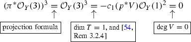 .
. -

 .
.
Before describing the other two terms we need to have a better understanding of E. The ideal \(\mathcal {J}_C\) of C corresponds to the graded ideal I of \({{\,\mathrm{{Sym}}\,}}V\) generated by the degree 1 ”monomials” \(\mathcal {O}_T(1) \oplus \mathcal {O}_T(1)\). Hence, the sheaf \(\mathcal {J}_C/\mathcal {J}^2_C\) corresponds to the rank 2 locally free graded module over \({{\,\mathrm{{Sym}}\,}}\left( \mathcal {O}_T(-2) \right) \) generated again by \(\mathcal {O}_T(1) \oplus \mathcal {O}_T(1)\) in degree 1, or equivalently to the rank 2 locally free graded module generated by \(\mathcal {O}_T(3) \oplus \mathcal {O}_T(3)\) in degree 0. Hence, \(E \cong \mathbb {P}W\), for \(W:=\mathcal {O}_C(3)\oplus \mathcal {O}_C(3)\), and \(\mathcal {O}_E(-E) \cong \mathcal {O}_{\mathbb {P}W}(1)\). In particular, the natural map \(\mathbb {P}W \rightarrow C\) can be identified with \(\pi |_E :\mathbb {P}^1\times C\rightarrow C\cong \mathbb {P}^1\), and \(\mathcal {O}_{\mathbb {P}W}(1)\equiv D+3F\) (see [62, Lemma II.7.9]), where D and F are the horizontal and the vertical rulings of E over C. We have:
-
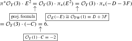
-
\(E^3=(-D-3F)^2=6\).

Wrapping up, we obtain
Example 12.2
In this example we exhibit a family \(f : X \rightarrow T\) of smooth degree 8 del Pezzo surfaces over a curve such that \(\deg \lambda _f>0\), or equivalently \((-K_{X/T})^3<0\), but \(-K_{X/T}\) is big. So, the statement \((-K_{X/T})^3<0\) is a negativity condition independent of \(-K_{X/T}\) being big or not. However, let us also note that there is one missing piece of our example: it is a family of non-K-semi-stable Fano varieties, although we suspect that a K-semi-stable one exists also.
Modify Example 12.1 replacing V with its dual; so we take \(V=\mathcal {O}_T(2)\oplus \mathcal {O}_T(-1)\oplus \mathcal {O}_T(-1)\) and we blow-up the curve defined by the quotient \(V\rightarrow \mathcal {O}_{\mathbb {P}^1}(2)\). In this case, \(\deg \lambda _{f}=12>0\). However, \(-K_{X/T}\) is still big. Indeed, write \(V=\mathcal {L}\oplus \mathcal {K}\oplus \mathcal {M}\), where \(\mathcal {L}=\mathcal {O}_T(2)\) and \(\mathcal {K}=\mathcal {M}=\mathcal {O}_T(-1)\). Then for every integer \(m>0\):

As \(\mathcal {I}_C\) is generated in \({{\,\mathrm{{Sym}}\,}}V\) by \(\mathcal {K}\oplus \mathcal {M}\), we obtain that
To show that \(-K_{X/T}\) is big, it is enough to prove that \(\displaystyle \lim _{m \rightarrow \infty } \frac{h^0( -mK_{X/T})}{m^3}>0\). Equation (12.2.a) yields:
Hence,
So, we showed indeed that \(-K_{X/T}\) is big, and we even computed that \({{\,\mathrm{{vol}}\,}}(-K_{X/T}) = 12\) (a coincidence with the previous number 12 above).
Example 12.3
Here we give an example of a family \(f : X \rightarrow T\) of smooth Del-Pezzo surfaces of degree 6 such that \(\delta _{X_t}=1\) for all closed point \(t \in T\), \(\deg \lambda _{f}=0\) but \(-K_{X/T}\) not nef. This shows that the hypothesis \(\delta >1\) in Theorem 1.20 is necessary.
For this, we modify Example 12.1 in two respects:
-
(a)
We take V to be the dual vector bundle, that is, \(V:=\mathcal {O}_T(2)\oplus \mathcal {O}_T(-1)\oplus \mathcal {O}_T(-1)\).
-
(b)
Instead of one curve, we blow up 3 curves. That is, we set \(X:= {{\,\mathrm{{Bl}}\,}}_{C_1, C_2, C_3} Y\), where \(C_i\) is the curve defined by the quotient \(V \rightarrow \mathcal {L}_i\), where \(\mathcal {L}_i\) is the i-th direct summand of V.
Let \(E_i\), \(F_i\) and \(W_i\) (and for \(i=1\) also \(D_1\)) to be defined for each \(C_i\) as E, F and W (and for \(i=1\) also D) was defined for C in Example 12.1. We do not define \(D_i\) also as in Example 12.1 because for \(i=2,3\), \(W_i = \mathcal {O}_{C_i} \oplus \mathcal {O}_{C_i}(3)\), so \(E_2, E_3 \not \cong \mathbb {P}^1 \times \mathbb {P}^1\). Instead, for \(i=2,3\), set \(D_i\) to be the divisor class of \(\mathcal {O}_{\mathbb {P}W_i}(1)\).
Note that the \(E_i\) are disjoint, and hence any intersection product involving different \(E_i\) is automatically 0. We write out below the computations where the result is different than in Example 12.1, where \(i=2\) or 3:
-
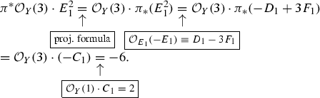
-
\(E^3_1=(-D_1+3F_1)^2=-6\).
-
\(\pi ^*\mathcal {O}_{Y}(3)\cdot E^2_i= \mathcal {O}_{Y}(3)\cdot \pi _*(E^2_i) = \mathcal {O}_{Y}(3)\cdot \pi _*(-D_i) =\mathcal {O}_{Y}(3)\cdot (- C_i)=3.\)
-
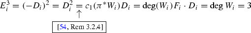 .
.

 .
.Set \(E:=E_1 + E_2 + E_3\). Then, we conclude that
The fibres of f are smooth del Pezzo surfaces of degree 6, they are well-known to be K-poly-stable (so, in particular, K-semi-stable), but they are not uniformly K-stable because they have a positive dimensional automorphism group. The delta invariant is thus equal to 1 (e.g., Corollary 4.9). Furthermore, for \(i=2,3\):
Hence, \(-K_{X/T}|_{E_i}\) is not nef, and then also \(-K_{X/T}\) is not nef.
Example 12.4
In this example, for each choice of an integer \(d>0\) we exhibit families \(f: X \rightarrow T\) of uniformly K-stable del Pezzo surfaces of degree 4 over a smooth projective curve. In this situation, Theorem 1.9.(a) tells us that \(\deg \lambda _f>0\), or equivalently \((-K_{X/T})^3<0\). So, one would expect \(-K_{X/T}\) to have only a few sections. Here, we show that both the expected and the unexpected behavior can happen. More precisely, \(|-K_{X/T}|_{\mathbb {Q}}= \emptyset \) for \(d>3\), and \(\kappa (-K_{X/T})\ge 1\) for \(d=1\).
Let \(p_1,\dots ,p_4\) be four points in \(\mathbb {P}^2\) in general position, and denote by \(L_{ij}\) the line trough \(p_i\) and \(p_j\). Let \(\iota :T\rightarrow \mathbb {P}^2\) be a degree d smooth curve in \(\mathbb {P}^2\) which avoids the four points. Let \(\Gamma \cong T\) be the graph of \(\iota \) in \(\mathbb {P}^2\times T\), and let \(T_i\) be the curve \(\{p_i\}\times T\) in \(\mathbb {P}^2\times T\). We want to look at the blow-up \(\pi :Y\rightarrow \mathbb {P}^2\times T\) of \(\Gamma \) and \(T_i\), for \(i=1,\dots , 4\). Denote by \(g:Y\rightarrow T\) the natural projection.
The family \(g:Y\rightarrow T\) is generically a family of degree 4 smooth del Pezzo surfaces of maximal variation. The only exception is at the points \(t \in T\) where \(\iota (T)\) intersects one of the lines \(L_{ij}\). In these cases, \(Y_t = {{\,\mathrm{{Bl}}\,}}_{p_1,p_2,p_3,p_4,p}\mathbb {P}^2\), where p lies on \(L_{ij}\). In particular, \(-K_{Y_t}\) is big and semi-ample, and there is a unique curve C for which \(C \cdot -K_{Y_t} =0\): the proper transform of \(L_{ij}\). The anti-canonical model is the contraction of \(L_{ij}\) to an \(A_1\) singularity, so in particular it has canonical singularities.
Let \(f:X\rightarrow T\) be the relative anti-canonical model of g (remark that \(R^ig_*(-mK_{Y/T})=0\) for \(i>0\) and m big enough, by Kawamata-Viehweg vanishing theorem, so we do have base change). The family f satisfies the hypotheses of Theorem 1.9(a), so \(\deg \lambda _f>0\).
We show that, if \(d>3\), then \(|-K_{X/T}|_{\mathbb {Q}}=\emptyset \) and if \(d=1\), then \(\kappa (-K_{X/T}) \ge 1\). In either case the crucial remark is that \(H^0(X,-mK_{X/T})\) can be identified with the subspace of\(H^0(\mathbb {P}^2 \times T, \mathcal {O}_{\mathbb {P}^2 \times T}(3m)) \cong H^0(\mathbb {P}^2, \mathcal {O}_{\mathbb {P}^2}(3m))\) which vanish along \(\iota (T)\) and \(p_i\) with multiplicity at least m. Hence:
-
If \(d>3\), then there are no such sections, as d is exactly the degree of \(\iota (T)\).
-
If \(d=1\), then \(\iota (T)\) is a line L. So, \(|-K_{X/T}|\) is the set of cubics C on \(\mathbb {P}^2\) such that C goes through \(p_i\) and \({{\,\mathrm{{Supp}}\,}}C\) contains L. Hence, \(C = L + C'\), where \(C'\) is a conic through \(p_i\). There is a one parameter family of such conics.
Notes
This conjecture has been proved in [125], published after the first version of this paper has appeared.
References
Alexeev, V., Hacon, C., Kawamata, Y.: Termination of (many) 4-dimensional log flips. Invent. Math. 168(2), 433–448 (2007)
Alper, J., Blum, H., Halpern-Leistner, D., Xu, C.: Reductivity of the automorphism group of K-polystable fano varieties. To appear in Invent, Math (2019)
Alper, J., Halpern-Leistner, D., Heinloth, J.: Existence of moduli spaces for algebraic stacks, arXiv:1812.01128 (2018)
Alper, J.: Good moduli spaces for Artin stacks. Ann. Inst. Fourier (Grenoble) 63(6), 2349–2402 (2013)
Arezzo, C., Ghigi, A., Pirola, G.P.: Symmetries, quotients and Kähler-Einstein metrics. J. Reine Angew. Math. 591, 177–200 (2006)
Ascher, K., Bejleri, D.: Moduli of weighted stable elliptic surfaces and invariance of log plurigenera, arXiv:1702.06107 (2017)
Barja, M.A., Stoppino, L.: Stability conditions and positivity of invariants of fibrations, Algebraic and complex geometry, Springer Proc. Math. Stat., vol. 71, Springer, Cham, (2014), pp. 1–40
Berman, R., Boucksom, S., Jonsson, M.: A variational approach to the Yau-Tian-Donaldson conjecture, arXiv:1509.04561 (2015)
Berman, R.J., Guenancia, H.: Kähler–Einstein metrics on stable varieties and log canonical pairs. Geom. Funct. Anal. 24(6), 1683–1730 (2014)
Birkar, C.: Existence of log canonical flips and a special LMMP, Publ. Math. Inst. Hautes Études Sci. 325–368 (2012)
Birkar, C.: Singularities of linear systems and boundedness of Fano varieties, arXiv:1609.05543 (2016)
Birkar, C.: Ascending chain condition for log canonical thresholds and termination of log flips. Duke Math. J. 136(1), 173–180 (2007)
Birkar, C.: On termination of log flips in dimension four. Math. Ann. 346(2), 251–257 (2010)
Birkar, C.: Anti-pluricanonical systems on Fano varieties. Ann. Math. (2) 190(2), 345–463 (2019)
Birkar, C., Cascini, P., Hacon, C.D., McKernan, J.: Existence of minimal models for varieties of log general type. J. Am. Math. Soc. 23(2), 405–468 (2010)
Blum, H., Liu, Y., Xu, C.: Openness of k-semistability for fano varieties, arXiv:1907.02408 (2019)
Blum, H., Liu, Y.: Openness of uniform k-stability in families of \(\mathbb{Q}\)-fano varieties. To appear in Ann. Sci. Éc. Norm, Supér (2018)
Blum, H., Liu, Y.: The normalized volume of a singularity is lower semicontinuous, To appear in J. Eur. Math. Soc. (2018)
Blum, H.: Thesis, manuscript (2018)
Blum, H., Jonsson, M.: Thresholds, valuations, and K-stability. Adv. Math. 365, 107062 (2020)
Blum, H., Xu, C.: Uniqueness of \(\text{ K }\)-polystable degenerations of Fano varieties. Ann. Math. (2) 190(2), 609–656 (2019)
Boucksom, S., Demailly, J.-P., Păun, M., Peternell, T.: The pseudo-effective cone of a compact Kähler manifold and varieties of negative Kodaira dimension. J. Algebraic Geom. 22(2), 201–248 (2013)
Boucksom, S., Hisamoto, T., Jonsson, M.: Uniform K-stability, Duistermaat–Heckman measures and singularities of pairs. Ann. Inst. Fourier (Grenoble) 67(2), 743–841 (2017)
Boucksom, S., Hisamoto, T., Jonsson, M.: Uniform K-stability and asymptotics of energy functionals in Kähler geometry. J. Eur. Math. Soc. (JEMS) 21(9), 2905–2944 (2019)
Cheltsov, I.A., Shramov, K.A.: Log-canonical thresholds for nonsingular Fano threefolds. Uspekhi Mat. Nauk 63(5(383)), 73–180 (2008)
Chen, X., Donaldson, S., Sun, S.: Kähler–Einstein metrics on Fano manifolds. I: approximation of metrics with cone singularities. J. Am. Math. Soc. 28(1), 183–197 (2015)
Chen, X., Donaldson, S., Sun, S.: Kähler–Einstein metrics on Fano manifolds. II: limits with cone angle less than \(2\pi \). J. Am. Math. Soc. 28(1), 199–234 (2015)
Chen, X., Donaldson, S., Sun, S.: Kähler–Einstein metrics on Fano manifolds. III: limits as cone angle approaches \(2\pi \) and completion of the main proof. J. Am. Math. Soc. 28(1), 235–278 (2015)
Codogni, G.: Tits buildings and K-stability. Proc. Edinb. Math. Soc. 62(3), 799–815 (2019)
Codogni, G., Fanelli, A., Svaldi, R., Tasin, L.: Fano varieties in Mori fibre spaces. Int. Math. Res. Not. IMRN 7, 2026–2067 (2016)
Codogni, G., Fanelli, A., Svaldi, R., Tasin, L.: A note on the fibres of Mori fibre spaces. Eur. J. Math. 4, 859–878 (2018)
Conrad, B.: Grothendieck duality and base change. Lecture Notes in Mathematics, vol. 1750. Springer-Verlag, Berlin (2000)
Cornalba, M., Harris, J.: Divisor classes associated to families of stable varieties, with applications to the moduli space of curves. Ann. Sci. École Norm. Sup. (4) 21(3), 455–475 (1988)
de Fernex, T., Kollár, J., Xu, C.: The dual complex of singularities, Higher dimensional algebraic geometry—in honour of Professor Yujiro Kawamata’s sixtieth birthday, Adv. Stud. Pure Math., vol. 74, Math. Soc. Japan, Tokyo, 2017, pp. 103–129
Demailly, J.-P.: Singular Hermitian metrics on positive line bundles, Complex algebraic varieties (Bayreuth, : Lecture Notes in Math., vol. 1507. Springer, Berlin 1992, 87–104 (1990)
Dervan, R.: On K-stability of finite covers. Bull. Lond. Math. Soc. 48(4), 717–728 (2016)
Dervan, R.: Uniform stability of twisted constant scalar curvature Kähler metrics. Int. Math. Res. Not. IMRN 15, 4728–4783 (2016)
Ding, W.Y., Tian, G.: Kähler-Einstein metrics and the generalized Futaki invariant. Invent. Math. 110(2), 315–335 (1992)
Donaldson, S.K.: Lower bounds on the Calabi functional. J. Differ. Geom. 70(3), 453–472 (2005)
Durrett, R.: Probability: Theory and Examples. Cambridge Series in Statistical and Probabilistic Mathematics, vol. 31, 4th edn. Cambridge University Press, Cambridge (2010)
Fine, J., Ross, J.: A note on positivity of the CM line bundle. Int. Math. Res. Not. (2006), Art. ID 95875, 14
Flips and abundance for algebraic threefolds: Société Mathématique de France, Paris, 1992, Papers from the Second Summer Seminar on Algebraic Geometry held at the University of Utah, Salt Lake City, Utah, August 1991. Astérisque No. 211, (1992)
Fujiki, A., Schumacher, G.: The moduli space of extremal compact Kähler manifolds and generalized Weil–Petersson metrics. Publ. Res. Inst. Math. Sci. 26(1), 101–183 (1990)
Fujino, O.: Introduction to the log minimal model program for log canonical pairs, arXiv:0907.1506 (2009)
Fujino, O.: Semipositivity theorems for moduli problems, preprint, https://www.math.kyoto-u.ac.jp/~fujino/semi-positivity7.pdf (2012)
Fujita, T.: On Kähler fiber spaces over curves. J. Math. Soc. Jpn. 30(4), 779–794 (1978)
Fujita, K.: Examples of K-unstable Fano manifolds with the Picard number 1. Proc. Edinb. Math. Soc. (2) 60(4), 881–891 (2017)
Fujita, K.: Optimal bounds for the volumes of Kähler–Einstein Fano manifolds. Am. J. Math. 140(2), 391–414 (2018)
Fujita, K.: Openness results for uniform K-stability. Math. Ann. 373(3–4), 1529–1548 (2019)
Fujita, K.: Uniform K-stability and plt blowups of log Fano pairs. Kyoto J. Math. 59(2), 399–418 (2019)
Fujita, K.: A valuative criterion for uniform K-stability of \(\mathbb{Q}\)-Fano varieties. J. Reine Angew. Math. 751, 309–338 (2019)
Fujita, K., Odaka, Y.: On the K-stability of Fano varieties and anticanonical divisors. Tohoku Math. J. (2) 70(4), 511–521 (2018)
Fulton, W.: Intersection theory, second ed., Ergebnisse der Mathematik und ihrer Grenzgebiete. 3. Folge. A Series of Modern Surveys in Mathematics [Results in Mathematics and Related Areas. 3rd Series. A Series of Modern Surveys in Mathematics], vol. 2, Springer-Verlag, Berlin, (1998)
Griffiths, P.A.: Periods of integrals on algebraic manifolds. III. Some global differential-geometric properties of the period mapping. Inst. Hautes Études Sci. Publ. Math. 38, 125–180 (1970)
Grothendieck, A.: Éléments de géométrie algébrique. IV. Étude locale des schémas et des morphismes de schémas. III, Inst. Hautes Études Sci. Publ. Math. 28, 255 (1966)
Grothendieck, A.: Éléments de géométrie algébrique. IV. Étude locale des schémas et des morphismes de schémas. II, Inst. Hautes Études Sci. Publ. Math. 24, 231 (1965)
Hacon, C.D., McKernan, J.: Existence of minimal models for varieties of log general type II. J. Am. Math. Soc. 23(2), 469–490 (2010)
Hacon, C.D., Xu, C.: Existence of log canonical closures. Invent. Math. 192(1), 161–195 (2013)
Harder, G., Narasimhan, M.S.: On the cohomology groups of moduli spaces of vector bundles on curves. Math. Ann. 212, 215–248 (1974/75)
Hartshorne, R.: Residues and duality, Lecture notes of a seminar on the work of A. Grothendieck, given at Harvard 1963/64. With an appendix by P. Deligne. Lecture Notes in Mathematics, No. 20, Springer, Berlin (1966)
Hartshorne, R.: Algebraic Geometry. Graduate Texts in Mathematics, No. 52. Springer, New York (1977)
Hartshorne, R.: Stable reflexive sheaves. Math. Ann. 254(2), 121–176 (1980)
Jiang, C.: Boundedness of \(\mathbb{Q}\)-Fano varieties with degrees and alpha-invariants bounded from below, to appear in Annales scientifiques de l’ENS (2018)
Jiang, C.: Boundedness of threefolds of fano type with mori fibration structures, arXiv:1601.02194 (2016)
Kawamata, Y.: Characterization of abelian varieties. Compos. Math. 43(2), 253–276 (1981)
Kawamata, Y.: Unobstructed deformations. A remark on a paper of Z. Ran: Deformations of manifolds with torsion or negative canonical bundle. J. Algebraic Geom. 1(2), 183–190 (1992)
Keel, S., Matsuki, K., McKernan, J.: Log abundance theorem for threefolds. Duke Math. J. 75(1), 99–119 (1994)
Knudsen, F.F., Mumford, D.: The projectivity of the moduli space of stable curves. I. Preliminaries on “det” and “Div”. Math. Scand. 39(1), 19–55 (1976)
Kollár, J., Mori, S.: Birational geometry of algebraic varieties, Cambridge Tracts in Mathematics, vol. 134, Cambridge University Press, Cambridge, (1998), With the collaboration of C. H. Clemens and A. Corti, Translated from the 1998 Japanese original
Kollár, J.: Families of varieties of general type, http://web.math.princeton.edu/~kollar/book/modbook20170720-hyper.pdf (2014)
Kollár, J.: Rational curves on algebraic varieties, Ergebnisse der Mathematik und ihrer Grenzgebiete. 3. Folge. A Series of Modern Surveys in Mathematics [Results in Mathematics and Related Areas. 3rd Series. A Series of Modern Surveys in Mathematics], vol. 32, Springer-Verlag, Berlin (1996)
Kollár, J.: Subadditivity of the Kodaira dimension: fibers of general type, Algebraic geometry, Sendai: Adv. Stud. Pure Math., vol. 10. North-Holland, Amsterdam 1987, 361–398 (1985)
Kollár, J.: Projectivity of complete moduli. J. Differ. Geom. 32(1), 235–268 (1990)
Kollár, J., Miyaoka, Y., Mori, S.: Rational connectedness and boundedness of Fano manifolds. J. Differ. Geom. 36(3), 765–779 (1992)
Kovács, S.J., Patakfalvi, Zs: Projectivity of the moduli space of stable log-varieties and subadditivity of log-Kodaira dimension. J. Am. Math. Soc. 30(4), 959–1021 (2017)
Lazarsfeld, R.: Positivity in algebraic geometry. II, Ergebnisse der Mathematik und ihrer Grenzgebiete. 3. Folge. A Series of Modern Surveys in Mathematics [Results in Mathematics and Related Areas. 3rd Series. A Series of Modern Surveys in Mathematics], vol. 49, Springer, Berlin. Positivity for vector bundles, and multiplier ideals (2004)
Lazarsfeld, R.: Positivity in algebraic geometry. I, Ergebnisse der Mathematik und ihrer Grenzgebiete. 3. Folge. A Series of Modern Surveys in Mathematics [Results in Mathematics and Related Areas. 3rd Series. A Series of Modern Surveys in Mathematics], vol. 48, Springer, Berlin. Classical setting: line bundles and linear series (2004)
Li, G., Tian, C., Wang, F.: On Yau-Tian-Donaldson conjecture for singular Fano varieties. arXiv:1711.09530 (2017)
Li, C., Liu, Y.: Kähler–einstein metrics and volume minimization. Adv. Math. 341, 440–492 (2019)
Li, C., Wang, X., Xu, C.: Quasi-projectivity of the moduli space of smooth Kähler-Einstein Fano manifolds. Ann. Sci. Éc. Norm. Supér. (4) 51(3), 739–772 (2018)
Li, C., Wang, X., Xu, C.: On the proper moduli spaces of smoothable Kähler–Einstein Fano varieties. Duke Math. J. 168(8), 1387–1459 (2019)
Liu, Y.: The volume of singular Kähler–Einstein Fano varieties. Compos. Math. 154(6), 1131–1158 (2018)
Liu, Y., Xu, C.: K-stability of cubic threefolds. Duke Math. J. 168(11), 2029–2073 (2019)
Mumford, D., Fogarty, J., Kirwan, F.: Geometric invariant theory, third ed., Ergebnisse der Mathematik und ihrer Grenzgebiete (2) [Results in Mathematics and Related Areas (2)], vol. 34, Springer-Verlag, Berlin (1994)
Nakamaye, M.: Stable base loci of linear series. Math. Ann. 318(4), 837–847 (2000)
Odaka, Y.: The Calabi conjecture and K-stability. Int. Math. Res. Not. IMRN 10, 2272–2288 (2012)
Odaka, Y.: The GIT stability of polarized varieties via discrepancy. Ann. Math. (2) 177(2), 645–661 (2013)
Odaka, Y.: Compact moduli spaces of Kähler–Einstein Fano varieties. Publ. Res. Inst. Math. Sci. 51(3), 549–565 (2015)
Odaka, Y., Okada, T.: Birational superrigidity and slope stability of Fano manifolds. Math. Z. 275(3–4), 1109–1119 (2013)
Odaka, Y., Sano, Y.: Alpha invariant and K-stability of \(\mathbb{Q}\)-Fano varieties. Adv. Math. 229(5), 2818–2834 (2012)
Odaka, Y., Sun, S.: Testing log K-stability by blowing up formalism. Ann. Fac. Sci. Toulouse Math. (6) 24(3), 505–522 (2015)
Odaka, Y., Xu, C.: Log-canonical models of singular pairs and its applications. Math. Res. Lett. 19(2), 325–334 (2012)
Odaka, Y., Spotti, C., Sun, S.: Compact moduli spaces of del Pezzo surfaces and Kähler-Einstein metrics. J. Differ. Geom. 102(1), 127–172 (2016)
Pardini, R.: The Severi inequality \(K^2\ge 4\chi \) for surfaces of maximal Albanese dimension. Invent. Math. 159(3), 669–672 (2005)
Park, J., Won, J.: K-stability of smooth del Pezzo surfaces. Math. Ann. 372(3–4), 1239–1276 (2018)
Patakfalvi, Zs., Schwede, K., Zhang, W.: \(F\)-singularities in families, arXiv:1305.1646 (2013)
Patakfalvi, Z., Xu, C.: Ampleness of the CM line bundle on the moduli space of canonically polarized varieties. Algebraic Geometry 4 (2017)
Patakfalvi, Zs: Semi-positivity in positive characteristics. Ann. Sci. Éc. Norm. Supér. (4) 47(5), 991–1025 (2014)
Patakfalvi, Zs: Semi-negativity of Hodge bundles associated to du bois families. J. Pure Appl. Algebra 219, 5387–5393 (2015)
Paul, S.T., Tian, G.: CM stability and the generalized Futaki invariant II. arXiv:math/0606505 (2006)
Paul, S.T., Tian, G.: CM stability and the generalized Futaki invariant II. Astérisque 2009(328), 339–354 (2010)
Phong, D.H., Ross, J., Sturm, J.: Deligne pairings and the Knudsen–Mumford expansion. J. Differ. Geom. 78(3), 475–496 (2008)
Posva, Q.: Positivity of the CM line bundle for K-stable log fanos, arXiv:1910.12623 (2019)
Ran, Z.: Deformations of manifolds with torsion or negative canonical bundle. J. Algebraic Geom. 1(2), 279–291 (1992)
Sano, T.: On deformations of \(\mathbb{Q}\)-Fano 3-folds. J. Algebraic Geom. 25(1), 141–176 (2016)
Simpson, C.T.: Higgs bundles and local systems. Inst. Hautes Études Sci. Publ. Math. 75, 5–95 (1992)
Spotti, C., Sun, S.: Explicit Gromov–Hausdorff compactifications of moduli spaces of Kähler–Einstein Fano manifolds. Pure Appl. Math. Q 13(3), 477–515 (2017)
Spotti, C., Sun, S., Yao, C.: Existence and deformations of Kähler–Einstein metrics on smoothable \(\mathbb{Q}\)-Fano varieties. Duke Math. J. 165(16), 3043–3083 (2016)
Stacks Project, http://stacks.math.columbia.edu
Stibitz, C., Zhuang, Z.: K-stability of birationally superrigid Fano varieties. Compos. Math. 155(9), 1845–1852 (2019)
Székelyhidi, G.: Filtrations and test-configurations. Math. Ann. 362(1–2), 451–484 (2015). With an appendix by Sebastien Boucksom
Tian, G.: On Kähler–Einstein metrics on certain Kähler manifolds with \(C_1(M)>0\). Invent. Math. 89(2), 225–246 (1987)
Tian, G.: On Calabi’s conjecture for complex surfaces with positive first Chern class. Invent. Math. 101(1), 101–172 (1990)
Tian, G.: Kähler–Einstein metrics with positive scalar curvature. Invent. Math. 130(1), 1–37 (1997)
Tian, G.: K-stability and Kähler–Einstein metrics. Commun. Pure Appl. Math. 68(7), 1085–1156 (2015)
Tian, G., Yau, S.-T.: Kähler–Einstein metrics on complex surfaces with \(C_1>0\). Commun. Math. Phys. 112(1), 175–203 (1987)
Viehweg, E.: Weak positivity and the additivity of the Kodaira dimension for certain fibre spaces, Algebraic varieties and analytic varieties (Tokyo: Adv. Stud. Pure Math., vol. 1. North-Holland, Amsterdam 1983, 329–353 (1981)
Viehweg, E.: Quasi-projective moduli for polarized manifolds, Ergebnisse der Mathematik und ihrer Grenzgebiete (3) [Results in Mathematics and Related Areas (3)], vol. 30. Springer, Berlin (1995)
Wang, X.: Height and GIT weight. Math. Res. Lett. 19(4), 909–926 (2012)
Wang, X., Xu, C.: Nonexistence of asymptotic GIT compactification. Duke Math. J. 163(12), 2217–2241 (2014)
Witt Nyström, D.: Test configurations and Okounkov bodies. Compos. Math. 148(6), 1736–1756 (2012)
Xiao, G.: Fibered algebraic surfaces with low slope. Math. Ann. 276(3), 449–466 (1987)
Xu, C.: A minimizing valuation is quasi-monomial. Ann. Math. (2) 191(3), 1003–1030 (2020)
Zhang, Q.: On projective manifolds with nef anticanonical bundles. J. Reine Angew. Math. 478, 57–60 (1996)
Zhuang, Z.: Birational superrigidity and K-stability of Fano complete intersections of index one (with an appendix written jointly with Charlie Stibitz), To appear on Duke Math. J. (2018)
Zhuang, Z.: Product theorem for K-stability. Adv. Math. 371, (2020)
Acknowledgements
We would like to thank the referee for the thorough and careful reading of the article, as well as for the many useful suggestions. This project gained significant momentum during the INdAM workshop ”Moduli of K-stable varieties; we thank INdAM for the organizational and financial support. We thank Harold Blum, Ruadhaí Dervan, Mattias Jonsson, Quentin Posva, Chenyang Xu and Maciej Zdanowicz for the many useful conversations and comments. The work of the second author was partially supported by the Swiss National Science Foundation grant #200021/169639. G.C. is funded by the MIUR Excellence Department Project, awarded to the Department of Mathematics, University of Rome, Tor Vergata, CUP E83C18000100006, and PRIN 2017 Advances in Moduli Theory and Birational Classification.
Funding
Open access funding provided by EPFL Lausanne.
Author information
Authors and Affiliations
Corresponding author
Additional information
Publisher's Note
Springer Nature remains neutral with regard to jurisdictional claims in published maps and institutional affiliations.
Appendix A Computations concerning the definition of the CM line bundle
Appendix A Computations concerning the definition of the CM line bundle
The following work is needed to prove the statements of Sect. 3. These are verifications of technical issues concerning the singular situation.
We need the following lemmas as we work with singular varieties, and hence Riemann-Roch computations do not work directly. It turns out that if the spaces are normal then singularities do not mess up any of the terms involving any of the definitions of the CM line bundle. However, in the non-normal situation, which we do not deal with in the present article, Lemma A.2 seems to suggest that one has to face extra difficulties.
Lemma A.1
Consider the following situation:
-
\(f : X \rightarrow T\) is a projective morphism to a normal quasi-projective variety (allowing \(T = {{\,\mathrm{{Spec}}\,}}k\)),
-
M is an f-ample \(\mathbb {Q}\)-divisor on X,
-
\(\mathcal {E}\) is a coherent sheaf on X, and
-
\(r \ge 0 \) is an integer such that \(\dim {{\,\mathrm{{Supp}}\,}}\mathcal {E}_t \le r\) for \(t \in T\) the generic point and \(\dim {{\,\mathrm{{Supp}}\,}}\mathcal {E}_t \le r+1\) for \(t \in T\) a codimension 1 point.
Then there are \(\mathbb {Q}\)-divisors \(D_i\) (resp. \(d_i \in \mathbb {Q}\)), determined uniquely up to \(\mathbb {Q}\)-linear equivalence (resp. determined uniquely), such that for all q divisible enough, if \(\dim T>0\), then
(resp. if \( T={{\,\mathrm{{Spec}}\,}}k\), then
Proof
In the case of \(T ={{\,\mathrm{{Spec}}\,}}k\), \(h^0 (X, \mathcal {O}_X(qM) \otimes \mathcal {E})\) equals the Hilbert polynomial for q divisible enough, and hence the statement follows. So, from now we assume that \(\dim T>0\).
Let \(s>0\) be an integer such that sM is relatively very ample. As the statement is for all q divisible enough, by replacing M with sM we may assume that M is relatively very ample and \(f_* \mathcal {O}_X(M)\) is locally free, in which case we will exhibit \(\mathbb {Z}\)-divisors \(D_i\). Furthermore, as the statement is about codimension 1 behavior over T, and \(T_{{{\,\mathrm{reg}\,}}}\) is a big open set of T, by replacing T with \(T_{{{\,\mathrm{reg}\,}}}\) we may assume that T is regular.
As M is relatively very ample, it induces an embedding \(\iota : X \hookrightarrow P:= {{\,\mathrm{{Proj}}\,}}_T f_* \mathcal {O}_X(M)\). Let \(\pi : P \rightarrow T\) be the natural morphism. As P is regular, \(\iota _* \mathcal {E}\) has a locally free resolution \(\mathcal {P}^\bullet \), which in particular is a perfect complex on P. Hence, for q divisible enough, the following holds (where, following [69], \(\det \) is the alternating tensor product of the determinants of the elements of a locally free resolution, which exists as T is regular):

Note that in the following lemma we do not assume any \(\mathbb {Q}\)-Cartier hypothesis on \(K_{X/T}\). Still, our intersection in (13.2.a) is well defined as M is \(\mathbb {Q}\)-Cartier.
Lemma A.2
Let \(f : X \rightarrow T\) be a surjective morphism from a normal projective variety of dimension \(n+d\) to a smooth variety of dimension \(d \ge 0\) with \(n \ge 1\), and let M be a \(\mathbb {Q}\)-Cartier f-ample divisor on X.
-
(a)
If \(\dim T>0\), then for all divisible enough integers \(q>0\),
$$\begin{aligned} c_1( f_* \mathcal {O}_X(qM)) = \frac{q^{n+1}}{(n+1)!} f_*\left( M^{n+1} \right) - \frac{q^n}{2 \cdot n!}f_* \left( K_{X/T} \cdot M^n \right) + p^{n-1}(q), \end{aligned}$$(13.2.a)where \(p^{n-1}(x)\) is polynomial of degree at most \(n-1\) with x as a variable and \(\mathbb {Q}\)-divisors as coefficients.
-
(b)
If \(T = {{\,\mathrm{{Spec}}\,}}k\), then \( \chi (X, qM) = \frac{M^n}{n!} q^{n} - \frac{K_X \cdot M^{n-1}}{2 (n-1)!} q^{n-1} + O(q^{n-2}). \)
In particular, if T is a curve and \(M^{n+1}>0\), then \(\deg f_* \mathcal {O}_X(qM)>0\) for all positive integers q divisible enough.
Proof
As Grothendieck-Riemann-Roch works directly only for smooth X (or also on locally complete intersection singularities, which does not include klt singularities with Cartier index greater than 1), we need to compare X with a resolution. Let \(\sigma : Z \rightarrow X\) be a resolution of singularities and set \(g:= f \circ \sigma \).
First, we claim that for all integers \(i>0\) and 1||q, in the respective cases:
-
(a)
\(\deg R^i g_* \mathcal {O}_Z(q \sigma ^* M) = p_i^{n-1}(q)\) for some polynomial \(p_i^{n-1}(x)\) of degree at most \(n-1\) and \(\mathbb {Q}\)-divisor coefficients, and
-
(b)
\( h^i (Z, q \sigma ^* M) = O(q^{n-2})\).
Indeed, fix an integer \(i>0\). There is a spectral sequence with \(E^2\)-terms \(R^p f_* ( \mathcal {O}_X(qM) \otimes R^r \sigma _* \mathcal {O}_Z )\) abutting to \(R^i g_* \mathcal {O}_Z(q \sigma ^* M) \) for \(i=p+r\). As M is f-ample and q is divisible enough, this spectral sequence degenerates. Therefore,
Then Lemma A.1 applied to \(\mathcal {E}:=R^i \sigma _* \mathcal {O}_Z \) concludes our claim, using that \( {{\,\mathrm{{Supp}}\,}}R^i \sigma _* \mathcal {O}_Z \) is contained in the non-normal locus, which is at most \(n-2\) dimensional in the generic fiber and at most \(n-1\) dimensional over the fibers over codimension 1 points.
Having shown our claim, in the \(\dim T>0\) case the statement of the proposition is shown by the following computation, which holds for every q divisible enough (so qM is f-very ample, Cartier and without higher cohomologies on the fibers):

In the case of \(T= {{\,\mathrm{{Spec}}\,}}k\), a similar computation concludes the proof:

\(\square \)
Remark A.3
In the situation of Lemma A.2, we also have that if T is a curve and \(M^{n+1}>0\), then M is big on X. Let us stress that M is not assumed to be nef on X, hence this does not follow directly from standard criteria such as [77, Theorem 2.2.14]. Indeed:

Proof of Proposition 3.7
Step 1: we may assume that T is smooth. If T is already smooth, there is nothing to prove, so assume that it is not smooth. Hence, by our assumptions, the fibers are normal and \({{\,\mathrm{{Supp}}\,}}\Delta \) does not contain any of the fibers. Take a resolution \(\tau : T' \rightarrow T\). Then, according to Sect. 2.4.1, in the respective cases,
-
(a)
\(f_{T'} : X_{T'} \rightarrow T'\) and \(L_{T'}\), and
-
(b)
\(f_{T'}: \left( X_{T'}, \Delta _{T'} \right) \rightarrow T'\) and \(L_{T'}\),
satisfy all our original assumptions, including that \(sL \sim -(K_{X/T} + \Delta )\) in the case of point (b) by Proposition 2.1.(a). We claim that \(\tau _* \lambda _{f_{T'},L_{T'}}= \lambda _{f,L}\) (resp. \(\tau _* \lambda _{f_{T'},\Delta _{T'}}= \lambda _{f,\Delta }\)). This is verified in the following computations, where \(\sigma : X_{T'} \rightarrow X\) is the induced morphism:
-
(a)
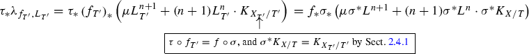
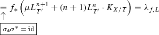 , and
, and -
(b)
$$\begin{aligned} \tau _* \lambda _{f_{T'},\Delta _{T'}}= & {} -\tau _* \left( f_{T'} \right) _* \left( -\left( K_{X_{T'}/T'} + \Delta _{T'}\right) ^{n+1} \right) \\= & {} - f_* \sigma _* \left( -\left( K_{X_{T'}/T'} + \Delta _{T'}\right) ^{n+1} \right) \\= & {} - f_* \left( -\left( K_{X/T} + \Delta \right) ^{n+1} \right) = \lambda _{f, \Delta }. \end{aligned}$$

 , and
, andHaving shown our claim, Step 1 follows. Indeed, if we prove, in the case of point (a), that \(s^n \lambda _{f_{T'},L_{T'}}= c_1(L_{{{\,\mathrm{{CM}}\,}},f_{T'}, sL_{T'}})\), then

The case of (b) is verbatim the same with \(s^n\), \(\lambda _{f, L}\) and \(L_{{{\,\mathrm{{CM}}\,}}, f, sL}\) replaced by \(-s^{n+1}\), \(\lambda _{f,\Delta }\) and \(\mathcal {M}_{n+1}\), respectively.
Step 2: The proof assuming that T is smooth. Set \(M_i:=c_1(\mathcal {M}_i)\). Taking into account that
according to Lemma A.2,
(where \(L= -(K_{X/T} + \Delta )\) in the case of point (b).) Hence, the next computation concludes the proof in the respective cases:
-
(a)
$$\begin{aligned} c_1(L_{{{\,\mathrm{{CM}}\,}}, f, sL})= & {} \left( n(n+1)+ \mu _{sL} \right) M_{n+1} -2 (n+1) M_n \\= & {} \left( n(n+1)+ \mu _{sL} \right) f_*((sL)^{n+1})\\&- 2(n+1) f_* \left( \frac{-K_{X/T} \cdot (sL)^n}{2 } + \frac{n (sL)^{n-1}}{2} \right) \\= & {} \frac{\mu _L}{s} s^{n+1} f_* L^{n+1} - s^n (n+1) f_* (K_{X/T}\cdot L^n) = s^n \lambda _{f,L} \end{aligned}$$
-
(b)
$$\begin{aligned} M_{n+1} = f_* \left( (-s(K_{X/T} + \Delta ))^{n+1} \right) = - s^{n+1} \lambda _{f, \lambda } \end{aligned}$$
\(\square \)
The next lemma is a technical statement used in Proposition 3.8.
Lemma A.4
Let \(h : V \rightarrow S\) be a flat n-relative dimensional morphism from a reduced projective scheme to a smooth projective curve, and let \(\mathcal {L}\) be an h-very ample line bundle on V. Let \(\pi : Z \rightarrow V\) be the normalization of V with \(g : Z \rightarrow S\) being the induced morphism, and assume also that \(\pi ^* \mathcal {L}\) is g-very ample. Then the \(n+1\)-th (so highest) Knudsen–Mumford coefficients of \(\mathcal {L}\) with respect to g (as in Notation 3.6) agrees with that of \(\pi ^* \mathcal {L}\).
Proof
Consider the exact sequence on V given by the normalization:

This yields a natural inclusion \(h_* \left( \mathcal {L}^q \right) \hookrightarrow g_* \left( \pi ^* \mathcal {L}^q \right) \). Hence, it is enough to prove that for q divisible enough, \(\deg h_* ( \mathcal {L}^q \otimes \mathcal {E}) = O(q^{n})\), which is given by Lemma A.1 as \(\dim {{\,\mathrm{{Supp}}\,}}\mathcal {E}\le n\). \(\square \)
Rights and permissions
Open Access This article is licensed under a Creative Commons Attribution 4.0 International License, which permits use, sharing, adaptation, distribution and reproduction in any medium or format, as long as you give appropriate credit to the original author(s) and the source, provide a link to the Creative Commons licence, and indicate if changes were made. The images or other third party material in this article are included in the article’s Creative Commons licence, unless indicated otherwise in a credit line to the material. If material is not included in the article’s Creative Commons licence and your intended use is not permitted by statutory regulation or exceeds the permitted use, you will need to obtain permission directly from the copyright holder. To view a copy of this licence, visit http://creativecommons.org/licenses/by/4.0/.
About this article

Cite this article
Codogni, G., Patakfalvi, Z. Positivity of the CM line bundle for families of K-stable klt Fano varieties. Invent. math. 223, 811–894 (2021). https://doi.org/10.1007/s00222-020-00999-y
Received:
Accepted:
Published:
Issue Date:
DOI: https://doi.org/10.1007/s00222-020-00999-y