Algebraic renormalisation of regularity structures

Abstract

We give a systematic description of a canonical renormalisation procedure of stochastic PDEs containing nonlinearities involving generalised functions. This theory is based on the construction of a new class of regularity structures which comes with an explicit and elegant description of a subgroup of their group of automorphisms. This subgroup is sufficiently large to be able to implement a version of the BPHZ renormalisation prescription in this context. This is in stark contrast to previous works where one considered regularity structures with a much smaller group of automorphisms, which lead to a much more indirect and convoluted construction of a renormalisation group acting on the corresponding space of admissible models by continuous transformations. Our construction is based on bialgebras of decorated coloured forests in cointeraction. More precisely, we have two Hopf algebras in cointeraction, coacting jointly on a vector space which represents the generalised functions of the theory. Two twisted antipodes play a fundamental role in the construction and provide a variant of the algebraic Birkhoff factorisation that arises naturally in perturbative quantum field theory.

1 Introduction

In a series of celebrated papers [10,11,12,13] Kuo-Tsai Chen discovered that, for any finite alphabet A, the family of iterated integrals of a smooth path $x:\mathbf{R}_+\rightarrow \mathbf{R}^A$ has a number of interesting algebraic properties. Writing for the tensor algebra on $\mathbf{R}^A$, which we identify with the space spanned by all finite words $\{(a_1\ldots a_n)\}_{n \ge 0}$ with letters in A, we define the family of functionals $\mathbb {X}_{s,t}$ on inductively by

$$\begin{aligned} \mathbb {X}_{s,t}(){\mathop {=}\limits ^{ \text{ def }}}1, \qquad \mathbb {X}_{s,t}(a_1\ldots a_{n}){\mathop {=}\limits ^{ \text{ def }}}\int _s^t \mathbb {X}_{s,u}(a_1\ldots a_{n-1}) \, \dot{x}_{a_n}(u) \, d u \end{aligned}$$

where $0\le s\le t$. Chen showed that this family yields for fixed s, t a character on endowed with the shuffle product, namely

(1.1)

which furthermore satisfies the flow relation

$$\begin{aligned} ( \mathbb {X}_{s,r}\otimes \mathbb {X}_{r,t}) \Delta \tau = \mathbb {X}_{s,t}\tau , \qquad s\le r\le t, \end{aligned}$$

where is the deconcatenation coproduct

$$\begin{aligned} \Delta (a_1\ldots a_n) = \sum _{k=0}^n (a_{1}\ldots a_{k}) \otimes (a_{k+1}\ldots a_{n})\;. \end{aligned}$$

In other words, we have a function which takes values in the characters on the algebra and satisfies the Chen relation

$$\begin{aligned} \mathbb {X}_{s,r}\star \mathbb {X}_{r,t}=\mathbb {X}_{s,t}, \qquad s\le r\le t, \end{aligned}$$

(1.2)

where $\star$ is the product dual to $\Delta$. Note that , endowed with the shuffle product and the deconcatenation coproduct, is a Hopf algebra.

These two remarkable properties do not depend explicitly on the differentiability of the path $(x_t)_{t\ge 0}$. They can therefore serve as an important tool if one wants to consider non-smooth paths and still build a consistent calculus. This intuition was at the heart of Terry Lyons’ definition [46] of a geometric rough path as a function satisfying the two algebraic properties above and with a controlled modulus of continuity, for instance of Hölder type

$$\begin{aligned} | \mathbb {X}_{s,t}(a_1 \ldots a_{n})|\le C |t-s|^{n\gamma }, \end{aligned}$$

(1.3)

with some fixed $\gamma >0$ (although the original definition involved rather a p-variation norm, which is natural in this context since it is invariant under reparametrisation of the path x, just like the definition of $\mathbb {X}$). Lyons realised that this setting would allow to build a robust theory of integration and of associated differential equations. For instance, in the case of stochastic differential equations of Stratonovich type

$$\begin{aligned} dX_t = \sigma (X_t) \circ dW_t\;, \end{aligned}$$

with $W:\mathbf{R}_+\rightarrow \mathbf{R}^d$ a d-dimensional Brownian motion and $\sigma :\mathbf{R}^d\rightarrow \mathbf{R}^d\otimes \mathbf{R}^d$ smooth, one can build rough paths $\mathbb {X}$ and ${\mathbb {W}}$ over X, respectively W, such that the map ${\mathbb {W}}\mapsto \mathbb {X}$ is continuous, while in general the map $W\mapsto X$ is simply measurable.

The Itô stochastic integration was included in Lyons’ theory although it can not be described in terms of geometric rough paths. A few years later Gubinelli [29] introduced the concept of a branched rough path as a function taking values in the characters of an algebra of rooted forests, satisfying the analogue of the Chen relation (1.2) with respect to the Grossman-Larsson $\star$-product, dual of the Connes-Kreimer coproduct, and with a regularity condition

$$\begin{aligned} | \mathbb {X}_{s,t}(\tau )|\le C |t-s|^{|\tau |\gamma } \end{aligned}$$

(1.4)

where $|\tau |$ counts the number of nodes in the forest $\tau$ and $\gamma >0$ is fixed. Again, this framework allows for a robust theory of integration and differential equations driven by branched rough paths. Moreover , endowed with the forest product and Connes-Kreimer coproduct, turns out to be a Hopf algebra.

The theory of regularity structures [32], due to the second named author of this paper, arose from the desire to apply the above ideas to (stochastic) partial differential equations (SPDEs) involving non-linearities of (random) space–time distributions. Prominent examples are the KPZ equation [23, 27, 31], the $\Phi ^4$ stochastic quantization equation [1, 7, 21, 32, 43, 45], the continuous parabolic Anderson model [26, 36, 37], and the stochastic Navier–Stokes equations [20, 53].

One apparent obstacle to the application of the rough paths framework to such SPDEs is that one would like to allow for the analogue of the map $s\mapsto \mathbb {X}_{s,t}\tau$ to be a space–time distribution for some . However, the algebraic relations discussed above involve products of such quantities, which are in general ill-defined. One of the main ideas of [32] was to replace the Hopf-algebra structure with a comodule structure: instead of a single space , we have two spaces and a coaction such that is a right comodule over the Hopf algebra . In this way, elements in the dual space of are used to encode the distributional objects which are needed in the theory, while elements of encode continuous functions. Note that admits neither a product nor a coproduct in general.

However, the comodule structure allows to define the analogue of a rough path as a pair: consider a distribution-valued continuous function

as well as a continuous function

The analogue of the Chen relation (1.2) is then given by

$$\begin{aligned} \gamma _{xy}\star \gamma _{yz}=\gamma _{xz}\;, \qquad \Pi _y \star \gamma _{yz} = \Pi _z\;, \end{aligned}$$

(1.5)

where the first $\star$-product is the convolution product on , while the second $\star$-product is given by the dual of the coaction $\Delta ^{\!+}$. This structure guarantees that all relevant expressions will be linear in the $\Pi _y$, so we never need to multiply distributions. To compare this expression to (1.2), think of for as being the analogue of $z \mapsto \mathbb {X}_{z,y}(\tau )$. Note that the algebraic conditions (1.5) are not enough to provide a useful object: analytic conditions analogous to (1.4) play an essential role in the analytical aspects of the theory. Once a model$\mathbb {X}= (\Pi ,\gamma )$ has been constructed, it plays a role analogous to that of a rough path and allows to construct a robust solution theory for a class of rough (partial) differential equations.

In various specific situations, the theory yields a canonical lift of any smoothened realisation of the driving noise for the stochastic PDE under consideration to a model $\mathbb {X}^\varepsilon$. Another major difference with what one sees in the rough paths setting is the following phenomenon: if we remove the regularisation as $\varepsilon \rightarrow 0$, neither the canonical model $\mathbb {X}^\varepsilon$ nor the solution to the regularised equation converge in general to a limit. This is a structural problem which reflects again the fact that some products are intrinsically ill-defined.

This is where renormalisation enters the game. It was already recognised in [32] that one should find a group $\mathfrak {R}$ of transformations on the space of models and elements $M_\varepsilon$ in $\mathfrak {R}$ in such a way that, when applying $M_\varepsilon$ to the canonical lift $\mathbb {X}^\varepsilon$, the resulting sequence of models converges to a limit. Then the theory essentially provides a black box, allowing to build maximal solutions for the stochastic PDE in question.

One aspect of the theory developed in [32] that is far from satisfactory is that while one has in principle a characterisation of $\mathfrak {R}$, this characterisation is very indirect. The methodology pursued so far has been to first make an educated guess for a sufficiently large family of renormalisation maps, then verify by hand that these do indeed belong to $\mathfrak {R}$ and finally show, again by hand, that the renormalised models converge to a limit. Since these steps did not rely on any general theory, they had to be performed separately for each new class of stochastic PDEs.

The main aim of the present article is to define an algebraic framework allowing to build regularity structures which, on the one hand, extend the ones built in [32] and, on the other hand, admit sufficiently many automorphisms (in the sense of [32, Def. 2.28]) to cover the renormalisation procedures of all subcritical stochastic PDEs that have been studied to date.

Moreover our construction is not restricted to the Gaussian setting and applies to any choice of the driving noise with minimal integrability conditions. In particular this allows to recover all the renormalisation procedures used so far in applications of the theory [32, 38,39,40, 42, 51]. It reaches however far beyond this and shows that the BPHZ renormalisation procedure belongs to the renormalisation group of the regularity structure associated to any class of subcritical semilinear stochastic PDEs. In particular, this is the case for the generalised KPZ equation which is the most natural stochastic evolution on loop space and is (formally!) given in local coordinates by

$$\begin{aligned} \partial _t u^\alpha = \partial _x^2 u^\alpha + \Gamma ^\alpha _{\beta \gamma }(u) \partial _x u^\beta \partial _x u^\gamma + \sigma _i^\alpha (u)\,\xi _i\;, \end{aligned}$$

(1.6)

where the $\xi _i$ are independent space–time white noises, $\Gamma ^\alpha _{\beta \gamma }$ are the Christoffel symbols of the underlying manifold, and the $\sigma _i$ are a collection of vector fields with the property that $\sum _i L_{\sigma _i}^2 = \Delta$, where $L_{\sigma }$ is the Lie derivative in the direction of $\sigma$ and $\Delta$ is the Laplace-Beltrami operator. Another example is given by the stochastic sine-Gordon equation [41] close to the Kosterlitz-Thouless transition. In both of these examples, the relevant group describing the renormalisation procedures is of very large dimension (about 100 in the first example and arbitrarily large in the second one), so that the verification “by hand” that it does indeed belong to the “renormalisation group” as done for example in [32, 39], would be impractical.

In order to describe the renormalisation procedure of SPDEs we introduce a new construction of an associated regularity structure, that will be called extended since it contains a new parameter which was not present in [32], the extended decoration. As above, this yields spaces , such that is a Hopf algebra and a right comodule over . The renormalisation procedure of distributions coded by is then described by another Hopf algebra and coactions and turning both and into left comodules over . This construction is, crucially, compatible with the comodule structure of over in the sense that $\Delta ^{\!-}_\mathrm {ex}$ and $\Delta ^{\!+}_\mathrm {ex}$ are in cointeraction in the terminology of [25], see formulae (3.48)–(5.26) and Remark 3.28 below. Once this structure is obtained, we can define renormalised models as follows: given a functional and a model $\mathbb {X}= (\Pi ,\gamma )$, we construct a new model $\mathbb {X}^g$ by setting

$$\begin{aligned} \gamma _{z\bar{z}}^g = (g \otimes \gamma _{z\bar{z}})\Delta ^{\!-}_\mathrm {ex}\;,\qquad \Pi _z^g = (g \otimes \Pi _z)\Delta ^{\!-}_\mathrm {ex}\;. \end{aligned}$$

The cointeraction property then guarantees that $\mathbb {X}^g$ satisfies again the generalised Chen relation (1.5). Furthermore, the action of on and is such that, crucially, the associated analytical conditions automatically hold as well.

All the coproducts and coactions mentioned above are a priori different operators, but we describe them in a unified framework as special cases of a contraction/extraction operation of subforests, as arising in the BPHZ renormalisation procedure/forest formula [3, 24, 35, 52]. It is interesting to remark that the structure described in this article is an extension of that previously described in [8, 14, 15] in the context of the analysis of B-series for numerical ODE solvers, which is itself an extension of the Connes-Kreimer Hopf algebra of rooted trees [16, 18] arising in the abovementioned forest formula in perturbative QFT. It is also closely related to incidence Hopf algebras associated to families of posets [49, 50].

There are however a number of substantial differences with respect to the existing literature. First we propose a new approach based on coloured forests; for instance we shall consider operations like

of colouring, extraction and contraction of subforests. Further, the abovementioned articles deal with two spaces in cointeraction, analogous to our Hopf algebras and , while our third space is the crucial ingredient which allows for distributions in the analytical part of the theory. Indeed, one of the main novelties of regularity structures is that they allow to study random distributional objects in a pathwise sense rather than through Feynman path integrals/correlation functions and the space encodes the fundamental bricks of this construction. Another important difference is that the structure described here does not consist of simple trees/forests, but they are decorated with multiindices on both their edges and their vertices. These decorations are not inert but transform in a non-trivial way under our coproducts, interacting with other operations like the contraction of sub-forests and the computation of suitable gradings.

In this article, Taylor sums play a very important role, just as in the BPHZ renormalisation procedure, and they appear in the coactions of both (the renormalisation) and (the recentering). In both operations, the group elements used to perform such operations are constructed with the help of a twisted antipode, providing a variant of the algebraic Birkhoff factorisation that was previously shown to arise naturally in the context of perturbative quantum field theory, see for example [16, 18, 19, 22, 30, 44].

In general, the context for a twisted antipode/Birkhoff factorisation is that of a group G acting on some vector space A which comes with a valuation. Given an element of A, one then wants to renormalise it by acting on it with a suitable element of G in such a way that its valuation vanishes. In the context of dimensional regularisation, elements of A assign to each Feynman diagram a Laurent series in a regularisation parameter $\varepsilon$, and the valuation extracts the pole part of this series. In our case, the space A consists of stationary random linear maps and we have two actions on it, by the group of characters of , corresponding to two different valuations. The renormalisation group is associated to the valuation that extracts the value of $\mathbf{E}(\varvec{\Pi }\tau )(0)$ for every homogeneous element of negative degree. The structure group on the other hand is associated to the valuations that extract the values $(\varvec{\Pi }\tau )(x)$ for all homogeneous elements of positive degree.

We show in particular that the twisted antipode related to the action of is intimately related to the algebraic properties of Taylor remainders. Also in this respect, regularity structures provide a far-reaching generalisation of rough paths, expanding Massimiliano Gubinelli’s investigation of the algebraic and analytic properties of increments of functions of a real variable achieved in the theory of controlled rough paths [28].

1.1 A general renormalisation scheme for SPDEs

Regularity Structures (RS) have been introduced [32] in order to solve singular SPDEs of the form

$$\begin{aligned} \partial _t u = \Delta u +F(u,\nabla u,\xi ) \end{aligned}$$

where $u=u(t,x)$ with $t\ge 0$ and $x\in \mathbf{R}^d$, $\xi$ is a random space–time Schwartz distribution (typically stationary and approximately scaling-invariant at small scales) driving the equation and the non-linear term $F(u,\nabla u,\xi )$ contains some products of distributions which are not well-defined by classical analytic methods. We write this equation in the customary mild formulation

$$\begin{aligned} u = G*(F(u,\nabla u,\xi )) \end{aligned}$$

(1.7)

where G is the heat kernel and we suppose for simplicity that $u(0,\cdot )=0$.

If we regularise the noise $\xi$ by means of a family of smooth mollifiers $(\varrho ^\varepsilon )_{\varepsilon >0}$, setting $\xi ^\varepsilon :=\varrho ^\varepsilon *\xi$, then the regularised PDE

$$\begin{aligned} u^\varepsilon = G*(F(u^\varepsilon ,\nabla u^\varepsilon ,\xi ^\varepsilon )) \end{aligned}$$

is well-posed under suitable assumptions on F. However, if we want to remove the regularisation by letting $\varepsilon \rightarrow 0$, we do not know whether $u^\varepsilon$ converges. The problem is that $\xi ^\varepsilon \rightarrow \xi$ in a space of distributions with negative (say) Sobolev regularity, and in such spaces the solution map $\xi ^\varepsilon \mapsto u^\varepsilon$ is not continuous.

The theory of RS allows to solve this problem for a class of equations, called subcritical. The general approach is as in Rough Paths (RP): the discontinuous solution map

is factorised as the composition of two maps:

where $(\mathscr {M},\mathrm{d})$ is a metric space that we call the space of models. The main point is that the map can be chosen in such a way that its is continuous, even though $\mathscr {M}$ is sufficiently large to allow for elements exhibiting a local scaling behaviour compatible with that of $\xi$. Of course this means that $\xi ^\varepsilon \mapsto {\mathbb {X}}^\varepsilon$ is discontinuous in general. In RP, the analogue of the model ${\mathbb {X}}^\varepsilon$ is the lift of the driving noise as a rough path, the map $\Phi$ is called the Itô-Lyons map, and its continuity (due to T. Lyons [46]) is the cornerstone of the theory. The construction of in the general context of subcritical SPDEs is one of the main results of [32].

The construction of $\Phi$, although a very powerful tool, does not solve alone the aforementioned problem, since it turns out that the most natural choice of ${\mathbb {X}}^\varepsilon$, which we call the canonical model, does in general not converge as we remove the regularisation by letting $\varepsilon \rightarrow 0$. It is necessary to modify, namely renormalise, the model ${\mathbb {X}}^\varepsilon$ in order to obtain a family $\hat{\mathbb {X}}^\varepsilon$ which does converge in $\mathscr {M}$ as $\varepsilon \rightarrow 0$ to a limiting model $\hat{\mathbb {X}}$. The continuity of $\Phi$ then implies that $\hat{u}^\varepsilon :=\Phi (\hat{\mathbb {X}}^\varepsilon )$ converges to some limit $\hat{u}:=\Phi (\hat{\mathbb {X}})$, which we call the renormalised solution to our equation, see Fig. 1. A very important fact is that $\hat{u}^\varepsilon$ is itself the solution of a renormalised equation, which differs from the original equation only by the presence of additional local counterterms, the form of which can be derived explicitly from the starting SPDE, see [2].

Fig. 1

In this figure we show the factorisation of the map $\xi ^\varepsilon \mapsto u^\varepsilon$ into $\xi ^\varepsilon \mapsto {\mathbb {X}}^\varepsilon \mapsto \Phi ({\mathbb {X}}^\varepsilon )=u^\varepsilon$. We also see that in the space of models $\mathscr {M}$ we have several possible lifts of $\xi ^\varepsilon \in {\mathcal {S}}'(\mathbf{R}^d)$, e.g. the canonical model ${\mathbb {X}}^\varepsilon$ and the renormalised model $\hat{\mathbb {X}}^\varepsilon$; it is the latter that converges to a model $\hat{\mathbb {X}}$, thus providing a lift of $\xi$. Note that $\hat{u}^\varepsilon =\Phi (\hat{\mathbb {X}}^\varepsilon )$ and $\hat{u}=\Phi (\hat{\mathbb {X}})$

The transformation ${\mathbb {X}}^\varepsilon \mapsto \hat{\mathbb {X}}^\varepsilon$ is described by the so-called renormalisation group. The main aim of this paper is to provide a general construction of the space of models $\mathscr {M}$ together with a group of automorphisms which allows to describe the renormalised model $\hat{\mathbb {X}}^\varepsilon =S_\varepsilon {\mathbb {X}}^\varepsilon$ for an appropriate choice of .

Starting with the $\varphi ^4_3$ equation and the Parabolic Anderson Model in [32], several equations have already been successfully renormalised with regularity structures [34, 36, 37, 39,40,41,42, 51]. In all these cases, the construction of the renormalised model and its convergence as the regularisation is removed are based on ad hoc arguments which have to be adapted to each equation. The present article, together with the companion “analytical” article [9] and the work [2], complete the general theory initiated in [32] by proving that virtually every¹ subcritical equation driven by a stationary noise satisfying some natural bounds on its cumulants can be successfully renormalised by means of the following scheme:

• Algebraic step: Construction of the space of models $(\mathscr {M},\mathrm{d})$ and renormalisation of the canonical model $\mathscr {M}\ni {\mathbb {X}}^\varepsilon \mapsto \hat{\mathbb {X}}^\varepsilon \in \mathscr {M}$, this article.

• Analytic step: Continuity of the solution map , [32].

• Probabilistic step: Convergence in probability of the renormalised model $\hat{\mathbb {X}}^\varepsilon$ to $\hat{\mathbb {X}}$ in $(\mathscr {M},\mathrm{d})$, [9].

• Second algebraic step: Identification of $\Phi (\hat{\mathbb {X}}^\varepsilon )$ with the classical solution map for an equation with local counterterms, [2].

We stress that this procedure works for very general noises, far beyond the Gaussian case.

1.2 Overview of results

We now describe in more detail the main results of this paper. Let us start from the notion of a subcritical rule. A rule, introduced in Definition 5.7 below, is a formalisation of the notion of a “class of systems of stochastic PDEs”. More precisely, given any system of equations of the type (1.7), there is a natural way of assigning to it a rule (see Sect. 5.4 for an example), which keeps track of which monomials (of the solution, its derivatives, and the driving noise) appear on the right hand side for each component. The notion of a subcritical rule, see Definition 5.14, translates to this general context the notion of subcriticality of equations which was given more informally in [32, Assumption 8.3].

Suppose now that we have fixed a subcritical rule. The first aim is to construct an associated space of models $\mathscr {M}^\mathrm {ex}$. The superscript ‘$\mathrm {ex}$’ stands for extended and is used to distinguish this space from the restricted space of models $\mathscr {M}$, see Definition 6.24, which is closer to the original construction of [32]. The space $\mathscr {M}^\mathrm {ex}$ extends $\mathscr {M}$ in the sense that there is a canonical continuous injection $\mathscr {M}\hookrightarrow \mathscr {M}^\mathrm {ex}$, see Theorem 6.33. The reason for considering this larger space is that it admits a large group of automorphisms in the sense of [32, Def. 2.28] which can be described in an explicit way. Our renormalisation procedure then makes use of a suitable subgroup which leaves $\mathscr {M}$ invariant. The reason why we do not describe its action on $\mathscr {M}$ directly is that although it acts by continuous transformations, it no longer acts by automorphisms, making it much more difficult to describe without going through $\mathscr {M}^\mathrm {ex}$.

To define $\mathscr {M}^\mathrm {ex}$, we construct a regularity structure in the sense of [32, Def. 2.1]. This is done in Sect. 5, see in particular Definitions 5.26–5.35 and Proposition 5.39. The corresponding structure group is constructed as the character group of a Hopf algebra , see (5.23), Proposition 5.34 and Definition 5.36. The vector space is a right-comodule over , namely there are linear operators

such that the identity

$$\begin{aligned} (\mathrm {id}\otimes \Delta ^{\!+}_\mathrm {ex})\Delta ^{\!+}_\mathrm {ex}=(\Delta ^{\!+}_\mathrm {ex}\otimes \mathrm {id})\Delta ^{\!+}_\mathrm {ex}\;, \end{aligned}$$

(1.8)

holds both between operators on and on . The fact that the two operators have the same name but act on different spaces should not generate confusion since the domain is usually clear from context. When it isn’t, as in (1.8), then the identity is assumed by convention to hold for all possible meaningful interpretations.

Next, the renormalisation group is defined as the character group of the Hopf algebra , see (5.23), Proposition 5.35 and Definition 5.36. The vector spaces and are both left-comodules over , so that acts on the left on and on . Again, this means that we have operators

such that

$$\begin{aligned} (\mathrm {id}\otimes \Delta ^{\!-}_\mathrm {ex})\Delta ^{\!-}_\mathrm {ex}=(\Delta ^{\!-}_\mathrm {ex}\otimes \mathrm {id})\Delta ^{\!-}_\mathrm {ex}. \end{aligned}$$

The action of on the corresponding dual spaces is given by

Crucially, these separate actions satisfy a compatibility condition which can be expressed as a cointeraction property, see (5.26) in Theorem 5.37, which implies the following relation between the two actions above:

(1.9)

see Proposition 3.33 and (5.27). This result is the algebraic linchpin of Theorem 6.16, where we construct the action of on the space $\mathscr {M}^\mathrm {ex}$ of models.

The next step is the construction of the space of smooth models of the regularity structure . This is done in Definition 6.7, where we follow [32, Def. 2.17], with the additional constraint that we consider smooth objects. Indeed, we are interested in the canonical model associated to a (regularised) smooth noise, constructed in Proposition 6.12 and Remark 6.13, and in its renormalised versions, namely its orbit under the action of , see Theorem 6.16.

Finally, we restrict our attention to a class of models which are random, stationary and have suitable integrability properties, see Definition 6.17. In this case, we can define a particular deterministic element of that gives rise to what we call the BPHZ renormalisation, by analogy with the corresponding construction arising in perturbative QFT [3, 24, 35, 52], see Theorem 6.18. We show that the BPHZ construction yields the unique element of such that the associated renormalised model yields a centered family of stochastic processes on the finite family of elements in with negative degree. This is the algebraic step of the renormalisation procedure.

This is the point where the companion analytical paper [9] starts, and then goes on to prove that the BPHZ renormalised model does converge in the metric $\mathrm{d}$ on $\mathscr {M}$, thus achieving the probabilistic step mentioned above and thereby completing the renormalisation procedure.

The BPHZ functional is expressed explicitly in terms of an interesting map that we call negative twisted antipode by analogy to [17], see Proposition 6.6 and (6.25). There is also a positive twisted antipode, see Proposition 6.3, which plays a similarly important role in (6.12). The main point is that these twisted antipodes encode in the compact formulae (6.12) and (6.25) a number of nontrivial computations.

How are these spaces and operators defined? Since the analytic theory of [32] is based on generalised Taylor expansions of solutions, the vector space is generated by a basis which codes the relevant generalised Taylor monomials, which are defined iteratively once a rule (i.e. a system of equations) is fixed. Definitions 5.8, 5.13 and 5.26 ensure that is sufficiently rich to allow one to rewrite (1.7) as a fixed point problem in a space of functions with values in our regularity structure. Moreover must also be invariant under the actions of . This is the aim of the construction in Sects. 2, 3 and 4, that we want now to describe.

The spaces which are constructed in Sect. 5 depend on the choice of a number of parameters, like the dimension of the coordinate space, the leading differential operator in the equation (the Laplacian being just one of many possible choices), the non-linearity, the noise. In the previous sections we have built universal objects with nice algebraic properties which depend on none of these choices, but for the dimension of the space, namely an (arbitrary) integer number d fixed once for all.

The spaces , and are obtained by considering repeatedly suitable subsets and suitable quotients of two initial spaces, called $\mathfrak {F}_1$ and $\mathfrak {F}_2$ and defined in and after Definition 4.1; more precisely, $\mathfrak {F}_1$ is the ancestor of and , while $\mathfrak {F}_2$ is the ancestor of . In Sect. 4 we represent these spaces as linearly generated by a collection of decorated forests, on which we can define suitable algebraic operations like a product and a coproduct, which are later inherited by , and (through other intermediary spaces which are called , and ). An important difference between and is that the former is linearly generated by a family of forests, while the latter is linearly generated by a family of trees; this difference extends to the algebra structure: is endowed with a forest product which corresponds to the disjoint union, while is endowed with a tree product whereby one considers a disjoint union and then identifies the roots.

The content of Sect. 4 is based on a specific definition of the spaces $\mathfrak {F}_1$ and $\mathfrak {F}_2$. In Sects. 2 and 3 however we present a number of results on a family of spaces $(\mathfrak {F}_i)_{i\in I}$ with $I\subset \mathbf{N}$, which are supposed to satisfy a few assumptions; Sect. 4 is therefore only a particular example of a more general theory, which is outlined in Sects. 2 and 3. In this general setting we consider spaces $\mathfrak {F}_i$ of decorated forests, and vector spaces ${\langle \mathfrak {F}_i\rangle }$ of infinite series of such forests. Such series are not arbitrary but adapted to a grading, see Sect. 2.3; this is needed since our abstract coproducts of Definition 3.3 contain infinite series and might be ill-defined if were to work on arbitrary formal series.

The family of spaces $(\mathfrak {F}_i)_{i\in I}$ are introduced in Definition 3.12 on the basis of families of admissible forests $\mathfrak {A}_i$, $i\in I$. If $(\mathfrak {A}_i)_{i\in I}$ satisfy Assumptions 1, 2, 3, 4, 5 and 6, then the coproducts $\Delta _i$ of Definition 3.3 are coassociative and moreover $\Delta _i$ and $\Delta _j$ for $i<j$ are in cointeraction, see (3.27). As already mentioned, the cointeraction property is the algebraic formula behind the fundamental relation (1.9) between the actions of and on . “Appendix A” contains a summary of the relations between the most important spaces appearing in this article, while “Appendix B” contains a symbolic index.

2 Rooted forests and bigraded spaces

Given a finite set S and a map $\ell :S \rightarrow \mathbf{N}$, we write

$$\begin{aligned} \ell ! {\mathop {=}\limits ^{ \text{ def }}}\prod _{x \in S} \ell (x)!\;, \end{aligned}$$

and we define the corresponding binomial coefficients accordingly. Note that if $\ell _1$ and $\ell _2$ have disjoint supports, then $(\ell _1 + \ell _2)! = \ell _1!\,\ell _2!$. Given a map $\pi :S \rightarrow \bar{S}$, we also define $\pi _\star \ell :\bar{S} \rightarrow \mathbf{N}$ by $\pi _\star \ell (x) = \sum _{y \in \pi ^{-1}(x)} \ell (y)$.

For $k,\ell :S \rightarrow \mathbf{N}$ we define

$$\begin{aligned} \left( {\begin{array}{c}k\\ \ell \end{array}}\right) {\mathop {=}\limits ^{ \text{ def }}}\prod _{x \in S}\left( {\begin{array}{c}k(x)\\ \ell (x)\end{array}}\right) \;, \end{aligned}$$

with the convention $\left( {\begin{array}{c}k\\ \ell \end{array}}\right) = 0$ unless $0\le \ell \le k$, which will be used throughout the paper. With these definitions at hand, one has the following slight reformulation of the classical Chu–Vandermonde identity.

Lemma 2.1

(Chu–Vandermonde) For every $k :S \rightarrow \mathbf{N}$, one has the identity

$$\begin{aligned} \sum _{\ell \,:\, \pi _\star \ell }\left( {\begin{array}{c}k\\ \ell \end{array}}\right) = \left( {\begin{array}{c}\pi _\star k\\ \pi _\star \ell \end{array}}\right) \;, \end{aligned}$$

where the sum runs over all possible choices of $\ell$ such that $\pi _\star \ell$ is fixed. $\square$

Remark 2.2

These notations are also consistent with the case where the maps k and $\ell$ are multi-index valued under the natural identification of a map $S \rightarrow \mathbf{N}^d$ with a map $S \times \{1,\ldots ,\infty \} \rightarrow \mathbf{N}$ given by $\ell (x)_i \leftrightarrow \ell (x,i)$.

2.1 Rooted trees and forests

Recall that a rooted tree T is a finite tree (a finite connected simple graph without cycles) with a distinguished vertex, $\varrho =\varrho _T$, called the root. Vertices of T, also called nodes, are denoted by $N=N_T$ and edges by $E=E_T\subset N^2$. Since we want our trees to be rooted, they need to have at least one node, so that we do not allow for trees with $N_T = \varnothing$. We do however allow for the trivial tree consisting of an empty edge set and a vertex set with only one element. This tree will play a special role in the sequel and will be denoted by $\bullet$. We will always assume that our trees are combinatorial meaning that there is no particular order imposed on edges leaving any given vertex.

Given a rooted tree T, we also endow $N_T$ with the partial order $\le$ where $w \le v$ if and only if w is on the unique path connecting v to the root, and we orient edges in $E_T$ so that if $(x,y) = (x \rightarrow y) \in E_T$, then $x \le y$. In this way, we can always view a tree as a directed graph.

Two rooted trees T and $T'$ are isomorphic if there exists a bijection $\iota :E_T \rightarrow E_{T'}$ which is coherent in the sense that there exists a bijection $\iota _N :N_T \rightarrow N_{T'}$ such that $\iota (x,y) = (\iota _N(x),\iota _N(y))$ for any edge $(x,y) \in e$ and such that the roots are mapped onto each other.

We say that a rooted tree is typed if it is furthermore endowed with a function $\mathfrak {t}:E_T \rightarrow \mathfrak {L}$, where $\mathfrak {L}$ is some finite set of types. We think of $\mathfrak {L}$ as being fixed once and for all and will sometimes omit to mention it in the sequel. In particular, we will never make explicit the dependence on the choice of $\mathfrak {L}$ in our notations. Two typed trees $(T,\mathfrak {t})$ and $(T',\mathfrak {t}')$ are isomorphic if T and $T'$ are isomorphic and $\mathfrak {t}$ is pushed onto $\mathfrak {t}'$ by the corresponding isomorphism $\iota$ in the sense that $\mathfrak {t}'\circ \iota = \mathfrak {t}$.

Similarly to a tree, a forestF is a finite simple graph (again with nodes $N_F$ and edges $E_F \subset N_F^2$) without cycles. A forest F is rooted if every connected component T of F is a rooted tree with root $\varrho _T$. As above, we will consider forests that are typed in the sense that they are endowed with a map $\mathfrak {t}:E_F \rightarrow \mathfrak {L}$, and we consider the same notion of isomorphism between typed forests as for typed trees. Note that while a tree is non-empty by definition, a forest can be empty. We denote the empty forest by either $\mathbf {1}$ or $\varnothing$.

Given a typed forest F, a subforest $A \subset F$ consists of subsets $E_A \subset E_F$ and $N_A \subset N_F$ such that if $(x,y) \in E_A$ then $\{x,y\}\subset N_A$. Types in A are inherited from F. A connected component of A is a tree whose root is defined to be the minimal node in the partial order inherited from F. We say that subforests A and B are disjoint, and write $A \cap B = \varnothing$, if one has $N_A \cap N_B = \varnothing$ (which also implies that $E_A\cap E_B = \varnothing$). Given two typed forests F, G, we write $F\sqcup G$ for the typed forest obtained by taking the disjoint union (as graphs) of the two forests F and G and adjoining to it the natural typing inherited from F and G. If furthermore $A \subset F$ and $B \subset G$ are subforests, then we write $A \sqcup B$ for the corresponding subforest of $F \sqcup G$.

We fix once and for all an integer $d\ge 1$, dimension of the parameter-space $\mathbf{R}^d$. We also denote by $\mathbf{Z}(\mathfrak {L})$ the free abelian group generated by $\mathfrak {L}$.

2.2 Coloured and decorated forests

Given a typed forest F, we want now to consider families of disjoint subforests of F, denoted by $(\hat{F}_i, i>0)$. It is convenient for us to code this family with a single function $\hat{F}:E_F \sqcup N_F \rightarrow \mathbf{N}$ as given by the next definition.

Definition 2.3

A coloured forest is a pair $(F,\hat{F})$ such that

• 1. $F = (E_F,N_F,\mathfrak {t})$ is a typed rooted forest

• 2. $\hat{F} :E_F \sqcup N_F \rightarrow \mathbf{N}$ is such that if $\hat{F}(e) \ne 0$ for $e=(x,y) \in E_F$ then $\hat{F}(x) = \hat{F}(y) = \hat{F}(e)$.

We say that $\hat{F}$ is a colouring of F. For $i > 0$, we define the subforest of F

$$\begin{aligned} \hat{F}_i = (\hat{E}_i, \hat{N}_i), \qquad \hat{E}_i =\hat{F}^{-1}(i)\cap E_F, \quad \hat{N}_i =\hat{F}^{-1}(i)\cap N_F, \end{aligned}$$

as well as $\hat{E} = \bigcup _{i > 0} \hat{E}_i$. We denote by $\mathfrak {C}$ the set of coloured forests.

The condition on $\hat{F}$ guarantees that every $\hat{F}_i$ is indeed a subforest of F for $i>0$ and that they are all disjoint. On the other hand, $\hat{F}^{-1}(0)$ is not supposed to have any particular structure and 0 is not counted as a colour.

Example 2.4

This is an example of a forest with two colours: red for 1 and blue for 2 (and black for 0)

We then have $\hat{F}_1= \hat{F}^{-1}(1) = A_1\sqcup A_3$ and $\hat{F}_2=\hat{F}^{-1}(2) = A_2\sqcup A_4$.

The set $\mathfrak {C}$ is a commutative monoid under the forest product

$$\begin{aligned} (F,\hat{F}) \cdot (G,\hat{G}) = (F\sqcup G,\hat{F}+ \hat{G})\;, \end{aligned}$$

(2.1)

where colouringss defined on one of the forests are extended to the disjoint union by setting them to vanish on the other forest. The neutral element for this associative product is the empty coloured forest $\mathbf {1}$.

We add now decorations on the nodes and edges of a coloured forest. For this, we fix throughout this article an arbitrary “dimension” $d \in \mathbf{N}$ and we give the following definition.

Definition 2.5

We denote by $\mathfrak {F}$ the set of all 5-tuples $(F,\hat{F},\mathfrak {n},\mathfrak {o},\mathfrak {e})$ such that

• 1. $(F,\hat{F})\in \mathfrak {C}$ is a coloured forest in the sense of Definition 2.3.

• 2. One has $\mathfrak {n}:N_F \rightarrow \mathbf{N}^d$

• 3. One has $\mathfrak {o}:N_F \rightarrow \mathbf{Z}^d\oplus \mathbf{Z}(\mathfrak {L})$ with $\text {supp}\mathfrak {o}\subset \text {supp}\hat{F}$.

• 4. One has $\mathfrak {e}:E_F \rightarrow \mathbf{N}^d$ with $\text {supp}\mathfrak {e}\subset \{e\in E_F :\, \hat{F}(e)=0\}=E_F\setminus \hat{E}$.

Remark 2.6

The reason why $\mathfrak {o}$ takes values in the space $\mathbf{Z}^d\oplus \mathbf{Z}(\mathfrak {L})$ will become apparent in (3.33) below when we define the contraction of coloured subforests and its action on decorations.

We identify $(F,\hat{F},\mathfrak {n},\mathfrak {o},\mathfrak {e})$ and $(F',\hat{F}',\mathfrak {n}',\mathfrak {o}',\mathfrak {e}')$ whenever F is isomorphic to $F'$, the corresponding isomorphism maps $\hat{F}$ to $\hat{F}'$ and pushes the three decoration functions onto their counterparts. We call elements of $\mathfrak {F}$decorated forests. We will also sometimes use the notation $(F,\hat{F})^{\mathfrak {n},\mathfrak {o}}_\mathfrak {e}$ instead of $(F,\hat{F},\mathfrak {n},\mathfrak {o},\mathfrak {e})$.

Example 2.7

Let consider the decorated forest $(F,\hat{F},\mathfrak {n},\mathfrak {o},\mathfrak {e})$ given by

In this figure, the edges in $E_F$ are labelled with the numbers from 1 to 13 and the nodes in $N_F$ with the letters $\{a,b,c,f,e,f,g,h,i,j,k,l,m,p\}$. We set $\hat{F}^{-1}(1)=\{b,d,e,j,k\}\sqcup \{3,4,9\}$ (red subforest), $\hat{F}^{-1}(2)=\{a,c,f,g,l,m\}\sqcup \{2,5,6,11,12\}$ (blue subforest), and on all remaining (black) nodes and edges $\hat{F}$ is set equal to 0. Every edge has a type $\mathfrak {t}\in \mathfrak {L}$, but only black edges have a possibly non-zero decoration $\mathfrak {e}\in \mathbf{N}^d$. All nodes have a decoration $\mathfrak {n}\in \mathbf{N}^d$, but only coloured nodes have a possibly non-zero decoration $\mathfrak {o}\in \mathbf{Z}^d\oplus \mathbf{Z}(\mathfrak {L})$.

Example 2.7 is continued in Examples 3.2, 3.4 and 3.5.

Definition 2.8

For any coloured forest $(F,\hat{F})$, we define an equivalence relation $\sim$ on the node set $N_F$ by saying that $x \sim y$ if x and y are connected in $\hat{E}$; this is the smallest equivalence relation for which $x \sim y$ whenever $(x,y) \in \hat{E}$.

Definition 2.8 will be extended to a decorated forest $(F,\hat{F},\mathfrak {n},\mathfrak {o},\mathfrak {e})$ in Definition 3.18 below.

Remark 2.9

We want to show the intuition behind decorated forests. We think of each $\tau =(F, \hat{F},\mathfrak {n},\mathfrak {o},\mathfrak {e})$ as defining a function on $(\mathbf{R}^d)^{N_F}$ in the following way. We associate to each type $\mathfrak {t}\in \mathfrak {L}$ a kernel $\varphi _\mathfrak {t}:\mathbf{R}^d\rightarrow \mathbf{R}$ and we define the domain

$$\begin{aligned} U_F{\mathop {=}\limits ^{ \text{ def }}}\left\{ x\in (\mathbf{R}^d)^{N_F} : \ x_v = x_w \quad \text {if} \quad v\sim w\right\} \;, \end{aligned}$$

where $\sim$ is the equivalence relation of Definition 2.8. Then we set ,

$$\begin{aligned} H_\tau (x_v, v\in N_{F}) {\mathop {=}\limits ^{ \text{ def }}}\prod _{v\in N_F} (x_v)^{\mathfrak {n}(v)} \prod _{e=(u,v)\in E_F\setminus \hat{E}} \partial ^{\mathfrak {e}(e)}\varphi _{\mathfrak {t}(e)}(x_u-x_v), \end{aligned}$$

(2.2)

where, for $x=(x^1,\ldots ,x^d)\in \mathbf{R}^d$, $n=(n^1,\ldots ,n^d)\in \mathbf{N}^d$ and

In this way, a decorated forest encodes a function: every node in $N_F/\sim$ represents a variable in $\mathbf{R}^d$, every uncoloured edge of a certain type $\mathfrak {t}$ a function $\varphi _{\mathfrak {t}(e)}$ of the difference of the two variables sitting at each one of its nodes; the decoration $\mathfrak {n}(v)$ gives a power of $x_v$ and $\mathfrak {e}(e)$ a derivative of the kernel $\varphi _{\mathfrak {t}(e)}$.

In this example the decoration $\mathfrak {o}$ plays no role; we shall see below that it allows to encode some additional information relevant for the various algebraic manipulations we wish to subject these functions to, see Remarks 3.7, 3.19, 5.38 and 6.26 below for further discussions.

Remark 2.10

Every forest $F=(N_F,E_F)$ has a unique decomposition into non-empty connected components. This property naturally extends to decorated forests $(F, \hat{F},\mathfrak {n},\mathfrak {o},\mathfrak {e})$, by considering the connected components of the underlying forest F and restricting the colouring $\hat{F}$ and the decorations $\mathfrak {n},\mathfrak {o},\mathfrak {e}$.

Remark 2.11

Starting from Sect. 4 we are going to consider a specific situation where there are only two colours, namely $\hat{F}\rightarrow \{0,1,2\}$; all examples throughout the paper are in this setting. However the results of Sects. 2 and 3 are stated and proved in the more general setting $\hat{F}\rightarrow \mathbf{N}$ without any additional difficulty.

2.3 Bigraded spaces and triangular maps

It will be convenient in the sequel to consider a particular category of bigraded spaces as follows.

Definition 2.12

For a collection of vector spaces $\{V_n\,:\, n \in \mathbf{N}^2\}$, we define the vector space

as the space of all formal sums $\sum _{n \in \mathbf{N}^2} v_n$ with $v_n \in V_n$ and such that there exists $k \in \mathbf{N}$ such that $v_n= 0$ as soon as $n_2 > k$. Given two bigraded spaces V and W, we write $V {\hat{\otimes }}W$ for the bigraded space

(2.3)

One has a canonical inclusion $V \otimes W \subset V {\hat{\otimes }}W$ given by

$$\begin{aligned} \left( \sum _m v_m\right) \otimes \left( \sum _\ell w_\ell \right) \mapsto \sum _n\left( \sum _{m+\ell =n} v_m\otimes w_\ell \right) , \qquad v_m\in V_m, \ w_\ell \in W_\ell . \end{aligned}$$

However in general $V {\hat{\otimes }}W$ is strictly larger since its generic element has the form

$$\begin{aligned} \sum _n\left( \sum _{m+\ell =n} v_m^n\otimes w_\ell ^n\right) ,\qquad v_m^n\in V_m, \ w_\ell ^n\in W_\ell . \end{aligned}$$

Note that all tensor products we consider are algebraic.

Definition 2.13

We introduce a partial order on $\mathbf{N}^2$ by

$$ \begin{aligned} (m_1, m_2) \ge (n_1, n_2) \qquad \Leftrightarrow \qquad m_1 \ge n_1 \; \& \; m_2 \le n_2\;. \end{aligned}$$

Given two such bigraded spaces V and $\bar{V}$, a family $\{A_{mn}\}_{m,n \in \mathbf{N}^2}$ of linear maps $A_{mn}:V_n\rightarrow \bar{V}_m$ is called triangular if $A_{mn} = 0$ unless $m\ge n$.

Lemma 2.14

Let V and $\bar{V}$ be two bigraded spaces and $\{A_{mn}\}_{m,n \in \mathbf{N}^2}$ a triangular family of linear maps $A_{mn}:V_n\rightarrow \bar{V}_m$. Then the map

is well defined from V to $\bar{V}$ and linear. We call $A:V\rightarrow V$ a triangular map.

Proof

Let $v=\sum _nv_n\in V$ and $k\in \mathbf{N}$ such that $v_n=0$ whenever $n_2>k$.

First we note that, for fixed $m\in \mathbf{N}^2$, the family $(A_{mn}v_n)_{n\in \mathbf{N}^2}$ is zero unless $n\in [0,m_1]\times [0,k]$; indeed if $n_2>k$ then $v_n=0$, while if $n_1>m_1$ then $A_{mn}=0$. Therefore the sum $\sum _n A_{mn}v_n$ is well defined and equal to some $\bar{v}_m\in \bar{V}_m$.

We now prove that $\bar{v}_m=0$ whenever $m_2>k$, so that indeed . Let $m_2> k$; for $n_2>k$, $v_n$ is 0, while for $n_2\le k$ we have $n_2< m_2$ and therefore $A_{nm}=0$ and this proves the claim. $\square$

A linear function $A:V\rightarrow \bar{V}$ which can be obtained as in Lemma 2.14 is called triangular. The family $(A_{mn})_{m,n\in \mathbf{N}^2}$ defines an infinite lower triangular matrix and composition of triangular maps is then simply given by formal matrix multiplication, which only ever involves finite sums thanks to the triangular structure of these matrices.

Remark 2.15

The notion of bigraded spaces as above is useful for at least two reasons:

• 1. The operators $\Delta _i$ built in (3.7) below turn out to be triangular in the sense of Definition 2.13 and are therefore well-defined thanks to Lemma 2.14, see Remark 2.15 below. This is not completely trivial since we are dealing with spaces of infinite formal series.

• 2. Some of our main tools below will be spaces of multiplicative functionals, see Sect. 3.6 below. Had we simply considered spaces of arbitrary infinite formal series, their dual would be too small to contain any non-trivial multiplicative functional at all. Considering instead spaces of finite series would cure this problem, but unfortunately the coproducts $\Delta _i$ do not make sense there. The notion of bigrading introduced here provides the best of both worlds by considering bi-indexed series that are infinite in the first index and finite in the second. This yields spaces that are sufficiently large to contain our coproducts and whose dual is still sufficiently large to contain enough multiplicative linear functionals for our purpose.

Remark 2.16

One important remark is that this construction behaves quite nicely under duality in the sense that if V and W are two bigraded spaces, then it is still the case that one has a canonical inclusion $V^* \otimes W^* \subset (V {\hat{\otimes }}W)^*$, see e.g. (3.46) below for the applications we have in mind. Indeed, the dual $V^*$ consists of formal sums $\sum _n v^*_n$ with $v_n^* \in V_n^*$ such that, for every $k \in \mathbf{N}$ there exists f(k) such that $v^*_n = 0$ for every $n \in \mathbf{N}^2$ with $n_1 \ge f(n_2)$.

The set ${\mathfrak {F}}$, see Definition 2.5, admits a number of different useful gradings and bigradings. One bigrading that is well adapted to the construction we give below is

$$\begin{aligned} |(F,\hat{F})^{\mathfrak {n},\mathfrak {o}}_\mathfrak {e}|_{\mathrm {bi}}{\mathop {=}\limits ^{ \text{ def }}}(|\mathfrak {e}|,|F \setminus (\hat{F} \cup \varrho _F)|)\;, \end{aligned}$$

(2.4)

where

$$\begin{aligned} |\mathfrak {e}| = \sum _{e \in E_F} |\mathfrak {e}(e)|, \qquad |a|=\sum _{i=1}^d a_i, \qquad \forall \ a\in \mathbf{N}^d, \end{aligned}$$

and $|F \setminus (\hat{F} \cup \varrho _F)|$ denotes the number of edges and vertices on which $\hat{F}$ vanishes that aren’t roots of F.

For any subset $A\subseteq \mathfrak {F}$ let now ${\langle A\rangle }$ denote the space built from A with this grading, namely

(2.5)

where ${\mathrm {Vec}}\, S$ denotes the free vector space generated by a set S. Note that in general ${\langle M\rangle }$ is larger than ${\mathrm {Vec}}\, M$.

The following simple fact will be used several times in the sequel. Here and throughout this article, we use as usual the notation $f {\upharpoonright }A$ for the restriction of a map f to some subset A of its domain.

Lemma 2.17

Let be a bigraded space and let $P:V\rightarrow V$ be a triangular map preserving the bigrading of V (in the sense that there exist linear maps $P_n :V_n \rightarrow V_n$ such that $P {\upharpoonright }V_n = P_n$ for every n) and satisfying $P\circ P=P$. Then, the quotient space $\hat{V} = V/\ker P$ is again bigraded and one has canonical identifications

3 Bialgebras, Hopf algebras and comodules of decorated forests

In this section we want to introduce a general class of operators on spaces of decorated forests and show that, under suitable assumptions, one can construct in this way bialgebras, Hopf algebras and comodules.

We recall that is a bialgebra if:

• H is a vector space over $\mathbf{R}$

• there are a linear map (product) and an element $\mathbf {1}\in H$ (identity) such that is a unital associative algebra, where $\eta :\mathbf{R}\rightarrow H$ is the map $r\mapsto r\mathbf {1}$ (unit)

• there are linear maps $\Delta :H\rightarrow H\otimes H$ (coproduct) and $\mathbf {1}^\star :H\rightarrow \mathbf{R}$ (counit), such that $(H,\Delta ,\mathbf {1}^\star )$ is a counital coassociative coalgebra, namely

  $$\begin{aligned} (\Delta \otimes \mathrm {id})\Delta =(\mathrm {id}\otimes \Delta )\Delta , \qquad (\mathbf {1}^\star \otimes \mathrm {id})\Delta = (\mathrm {id}\otimes \mathbf {1}^\star )\Delta =\mathrm {id}\end{aligned}$$

  (3.1)

• the coproduct and the counit are homomorphisms of algebras (or, equivalently, multiplication and unit are homomorphisms of coalgebras).

A Hopf algebra is a bialgebra endowed with a linear map such that

(3.2)

A left comodule over a bialgebra is a pair $(M,\psi )$ where M is a vector space and $\psi :M\rightarrow H\otimes M$ is a linear map such that

$$\begin{aligned} (\Delta \otimes \mathrm {id})\psi =(\mathrm {id}\otimes \psi )\psi , \qquad (\mathbf {1}^\star \otimes \mathrm {id})\psi =\mathrm {id}. \end{aligned}$$

Right comodules are defined analogously.

For more details on the theory of coalgebras, bialgebras, Hopf algebras and comodules we refer the reader to [6, 47].

3.1 Incidence coalgebras of forests

Denote by $\mathcal {P}$ the set of all pairs (G; F) such that F is a typed forest and G is a subforest of F and by ${\mathrm {Vec}}({\mathcal {P}})$ the free vector space generated by $\mathcal {P}$. Suppose that for all $(G;F)\in {\mathcal {P}}$ we are given a (finite) collection $\mathfrak {A}(G;F)$ of subforests A of F such that $G\subseteq A\subseteq F$. Then we define the linear map $\Delta :{\mathrm {Vec}}({\mathcal {P}})\rightarrow {\mathrm {Vec}}({\mathcal {P}})\otimes {\mathrm {Vec}}({\mathcal {P}})$ by

$$\begin{aligned} \Delta (G;F) {\mathop {=}\limits ^{ \text{ def }}}\sum _{A\in \mathfrak {A}(G;F)} (G;A)\otimes (A;F). \end{aligned}$$

(3.3)

We also define the linear functional $\mathbf {1}^\star :{\mathrm {Vec}}({\mathcal {P}})\rightarrow \mathbf{R}$ by . If $\mathfrak {A}(G;F)$ is equal to the set of all subforests A of F containing G, then it is a simple exercise to show that $({\mathrm {Vec}}({\mathcal {P}}),\Delta ,\mathbf {1}^\star )$ is a coalgebra, namely (3.1) holds. In particular, since the inclusion $G\subseteq F$ endows the set of typed forests with a partial order, $({\mathrm {Vec}}({\mathcal {P}}),\Delta ,\mathbf {1}^\star )$ is an example of an incidence coalgebra, see [49, 50]. However, if $\mathfrak {A}(F;G)$ is a more general class of subforests, then coassociativity is not granted in general and holds only under certain assumptions.

Suppose now that, given a typed forest F, we want to consider not one but several disjoint subforests $G_1,\ldots ,G_n$ of F. A natural way to code $(G_1,\ldots ,G_n;F)$ is to use a coloured forest $(F,\hat{F})$ where

Then, in the notation of Definition 2.3, we have $\hat{F}_i=G_i$ for $i>0$ and $\hat{F}^{-1}(0)=F\setminus (\cup _i G_i)$.

In order to define a generalisation of the operator $\Delta$ of formula (3.3) to this setting, we fix $i>0$ and assume the following.

Assumption 1

Let $i>0$. For each coloured forest $(F, \hat{F})$ as in Definition 2.3 we are given a collection $\mathfrak {A}_i(F,\hat{F})$ of subforests of F such that for every $A \in \mathfrak {A}_i(F,\hat{F})$

• 1. $\hat{F}_i \subset A$ and $\hat{F}_{j} \cap A=\varnothing$ for every $j>i$,

• 2. for all $0<j<i$ and every connected component T of $\hat{F}_{j}$, one has either $T \subset A$ or $T \cap A=\varnothing$.

We also assume that $\mathfrak {A}_i$ is compatible with the equivalence relation $\sim$ given by forest isomorphisms described above in the sense that if $A \in \mathfrak {A}_i(F,\hat{F})$ and $\iota :(F,\hat{F}) \rightarrow (G, \hat{G})$ is a forest isomorphism, then $\iota (A) \in \mathfrak {A}_i(G,\hat{G})$.

It is important to note that colours are denoted by positive integer numbers and are therefore ordered, so that the forests $\hat{F}_j$, $\hat{F}_i$ and $\hat{F}_k$ can play different roles in Assumption 1 if $j<i<k$. This becomes crucial in our construction below, see Proposition 3.27 and Remark 3.29.

Lemma 3.1

Let $(F, \hat{F})\in \mathfrak {C}$ be a coloured forest and $A \in \mathfrak {A}_i(F,\hat{F})$. Write

• $\hat{F}{\upharpoonright }A$ for the restriction of $\hat{F}$ to $N_A\sqcup E_A$

• $\hat{F} \cup _i A$ for the function on $E_F\sqcup N_F$ given by

  $$\begin{aligned} (\hat{F} \cup _i A)(x) = \left\{ \begin{array}{ll} i &{} \text {if }x \in E_A \sqcup N_A, \\ \hat{F}(x) &{} \text {otherwise.} \end{array}\right. \end{aligned}$$

Then, under Assumption 1, $(A,\hat{F}{\upharpoonright }A)$ and $(F, \hat{F} \cup _i A)$ are coloured forests.

Proof

The claim is elementary for $(A,\hat{F}{\upharpoonright }A)$; in particular, setting $\hat{G}{\mathop {=}\limits ^{ \text{ def }}}\hat{F}{\upharpoonright }A$, we have $\hat{G}_j=\hat{F}_j\cap A$ for all $j>0$. We prove it now for $(F, \hat{F} \cup _i A)$. We must prove that, setting $\hat{G}{\mathop {=}\limits ^{ \text{ def }}}\hat{F} \cup _i A$, the sets $\hat{G}_j{\mathop {=}\limits ^{ \text{ def }}}\hat{G}^{-1}(j)$ define subforests of F for all $j>0$. We have by the definitions

$$\begin{aligned} \hat{G}_i=\hat{F}_i\cup A, \qquad \hat{G}_j=\hat{F}_j\backslash A, \qquad j\ne i, \ j>0, \end{aligned}$$

and these are subforests of F by the properties 1 and 2 of Assumption 1. $\square$

We denote by ${\mathrm {Vec}}(\mathfrak {C})$ the free vector space generated by all coloured forests. This allows to define the following operator for fixed $i>0$, $\Delta _i:{\mathrm {Vec}}(\mathfrak {C})\rightarrow {\mathrm {Vec}}(\mathfrak {C})\otimes {\mathrm {Vec}}(\mathfrak {C})$

$$\begin{aligned} \Delta _i(F,\hat{F}){\mathop {=}\limits ^{ \text{ def }}}\sum _{A \in \mathfrak {A}_i(F,\hat{F})} (A,\hat{F}{\upharpoonright }A)\otimes (F,\hat{F} \cup _i A). \end{aligned}$$

(3.4)

Note that if $i=1$ and $\hat{F}\le 1$ then we can identify

• the coloured forest $(F,\hat{F})$ with the pair of subforests $(\hat{F}_1;F)\in {\mathcal {P}}$,

• $\mathfrak {A}(\hat{F}_1;F)$ with $\mathfrak {A}_1(F,\hat{F})$

• $\Delta$ in (3.3) with $\Delta _1$ in (3.4).

Example 3.2

Let us continue Example 2.7, forgetting the decorations but keeping the same labels for the nodes and in particular for the leaves. We recall that $\hat{F}$ is equal to 1 on the red subforest, to 2 on the blue subforest and to 0 elsewhere. Then

A valid example of $A \in \mathfrak {A}_{2}(F,\hat{F})$ could be such that

Note that in this example, one has $\hat{F}_2 \subset A$, so that $A\notin \mathfrak {A}_{1}(F,\hat{F})$ since A violates the first condition of Assumption 1. A valid example of $B \in \mathfrak {A}_{1}(F,\hat{F})$ could be such that

In the rest of this section we state several assumptions on the family $\mathfrak {A}_i(F,\hat{F})$ yielding nice properties for the operator $\Delta _i$ such as coassociativity, see e.g. Assumption 2. However, one of the main results of this article is the fact that such properties then automatically also hold at the level of decorated forests with a non-trivial action on the decorations which will be defined in the next subsection.

3.2 Operators on decorated forests

The set $\mathfrak {F}$, see Definition 2.5, is a commutative monoid under the forest product

$$\begin{aligned} (F,\hat{F},\mathfrak {n},\mathfrak {o},\mathfrak {e}) \cdot (G,\hat{G},\mathfrak {n}',\mathfrak {o}',\mathfrak {e}') = (F\sqcup G,\hat{F}+ \hat{G},\mathfrak {n}+ \mathfrak {n}',\mathfrak {o}+ \mathfrak {o}',\mathfrak {e}+ \mathfrak {e}')\;,\nonumber \\ \end{aligned}$$

(3.5)

where decorations defined on one of the forests are extended to the disjoint union by setting them to vanish on the other forest. This product is the natural extension of the product (2.1) on coloured forests and its identity element is the empty forest $\mathbf {1}$.

Note that

(3.6)

for any , where $|\cdot |_{\mathrm {bi}}$ is the bigrading defined in (2.4) above. Whenever M is a submonoid of $\mathfrak {F}$, as a consequence of (3.6) the forest product $\cdot$ defined in (3.5) can be interpreted as a triangular linear map from ${\langle M\rangle }{\hat{\otimes }}{\langle M\rangle }$ into ${\langle M\rangle }$, thus turning $({\langle M\rangle },\cdot )$ into an algebra in the category of bigraded spaces as in Definition 2.12; this is in particular the case for $M=\mathfrak {F}$. We recall that ${\langle M\rangle }$ is defined in (2.5).

We generalise now the construction (3.4) to decorated forests.

Definition 3.3

The triangular linear maps $\Delta _i :{\langle \mathfrak {F}\rangle } \rightarrow {\langle \mathfrak {F}\rangle }{\hat{\otimes }}{\langle \mathfrak {F}\rangle }$ are given for $\tau = (F, \hat{F},\mathfrak {n},\mathfrak {o},\mathfrak {e})$ by

$$\begin{aligned} \Delta _i \tau&= \sum _{A \in \mathfrak {A}_i(F,\hat{F})} \sum _{\varepsilon _A^F,\mathfrak {n}_A} \frac{1}{\varepsilon _A^F!} \left( {\begin{array}{c}\mathfrak {n}\\ \mathfrak {n}_A\end{array}}\right) (A,\hat{F}{\upharpoonright }A,\mathfrak {n}_A+\pi \varepsilon _A^F, \mathfrak {o}{\upharpoonright }N_A,\mathfrak {e}{\upharpoonright }E_A)\nonumber \\&\qquad \otimes (F,\hat{F} \cup _i A,\mathfrak {n}- \mathfrak {n}_A,\ \mathfrak {o}+\mathfrak {n}_A+\pi (\varepsilon _A^F-\mathfrak {e}_\varnothing ^A), \mathfrak {e}_A^F + \varepsilon _A^F)\;, \end{aligned}$$

(3.7)

where

• (a) For $A\subseteq B \subseteq F$ and $f:E_F\rightarrow \mathbf{N}^d$, we use the notation .

• (b) The sum over $\mathfrak {n}_A$ runs over all maps $\mathfrak {n}_A:N_F \rightarrow \mathbf{N}^d$ with $\text {supp}\mathfrak {n}_A\subset N_A$.

• (c) The sum over $\varepsilon _A^F$ runs over all $\varepsilon _A^F:E_F \rightarrow \mathbf{N}^d$ supported on the set of edges

  $$\begin{aligned} \partial (A,F) {\mathop {=}\limits ^{ \text{ def }}}\left\{ (e_+,e_-) \in E_F\setminus E_{A} \,:\, e_+ \in N_A \right\} , \end{aligned}$$

  (3.8)

  that we call the boundary of A in F. This notation is consistent with point a).

• (d) For all $\varepsilon : E_F\rightarrow \mathbf{Z}^d$ we denote

  $$\begin{aligned} \pi \varepsilon :N_F\rightarrow \mathbf{Z}^d, \qquad \pi \varepsilon (x){\mathop {=}\limits ^{ \text{ def }}}\sum _{e=(x,y)\in E_F} \varepsilon (e). \end{aligned}$$

We will henceforth use these notational conventions for sums over node/edge decorations without always spelling them out in full.

Example 3.4

We continue Examples 2.7 and 3.2, by showing how decorations are modified by $\Delta _i$. We consider first $i=2$, corresponding to a blue subforest $A\in \mathfrak {A}_2(F,\hat{F})$. Then we have that $(A,\hat{F}{\upharpoonright }A,\mathfrak {n}_A+\pi \varepsilon _A^F, \mathfrak {o}{\upharpoonright }N_A,\mathfrak {e}{\upharpoonright }E_A)$ is equal to

while $(F,\hat{F} \cup _2 A,\mathfrak {n}- \mathfrak {n}_A,\ \mathfrak {o}+\mathfrak {n}_A+\pi (\varepsilon _A^F-\mathfrak {e}_\varnothing ^A),\mathfrak {e}_A^F + \varepsilon _A^F)$ becomes

Note that $\varepsilon _A^F$ is supported by $\partial (A,F)=\{7,8,10,13\}$, where we refer to the labelling of edges and nodes fixed in the Example 2.7, and

$$\begin{aligned} \pi \varepsilon _A^F(d)=\varepsilon _A^F(7)+\varepsilon _A^F(8), \qquad \pi \varepsilon _A^F(f)=\varepsilon _A^F(10), \qquad \pi \varepsilon _A^F(g)=\varepsilon _A^F(13). \end{aligned}$$

Note that the edge 1 was black in $(F,\hat{F})$ and becomes blue in $(F,\hat{F} \cup _2 A)$; accordingly, in $(F,\hat{F} \cup _2 A,\mathfrak {n}- \mathfrak {n}_A,\ \mathfrak {o}+\mathfrak {n}_A+\pi (\varepsilon _A^F-\mathfrak {e}_\varnothing ^A),\mathfrak {e}_A^F + \varepsilon _A^F)$ the value of $\mathfrak {e}$ on 1 is set to 0 and $\mathfrak {e}(1)$ is subtracted from $\mathfrak {o}(a)$. In accordance with Assumption 1, $A\in \mathfrak {A}_2(F,\hat{F})$ contains one of the two connected components of $\hat{F}_1$ and is disjoint from the other one.

Example 3.5

We continue Example 3.4 for the choice of B made in Example 3.2 and for $i=1$, corresponding to a red subforest $B\in \mathfrak {A}_1(F,\hat{F})$. Then $(B,\hat{F}{\upharpoonright }B,\mathfrak {n}_B+\pi \varepsilon _B^F, \mathfrak {o}{\upharpoonright }N_B,\mathfrak {e}{\upharpoonright }E_B)$ is equal to

while $(F,\hat{F} \cup _1 B,\mathfrak {n}- \mathfrak {n}_B,\ \mathfrak {o}+\mathfrak {n}_B+\pi (\varepsilon _B^F-\mathfrak {e}_\varnothing ^B),\mathfrak {e}_B^F + \varepsilon _B^F)$ becomes

Here we have that $\partial (B,F)=\{7\}$, where we refer to the labelling of edges and nodes fixed in the Example 2.7. Therefore $\pi \varepsilon _B^F(d)=\varepsilon _B^F(7)$. Note that the edge 8 was black in $(F,\hat{F})$ and becomes red in $(F,\hat{F} \cup _1 B)$; accordingly, in $(F,\hat{F} \cup _1 B,\mathfrak {n}- \mathfrak {n}_B,\ \mathfrak {o}+\mathfrak {n}_B+\pi (\varepsilon _B^F-\mathfrak {e}_\varnothing ^B),\mathfrak {e}_B^F + \varepsilon _B^F)$ the value of $\mathfrak {e}$ on 8 is set to 0 and $\mathfrak {e}(8)$ is subtracted from $\mathfrak {o}(d)$. In accordance with Assumption 1, $B\in \mathfrak {A}_1(F,\hat{F})$ is disjoint from the blue subforest $\hat{F}_2$ and, accordingly, all decorations on $\hat{F}_2$ are unchanged. Finally, note that the edge 1 is not in $\partial (B,F)$ since it is equal to (a, b) with $b\in B$ and $a\notin B$.

Remark 3.6

From now on, in expressions like (3.7) we are going to use the simplified notation

$$\begin{aligned} \left( A,\hat{F}{\upharpoonright }A,\mathfrak {n}_A+\pi \varepsilon _A^F, \mathfrak {o}{\upharpoonright }N_A,\mathfrak {e}{\upharpoonright }E_A\right) =: \left( A,\hat{F}{\upharpoonright }A,\mathfrak {n}_A+\pi \varepsilon _A^F, \mathfrak {o},\mathfrak {e}\right) , \end{aligned}$$

namely the restrictions of $\mathfrak {o}$ and $\mathfrak {e}$ will not be made explicit. This should generate no confusion, since by Definition 2.5 in $(A,\hat{A},\mathfrak {n}', \mathfrak {o}',\mathfrak {e}')$ we have $\mathfrak {o}' :N_A \rightarrow \mathbf{Z}^d\oplus \mathbf{Z}(\mathfrak {L})$ and $\mathfrak {e}' :E_A \rightarrow \mathbf{N}^d$. On the other hand, the notation $\hat{F}{\upharpoonright }A$ refers to a slightly less standard operation, see Lemma 3.1 above, and will therefore be made explicitly throughout. Note also that $\mathfrak {n}_A$ is not defined as the restriction of $\mathfrak {n}$ to $N_A$.

Remark 3.7

It may not be obvious why Definition 3.3 is natural, so let us try to offer an intuitive explanation of where it comes from. First note that (3.7) reduces to (3.4) if we drop the decorations and the combinatorial coefficients.

If we go back to Remark 2.9, and we recall that a decorated forest encodes a function of a set of variables in $\mathbf{R}^d$ indexed by the nodes of the underlying forest, then we can realise that the operator $\Delta _i$ in (3.7) is naturally motivated by Taylor expansions.

Let us consider first the particular case of $\tau =(F,\hat{F},0,\mathfrak {o},\mathfrak {e})$. Then $\mathfrak {n}_A$ has to vanish because of the constraint $0\le \mathfrak {n}_A\le \mathfrak {n}$ and (3.7) becomes

$$\begin{aligned} \Delta _i \tau&= \sum _{A \in \mathfrak {A}_i(F,\hat{F})} \sum _{\varepsilon _A^F} \frac{1}{\varepsilon _A^F!} (A,\hat{F}{\upharpoonright }A,\pi \varepsilon _A^F, \mathfrak {o},\mathfrak {e})\nonumber \\&\qquad \otimes (F,\hat{F} \cup _i A,0,\ \mathfrak {o}+\pi (\varepsilon _A^F-\mathfrak {e}_\varnothing ^A), \mathfrak {e}_A^F + \varepsilon _A^F)\;. \end{aligned}$$

(3.13)

Consider a single term in this sum and fix an edge $e=(v,w)\in \partial (A,F)$. Then, in the expression

$$\begin{aligned} \left( F,\hat{F} \cup _i A,0,\ \mathfrak {o}+\pi (\varepsilon _A^F-\mathfrak {e}_\varnothing ^A), \mathfrak {e}_A^F + \varepsilon _A^F\right) \;, \end{aligned}$$

the decoration of e is changing from $\mathfrak {e}(e)$ to $\mathfrak {e}(e)+\varepsilon _A^F(e)$. Recalling (2.2), this should be interpreted as differentiating $\varepsilon _A^F(e)$ times the kernel encoded by the edge e. At the same time, in the expression

$$\begin{aligned} \left( A,\hat{F}{\upharpoonright }A,\pi \varepsilon _A^F, \mathfrak {o},\mathfrak {e}\right) \;, \end{aligned}$$

the term $\pi \varepsilon _A^F(v)$ is a sum of several contributions, among which $\varepsilon _A^F(e)$. If we take into account the factor $1/\varepsilon _A^F(e)!$, we recognise a (formal) Taylor sum

$$\begin{aligned} \sum _{k\in \mathbf{N}^d} \frac{(x_v)^k}{k!} \partial ^{\mathfrak {e}(e)+k}_{x_v}\varphi _{\mathfrak {t}(e)}(x_v-x_w), \qquad e=(v,w)\in \partial (A,F). \end{aligned}$$

If $\mathfrak {n}$ is not zero, then we have a similar Taylor sum given by

$$\begin{aligned} \sum _{k\in \mathbf{N}^d} \frac{(x_v)^k}{k!} \partial ^{\mathfrak {e}(e)+k}_{x_v}\left[ (x_v)^{\mathfrak {n}(v)}\varphi _{\mathfrak {t}(e)}(x_v-x_w)\right] , \qquad e=(v,w)\in \partial (A,F). \end{aligned}$$

The role of the decoration $\mathfrak {o}$ is still mysterious at this stage: we ask the reader to wait until the Remarks 3.19, 5.38 and 6.26 below for an explanation. The connection between our construction and Taylor expansions (more precisely, Taylor remainders) will be made clear in Lemma 6.10 and Remark 6.11 below.

Remark 3.8

Note that, in (3.7), for each fixed A the decoration $\mathfrak {n}_A$ runs over a finite set because of the constraint $0\le \mathfrak {n}_A\le \mathfrak {n}$.

On the other hand, $\varepsilon _A^F$ runs over an infinite set, but the sum is nevertheless well defined as an element of ${\langle \mathfrak {F}\rangle }{\hat{\otimes }}{\langle \mathfrak {F}\rangle }$, even though it does not belong to the algebraic tensor product ${\langle \mathfrak {F}\rangle }\otimes {\langle \mathfrak {F}\rangle }$. Indeed, since $|\mathfrak {e}{\upharpoonright }E_A| + |\mathfrak {e}_A^F + \varepsilon _A^F| = |\mathfrak {e}| + |\varepsilon _A^F| \ge |\mathfrak {e}|$ and

$$\begin{aligned} |A\setminus \bigl ((\hat{F}{\upharpoonright }A)\cup \varrho _A\bigr )| + |F \setminus \bigl ((\hat{F}\cup _i A) \cup \varrho _F\bigr )| \le |F\setminus (\hat{F}\cup \varrho _F)|\;, \end{aligned}$$

it is the case that if $|\tau |_{\mathrm {bi}}= n$, then the degree of each term appearing on the right hand side of (3.7) is of the type $(n_1+k_1,n_2-k_2)$ with $k_i \ge 0$. Since furthermore the sum is finite for any given value of $|\varepsilon _A^F|$, this is indeed a triangular map on ${\langle \mathfrak {F}\rangle }$, see Remark 2.15 above.

There are many other ways of bigrading $\mathfrak {F}$ to make the $\Delta _i$ triangular, but the one chosen here has the advantage that it behaves nicely with respect to the various quotient operations of Sects. 3.5 and 4.1 below.

Remark 3.9

The coproduct $\Delta _i$ defined in (3.7) does not look like that of a combinatorial Hopf algebra since for $\varepsilon _A^F$ the coefficients are not necessarily integers. This could in principle be rectified easily by a simple change of basis: if we set

$$\begin{aligned} (F, \hat{F},\mathfrak {n},\mathfrak {o},\mathfrak {e})_\circ {\mathop {=}\limits ^{ \text{ def }}}\frac{1}{\mathfrak {e}!}(F, \hat{F},\mathfrak {n},\mathfrak {o},\mathfrak {e})\;, \end{aligned}$$

then we can write (3.7) equivalently as

$$\begin{aligned} \Delta _i \tau&= \sum _{A \in \mathfrak {A}_i(F,\hat{F})} \sum _{\varepsilon _A^F,\mathfrak {n}_A} \left( {\begin{array}{c}\mathfrak {e}+ \varepsilon _A^F\\ \varepsilon _A^F\end{array}}\right) \left( {\begin{array}{c}\mathfrak {n}\\ \mathfrak {n}_A\end{array}}\right) (A,\hat{F}{\upharpoonright }A,\mathfrak {n}_A+\pi \varepsilon _A^F,\mathfrak {o},\mathfrak {e})_\circ \\&\qquad \otimes (F,\hat{F} \cup _i A,\mathfrak {n}- \mathfrak {n}_A,\ \mathfrak {o}+\mathfrak {n}_A+\pi (\varepsilon _A^F-\mathfrak {e}_\varnothing ^A), \mathfrak {e}_A^F + \varepsilon _A^F)_\circ \;, \end{aligned}$$

for $\tau = (F, \hat{F},\mathfrak {n},\mathfrak {o},\mathfrak {e})_\circ$. Note that with this notation it is still the case that

$$\begin{aligned}&(F,\hat{F},\mathfrak {n},\mathfrak {o},\mathfrak {e})_\circ \cdot (G,\hat{G},\mathfrak {n}',\mathfrak {o}',\mathfrak {e}')_\circ \\&\quad = (F\sqcup G,\hat{F}+ \hat{G},\mathfrak {n}+ \mathfrak {n}',\mathfrak {o}+ \mathfrak {o}',\mathfrak {e}+ \mathfrak {e}')_\circ \;. \end{aligned}$$

However, since this lengthens some expressions, does not seem to create any significant simplifications, and completely destroys compatibility with the notations of [32], we prefer to stick to (3.7).

Remark 3.10

As already remarked, the grading $|\,\cdot \,|_{\mathrm {bi}}$ defined in (3.6) is not preserved by the $\Delta _i$. This should be considered a feature, not a bug! Indeed, the fact that the first component of our bigrading is not preserved is precisely what allows us to have an infinite sum in (3.7). A more natural integer-valued grading in that respect would have been given for example by

$$\begin{aligned} |(F,\hat{F})^{\mathfrak {n},\mathfrak {o}}_\mathfrak {e}|_- = |E_F| - |\hat{E}| + |\mathfrak {n}| - |\mathfrak {e}|\;, \end{aligned}$$

which would be preserved by both the forest product $\cdot$ and $\Delta _i$. However, since $\mathfrak {e}$ can take arbitrarily large values, this grading is no longer positive. A grading very similar to this will play an important role later on, see Definition 5.3 below.

3.3 Coassociativity

Assumption 2

For each coloured forest $(F, \hat{F})$ as in Definition 2.3, the collection $\mathfrak {A}_i(F,\hat{F})$ of subforests of F satisfies the following properties.

• 1. One has

  $$ \begin{aligned} \mathfrak {A}_i(F\sqcup G,\hat{F} + \hat{G}) = \{C \sqcup D \,:\, C \in \mathfrak {A}_i(F,\hat{F})\; \& \; D \in \mathfrak {A}_i(G,\hat{G})\}\;. \end{aligned}$$

  (3.14)

• 2. One has

  $$ \begin{aligned} A \in \mathfrak {A}_i(F,\hat{F})\quad \& \quad B \in \mathfrak {A}_i(F,\hat{F} \cup _i A)\;, \end{aligned}$$

  (3.15a)

  if and only if

  $$ \begin{aligned} B \in \mathfrak {A}_i(F,\hat{F})\quad \& \quad A \in \mathfrak {A}_i(B,\hat{F}{\upharpoonright }B). \end{aligned}$$

  (3.15b)

Assumption 2 is precisely what is required so that the “undecorated” versions of the maps $\Delta _i$, as defined in (3.4), are both multiplicative and coassociative. The next proposition shows that the definition (3.7) is such that this automatically carries over to the “decorated” counterparts.

Proposition 3.11

Under Assumptions 1 and 2, the maps $\Delta _i$ are coassociative and multiplicative on ${\langle \mathfrak {F}\rangle }$, namely the identities

(3.16a)

(3.16b)

hold for all .

Proof

The multiplicativity property (3.16b) is an immediate consequence of property 1 in Assumption 2 and the fact that the factorial factorises for functions with disjoint supports, so we only need to verify (3.16a).

Applying the definition (3.7) twice yields the identity

$$\begin{aligned}&(\Delta _i \otimes \mathrm {id})\Delta _i (F, \hat{F},\mathfrak {n},\mathfrak {o},\mathfrak {e})\nonumber \\&= \sum _{B \in \mathfrak {A}_i(F,\hat{F})}\sum _{\varepsilon _B^F,\mathfrak {n}_B} \sum _{A \in \mathfrak {A}_i(B,\hat{F}{\upharpoonright }B)} \sum _{\varepsilon _{A}^B,\mathfrak {n}_{A}}\frac{1}{\varepsilon _B^F!} \left( {\begin{array}{c}\mathfrak {n}\\ \mathfrak {n}_B\end{array}}\right) \frac{1}{\varepsilon _{A}^B!} \left( {\begin{array}{c}\mathfrak {n}_B+\pi \varepsilon _B^F\\ \mathfrak {n}_{A}\end{array}}\right) \nonumber \\&\qquad (A,\hat{F}{\upharpoonright }A,\mathfrak {n}_{A}+\pi \varepsilon _{A}^B,\mathfrak {o},\mathfrak {e}) \otimes \nonumber \\&\qquad (B, (\hat{F} {\upharpoonright }B)\cup _i A,\mathfrak {n}_B+\pi \varepsilon _B^F - \mathfrak {n}_{A}, \mathfrak {o}+\mathfrak {n}_A+\pi (\varepsilon _A^B-\mathfrak {e}_\varnothing ^A),\mathfrak {e}_A^B + \varepsilon _{A}^B) \otimes \nonumber \\&\qquad (F,\hat{F} \cup _i B,\mathfrak {n}- \mathfrak {n}_B, \ \mathfrak {o}+\mathfrak {n}_B+\pi (\varepsilon _B^F-\mathfrak {e}_\varnothing ^B),\mathfrak {e}_B^F + \varepsilon _B^F)\;. \end{aligned}$$

(3.17)

Note that we should write for instance $(A,\hat{F}{\upharpoonright }A,\mathfrak {n}_{A}+\pi \varepsilon _{A}^B,\mathfrak {o}{\upharpoonright }N_A,\mathfrak {e}{\upharpoonright }E_A)$ rather than $(A,\hat{F}{\upharpoonright }A,\mathfrak {n}_{A}+\pi \varepsilon _{A}^B,\mathfrak {o},\mathfrak {e})$, but in this as in other cases we prefer the lighter notation if there is no risk of confusion. Analogously, one has

$$\begin{aligned} {}&(\mathrm {id}\otimes \Delta _i)\Delta _i (F, \hat{F},\mathfrak {n},\mathfrak {o},\mathfrak {e})\nonumber \\&\quad = \sum _{A \in \mathfrak {A}_i(F,\hat{F})} \sum _{\varepsilon _A^F,\mathfrak {n}_A} \sum _{C \in \mathfrak {A}_i(F,\hat{F} \cup _i A)} \sum _{\varepsilon _C^F,\mathfrak {n}_C}\frac{1}{\varepsilon _A^F!} \left( {\begin{array}{c}\mathfrak {n}\\ \mathfrak {n}_A\end{array}}\right) \frac{1}{\varepsilon _C^F!} \left( {\begin{array}{c}\mathfrak {n}-\mathfrak {n}_A\\ \mathfrak {n}_C\end{array}}\right) \nonumber \\&\quad (A, \hat{F} {\upharpoonright }A,\mathfrak {n}_A+\pi \varepsilon _A^F,\mathfrak {o},\mathfrak {e}) \otimes (C,(\hat{F} \cup _i A){\upharpoonright }C,\mathfrak {n}_C\nonumber \\&\quad +\pi \varepsilon _C^F , \mathfrak {o}+\mathfrak {n}_A+\pi (\varepsilon _A^F-\mathfrak {e}_\varnothing ^A),\mathfrak {e}_A^C + (\varepsilon _A^F)_A^C) \otimes (F,\hat{F} \cup _i C,\mathfrak {n}\!-\! \mathfrak {n}_A\!-\!\mathfrak {n}_C,\nonumber \\&\quad \mathfrak {o}\!+\!\mathfrak {n}_A\!+\!\mathfrak {n}_C+\pi ((\varepsilon _A^F)_C^F+\varepsilon _C^F-\mathfrak {e}_\varnothing ^C),\mathfrak {e}_C^F+ (\varepsilon _A^F)_C^F + \varepsilon _C^F), \end{aligned}$$

(3.18)

where we recall that, by Definition 3.3, for $A\subseteq B \subseteq F$ and $f:E_F\rightarrow \mathbf{N}^d$, we use the notation ; in particular

(3.19)

By this definition it is clear that $(\varepsilon _A^F)_C^F$ and $(\varepsilon _A^F)_A^C$ have disjoint supports and moreover

$$\begin{aligned} (\varepsilon _A^F)_C^F+(\varepsilon _A^F)_A^C=\varepsilon _A^F. \end{aligned}$$

This is the reason, in particular, why the term $\pi ((\varepsilon _A^F)_C^F)$ appears in the last line of (3.18). In the proof of (3.18) we also make use of the fact that, since $A \subset C$, one has

$$\begin{aligned} (\hat{F} \cup _i A)\cup _i C = \hat{F} \cup _i C\;. \end{aligned}$$

We now make the following changes of variables. First, we set

$$\begin{aligned} \bar{\varepsilon }_{C}^F {\mathop {=}\limits ^{ \text{ def }}}(\varepsilon _A^F)_C^F + \varepsilon _C^F\;, \qquad \bar{\varepsilon }_A^C{\mathop {=}\limits ^{ \text{ def }}}(\varepsilon _A^F)_A^C\;, \qquad \bar{\varepsilon }_{A,C}^F{\mathop {=}\limits ^{ \text{ def }}}\bar{\varepsilon }_C^F-\varepsilon _C^F=(\varepsilon _A^F)_C^F \end{aligned}$$

(3.20)

with the naming conventions (3.19). Note that the support of $\bar{\varepsilon }_{A,C}^F$ is contained in $\partial (A,F)\cap \partial (C,F)$. Now the map

$$\begin{aligned} (\varepsilon _A^F, \varepsilon _C^F) \mapsto (\bar{\varepsilon }_{C}^F,\bar{\varepsilon }_{A}^C, \bar{\varepsilon }_{A,C}^F) \end{aligned}$$

given by (3.20) is invertible on its image, with inverse given by

$$\begin{aligned} (\bar{\varepsilon }_{C}^F,\bar{\varepsilon }_{A}^C, \bar{\varepsilon }_{A,C}^F) \mapsto (\varepsilon _A^F, \varepsilon _C^F)=(\bar{\varepsilon }_A^C + \bar{\varepsilon }_{A,C}^F, \bar{\varepsilon }_C^F-\bar{\varepsilon }_{A,C}^F). \end{aligned}$$

(3.21)

Furthermore, the only restriction on its image besides the constraints on the supports is the fact that $\bar{\varepsilon }_{A,C}^F \le \bar{\varepsilon }_C^F$, which is required to guarantee that, with $\varepsilon _C^F=\bar{\varepsilon }_C^F - \bar{\varepsilon }_{A,C}^F$ as in (3.21), one has $\varepsilon _C^F \ge 0$.

Now, the supports of $\bar{\varepsilon }_A^C$ and $\bar{\varepsilon }_{A,C}^F$ are disjoint, since

$$\begin{aligned} \text {supp}\bar{\varepsilon }_A^C\subset \partial (A,F)\cap E_C, \qquad \text {supp}\bar{\varepsilon }_{A,C}^F\subset \partial (A,F)\setminus E_C. \end{aligned}$$

Since the factorial factorises for functions with disjoint supports, we can rewrite the combinatorial prefactor as

$$\begin{aligned} \frac{1}{\varepsilon _A^F!}\frac{1}{\varepsilon _C^F!}&= \frac{1}{\bar{\varepsilon }_A^C! \bar{\varepsilon }_{A,C}^F!} \frac{1}{(\bar{\varepsilon }_C^F-\bar{\varepsilon }_{A,C}^F)!}= {1\over \bar{\varepsilon }_A^C! \bar{\varepsilon }_C^F!} \left( {\begin{array}{c}\bar{\varepsilon }_C^F\\ \bar{\varepsilon }_{A,C}^F\end{array}}\right) \;. \end{aligned}$$

(3.22)

In this way, the constraint $\bar{\varepsilon }_{A,C}^F \le \bar{\varepsilon }_C^F$ is automatically enforced by our convention for binomial coefficients, so that (3.18) can be written as

$$\begin{aligned} {}&(\mathrm {id}\otimes \Delta _i)\Delta _i (F, \hat{F},\mathfrak {n},\mathfrak {o},\mathfrak {e})\nonumber \\&= \sum _{A \in \mathfrak {A}_i(F,\hat{F})} \sum _{C \in \mathfrak {A}_i(F,\hat{F} \cup _i A)} \sum _{\bar{\varepsilon }_A^C,\bar{\varepsilon }_C^F,\bar{\varepsilon }_{A,C}^F}\sum _{\mathfrak {n}_A,\mathfrak {n}_C}{1\over \bar{\varepsilon }_C^F! \bar{\varepsilon }_A^C!} \left( {\begin{array}{c}\bar{\varepsilon }_C^F\\ \bar{\varepsilon }_{A,C}^F\end{array}}\right) \left( {\begin{array}{c}\mathfrak {n}\\ \mathfrak {n}_A\end{array}}\right) \left( {\begin{array}{c}\mathfrak {n}-\mathfrak {n}_A\\ \mathfrak {n}_C\end{array}}\right) \nonumber \\&(A, \hat{F} {\upharpoonright }A,\mathfrak {n}_A+\pi \varepsilon _A^F,\mathfrak {o},\mathfrak {e}) \otimes \nonumber \\&(C,(\hat{F} \cup _i A){\upharpoonright }C,\mathfrak {n}_C+\pi \varepsilon _C^F, \mathfrak {o}+\mathfrak {n}_A+\pi (\varepsilon _A^F-\mathfrak {e}_\varnothing ^A),\mathfrak {e}_A^C + \bar{\varepsilon }_A^C) \otimes \nonumber \\&(F,\hat{F} \cup _i C,\mathfrak {n}\!-\! \mathfrak {n}_A\!-\!\mathfrak {n}_C, \mathfrak {o}\!+\!\mathfrak {n}_A\!+\!\mathfrak {n}_C+\pi (\bar{\varepsilon }_C^F-\mathfrak {e}_\varnothing ^C),\mathfrak {e}_C^F + \bar{\varepsilon }_C^F)\;, \end{aligned}$$

(3.23)

where $\varepsilon _A^F$ and $\varepsilon _C^F$ are determined by (3.21).

We now make the further change of variables

$$\begin{aligned} \bar{\mathfrak {n}}_C =\mathfrak {n}_A+\mathfrak {n}_C\;,\qquad \bar{\mathfrak {n}}_A = \mathfrak {n}_A + \pi \bar{\varepsilon }_{A,C}^F\;. \end{aligned}$$

It is clear that, given $\bar{\varepsilon }_{A,C}^F$, this is again a bijection onto its image and that the latter is given by those functions with the relevant supports such that furthermore

$$\begin{aligned} \bar{\mathfrak {n}}_A \ge \pi \bar{\varepsilon }_{A,C}^F\;. \end{aligned}$$

(3.24)

With these new variables, (3.21) immediately yields

$$\begin{aligned} \mathfrak {n}_A+\pi \varepsilon _A^F = \bar{\mathfrak {n}}_A + \pi \bar{\varepsilon }_A^C\;, \qquad \mathfrak {n}_C+\pi \varepsilon _C^F = \bar{\mathfrak {n}}_C - \bar{\mathfrak {n}}_A + \pi \bar{\varepsilon }_C^F\;. \end{aligned}$$

(3.25)

Furthermore, we have

$$\begin{aligned} \left( {\begin{array}{c}\mathfrak {n}\\ \mathfrak {n}_A\end{array}}\right) \left( {\begin{array}{c}\mathfrak {n}-\mathfrak {n}_A\\ \mathfrak {n}_C\end{array}}\right) = \left( {\begin{array}{c}\mathfrak {n}\\ \mathfrak {n}_A+\mathfrak {n}_C\end{array}}\right) \left( {\begin{array}{c}\mathfrak {n}_A+\mathfrak {n}_C\\ \mathfrak {n}_A\end{array}}\right) = \left( {\begin{array}{c}\mathfrak {n}\\ \bar{\mathfrak {n}}_C\end{array}}\right) \left( {\begin{array}{c}\bar{\mathfrak {n}}_C\\ \bar{\mathfrak {n}}_A - \pi \bar{\varepsilon }_{A,C}^F\end{array}}\right) \;. \end{aligned}$$

(3.26)

Rewriting the combinatorial factor in this way, our convention on binomial coefficients once again enforces the condition (3.24), so that (3.23) can be written as

$$\begin{aligned} {}&(\mathrm {id}\otimes \Delta _i)\Delta _i (F, \hat{F},\mathfrak {n},\mathfrak {o},\mathfrak {e})\nonumber \\&\quad = \sum _{A \in \mathfrak {A}_i(F,\hat{F})} \sum _{C \in \mathfrak {A}_i(F,\hat{F} \cup _i A)} \sum _{\bar{\varepsilon }_A^C,\bar{\varepsilon }_C^F,\bar{\varepsilon }_{A,C}^F}\sum _{\bar{\mathfrak {n}}_A,\bar{\mathfrak {n}}_C} \frac{1}{\bar{\varepsilon }_C^F! \bar{\varepsilon }_A^C!} \left( {\begin{array}{c}\mathfrak {n}\\ \bar{\mathfrak {n}}_C\end{array}}\right) \left( {\begin{array}{c}\bar{\varepsilon }_C^F\\ \bar{\varepsilon }_{A,C}^F\end{array}}\right) \left( {\begin{array}{c}\bar{\mathfrak {n}}_C\\ \bar{\mathfrak {n}}_A - \pi \bar{\varepsilon }_{A,C}^F\end{array}}\right) \nonumber \\&\quad (A, \hat{F} {\upharpoonright }A,\bar{\mathfrak {n}}_A + \pi \bar{\varepsilon }_A^C,\mathfrak {o},\mathfrak {e}) \otimes \nonumber \\&\quad (C,(\hat{F} \cup _i A){\upharpoonright }C,\bar{\mathfrak {n}}_C - \bar{\mathfrak {n}}_A + \pi \bar{\varepsilon }_C^F, \mathfrak {o}+\bar{\mathfrak {n}}_A + \pi \bar{\varepsilon }_A^C-\pi \mathfrak {e}_\varnothing ^A,\mathfrak {e}_A^C + \bar{\varepsilon }_A^C) \otimes \nonumber \\&\quad (F,\hat{F} \cup _i C,\mathfrak {n}\!-\bar{\mathfrak {n}}_C, \mathfrak {o}\!+\!\bar{\mathfrak {n}}_C+\pi (\bar{\varepsilon }_C^F-\mathfrak {e}_\varnothing ^C),\mathfrak {e}_C^F + \bar{\varepsilon }_C^F)\;, \end{aligned}$$

(3.27)

with the summation only restricted by the conditions on the supports implicit in the notations. At this point, we note that the right hand side depends on $\bar{\varepsilon }_{A,C}^F$ only via the combinatorial factor and that, as a consequence of Chu–Vandermonde, one has

$$\begin{aligned} \sum _{\bar{\varepsilon }_{A,C}^F} \left( {\begin{array}{c}\bar{\varepsilon }_C^F\\ \bar{\varepsilon }_{A,C}^F\end{array}}\right) \left( {\begin{array}{c}\bar{\mathfrak {n}}_C\\ \bar{\mathfrak {n}}_A - \pi \bar{\varepsilon }_{A,C}^F\end{array}}\right)&= \sum _{\pi \bar{\varepsilon }_{A,C}^F} \left( {\begin{array}{c}\pi \bar{\varepsilon }_C^F\\ \pi \bar{\varepsilon }_{A,C}^F\end{array}}\right) \left( {\begin{array}{c}\bar{\mathfrak {n}}_C\\ \bar{\mathfrak {n}}_A - \pi \bar{\varepsilon }_{A,C}^F\end{array}}\right) \nonumber \\&= \left( {\begin{array}{c}\bar{\mathfrak {n}}_C+\pi \bar{\varepsilon }_C^F\\ \bar{\mathfrak {n}}_A \end{array}}\right) . \end{aligned}$$

(3.28)

Inserting (3.28) into (3.27), using the fact that $(\hat{F} {\upharpoonright }C)\cup _i A = (\hat{F} \cup _i A){\upharpoonright }C$ and comparing to (3.17) (with B replaced by C) completes the proof. $\square$ 

3.4 Bialgebra structure

Fix throughout this section $i>0$.

Definition 3.12

For $\mathfrak {A}_i$ a family satisfying Assumptions 1 and 2, we set

$$ \begin{aligned} \begin{aligned} \mathfrak {C}_i \&\ {\mathop {=}\limits ^{ \text{ def }}}\{(F,\hat{F}) \in \mathfrak {C}\,:\, \hat{F} \le i\;\ \& \;\ \{F,\hat{F}_i\}\subset \mathfrak {A}_i(F,\hat{F})\}\;,\\ \mathfrak {F}_i \&\ {\mathop {=}\limits ^{ \text{ def }}}\{(F,\hat{F}, \mathfrak {n}, \mathfrak {o}, \mathfrak {e}) \in \mathfrak {F}\,:\, \hat{F} \le i\;\ \& \;\ \{F,\hat{F}_i\}\subset \mathfrak {A}_i(F,\hat{F})\}\;. \end{aligned} \end{aligned}$$

We also define the set $\mathfrak {U}_i$ of all $(F,i, 0, \mathfrak {o}, 0) \in \mathfrak {F}_i$, where (F, i) denotes the coloured forest $(F,\hat{F})$ such that either F is empty or $\hat{F}\equiv i$ on the whole forest F. In particular, one has $|\tau |_{\mathrm {bi}}= 0$ for every $\tau \in \mathfrak {U}_i$. Finally we define $\mathbf {1}_i^\star :\mathfrak {F}\rightarrow \mathbf{R}$ by setting

(3.29)

For instance, the following forest belongs to $\mathfrak {U}_1$ where 1 corresponds to red:

We also define $\mathbf {1}_i^\star :\mathfrak {C}\rightarrow \mathbf{R}$ as .

Assumption 3

For every coloured forest $(F,\hat{F})$ such that $\hat{F}_i \in \mathfrak {A}_i(F,\hat{F})$ and for all $A\in \mathfrak {A}_i(F,\hat{F})$, we have

• 1. $\{A,\hat{F}_i\}\subset \mathfrak {A}_i(A,\hat{F}{\upharpoonright }A)$

• 2. if $\hat{F} \le i$ then $\{F, A\}\subset \mathfrak {A}_i(F,\hat{F}\cup _i A)$.

Under Assumptions 1 and 3 it immediately follows from (3.7) that, setting

as in (2.5), $\Delta _i$ maps ${\langle \mathfrak {F}_i\rangle }$ into ${\langle \mathfrak {F}_i\rangle } {\hat{\otimes }}{\langle \mathfrak {F}_i\rangle }$.

Lemma 3.13

Under Assumptions 1, 2 and 3,

• $({\mathrm {Vec}}(\mathfrak {C}_i), \cdot ,\Delta _i, \mathbf {1}, \mathbf {1}_i^\star )$ is a bialgebra

• $({\langle \mathfrak {F}_i\rangle }, \cdot ,\Delta _i, \mathbf {1}, \mathbf {1}_i^\star )$ is a bialgebra in the category of bigraded spaces as in Definition 2.12.

Proof

We consider only $({\langle \mathfrak {F}_i\rangle }, \cdot ,\Delta _i, \mathbf {1}, \mathbf {1}_i^\star )$, since the other case follows in the same way. By the first part of Assumption 2, $\mathfrak {F}_i$ is closed under the forest product, so that $({\langle \mathfrak {F}_i\rangle }, \cdot , \mathbf {1})$ is indeed an algebra.

Since we already argued that $\Delta _i:{\langle \mathfrak {F}_i\rangle } \rightarrow {\langle \mathfrak {F}_i\rangle } {\hat{\otimes }}{\langle \mathfrak {F}_i\rangle }$ and since $\Delta _i$ is coassociative by (3.16a), in order to show that $({\langle \mathfrak {F}_i\rangle }, \Delta _i, \mathbf {1}_i^\star )$ is a coalgebra, it remains to show that

$$\begin{aligned} (\mathbf {1}_i^\star \otimes \mathrm {id})\Delta _i = (\mathrm {id}\otimes \mathbf {1}_i^\star )\Delta _i = \mathrm {id}, \quad \text {on} \quad {\langle \mathfrak {F}_i\rangle }\;. \end{aligned}$$

For $A\in \mathfrak {A}_i(F,\hat{F})$, we have $(A,\hat{F}{\upharpoonright }A,\mathfrak {n}',\mathfrak {o}',\mathfrak {e}')\in \mathfrak {U}_i$ if and only if $\hat{F}\equiv i$ on A, i.e. $A\subseteq \hat{F}_i$; since $\hat{F}_i\subseteq A$ by Assumption 1, then the only possibility is $A=\hat{F}_i$. Analogously, we have $(F,\hat{F} \cup _i A,\mathfrak {n}',\mathfrak {o}', \mathfrak {e}')\in \mathfrak {U}_i$ if and only if $A=F$. The definition (3.7) of $\Delta _i$ yields the result.

The required compatibility between the algebra and coalgebra structures is given by (3.16b), thus concluding the proof. $\square$

3.5 Contraction of coloured subforests and Hopf algebra structure

The bialgebra $({\langle \mathfrak {F}_i\rangle }, \cdot ,\Delta _i, \mathbf {1}, \mathbf {1}_i^\star )$ does not admit an antipode. Indeed, for any $\tau =(F,i,0,\mathfrak {o},0)\in \mathfrak {U}_i$, see Definition 3.12, with F non-empty, satisfies by (3.13)

$$\begin{aligned} \Delta _i \tau = \tau \otimes \tau . \end{aligned}$$

(3.31)

In other words $\tau$ is grouplike. If a linear map $A:{\langle \mathfrak {F}_i\rangle }\rightarrow {\langle \mathfrak {F}_i\rangle }$ must satisfy (3.2), then

$$\begin{aligned} \tau \cdot A\tau = \mathbf {1}_i^\star (\tau ) \, \mathbf {1}= \mathbf {1}\end{aligned}$$

by (3.29), which is impossible since F is non-empty while $\mathbf {1}$ is the empty decorated forest. A way of turning ${\langle \mathfrak {F}_i\rangle }$ into a Hopf algebra (again in the category of bigraded spaces as in Definition 2.12) is to take a suitable quotient in order to eliminate elements which do not admit an antipode, and this is what we are going to show now.

To formalise this, we introduce a contraction operator on coloured forests. Given a coloured forest $(F,\hat{F})$, we recall that $\hat{E}$, defined in Definition 2.3, is the union of all edges in $\hat{F}_j$ over all $j>0$.

Definition 3.14

For any coloured forest $(F,\hat{F})$, we write for the typed forest obtained in the following way. We use the equivalence relation $\sim$ on the node set $N_F$ defined in Definition 2.8, namely $x \sim y$ if x and y are connected in $\hat{E}$. Then is the quotient graph of $(N_F, E_F \setminus \hat{E})$ by $\sim$. By the definition of $\sim$, each equivalence class is connected so that is again a typed forest. Finally, $\hat{F}$ is constant on equivalence classes with respect to $\sim$, so that the coloured forest is well defined and we denote it by

If , then there is a canonical projection $\pi :N_F\rightarrow N_G$. This allows to define a canonical map from subforests of to subforests of F as follows: if $A=(N_A,E_A)$ is a subforest of , then where $N_B$ is $\pi ^{-1}(N_A)$ and $E_B$ is the set of all $(x,y)\in E_F$ such that either $\pi (x)=\pi (y)\in N_A$ or $(\pi (x),\pi (y))\in E_A$.

Note that in all non-empty coloured subforests are reduced to single nodes.

We are going to restrict our attention to collections $\mathfrak {A}_i$ satisfying the following assumption.

Assumption 4

For all coloured forests $(F,\hat{F})$, the map is a bijection between and $\mathfrak {A}_i(F,\hat{F})$.

We recall that we have defined in (3.4) the operator acting on linear combinations of coloured forests $(F,\hat{F})\mapsto \Delta _i(F,\hat{F})$. Then we have

Lemma 3.15

If $\mathfrak {A}_i$ satisfies Assumption 4, then

Proof

It is enough to check that for all , setting ,

which follow from the definitions. $\square$

Example 3.16

For the tree of Example 3.2, we have

Moreover for the choice given by

we obtain that is such that

Then in accordance with Lemma 3.15 we have

and both are equal to . For the choice of given by so that

we obtain that is such that

Then in accordance with Lemma 3.15 we have

and both are equal to

Contraction of couloured subforests leads us closer to a Hopf algebra, but there is still a missing element. Indeed, an element like $(F,\hat{F})=(\bullet \sqcup \bullet ,1)$, namely two red isolated roots with no edge, is grouplike since it satisfies $\Delta _1(F,\hat{F})=(F,\hat{F})\otimes (F,\hat{F})$ and therefore it can not admit an antipode, see the discussion after (3.31) above.

We recall that $\mathfrak {C}_i$ has been introduced in Definition 3.12. We define first the factorisation of $\mathfrak {C}_i\ni \tau =\mu \cdot \nu$ where the forest product $\cdot$ has been defined in (2.1) and

• $\nu \in \mathfrak {C}_i$ is the disjoint union of all non-empty connected componens of $\tau$ of the form (A, i)

• $\mu \in \mathfrak {C}_i$ is the unique element such that $\tau =\mu \cdot \nu$.

For instance

Note that by the first part of Assumption 2, we know that if $\tau = \mu \cdot \nu \in \mathfrak {C}_i$, then $\mu \in \mathfrak {C}_i$ and $\nu \in \mathfrak {C}_i$. Then, we know by Assumption 4 that if $\mu \in \mathfrak {C}_i$, then . Then, using this factorisation, we define as the linear operator such that

(3.32)

For example

Then

Proposition 3.17

Under Assumptions 1–4, the space is a bialgebra ideal of ${\mathrm {Vec}}(\mathfrak {C}_i)$, i.e.

Moreover setting , the bialgebra $(\mathfrak {B}_i,\cdot ,\Delta _i,\mathbf {1}_i,\mathbf {1}_i^\star )$ is a Hopf algebra, where .

Proof

The first assertion follows from the fact that is an algebra morphism, and from Lemma 3.15.

For the second assertion, we note that the vector space $\mathfrak {B}_i$ is isomorphic to ${\mathrm {Vec}}(C_i)$, where . Moreover as a bialgebra is isomorphic to , where denotes the forest product. The latter space is a Hopf algebra since it is a connected graded bialgebra with respect to the grading $|(F,\hat{F})|_i{\mathop {=}\limits ^{ \text{ def }}}|F\setminus \hat{F}_i|$, namely the number of nodes and edges which are not coloured with i. $\square$

We now extend the above construction to decorated forests.

Definition 3.18

Let be the triangular map given by

where the decorations $[\mathfrak {n}]$, $[\mathfrak {o}]$ and $[\mathfrak {e}]$ are defined as follows:

• if x is an equivalence class of $\sim$ as in Definition 3.14, then $[\mathfrak {n}](x) = \sum _{y \in x} \mathfrak {n}(y)$.

• $[\mathfrak {e}]$ is defined by simple restriction of $\mathfrak {e}$ on $E_F\setminus \hat{E}$.

• $[\mathfrak {o}](x)$ is defined by

  $$\begin{aligned}{}[\mathfrak {o}](x) {\mathop {=}\limits ^{ \text{ def }}}\sum _{y \in x} \mathfrak {o}(y) + \sum _{e\in E_F\cap x^2} \mathfrak {t}(e) . \end{aligned}$$

  (3.33)

The definition (3.33) explains why $\mathfrak {o}$ is defined as a function taking values in $\mathbf{Z}^d\oplus \mathbf{Z}(\mathfrak {L})$, see Remark 2.6 above.

Remark 3.19

The contraction of a subforest entails a loss of information. We use the decoration $\mathfrak {o}$ in order to retain part of the lost information, namely the types of the edges which are contracted. This plays an important role in the degree $|\cdot |_+$ introduced in Definition 5.3 below and is the key to one of the main results of this paper, see Remark 5.38.

Example 3.20

If $(F, \hat{F})_\mathfrak {e}^{\mathfrak {n},\mathfrak {o}}$ is

then is

Note that the types $\mathfrak {t}$ of edges which are erased by the contraction are stored inside the decoration $[\mathfrak {o}]$ of the corresponding node.

Let now $\mathfrak {M}_i \subset \mathfrak {F}_i$ be the set of decorated forests which are of type $(F,i, \mathfrak {n}, \mathfrak {o}, 0)$. This includes the case $F = \varnothing$ so that $\mathfrak {U}_i \subset \mathfrak {M}_i$, where $\mathfrak {U}_i$ is defined in Definition 3.12. For example, the following decorated forest belongs to $\mathfrak {M}_1$

Compare this forest with that in (3.30), which belongs to $\mathfrak {U}_1$; in (3.36) the decoration $\mathfrak {n}$ can be non-zero, while it has to be identically zero in (3.30).

We define then an operator $k_i:\mathfrak {M}_i\rightarrow \mathfrak {M}_i$ by setting

$$\begin{aligned} k_i(\nu ){\mathop {=}\limits ^{ \text{ def }}}(\bullet ,i,\Sigma _\nu \mathfrak {n},0,0)\;, \end{aligned}$$

for any $\nu =(F,i, \mathfrak {n}, \mathfrak {o}, 0)$ with $\Sigma _\nu \mathfrak {n}{\mathop {=}\limits ^{ \text{ def }}}\sum _{N_F}\mathfrak {n}$. For instance, the forest in (3.30) is mapped by $k_1$ to $(\bullet ,1,0,0,0)$, while the forest $\nu$ in (3.36) is mapped by $k_1$ to $(\bullet ,1,\Sigma \mathfrak {n},0,0)$.

We define first the factorisation of $\mathfrak {F}_i\ni \tau =\mu \cdot \nu$ where the forest product $\cdot$ has been defined in (3.5) and

• $\nu \in \mathfrak {M}_i$ is the disjoint union of all non-empty connected componens of $\tau$ of the form $(A,i, \mathfrak {n}, \mathfrak {o}, \mathfrak {e})$

• $\mu \in \mathfrak {F}_i$ is the unique element such that $\tau =\mu \cdot \nu$.

For instance, in (3.34) and (3.35), we have two forests in $\mathfrak {F}_2$; in both cases we have $\tau =\mu \cdot \nu$ as above, where $\mu$ is the product of the first two trees (from left to right) and $\nu \in \mathfrak {M}_2$ is the product of the two remaining trees.

By the first part of Assumption 2, we know that if $\tau = \mu \cdot \nu \in \mathfrak {F}_i$, then $\mu \in \mathfrak {F}_i$ and $\nu \in \mathfrak {F}_i$. We also know by Assumption 4 that if $\mu \in \mathfrak {F}_i$, then . Therefore, using this factorisation, we define $\Phi _i: \mathfrak {F}_i\rightarrow \mathfrak {F}_i$ by

$$\begin{aligned} \Phi _i(\tau ){\mathop {=}\limits ^{ \text{ def }}}\mu \cdot k_i(\nu )\;. \end{aligned}$$

(3.37)

In (3.34) and (3.35), the action of $\Phi _2$ corresponds to merging the third and fourth tree into a single decorated node $(\bullet ,2,\Sigma \mathfrak {n}_3+\Sigma \mathfrak {n}_4,0,0)$ with all other components remaining unchanged.

We also define $\hat{\Phi }_i: \mathfrak {F}_i\rightarrow \mathfrak {F}_i$ by $\hat{\Phi }_i = \hat{P}_i\circ \Phi _i = \Phi _i \circ \hat{P}_i$, where $\hat{P}_i (G,\hat{G}, \mathfrak {n}, \mathfrak {o}, \mathfrak {e})$ sets $\mathfrak {o}$ to 0 on every connected component of $\hat{G}_i$ that contains a root of G. For instance, the action of $\hat{P}_2$ on the forests in (3.34) and (3.35) is to set to 0 the decoration $\mathfrak {o}$ of all blue nodes. On the other hand, we have

namely the red node which is not in the red connected component of the root is left unchanged.

Finally, we define

(3.39)

For instance, if $\tau$ is the forest of (3.34) and is that of (3.35), then

Note that in the roots of the connected components which do not belong to $\mathfrak {M}_2$ may have a non-zero $\mathfrak {o}$ decoration, while the unique connected component in $\mathfrak {M}_2$ (reduced to a blue root with a possibly non-zero $\mathfrak {n}$ decoration) always has a zero $\mathfrak {o}$ decoration. In all roots have zero $\mathfrak {o}$ decoration.

Since commutes with $\Phi _i$ (as well as with $\hat{\Phi }_i$), is multiplicative, and is the identity on the image of $k_i$ in $\mathfrak {M}_i$, it follows that for $\tau =\mu \cdot \nu$ as above, we have

Moreover and are idempotent and extend to triangular maps on ${\langle \mathfrak {F}_i\rangle }$ since , $\Phi _i$ and $\hat{\Phi }_i$ are all idempotent and preserve our bigrading. We then have the following result.

Lemma 3.21

Under Assumptions 1–4, the spaces and are bialgebra ideals, i.e.

and similarly for .

Proof

Although is not quite an algebra morphism of $({\langle \mathfrak {F}_i\rangle },\cdot )$, it has the property for all $a,b\in \mathfrak {F}_i$, from which the first property follows for . Since $\hat{P}_i$ is an algebra morphism, the same holds for . To show the second claim, we first recall that for all coloured forests $(F,\hat{F})$, the map defined in Definition 3.14 is, by the Assumption 4, a bijection between and $\mathfrak {A}_i(F,\hat{F})$. Combining this with Chu–Vandermonde, one can show that satisfies

(3.41)

The same can easily be verified for $\Phi _i$ and $\hat{P}_i$, so that it also holds for and , whence the claim follows. $\square$

If we define

(3.42)

then, as a consequence of Lemma 3.21, defines a bialgebra.

Remark 3.22

Using Lemma 2.17, we have a canonical isomorphism

where and denotes the forest product. This can be useful if one wants to work with explicit representatives rather than with equivalence classes. Note that $H_i$ can be characterised as the set of all $(F,\hat{F},\mathfrak {n},\mathfrak {o},\mathfrak {e})\in \mathfrak {F}_i$ such that

• 1. the coloured subforests $\hat{F}_k$, $0<k\le i$, contain no edges, namely $\hat{E}=\varnothing$,

• 2. there is one and only one connected component of F which has the form $(\bullet ,i,\mathfrak {n},\mathfrak {o},0)$ and moreover $\mathfrak {o}(\bullet )=0$.

For example, the forest in (3.40) is an element of $H_2$.

Proposition 3.23

Under Assumptions 1–4, the space is a Hopf algebra.

Proof

By Lemma 3.13, $\mathbf {1}_i^\star$ is a counit in . We only need now to show that this space admits an antipode , that we are going to construct recursively.

For $k \in \mathbf{N}^d$, we denote by the equivalence class of the element $(\bullet ,i,k,0,0)$. It then follows from

$$\begin{aligned} \Delta _i X^k=\sum _{j\in \mathbf{N}^d} \left( {\begin{array}{c}k\\ j\end{array}}\right) X^j\otimes X^{k-j} \end{aligned}$$

(3.43)

that the subspace spanned by $(X^{k}, k \in \mathbf{N}^d)$ is isomorphic to the Hopf algebra of polynomials in d commuting variables, provided that we set

(3.44)

For any $\tau = (F,\hat{F}, \mathfrak {n}, \mathfrak {o}, \mathfrak {e}) \in \mathfrak {F}_i$, let $|\tau |_i = |F \setminus \hat{F}_i|$ and recall the definition (2.4) of the bigrading $|\tau |_{\mathrm {bi}}$. Note that and, as we have already remarked, , so that both these gradings make sense on . We now extend to by induction on $|\tau |_i$.

If $|\tau |_i = 0$ then, by definition, one has $\tau \in \mathfrak {M}_i$ so that $\tau = X^k$ for some k and (3.44) defines . Let now $N > 0$ and assume that has been defined for all with $|\tau |_i < N$. Assume also that it is such that if $|\tau |_{\mathrm {bi}}= m$, then only if $n \ge m$, which is indeed the case for (3.44) since all the terms appearing there have degree (0, 0). (This latter condition is required if we want to be a triangular map.)

For $\tau = (F,\hat{F}, \mathfrak {n}, \mathfrak {o}, \mathfrak {e})$ and $k :N_F \rightarrow \mathbf{N}^d$, we define $R_k \tau {\mathop {=}\limits ^{ \text{ def }}}(F,\hat{F}, k, \mathfrak {o}, \mathfrak {e})$. For such a $\tau$ with $|\tau |_i = N$ and $|\tau |_{\mathrm {bi}}= M$, we then note that one has

$$\begin{aligned} \Delta _i \tau = \sum _{k\le \mathfrak {n}} \left( {\begin{array}{c}\mathfrak {n}\\ k\end{array}}\right) R_k \tau \otimes X^{\Sigma (\mathfrak {n}-k)} + \sum _{\ell +m \ge M} \tau _{(1)}^\ell \otimes \tau _{(2)}^m\;, \end{aligned}$$

where $\Sigma (\mathfrak {n}-k):=\sum _{x\in F}(\mathfrak {n}-k)(x)$ and for $\ell \in \mathbf{N}^2$

Note that the first term in the right hand side above corresponds to the choice of $A=F$, while the second term contains the sum over all possible $A\ne F$. Here, the property $|\tau _{(1)}^\ell |_i < N$ holds because these terms come from terms with $A \ne F$ in (3.7). Since for $\tau \ne \mathbf {1}_i$ we want to have

this forces us to choose in such a way that

(3.45)

In the case $\mathfrak {n}= 0$, this uniquely defines by the induction hypothesis since every one of the terms $\tau _{(1)}^\ell$ appearing in this expression satisfies $|\tau _{(1)}^\ell |_i < N$.

In the case where $\mathfrak {n}\ne 0$, is also easily seen to be uniquely defined by performing a second inductive step over $|\mathfrak {n}| \in \mathbf{N}$. All terms appearing in the right hand side of (3.45) do indeed satisfy that their total $|\cdot |_{\mathrm {bi}}$-degree is at least M by using the induction hypothesis. Furthermore, our definition immediately guarantees that . It remains to verify that one also has . For this, it suffices to verify that is multiplicative, whence the claim follows by mimicking the proof of the fact that a semigroup with left identity and left inverse is a group.

Multiplicativity of also follows by induction over $N=|\tau |_i$. Indeed, it follows from (3.44) that it is the case for $N=0$. It is also easy to see from (3.45) that if $\tau$ is of the form $\tau ' \cdot X^{k}$ for some $\tau '$ and some $k >0$, then one has . Assuming that it is the case for all values less than some N, it therefore suffices to verify that is multiplicative for elements of the type $\tau = \sigma \cdot \bar{\sigma }$ with $|\sigma |_i\wedge |\bar{\sigma }|_i > 0$. If we extend multiplicatively to elements of this type then, as a consequence of the multiplicativity of $\Delta _i$, one has

as required. Since the map satisfying this property was uniquely defined by our recursion, this implies that is indeed multiplicative. $\square$

3.6 Characters group

Recall that an element is a character if $g(\tau \cdot \bar{\tau }) = g(\tau )g(\bar{\tau })$ for any . Denoting by the set of all such characters, the Hopf algebra structure described above turns into a group by

(3.46)

where the former operation is guaranteed to make sense by Remark 2.16.

Definition 3.24

Denote by $\mathfrak {P}_i$ the set of elements as in Remark 3.22, such that

• F has exactly one connected component

• either $\hat{F}$ is not identically equal to i or for some $n \in \{1,\ldots ,d\}$, where $(\delta _n(\bullet ))_j=\delta _{nj}$.

It is then easy to see that for every $\tau \in H_i$ there exists a unique (possibly empty) collection $\{\tau _1,\ldots ,\tau _N\} \subset \mathfrak {P}_i$ such that . As a consequence, a multiplicative functional on is uniquely determined by the collection of values $\{g(\tau )\,:\, \tau \in \mathfrak {P}_i\}$. The following result gives a complete characterisation of the class of functions $g :\mathfrak {P}_i \rightarrow \mathbf{R}$ which can be extended in this way to a multiplicative functional on .

Proposition 3.25

A function $g :\mathfrak {P}_i \rightarrow \mathbf{R}$ determines an element of as above if and only if there exists $m :\mathbf{N}\rightarrow \mathbf{N}$ such that $g(\tau ) = 0$ for every $\tau \in \mathfrak {P}_i$ with $|\tau |_{\mathrm {bi}}= n$ such that $n_1 > m(n_2)$.

Proof

We first show that, under this condition, the unique multiplicative extension of g defines an element of . By Remark 2.16, we thus need to show that there exists a function $\tilde{m}:\mathbf{N}\rightarrow \mathbf{N}$ such that $g(\tau ) = 0$ for every $\tau \in H_i$ with $|\tau |_{\mathrm {bi}}= n$ and $n_1 > \tilde{m}(n_2)$.

If $\sigma =(F,\hat{F},\mathfrak {n},\mathfrak {o},\mathfrak {e}) \in \mathfrak {P}_i$ satisfies $n_2 =0$, then $\hat{F}$ is nowhere equal to 0 on F by the definition (2.4); by property 2 in Definition 2.3, $\hat{F}$ is constant on F, since we also assume that F has a single connected component; in this case $\mathfrak {e}\equiv 0$ by property 3 in Definition 2.5; therefore, if $n_2=0$ then $n_1=0$ as well. Therefore we can set $\tilde{m}(0)=0$.

Let now $k\ge 1$. We claim that $\tilde{m}(k) {\mathop {=}\limits ^{ \text{ def }}}k\sup _{1\le \ell \le k} m(\ell )$ has the required property. Indeed, for , one has $g(\tau ) = 0$ unless $g(\tau _j) \ne 0$ for every j; in this case, setting $n^j=(n^j_1,n^j_2)=|\tau _j|_{\mathrm {bi}}$, we have $m(n^j_2)\ge n^j_1$ for all $j=1,\ldots ,N$. Since $n=(n_1,n_2){\mathop {=}\limits ^{ \text{ def }}}|\tau |_{\mathrm {bi}}= \sum _j |\tau _j|_{\mathrm {bi}}$, this implies that $n_k=\sum _jn^j_k$, $k=1,2$. Then

$$\begin{aligned} \tilde{m}(n_2)\ge n_2\max _{1\le \ell \le n_2}m(\ell )\ge n_2\max _{1\le \ell \le N}n^j_1\ge n_1. \end{aligned}$$

The converse is elementary. $\square$

3.7 Comodule bialgebras

Let us fix throughout this section $0<i < j$. We want now to study the possible interaction between the structures given by the operators $\Delta _i$ and $\Delta _j$. For the definition of a comodule, see the beginning of Sect. 3.

Assumption 5

Let $0<i < j$. For every coloured forest $(F,\hat{F})$ such that $\hat{F} \le j$ and $\{F,\hat{F}_j\} \subset \mathfrak {A}_j(F,\hat{F})$, one has $\hat{F}_i \in \mathfrak {A}_i(F,\hat{F})$.

Lemma 3.26

Let $0<i < j$. Under Assumptions 1–4 for i and under Assumption 5 we have

$$\begin{aligned} \Delta _i :{\langle \mathfrak {F}_{j}\rangle } \rightarrow {\langle \mathfrak {F}_i\rangle } {\hat{\otimes }}{\langle \mathfrak {F}_{j}\rangle }\;,\qquad (\mathbf {1}_i^\star \otimes \mathrm {id})\Delta _i = \mathrm {id}\;, \end{aligned}$$

which endows ${\langle \mathfrak {F}_{j}\rangle }$ with the structure of a left comodule over the bialgebra ${\langle \mathfrak {F}_i\rangle }$.

Proof

Let $(F,\hat{F}, \mathfrak {n}, \mathfrak {o}, \mathfrak {e}) \in \mathfrak {F}_j$ and $A\in \mathfrak {A}_i(F,\hat{F})$; by Definition 3.12, we have $\hat{F}\le j$ and $\{F,\hat{F}_j\}\subset \mathfrak {A}_j(F,\hat{F})$, so that by Assumption 5 we have $\hat{F}_i\in \mathfrak {A}_i(F,\hat{F})$. Then, by property 1 in Assumption 3, we have $\hat{F}_i\cap A=\hat{F}_i\in \mathfrak {A}_i(A,\hat{F}{\upharpoonright }A)$. Now, since $A\cap \hat{F}_j=\varnothing$ by property 1 in Assumption 1, we have $(\hat{F}\cup _i A)_j=\hat{F}_j\setminus A=\hat{F}_j\in \mathfrak {A}_j(F,\hat{F}\cup _i A)$ by the Definition 3.12 of $\mathfrak {F}_j$; all this shows that $\Delta _i :{\langle \mathfrak {F}_{j}\rangle } \rightarrow {\langle \mathfrak {F}_i\rangle } {\hat{\otimes }}{\langle \mathfrak {F}_{j}\rangle }$.

For $A\in \mathfrak {A}_i(F,\hat{F})$, we have $(A,\hat{F}{\upharpoonright }A,\mathfrak {n}',\mathfrak {o}',\mathfrak {e}')\in \mathfrak {U}_i$ if and only if $\hat{F}\equiv i$ on A, i.e. $A\subseteq \hat{F}_i$; since $\hat{F}_i\subseteq A$ by Assumption 1, then the only possibility is $A=\hat{F}_i$. By Assumption 5 we have $\hat{F}_i \in \mathfrak {A}_i(F,\hat{F})$ and therefore $(\mathbf {1}_i^\star \otimes \mathrm {id})\Delta _i = \mathrm {id}$.

Finally, the co-associativity (3.16a) of $\Delta _i$ on $\mathfrak {F}$ shows the required compatibility between the coaction $\Delta _i :{\langle \mathfrak {F}_{j}\rangle } \rightarrow {\langle \mathfrak {F}_i\rangle } {\hat{\otimes }}{\langle \mathfrak {F}_{j}\rangle }$ and the coproduct $\Delta _i :{\langle \mathfrak {F}_{i}\rangle } \rightarrow {\langle \mathfrak {F}_i\rangle } {\hat{\otimes }}{\langle \mathfrak {F}_{i}\rangle }$. $\square$

We now introduce an additional structure which will yield as a consequence the cointeraction property (3.48) between the maps $\Delta _i$ and $\Delta _j$, see Remark 3.28.

Assumption 6

Let $0<i < j$. For every coloured forest $(F,\hat{F})$, one has

$$ \begin{aligned} A \in \mathfrak {A}_i(F,\hat{F})\qquad \& \qquad B \in \mathfrak {A}_j(F, \hat{F} \cup _i A)\;, \end{aligned}$$

(3.47a)

if and only if

$$ \begin{aligned} B \in \mathfrak {A}_j(F,\hat{F})\qquad \& \qquad A \in \mathfrak {A}_i(F, \hat{F} \cup _j B) \sqcup \mathfrak {A}_i(B, \hat{F} {\upharpoonright }B)\;, \end{aligned}$$

(3.47b)

where $\mathfrak {A}\sqcup \bar{\mathfrak {A}}$ is a shorthand for $\{A\sqcup \bar{A}\,:\ A\in \mathfrak {A}\; \& \; \bar{A}\in \bar{\mathfrak {A}}\}$.

We then have the following crucial result.

Proposition 3.27

Under Assumptions 1 and 6 for some $0< i<j$, the identity

(3.48)

holds on $\mathfrak {F}$, where we used the notation

$$\begin{aligned} \mathcal {M}^{(13)(2)(4)} (\tau _1 \otimes \tau _2 \otimes \tau _3 \otimes \tau _4) = ( \tau _1\cdot \tau _3 \otimes \tau _2 \otimes \tau _4 )\;. \end{aligned}$$

(3.49)

Proof

The proof is very similar to that of Proposition 3.11, but using (3.47) instead of (3.15). Using (3.47) and our definitions, for $\tau =(F,\hat{F}, \mathfrak {n}, \mathfrak {o}, \mathfrak {e})\in \mathfrak {F}$ one has

(3.50)

We claim that $A_2 \cap B = \varnothing$. Indeed, as noted in the proof of Lemma 3.1, since $B\in \mathfrak {A}_j(F,\hat{F})$ one has $(\hat{F} \cup _j B)^{-1}(j)=B$ and since $A_2\in \mathfrak {A}_i(F,\hat{F} \cup _j B)$ one has $A_2\cap (\hat{F} \cup _j B)^{-1}(j)=\varnothing$ by property 1 in Assumption 1. This implies that

$$\begin{aligned} (\varepsilon _B^F)_{A_2}^F=\varepsilon _B^F\;, \end{aligned}$$

since $\varepsilon _B^F$ has support in $\partial (B,F)$ which is disjoint from $E_{A_2}$. This is because, for $e=(e_+,e_-)\in \partial (B,F)$ we have by definition $e_+\in N_B\subset N_F\setminus N_{A_2}$ and therefore $e\notin E_{A_2}$.

Similarly, one has

$$\begin{aligned} (\mathrm {id}&\otimes \Delta _j)\Delta _i \tau \nonumber \\&= \sum _{A \in \mathfrak {A}_i(F,\hat{F})} \sum _{C \in \mathfrak {A}_j(F,\hat{F} \cup _i A)} \sum _{\varepsilon _C^F, \varepsilon _A^F}\sum _{\mathfrak {n}_C,\mathfrak {n}_A} {1\over \varepsilon _A^F! \varepsilon _C^F!}\left( {\begin{array}{c}\mathfrak {n}\\ \mathfrak {n}_A\end{array}}\right) \left( {\begin{array}{c}\mathfrak {n}-\mathfrak {n}_A\\ \mathfrak {n}_C\end{array}}\right) \nonumber \\&(A, \hat{F}{\upharpoonright }A, \mathfrak {n}_A + \pi \varepsilon _A^F, \mathfrak {o}, \mathfrak {e}) \nonumber \\&\otimes (C, (\hat{F}\cup _i A) {\upharpoonright }C, \mathfrak {n}_C + \pi \varepsilon _C^F, \mathfrak {o}+ \mathfrak {n}_A + \pi (\varepsilon _A^F - \mathfrak {e}_\varnothing ^{C}), \mathfrak {e}_A^F + \varepsilon _A^F)\nonumber \\&\otimes (F, (\hat{F} \cup _i A) \cup _j C, \mathfrak {n}- \mathfrak {n}_A-\mathfrak {n}_C, \mathfrak {o}+ \mathfrak {n}_A + \mathfrak {n}_C + \pi ((\varepsilon _A^F)_C^F + \varepsilon _C^F - \mathfrak {e}_\varnothing ^{C\cup A})\nonumber \\&\qquad , \mathfrak {e}_{C\cup A}^F + (\varepsilon _A^F)_C^F + \varepsilon _C^F)\;. \end{aligned}$$

(3.51)

By Assumption 6, there is a bijection between the outer sums of (3.50) and (3.51) given by $(A,C) \leftrightarrow (A_1 \sqcup A_2,B)$, with inverse $(A_1,A_2,B) \leftrightarrow (A \cap C,A\backslash C,C)$. Then one then has indeed $(\hat{F} {\upharpoonright }B)\cup _i A_1 = (\hat{F}\cup _i A) {\upharpoonright }C$. Similarly, since $i < j$ and $A_2\cap C=\varnothing$, one has $(\hat{F} \cup _j B) \cup _i A_2 = (\hat{F} \cup _i A) \cup _j C$, so we only need to consider the decorations and the combinatorial factors.

For this purpose, we define

as well as

$$\begin{aligned} \bar{\mathfrak {n}}_{A_1} = (\mathfrak {n}_A {\upharpoonright }C) + \pi \bar{\varepsilon }_{A_1,C}^F\;,\quad \bar{\mathfrak {n}}_{A_2} = \mathfrak {n}_A {\upharpoonright }(F\setminus C)\;,\quad \bar{\mathfrak {n}}_C = \mathfrak {n}_C + (\mathfrak {n}_A {\upharpoonright }C)\;. \end{aligned}$$

As before, the supports of these functions are consistent with our notations, with the particular case of $\bar{\varepsilon }_{A_1,C}^F$ whose support is contained in $\partial (A,F)\cap \partial (C,F)=\partial (A_1,F)\cap \partial (C,F)$, where we use again the fact that $A_2\cap C=\varnothing$. Moreover the map

$$\begin{aligned} (\varepsilon _A^F,\varepsilon _C^F,\mathfrak {n}_A,\mathfrak {n}_C)\mapsto (\bar{\varepsilon }_{A_1}^C,\bar{\varepsilon }_{A_2}^C,\bar{\varepsilon }_{A_1,C}^F, \bar{\varepsilon }_C^F,\bar{\mathfrak {n}}_{A_1},\bar{\mathfrak {n}}_{A_2},\bar{\mathfrak {n}}_C) \end{aligned}$$

is invertible on its image, given by the functions with the correct supports and the additional constraint

$$\begin{aligned} \bar{\mathfrak {n}}_{A_1}\ge \pi \bar{\varepsilon }_{A_1,C}^F\;. \end{aligned}$$

Its inverse is given by

$$\begin{aligned} \varepsilon _C^F&=\bar{\varepsilon }_C^F-\bar{\varepsilon }_{A_1,C}^F\;,&\quad \varepsilon _A^F&=\bar{\varepsilon }_{A_1}^C+\bar{\varepsilon }_{A_2}^F+\bar{\varepsilon }_{A_1,C}^F\;,\\ \mathfrak {n}_A&=\bar{\mathfrak {n}}_{A_1}+\bar{\mathfrak {n}}_{A_2}-\pi \bar{\varepsilon }_{A_1,C}^F\;,&\quad \mathfrak {n}_C&=\bar{\mathfrak {n}}_C-\bar{\mathfrak {n}}_{A_1}+\pi \bar{\varepsilon }_{A_1,C}^F\;. \end{aligned}$$

Following a calculation virtually identical to (3.22) and (3.26), combined with the fact that $\mathfrak {n}_A + \mathfrak {n}_C = \bar{\mathfrak {n}}_C + \bar{\mathfrak {n}}_{A_2}$, we see that

$$\begin{aligned} {1\over \varepsilon _A^F! \,\varepsilon _C^F!}&= \frac{1}{\bar{\varepsilon }_{A_1}^C!\,\bar{\varepsilon }_{A_2}^F!\,\bar{\varepsilon }_{A_1,C}^F!} \frac{1}{(\bar{\varepsilon }_C^F-\bar{\varepsilon }_{A_1,C}^F)!}= {1\over \bar{\varepsilon }_C^F! \,\bar{\varepsilon }_{A_1}^C! \, \bar{\varepsilon }_{A_2}^F!} \left( {\begin{array}{c}\bar{\varepsilon }_C^F\\ \bar{\varepsilon }_{A_1,C}^F\end{array}}\right) , \\ \left( {\begin{array}{c}\mathfrak {n}\\ \mathfrak {n}_A\end{array}}\right) \left( {\begin{array}{c}\mathfrak {n}-\mathfrak {n}_A\\ \mathfrak {n}_C\end{array}}\right)&= \left( {\begin{array}{c}\bar{\mathfrak {n}}_C + \bar{\mathfrak {n}}_{A_2}\\ \bar{\mathfrak {n}}_{A_1} + \bar{\mathfrak {n}}_{A_2} - \pi \bar{\varepsilon }_{A_1,C}^F\end{array}}\right) \left( {\begin{array}{c}\mathfrak {n}\\ \bar{\mathfrak {n}}_C + \bar{\mathfrak {n}}_{A_2}\end{array}}\right) \;. \end{aligned}$$

Since $A_2\cap C=\varnothing$ and $A_1\subset C$, we can simplify this expression further and obtain

$$\begin{aligned} \left( {\begin{array}{c}\bar{\mathfrak {n}}_C + \bar{\mathfrak {n}}_{A_2}\\ \bar{\mathfrak {n}}_{A_1} + \bar{\mathfrak {n}}_{A_2} - \pi \bar{\varepsilon }_{A_1,C}^F\end{array}}\right) = \left( {\begin{array}{c}\bar{\mathfrak {n}}_C \\ \bar{\mathfrak {n}}_{A_1} - \pi \bar{\varepsilon }_{A_1,C}^F\end{array}}\right) \;. \end{aligned}$$

Following the same argument as (3.28), we conclude that

$$\begin{aligned} \sum _{\bar{\varepsilon }_{A_1,C}^F} \left( {\begin{array}{c}\bar{\varepsilon }_C^F\\ \bar{\varepsilon }_{A_1,C}^F\end{array}}\right) \left( {\begin{array}{c}\bar{\mathfrak {n}}_C \\ \bar{\mathfrak {n}}_{A_1} - \pi \bar{\varepsilon }_{A_1,C}^F\end{array}}\right) = \left( {\begin{array}{c}\bar{\mathfrak {n}}_C + \pi \bar{\varepsilon }_C^F\\ \bar{\mathfrak {n}}_{A_1}\end{array}}\right) \;, \end{aligned}$$

so that (3.51) can be rewritten as

$$\begin{aligned} (\mathrm {id}&\otimes \Delta _j)\Delta _i \tau = \sum _{C \in \mathfrak {A}_j(F,\hat{F})} \sum _{A \in \mathfrak {A}_i(F,\hat{F}{\upharpoonright }C)} \sum _{A \in \mathfrak {A}_i(F,\hat{F}\cup _j C)} \sum _{\bar{\varepsilon }_{A_1}^C,\bar{\varepsilon }_{A_2}^C,\bar{\varepsilon }_C^F}\sum _{\bar{\mathfrak {n}}_{A_1},\bar{\mathfrak {n}}_{A_2},\bar{\mathfrak {n}}_C}\nonumber \\&{1\over \bar{\varepsilon }_C^F! \bar{\varepsilon }_{A_1}^C!\bar{\varepsilon }_{A_2}^F!} \left( {\begin{array}{c}\mathfrak {n}\\ \bar{\mathfrak {n}}_C + \bar{\mathfrak {n}}_{A_2}\end{array}}\right) \left( {\begin{array}{c}\bar{\mathfrak {n}}_C + \pi \bar{\varepsilon }_C^F\\ \bar{\mathfrak {n}}_{A_1}\end{array}}\right) \nonumber \\&(A_1\sqcup A_2, \hat{F}{\upharpoonright }A, \bar{\mathfrak {n}}_{A_1}+\bar{\mathfrak {n}}_{A_2}+ \pi (\bar{\varepsilon }_{A_1}^C+\bar{\varepsilon }_{A_2}^F), \mathfrak {o}, \mathfrak {e}) \nonumber \\&\otimes (C, (\hat{F}{\upharpoonright }C)\cup _i A_1, \bar{\mathfrak {n}}_C + \pi \bar{\varepsilon }_C^F-\bar{\mathfrak {n}}_{A_1}, \mathfrak {o}+ \bar{\mathfrak {n}}_{A_1} + \pi (\bar{\varepsilon }_{A_1}^C - \mathfrak {e}_\varnothing ^{A_1}), \mathfrak {e}_{A_1}^C + \bar{\varepsilon }_{A_1}^C)\nonumber \\&\otimes (F, (\hat{F} \cup _j C) \cup _i A_2, \mathfrak {n}- \bar{\mathfrak {n}}_C - \bar{\mathfrak {n}}_{A_2}, \mathfrak {o}+\bar{\mathfrak {n}}_C + \bar{\mathfrak {n}}_{A_2} \nonumber \\&\qquad + \pi (\bar{\varepsilon }_C^F + \bar{\varepsilon }_{A_2}^F - \mathfrak {e}_\varnothing ^{A_2\sqcup C}), \mathfrak {e}_{A_2\sqcup C}^F + \bar{\varepsilon }_C^F + \bar{\varepsilon }_{A_2}^F)\;. \end{aligned}$$

(3.52)

We have also used the fact that

On the other hand, since $A_2$ and B are disjoint, one has

$$\begin{aligned} \left( {\begin{array}{c}\mathfrak {n}\\ \mathfrak {n}_B\end{array}}\right) \left( {\begin{array}{c}\mathfrak {n}-\mathfrak {n}_B\\ \mathfrak {n}_{A_2}\end{array}}\right) = {\mathfrak {n}! \over \mathfrak {n}_B!\, \mathfrak {n}_{A_2}! \, (\mathfrak {n}- \mathfrak {n}_B - \mathfrak {n}_{A_2})!} = \left( {\begin{array}{c}\mathfrak {n}\\ \mathfrak {n}_B + \mathfrak {n}_{A_2}\end{array}}\right) \;, \end{aligned}$$

so that (3.50) can be rewritten as

(3.53)

Comparing this with (3.52) we obtain the desired result. $\square$

Remark 3.28

Let $0<i < j$. If Assumptions 1–6 hold, then the space ${\langle \mathfrak {F}_{j}\rangle }$ is a comodule bialgebra over the bialgebra ${\langle \mathfrak {F}_i\rangle }$ with coaction $\Delta _i$, in the sense of [47, Def 2.1(e)]. In the terminology of [25, Def. 1], ${\langle \mathfrak {F}_{j}\rangle }$ and ${\langle \mathfrak {F}_{i}\rangle }$ are in cointeraction.

Remark 3.29

Note that the roles of i and j are asymmetric for $0<i < j$: ${\langle \mathfrak {F}_{i}\rangle }$ is in general not a comodule bialgebra over ${\langle \mathfrak {F}_j\rangle }$. This is a consequence of the asymmetry between the roles played by i and j in Assumption 1. In particular, every $A\in \mathfrak {A}_i(F,\hat{F})$ has empty intersection with $\hat{F}_j$, while any $B\in \mathfrak {A}_j(F,\hat{F})$ can contain connected components of $\hat{F}_i$.

3.8 Skew products and group actions

We assume throughout this subsection that $0<i<j$ and that Assumptions 1–6 hold. Following [47], we define a space as follows. As a vector space, we set , and we endow it with the product and coproduct

(3.54)

We also define $\mathbf {1}_{ij}{\mathop {=}\limits ^{ \text{ def }}}\mathbf {1}_i\otimes \mathbf {1}_j$, $\mathbf {1}_{ij}^\star {\mathop {=}\limits ^{ \text{ def }}}\mathbf {1}_i^\star \otimes \mathbf {1}_j^\star$.

Proposition 3.30

The 5-tuple is a Hopf algebra.

Proof

We first note that, for every $\tau \in \mathfrak {M}_j$, one has $\Delta _i \tau = \mathbf {1}\otimes \tau$ since one has $\mathfrak {A}_i(F,j) = \{\varnothing \}$ by Assumptions 1 and 5. It follows that one has the identity

see also (3.41). Combining this with Lemma 3.26, we conclude that one can indeed view $\Delta _i$ as a map , so that (3.54) is well-defined.

By Proposition 3.27, $\Delta _{ij}$ is coassociative, and it is multiplicative with respect to the product, see also [47, Thm 2.14]. Note also that on one has the identity

$$\begin{aligned} (\mathrm {id}\otimes \mathbf {1}_j^\star )\Delta _i = \mathbf {1}_i \,\mathbf {1}_j^\star \;, \end{aligned}$$

where $\mathbf {1}_i$ is the unit in . As a consequence, $\mathbf {1}_{ij}^\star$ is the counit for , and one can verify that

is the antipode turning into a Hopf algebra. $\square$

Let us recall that denotes the character group of .

Lemma 3.31

Let us set for , , the element

Then this defines a left action of onto by group automorphisms.

Proof

The dualization of the cointeraction property (3.48) yields that $g(f_1f_2) = (g f_1)(g f_2)$, which means that this is indeed an action. $\square$

Proposition 3.32

The semi-direct product , with group multiplication

(3.55)

defines a sub-group of the group of characters of .

Proof

Note that (3.55) is the dualisation of $\Delta _{ij}$ in (3.54). The inverse is given by

$$\begin{aligned} (g,f)^{-1} = (g^{-1}, g^{-1}f^{-1})\;, \end{aligned}$$

since $(g, f)\cdot (g^{-1}, g^{-1}f^{-1}) = (gg^{-1}, f (gg^{-1}f^{-1})) = (\mathbf {1}_i^\star ,\mathbf {1}_j^\star )$. $\square$

Proposition 3.33

Let V be a vector space such that acts on V on the left and acts on V on the right, and we assume that

(3.56)

Then acts on the left on V by

(3.57)

Proof

Now we have

$$\begin{aligned}&(g_1,f_1)\bigl ((g_2,f_2)h\bigr ) = (g_1,f_1) \bigl ((g_2h)f_2^{-1}\bigr ) = \bigl (g_1\bigl ((g_2h)f_2^{-1}\bigr ) \bigr )f_1^{-1} \\&\quad = \bigl (g_1g_2 h\bigr )\bigl (g_1f_2^{-1}\bigr )f_1^{-1}=(g_1g_2,f_1(g_1f_2))h = \bigl ((g_1,f_1)(g_2,f_2)\bigr ) h\;, \end{aligned}$$

which is exactly what we wanted. $\square$

For instance, we can choose as V the dual space of . For all , and we can set

In this case (3.56) is the dualisation of the cointeraction property (3.48). The space is a left comodule over with coaction given by with

(3.58)

where $\sigma ^{(132)}(a\otimes b\otimes c){\mathop {=}\limits ^{ \text{ def }}}a\otimes c\otimes b$. Note that (3.57) is the dualisation of (3.58).

4 A specific setting suitable for renormalisation

We now specialise the framework described in the previous section to the situation of interest to us. We define two collections $\mathfrak {A}_1$ and $\mathfrak {A}_2$ as follows.

Definition 4.1

For any coloured forest $(F,\hat{F})$ as in Definition 2.3 we define the collection $\mathfrak {A}_1(F,\hat{F})$ of all subforests A of F such that $\hat{F}_1 \subset A$ and $\hat{F}_2 \cap A=\varnothing$. We also define $\mathfrak {A}_2(F,\hat{F})$ to consist of all subforests A of F with the following properties:

• 1. A contains $\hat{F}_2$

• 2. for every non-empty connected component T of F, $T\cap A$ is connected and contains the root of T

• 3. for every connected component S of $\hat{F}_1$, one has either $S \subset A$ or $S \cap A = \varnothing$.

The images in Examples 3.2 and 3.16 above are compatible with these definitions. We recall from Definition 3.12 that $\mathfrak {C}_i$ and $\mathfrak {F}_i$ are given for $i=1,2$ by

$$ \begin{aligned} \begin{aligned} \mathfrak {C}_i \&\ = \{(F,\hat{F}) \in \mathfrak {C}\,:\, \hat{F} \le i\;\ \& \;\ \{F,\hat{F}_i\}\subset \mathfrak {A}_i(F,\hat{F})\}\;,\\ \mathfrak {F}_i \&\ = \{(F,\hat{F}, \mathfrak {n}, \mathfrak {o}, \mathfrak {e}) \in \mathfrak {F}\,:\, (F,\hat{F})\in \mathfrak {C}_i\}\;. \end{aligned} \end{aligned}$$

Lemma 4.2

For $\tau = (F,\hat{F})\in \mathfrak {C}$ we have

• $\tau \in \mathfrak {C}_1$ if and only if $\hat{F} \le 1$

• $\tau \in \mathfrak {C}_2$ if and only if $\hat{F}\le 2$ and, for every non-empty connected component T of F, $\hat{F}_2\cap T$ is a subtree of T containing the root of T.

Proof

Let $(F,\hat{F})\in \mathfrak {C}$. If $\hat{F}\le 1$ then $\hat{F}_2=\varnothing$ and therefore $F\in \mathfrak {A}_1(F,\hat{F})$; moreover $A=\hat{F}_1$ clearly satisfies $\hat{F}_1\subset A$ and $A\cap \hat{F}_2=\varnothing$, so that $\hat{F}_1\in \mathfrak {A}_1(F,\hat{F})$ and therefore $(F,\hat{F})_\mathfrak {e}^{\mathfrak {n},\mathfrak {o}}\in \mathfrak {C}_1$. The converse is obvious.

Let us suppose now that $\hat{F}\le 2$ and for every connected component T of F, $\hat{F}_2\cap T$ is a subtree of T containing the root of T. Then $A=F$ clearly satisfies the properties 1-3 of Definition 4.1. If now $A=\hat{F}_2$, then A satisfies the properties 1 and 2 since for every non-empty connected component T of F, $\hat{F}_2\cap T$ is a subtree of T containing the root of T, while property 3 is satisfied since $\hat{F}_1\cap \hat{F}_2=\varnothing$. The converse is again obvious. $\square$

Example 4.3

As in previous examples, red stands for 1 and blue for 2 (and black for 0):

On the other hand,

because $\hat{F}_2$ does not contain the root in the first case, and in the second $\hat{F}_2$ has two disjoint connected components inside a connected component of F. The decorated forests (3.11), (3.30), (3.36) and (3.38) are in $\mathfrak {C}_1$, while the decorated forests in (3.9), (3.10), (3.12), (3.34) and (3.35) are in $\mathfrak {C}_2$.

Lemma 4.4

Let $\mathfrak {A}_1$ and $\mathfrak {A}_2$ be given by Definition 4.1.

• $\mathfrak {A}_1$ satisfies Assumptions 1, 2, 3 and 4.

• $\mathfrak {A}_2$ satisfies Assumptions 1, 2, 3 and 4.

• The pair $(\mathfrak {A}_1,\mathfrak {A}_2)$ satisfies Assumptions 5 and 6.

Proof

The first statement concerning $\mathfrak {A}_1$ is elementary. The only non-trivial property to be checked about $\mathfrak {A}_2$ is (3.15); note that $\mathfrak {A}_2$ has the stronger property that for any two subtrees $B \subset A \subset F$, one has $A \in \mathfrak {A}_2(F,\hat{F})$ if and only if $A \in \mathfrak {A}_2(F,\hat{F} \cup _2 B)$ and $B \in \mathfrak {A}_2(F,\hat{F})$ if and only if $B \in \mathfrak {A}_2(A,\hat{F} {\upharpoonright }A)$, so that property (3.15) follows at once.

Assumption 5 is easily seen to hold, since for every coloured forest $(F,\hat{F})$ such that $\hat{F} \le 2$ and $\{F,\hat{F}_2\} \subset \mathfrak {A}_2(F,\hat{F})$, for $A{\mathop {=}\limits ^{ \text{ def }}}\hat{F}_1$ one has $\hat{F}_1\subset A$ and $\hat{F}_2\cap A=\varnothing$, so that $\hat{F}_1 \in \mathfrak {A}_1(F,\hat{F})$.

We check now that $\mathfrak {A}_1$ and $\mathfrak {A}_2$ satisfy Assumption 6. Let $A \in \mathfrak {A}_1(F,\hat{F})$ and $B \in \mathfrak {A}_2(F, \hat{F} \cup _1 A)$; then $A\cap \hat{F}_2=\varnothing$ and therefore $B \in \mathfrak {A}_2(F,\hat{F})$; moreover every connected component of A is contained in a connected component of $\hat{F}_1$ and therefore is either contained in B or disjoint from B, i.e. $A \in \mathfrak {A}_1(F, \hat{F} \cup _2 B) \sqcup \mathfrak {A}_1(B, \hat{F} {\upharpoonright }B)$. Conversely, let $B \in \mathfrak {A}_2(F,\hat{F})$ and $A \in \mathfrak {A}_1(F, \hat{F} \cup _2 B) \sqcup \mathfrak {A}_1(B, \hat{F} {\upharpoonright }B)$; then $\hat{F}_1=(\hat{F} \cup _2 B)_1\sqcup (\hat{F} {\upharpoonright }B)_1$ and $\hat{F}_2\subset (\hat{F} \cup _2 B)_2$ so that A contains $\hat{F}_1$ and is disjoint from $\hat{F}_2$ and therefore $A\in \mathfrak {A}_1(F,\hat{F})$; moreover $(\hat{F} \cup _1 A)_2\subseteq \hat{F}_2$ so that B contains $(\hat{F} \cup _1 A)_2$; finally $(\hat{F} \cup _1 A)_1=A$ and by the assumption on A we have that every connected component of $(\hat{F} \cup _1 A)_1$ is either contained in B or disjoint from B. The proof is complete. $\square$

In view of Propositions 3.17, 3.23 and 3.27, we have the following result.

Corollary 4.5

Denoting by the forest product, we have:

• 1. The space is a Hopf algebra and a comodule bialgebra over the Hopf algebra with coaction $\Delta _1$ and counit $\mathbf {1}^\star _1$.

• 2. The space is a Hopf algebra and a comodule bialgebra over the Hopf algebra with coaction $\Delta _1$ and counit $\mathbf {1}^\star _1$.

We note that $\mathfrak {B}_1$ can be canonically identified with ${\mathrm {Vec}}(C_1)$, where , see the definition of before Proposition 3.17, and $C_1$ is the set of (possibly empty) coloured forests $(F,\hat{F})$ such that $\hat{F}\le 1$ and $\hat{F}_1$ is a collection of isolated nodes, namely $E_1=\varnothing$. For instance

Analogously, $\mathfrak {B}_2$ can be canonically identified with ${\mathrm {Vec}}(C_2)$, where , and $C_2$ is the set of non-empty coloured forests $(F,\hat{F})$ such that $\hat{F}\le 2$, $\hat{F}_1$ is a collection of isolated nodes, namely $E_1=\varnothing$, and $\hat{F}_2$ coincides with the set of roots of F. For instance

The action of $\Delta _1$ on $\mathfrak {B}_i$, $i=1,2$, can be described on ${\mathrm {Vec}}(C_i)$ as the action of , namely: on a coloured forest $(F,\hat{F})\in C_i$, one chooses a subforest B of F which contains $\hat{F}_1$ and is disjoint from $\hat{F}_2$, which is empty if $i=1$ and equal to the set of roots of F if $i=2$; then one has $(B,\hat{F}{\upharpoonright }B)\in C_1$ and . Summing over all possible B of this form, we find

This describes the coproduct of $\mathfrak {B}_1$ if $i=1$ and the coaction on $\mathfrak {B}_2$ if $i=2$. In both cases, we have a contraction/extraction operator of subforests: indeed, in $(B,\hat{F}{\upharpoonright }B)$ we have the extracted subforest B, with colouring inherited from $\hat{F}$, while in we have extended the red colour to B and then contracted B to a family of red single nodes. For instance, using Example 3.16

since by (3.32) the red node labelled k on the left side of the tensor product is killed by .

The action of $\Delta _2$ on $\mathfrak {B}_2$ can be described on ${\mathrm {Vec}}(C_2)$ as the action of , namely: on a coloured tree $(F,\hat{F})\in C_2$, one chooses a subtree A of F which contains the root of F; then one has $(A,\hat{F}{\upharpoonright }A)\in C_2$ and . Summing over all possible A of this form, we find

If $(F,\hat{F})=\tau \in C_2$ is a coloured forest, one decomposes $\tau$ in connected components, and then uses the above description and the multiplicativity of the coproduct. This describes the coproduct of $\mathfrak {B}_2$ as a contraction/extraction operator of rooted subtrees. For instance, using Example 3.16

The operators $\{\Delta _1,\Delta _2\}$ on the spaces act in the same way on the coloured subforests, and add the action on the decorations.

4.1 Joining roots

While the product given by “disjoint unions” considered so far is very natural when considering forests, it is much less natural when considering spaces of trees. There, the more natural thing to do is to join trees together by their roots. Given a typed forest F, we then define the typed tree $\mathscr {J}(F)$ by joining all the roots of F together. In other words, we set $\mathscr {J}(F) = F/\sim$, where $\sim$ is the equivalence relation on nodes in $N_F$ given by $x \sim y$ if and only if either $x=y$ or both x and y belong to the set $\varrho _F$ of nodes of F. For example

When considering coloured or decorated trees as we do here, such an operation cannot in general be performed unambiguously since different trees may have roots of different colours. For example, if

then we do not know how to define a colouring of $\mathscr {J}(F)$ which is compatible with $\hat{F}$. This justifies the definition of the subset as the set of all forests $(F,\hat{F},\mathfrak {n},\mathfrak {o},\mathfrak {e})$ such that $\hat{F}(\varrho ) \in \{0,i\}$ for every root $\varrho$ of F. We also write and for the set of forests such that every root has colour i.

Example 4.6

Using as usual red for 1 and blue for 2, we have

We can then extend $\mathscr {J}$ to in a natural way as follows.

Definition 4.7

For , we define the decorated tree $\mathscr {J}(\tau )\in \mathfrak {F}$ by

$$\begin{aligned} \mathscr {J}(\tau ) = (\mathscr {J}(F),[\hat{F}],[\mathfrak {n}],[\mathfrak {o}],\mathfrak {e})\;, \end{aligned}$$

where $[\mathfrak {n}](x) = \sum _{y \in x} \mathfrak {n}(y)$, $[\mathfrak {o}](x) = \sum _{y \in x} \mathfrak {o}(y)$, and $[\hat{F}](x) = \sup _{y \in x} \hat{F}(y)$.

Example 4.8

The following coloured forests belong to

The following coloured forests belong to

It is clear that the ’s are closed under multiplication and that one has

(4.1)

for every $i \ge 0$. Furthermore, $\mathscr {J}$ is idempotent and preserves our bigrading. The following fact is also easy to verify, where , , $\Phi _i$, $\hat{\Phi }_i$ and $\hat{P}_i$ were defined in Sect. 3.5.

Lemma 4.9

For $i \ge 0$, the sets and are invariant under , $\Phi _i$, $\hat{P}_i$ and $\mathscr {J}$. Furthermore, $\mathscr {J}$ commutes with both and $\hat{P}_i$ on and satisfies the identity

(4.2)

In particular is idempotent on .

Proof

The spaces and are invariant under , $\Phi _i$ and $\hat{P}_i$ because these operations never change the colours of the roots. The invariance under $\mathscr {J}$ follows in a similar way.

The fact that $\mathscr {J}$ commutes with is obvious. The reason why it commutes with $\hat{P}_i$ is that $\mathfrak {o}$ vanishes on colourless nodes by the definition of $\mathfrak {F}$. Regarding (4.2), since , and all three operators are idempotent and commute with each other, we have

so that it suffices to show that

(4.3)

For this, consider an element and write $\tau = \mu \cdot \nu$ as in (3.37). By the definition of this decomposition and of , there exist $k \ge 0$ and labels $n_j \in \mathbf{N}^d$, $o_j \in \mathbf{Z}^d \oplus \mathbf{Z}(\mathfrak {L})$ with $j \in \{1,\ldots ,k\}$ such that

where $x_{n,o}^{(i)} = (\bullet ,i,n,o,0)$. It follows that

(4.4)

with $n = \sum _{j=1}^k n_j$. On the other hand, by (4.1), one has

with o defined from the $o_i$ similarly to n. Comparing this to (4.4), it follows that differs from only by its $\mathfrak {o}$-decoration at the root of one of its connected components in the sense of Remark 2.10. Since these are set to 0 by $\hat{\Phi }_i$, (4.3) follows. $\square$

Finally, we show that the operation of joining roots is well adapted to the definitions given in the previous subsection. In particular, we assume from now on that the $\mathfrak {A}_i$ for $i=1,2$ are given by Definition 4.1. Our definitions guarantee that

• 

• .

We then have the following, where $\mathscr {J}$ is extended to the relevant spaces as a triangular map.

Proposition 4.10

One has the identities

Proof

Extend $\mathscr {J}$ to coloured trees by $\mathscr {J}(F,\hat{F}) = (\mathscr {J}(F),[\hat{F}])$ with $[\hat{F}]$ as in Definition 4.7. The first identity then follows from the following facts. By the definition of $\mathfrak {A}_2$, one has

$$\begin{aligned} \mathfrak {A}_2(\mathscr {J}(F,\hat{F})) = \{\mathscr {J}_F A\,:\, A \in \mathfrak {A}_2(F,\hat{F})\}\;, \end{aligned}$$

(4.5)

where $\mathscr {J}_F A$ is the subforest of $\mathscr {J}F$ obtained by the image of the subforest A of F under the quotient map. The map $\mathscr {J}_F$ is furthermore injective on $\mathfrak {A}_2(F,\hat{F})$, thus yielding a bijection between $\mathfrak {A}_2(\mathscr {J}(F,\hat{F}))$ and $\mathfrak {A}_2(F,\hat{F})$. Finally, as a consequence of the fact that each connected component of A contains a root of F, there is a natural tree isomorphism between $\mathscr {J}_F A$ and $\mathscr {J}A$. Combining this with an application of the Chu–Vandermonde identity on the roots allows to conclude.

The identity (4.5) fails to be true for $\mathfrak {A}_1$ in general. However, if $(F, \hat{F}, \mathfrak {n}, \mathfrak {o}, \mathfrak {e}) \in \mathfrak {F}_2$, then each of the roots of F is covered by $\hat{F}^{-1}(2)$, so that (4.5) with $\mathfrak {A}_2$ replaced by $\mathfrak {A}_1$ does hold in this case. Furthermore, one then has a natural forest isomorphism between $\mathscr {J}_F A$ and A (as a consequence of the fact that A does not contain any of the roots of F), so that the second identity follows immediately. $\square$

We now use the “root joining” map $\mathscr {J}$ to define

(4.6)

Note here that $\mathscr {J}\hat{P}_2$ is well-defined on by (4.2), so that the last identity makes sense. The identity (4.2) also implies that , so the order in which the two operators appear here does not matter. We define also

(4.7)

where $\mathscr {J}:\mathfrak {C}_2\rightarrow \mathfrak {C}_2$ is defined by $(\mathscr {J}(F),\hat{F})$, which makes sense since all roots in F have the same (blue) colour.

Finally, we define the tree product for $i\ge 0$

(4.8)

Then we have the following complement to Corollary 4.5

Proposition 4.11

Denoting by the tree product (4.8),

• 1. is a Hopf algebra and a comodule bialgebra over the Hopf algebra with coaction $\Delta _1$ and counit $\mathbf {1}^\star _1$.

• 2. is a Hopf algebra and a comodule bialgebra over the Hopf algebra with coaction $\Delta _1$ and counit $\mathbf {1}^\star _1$.

Proof

The Hopf algebra structure of turns into a Hopf algebra as well by the first part of Proposition 4.10 and (4.1), combined with [48, Thm 1 (iv)], which states that if H is a Hopf algebra over a field and I a bi-ideal of H such that H / I is commutative, then H / I is a Hopf algebra. For $\hat{\mathfrak {B}}_2$, the same proof holds. $\square$

The second assertion in Proposition 4.11 is in fact the same result, just written differently, as [8, Thm 8]. Indeed, our space $\mathfrak {B}_2$ is isomorphic to the Connes-Kreimer Hopf algebra ${\mathcal H}_\mathrm{CK}$, and $\mathfrak {B}_1$ is isomorphic to an extension of the extraction/contraction Hopf algebra ${\mathcal {H}}$. The difference between our $\mathfrak {B}_1$ and ${\mathcal H}$ in [8] is that we allow extraction of arbitrary subforests, including with connected components reduced to single nodes; a subspace of $\mathfrak {B}_1$ which turns out to be exactly isomorphic to $\mathcal {H}$ is the linear space generated by coloured forests $(F,\hat{F})\in C_1$ such that $N_F\subset \hat{F}_1$.

4.2 Algebraic renormalisation

We set

(4.9)

Then, is an algebra when endowed with the tree product (4.8) in the special case $i=1$. Note that this product is well-defined on since is multiplicative and $\mathscr {J}$ commutes with . Furthermore, one has for any $\tau , \bar{\tau } \in \mathfrak {F}_\circ$. As a consequence of (4.1) and the fact that $\cdot$ is associative, we see that the tree product is associative, thus turning into a commutative algebra with unit $(\bullet ,0,0,0,0)$.

Remark 4.12

The main reason why we do not define similarly to by setting is that $\Delta _1$ is not well-defined on that quotient space, while it is well-defined on as given by (4.9), see Proposition 4.14.

Remark 4.13

Using Lemma 2.17 as in Remark 3.22, we have canonical isomorphisms

(4.10)

In particular, we can view and as spaces of decorated trees rather than forests. In both cases, the original forest product $\cdot$ can (and will) be interpreted as the tree product (4.8) with, respectively, $i=1$ and $i=2$.

We denote by the group of characters of and by the group of characters of .

Combining all the results we obtained so far, we see that we have constructed the following structure.

Proposition 4.14

We have

• 1. is a left comodule over with coaction $\Delta _1$ and counit $\mathbf {1}^\star _1$.

• 2. is a left comodule over with coaction $\Delta _1$ and counit $\mathbf {1}^\star _1$.

• 3. is a right comodule algebra over with coaction $\Delta _2$ and counit $\mathbf {1}^\star _2$.

• 4. Let . We define a left action of on by

  

  and a right action of on by

  

  Then we have

  

  (4.11)

Proof

The first, the second and the third assertions follow from the coassociativity of $\Delta _1$, respectively $\Delta _2$, proved in Proposition 3.11, combined with Proposition 4.10 to show that these maps are well-defined on the relevant quotient spaces. The multiplicativity of $\Delta _2$ with respect to the tree product (4.8) follows from the first identity of Proposition 4.10, combined with the fact that is a quotient by $\ker \mathscr {J}$.

In order to prove the last assertion, we show first that the above definitions yield indeed actions, since by the coassociativity of $\Delta _1$ and $\Delta _2$ proved in Proposition 3.11

$$\begin{aligned} g_1(g_2h)&=(g_1\otimes (g_2\otimes h)\Delta _1)\Delta _1=(g_1\otimes g_2\otimes h)(\mathrm {id}\otimes \Delta _1)\Delta _1\\&= (g_1\otimes g_2\otimes h)(\Delta _1\otimes \mathrm {id})\Delta _1 = ((g_1\otimes g_2)\Delta _1\otimes h)\Delta _1 = (g_1g_2)h, \end{aligned}$$

and

$$\begin{aligned} (hf_1)f_2&=((h\otimes f_1)\Delta _2\otimes f_2)\Delta _2 = (h\otimes f_1\otimes f_2)(\Delta _2\otimes \mathrm {id})\Delta _2\\&= (h\otimes f_1\otimes f_2)(\mathrm {id}\otimes \Delta _2)\Delta _2 = (h\otimes (f_1\otimes f_2)\Delta _2)\Delta _2 =h(f_1f_2). \end{aligned}$$

Following (3.57), the natural definition is for and

We prove now (4.11). By the definitions, we have

$$\begin{aligned} g(hf)&= (g\otimes (h\otimes f)\Delta _2)\Delta _1 = (g\otimes h\otimes f)(\mathrm {id}\otimes \Delta _2)\Delta _1\\&= (g\otimes h\otimes f)(\mathrm {id}\otimes \Delta _2)\Delta _1, \end{aligned}$$

while

and we conclude by Proposition 3.27. $\square$

Proposition 4.14 and its direct descendant, Theorem 5.36, are crucial in the renormalisation procedure below, see Theorem 6.16 and in particular (6.20).

By Proposition 3.33 and (4.11), we obtain from (4.11) that is a left comodule over the Hopf algebra , with counit $\mathbf {1}^\star _{12}$ and coaction

where $\sigma ^{(132)}(a\otimes b\otimes c){\mathop {=}\limits ^{ \text{ def }}}a\otimes c\otimes b$ and is the antipode of . Equivalently, the semi-direct product acts on the left on the dual space by the formula

for , , , . In other words, with this action is a left module on , see Proposition 3.33.

Remark 4.15

The action of $\Delta _1$ on differs from the action on because of the following detail: is generated (as bigraded space) by a basis of rooted trees whose root is blue; since $\Delta _1$ acts by extraction/contraction of subforests which contain $\hat{F}_1$ and are disjoint from $\hat{F}_2$, such subforests can never contain the root. Since on the other hand in and one has coloured forests with empty $\hat{F}_2$, no such restriction applies to the action of $\Delta _1$ on these spaces.

4.3 Recursive formulae

We now show how the formalism developed so far in this article links to the one developed in [32, Sec. 8]. For that, we use the canonical identifications

given in Remarks 3.22 and 4.13. We furthermore introduce the following notations.

• 1. For $k \in \mathbf{N}^d$, we write $X^k$ as a shorthand for $(\bullet ,0)_{0}^{k,0} \in H_\circ$. We also interpret this as an element of , although its canonical representative there is $(\bullet ,2)_{0}^{k,0} \in \hat{H}_2$. As usual, we also write $\mathbf {1}$ instead of $X^0$, and we write $X_i$ with $i \in \{1,\ldots ,d\}$ as a shorthand for $X^k$ with k equal to the i-th canonical basis element of $\mathbf{N}^d$.

• 2. For every type $\mathfrak {t}\in \mathfrak {L}$ and every $k \in \mathbf{N}^d$, we define the linear operator

  

  (4.12)

  in the following way. Let $\tau = (F,\hat{F})_\mathfrak {e}^{\mathfrak {n},\mathfrak {o}} \in H_\circ$, so that we can assume that F consists of a single tree with root $\varrho$. Then, is given by

  $$\begin{aligned} N_G = N_F \sqcup \{\varrho _G\}\;,\qquad E_G = E_F \sqcup \{(\varrho _G,\varrho )\}\;, \end{aligned}$$

  the root of G is $\varrho _G$, the type of the edge $(\varrho _G,\varrho )$ is $\mathfrak {t}$. For instance

  

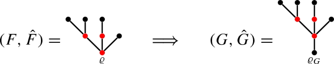
  The decorations of , as well as $\hat{G}$, coincide with those of $\tau$, except on the newly added edge/vertex where $\hat{G}$, $\bar{\mathfrak {n}}$ and $\bar{\mathfrak {o}}$ vanish, while $\bar{\mathfrak {e}}(\varrho _G,\varrho ) = k$. This gives a triangular operator and is therefore well defined.

• 3. Similarly, we define operators

  

  (4.13)

  in exactly the same way as the operators defined in (4.12), except that the root of is coloured with the colour 2, for instance

  

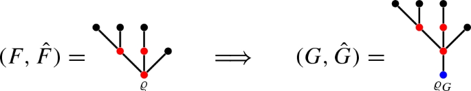
• 4. For $\alpha \in \mathbf{Z}^d\oplus \mathbf{Z}(\mathfrak {L})$, we define linear triangular maps in such a way that if $\tau = (T,\hat{T})_\mathfrak {e}^{\mathfrak {n},\mathfrak {o}}\in H_\circ$ with root $\varrho \in N_T$, then coincides with $\tau$, except for $\mathfrak {o}(\varrho )$ to which we add $\alpha$ and $\hat{T}(\varrho )$ which is set to 1. In particular, one has .

Remark 4.16

With these notations, it follows from the definition of the sets $H_\circ$, $H_1$ and $\hat{H}_2$ that they can be constructed as follows.

• Every element of $H_\circ \setminus \{\mathbf {1}\}$ can be obtained from elements of the type $X^k$ by successive applications of the maps , , and the tree product (4.8).

• Every element of $H_1$ is the forest product of a finite number of elements of $H_\circ$.

• Every element of $\hat{H}_2$ is of the form

  

  (4.14)

  for some finite collection of elements $\tau _i \in H_\circ \setminus \{\mathbf {1}\}$, $\mathfrak {t}_i \in \mathfrak {L}$ and $k_i \in \mathbf{N}^d$.

Then, one obtains a simple recursive description of the coproduct $\Delta _2$.

Proposition 4.17

With the above notations, the operator is multiplicative, satisfies the identities

(4.15)

and it is completely determined by these properties. Likewise, is multiplicative, satisfies the identities on the first line of (4.15) and

(4.16)

and it is completely determined by these properties.

Proof

The operator $\Delta _2$ is multiplicative on as a consequence of the first identity of Proposition 4.10 and its action on $X^k$ was already mentioned in (3.43). It remains to verify that the recursive identities hold as well.

We first consider $\Delta _2 \sigma$ with and $\tau = (T,\hat{T})^{\mathfrak {n},\mathfrak {o}}_\mathfrak {e}$. We write $\sigma = (F,\hat{F})^{\mathfrak {n},\mathfrak {o}}_{\mathfrak {e}+ k \mathbf {1}_e}$, where e is the “trunk” of type $\mathfrak {t}$ created by and $\varrho$ is the root of F; moreover we extend $\mathfrak {n}$ to $N_F$ and $\mathfrak {o}$ to $N_{\hat{F}}$ by setting $\mathfrak {n}(\varrho )=\mathfrak {o}(\varrho )=0$. It follows from the definitions that

$$\begin{aligned} \mathfrak {A}_2(F,\hat{F}) = \{\{\varrho \}\} \cup \{ A \cup \{\varrho ,e\}\,:\, A \in \mathfrak {A}_2(T,\hat{T})\}\;. \end{aligned}$$

Indeed, if e does not belong to an element A of $\mathfrak {A}_2(F,\hat{F})$ then, since A has to contain $\varrho$ and be connected, one necessarily has $A = \{\varrho \}$. If on the other hand $e \in A$, then one also has $\varrho \in A$ and the remainder of A is necessarily a connected subtree of T containing its root, namely an element of $\mathfrak {A}_2(T,\hat{T})$.

Given $A \in \mathfrak {A}_2(T, \hat{T})$, since the root-label of $\sigma$ is 0, the set of all possible node-labels $\mathfrak {n}_A$ for $\sigma$ appearing in (3.7) for $\Delta _2 \sigma$ coincides with those appearing in the expression for $\Delta _2 \tau$, so that we have the identity

This is because $\mathfrak {n}(\varrho ) =0$, so that the sum over $\mathfrak {n}_{\varrho }$ contains only the zero term. Since , we are implicitly applying the appropriate contraction , see (4.6)–(4.9).

We now consider $\Delta _2 \sigma$ with . In this case, we write $\tau = (T,\hat{T})^{\mathfrak {n},\mathfrak {o}}_\mathfrak {e}$ so that, denoting by $\varrho$ the root of T, one has . We claim that in this case one has

This is non-trivial only in the case $\hat{T}(\varrho ) = 0$. In this case however, it is necessarily the case that $\hat{T}(e) = 0$ for every edge e incident to the root. This in turn guarantees that the family $\mathfrak {A}_2(T,\hat{T})$ remains unchanged by the operation of colouring the root. This implies that one has

This appears slightly different from the desired identity, but the latter then follows by observing that, for every , one has as elements of , thanks to the fact that we quotiented by the kernel of which sets the value of $\mathfrak {o}$ to 0 on the root. $\square$

We finally have the following results on the antipode of :

Proposition 4.18

Let be the antipode of . Then

• The algebra morphism is defined uniquely by the fact that and for all with

  

  (4.17)

  where denotes the (tree) product.

• On , one has the identity

  

  (4.18)

Proof

By (4.14) and by induction over the number of edges in $\tau$, this uniquely determines a morphism of , so it only remains to show that

The formula is true for $\tau = X^k$, so that, since both sides are multiplicative, it is enough to consider elements of the form for some . Exploiting the identity (4.17), one then has

as required.

A similar proof by induction yields (4.18): see the proof of Lemma 6.5 for an analogous argument. Note that (4.18) is also a direct consequence of Proposition 3.27 and more precisely of the fact that the bialgebras and are in cointeraction, as follows from Remark 3.28: see [25, Prop. 2] for a proof. Having this property, the antipode is a morphism of the -comodule . $\square$

In this section we have shown several useful recursive formulae that characterize $\Delta _2$, see also Sect. 6.4 below. The paper [4] explores in greater detail this recursive approach to Regularity Structures, and includes a recursive formula for $\Delta _1$, which is however more complex than that for $\Delta _2$.

5 Rules and associated regularity structures

We recall the definition of a regularity structure from [32, Def. 2.1]

Definition 5.1

A regularity structure$\mathscr {T}= (A, T, G)$ consists of the following elements:

• An index set $A \subset \mathbf{R}$ such that A is bounded from below, and A is locally finite.

• A model spaceT, which is a graded vector space $T = \bigoplus _{\alpha \in A} T_\alpha$, with each $T_\alpha$ a Banach space.

• A structure groupG of linear operators acting on T such that, for every $\Gamma \in G$, every $\alpha \in A$, and every $a \in T_\alpha$, one has

  $$\begin{aligned} \Gamma a - a \in \bigoplus _{\beta < \alpha } T_\beta \;. \end{aligned}$$

  (5.1)

The aim of this section is to relate the construction of the previous section to the theory of regularity structures as exposed in [32, 34]. For this, we first assign real-valued degrees to each element of $\mathfrak {F}$.

Definition 5.2

A scaling is a map $\mathfrak {s}:\{1,\ldots d\} \rightarrow [1,\infty )$ and a degree assignment is a map $|\cdot |_\mathfrak {s}:\mathfrak {L}\rightarrow \mathbf{R}\setminus \{0\}$. By additivity, we then assign a degree to each $(k,v) \in \mathbf{Z}^d\oplus \mathbf{Z}(\mathfrak {L})$ by setting

$$\begin{aligned} |(k,v)|_\mathfrak {s}{\mathop {=}\limits ^{ \text{ def }}}|k|_\mathfrak {s}+|v|_\mathfrak {s}\in \mathbf{R}, \qquad |k|_\mathfrak {s}{\mathop {=}\limits ^{ \text{ def }}}\sum _{i=1}^d k_i \mathfrak {s}_i , \qquad |v|_\mathfrak {s}{\mathop {=}\limits ^{ \text{ def }}}\sum _{\mathfrak {t}\in \mathfrak {L}} v_\mathfrak {t}\,|\mathfrak {t}|_\mathfrak {s}, \end{aligned}$$

(5.2)

if $v=\sum _{\mathfrak {t}\in \mathfrak {L}} v_\mathfrak {t}\mathfrak {t}$ with $v_\mathfrak {t}\in \mathbf{Z}$.

Definition 5.3

Given a scaling $\mathfrak {s}$ as above, for $\tau = (F,\hat{F}, \mathfrak {n},\mathfrak {o},\mathfrak {e}) \in \mathfrak {F}_2$, we define two different notions of degree $|\tau |_-, |\tau |_+ \in \mathbf{R}$ by

$$\begin{aligned} |\tau |_-&= \sum _{e \in E_F \setminus \hat{E}} \bigl (|\mathfrak {t}(e)|_{\mathfrak {s}} - |\mathfrak {e}(e)|_\mathfrak {s}\bigr ) + \sum _{x \in N_F} |\mathfrak {n}(x)|_\mathfrak {s}\;,\\ |\tau |_+&= \sum _{e \in E_F\setminus {\hat{E}_2}} \bigl (|\mathfrak {t}(e)|_{\mathfrak {s}} - |\mathfrak {e}(e)|_\mathfrak {s}\bigr ) + \sum _{x \in N_F} |\mathfrak {n}(x)|_\mathfrak {s}+ \sum _{x \in N_F \setminus {\hat{N}_2}} |\mathfrak {o}(x)|_\mathfrak {s}\;, \end{aligned}$$

where we recall that $\mathfrak {o}$ takes values in $\mathbf{Z}^d\oplus \mathbf{Z}(\mathfrak {L})$ and $\mathfrak {t}:E_F\rightarrow \mathfrak {L}$ is the map assigning to an edge its type in F, see Sect. 2.1.

Note that both of these degrees are compatible with the contraction operator of Definition 3.18, as well as the operator $\mathscr {J}$, in the sense that $|\tau |_\pm = |\bar{\tau }|_\pm$ if and only if and similarly for $\mathscr {J}$. In the case of $|\cdot |_+$, this is true thanks to the definition (3.33), while the coloured part of the tree is simply ignored by $|\cdot |_-$. We furthermore have

Lemma 5.4

The degree $|\cdot |_-$ is compatible with the operators and of (3.39), while $|\cdot |_+$ is compatible with and . Furthermore, both degrees are compatible with $\mathscr {J}$ and , so that in particular is $|\cdot |_-$-graded and and are both $|\cdot |_-$ and $|\cdot |_+$-graded.

Proof

The first statement is obvious since $|\cdot |_-$ ignores the coloured part of the tree, except for the labels $\mathfrak {n}$ whose total sum is preserved by all these operations. For the second statement, we need to verify that $|\cdot |_+$ is compatible with $\hat{\Phi }_2$ as defined just below (3.37). which is the case when acting on a tree with $\varrho \in \hat{F}_2$ since the $\mathfrak {o}$-decoration of nodes in $\hat{F}_2$ does not contribute to the definition of $|\cdot |_+$. $\square$

As a consequence, $|\cdot |_-$ yields a grading for , $|\cdot |_+$ yields a grading for , and both of them yield gradings for . With these definitions, we see that we obtain a structure resembling a regularity structure by taking to be our model space, with grading given by $|\cdot |_+$ and structure group given by the character group of acting on via

$$\begin{aligned} \Gamma _g :{\langle \mathfrak {F}_\circ \rangle } \rightarrow {\langle \mathfrak {F}_\circ \rangle }\;,\quad \Gamma _g \tau = (\mathrm {id}\otimes g) \Delta _2 \tau \;. \end{aligned}$$

The second statement of Proposition 4.14 then guarantees that this action is multiplicative with respect to the tree product (4.8) on , so that we are in the context of [32, Sec. 4]. There are however two conditions that are not met:

• 1. The action of on is not of the form “identity plus terms of strictly lower degree”, as required for regularity structures.

• 2. The possible degrees appearing in have no lower bound and might have accumulation points.

We will fix the first problem by encoding in our context what we mean by considering a “subcritical problem”. Such problems will allow us to prune our structure in a natural way so that we are left with a subspace of that has the required properties. The second problem will then be addressed by quotienting a suitable subspace of by the terms of negative degree. The group of characters of the resulting Hopf algebra will then turn out to act on in the desired way.

5.1 Trees generated by rules

From now to Sect. 5.4 included, the colourings and the labels $\mathfrak {o}$ will be ignored. It is therefore convenient to consider the space

$$\begin{aligned} \mathfrak {T}{\mathop {=}\limits ^{ \text{ def }}}\{(T,\hat{T},\mathfrak {n},\mathfrak {o},\mathfrak {e})\in \mathfrak {F}: \, T \ \text {is a tree}, \ \hat{T}\equiv 0, \ \mathfrak {o}\equiv 0\}. \end{aligned}$$

(5.3)

In order to lighten notations, we write elements of $\mathfrak {T}$ as $(T,\mathfrak {n},\mathfrak {e}) = T_\mathfrak {e}^{\mathfrak {n}}$ with T a typed tree (for some set of types $\mathfrak {L}$) and $\mathfrak {n}:N_T \rightarrow \mathbf{N}^d$, $\mathfrak {e}:E_T \rightarrow \mathbf{N}^d$ as above. Similarly to before, $\mathfrak {T}$ is a monoid for the tree product (4.8). Again, this product is associative and commutative, with unit $(\bullet ,0,0)$.

Definition 5.5

We say that an element $T_\mathfrak {e}^{\mathfrak {n}}\in \mathfrak {T}$ is trivial if T consists of a single node $\bullet$. It is planted if T has exactly one edge incident to its root $\varrho$ and furthermore $\mathfrak {n}(\varrho ) = 0$.

In other words, a planted $T_\mathfrak {e}^{\mathfrak {n}}\in \mathfrak {T}$ is necessarily of the form with $\tau \in \mathfrak {T}$, see (4.12). For example,

With this definition, each $\tau \in \mathfrak {T}$ has by (4.14) a unique (up to permutations) factorisation with respect to the tree product (4.8)

$$\begin{aligned} \tau = \bullet _n \tau _1 \tau _2\ldots \tau _k\;, \end{aligned}$$

(5.4)

for some $n \in \mathbf{N}^d$, where each $\tau _i$ is planted and $\bullet _n$ denotes the trivial element $(\bullet ,n,0)\in \mathfrak {T}$.

In order to define a suitable substructure of the structure described in Proposition 4.14, we introduce the notion of “rules”. Essentially, a “rule” describes what behaviour we allow for a tree in the vicinity of any one of its nodes.

In order to formalise this, we first define the set of edge types and the set of node types by

(5.5)

where denotes the set of unordered-valued n-uples, namely , with the natural action of the symmetric group $S_n$ on . In other words, given any set A, consists of all finite multisets whose elements are elements of A.

Remark 5.6

The fact that we consider multisets and not just n-uples is a reflection of the fact that we always consider the situation where the tree product (4.8) is commutative. This condition could in principle be dropped, thus leading us to consider forests consisting of planar trees instead, but this would lead to additional complications and does not seem to bring any advantage.

Given two sets $A \subset B$, we have a natural inclusion . We will usually write elements of as n-uples with the understanding that this is just an arbitrary representative of an equivalence class. In particular, we write () for the unique element of .

Given any $T_\mathfrak {e}^{\mathfrak {n}} \in \mathfrak {T}$, we then associate to each node $x \in N_T$ a node type by

(5.6)

where $(e_1,\ldots ,e_n)$ denotes the collection of edges leaving x, i.e. edges of the form (x, y) for some node y. We will sometimes use set-theoretic notations. In particular, given and , we write

$$\begin{aligned} M \sqcup N {\mathop {=}\limits ^{ \text{ def }}}(r_1,\ldots ,r_\ell ,s_1,\ldots , s_n)\;, \end{aligned}$$

and we say that $M \subset N$ if there exists $\bar{N}$ such that $N = M \sqcup \bar{N}$. When we write a sum of the type $\sum _{M \subset N}$, we take multiplicities into account. For example (a, b) is contained twice in (a, b, b), so that such a sum always contains $2^{n}$ terms if N is an n-tuple. Similarly, we write $t \in N$ if $(t) \subset N$ and we also count sums of the type $\sum _{t \in N}$ with the corresponding multiplicities.

Definition 5.7

Denoting by the powerset of , a rule is a map . A rule is said to be normal if, whenever $M \subset N \in R(\mathfrak {t})$, one also has $M \in R(\mathfrak {t})$.

For example we may have $\mathfrak {L}=\{\mathfrak {t}_1,\mathfrak {t}_2\}$ and

Then, according to the rule R, an edge of type $\mathfrak {t}_1$ or $\mathfrak {t}_2$ can be followed in a tree by, respectively, no edge, or a single edge of type $\mathfrak {t}_i$ with decoration $\mathfrak {e}_i$ with $i\in \{1,2\}$, or by two edges, one of type $\mathfrak {t}_1$ with decoration $\mathfrak {e}_1$ and one of type $\mathfrak {t}_2$ with decoration $\mathfrak {e}_2$. We do not expect however to find two edges both of type $\mathfrak {t}_1$ (or $\mathfrak {t}_2$) sharing a node which is not the root.

Definition 5.8

Let R be a rule and $\tau = T_\mathfrak {e}^{\mathfrak {n}} \in \mathfrak {T}$. We say that

• $\tau$conforms toR at the vertex x if either x is the root and there exists $\mathfrak {t}\in \mathfrak {L}$ such that or one has , where e is the unique edge linking x to its parent in T.

• $\tau$conforms to R if it conforms to R at every vertex x, except possibly its root.

• $\tau$strongly conforms to R if it conforms to R at every vertex x.

In particular, the trivial tree $\bullet$ strongly conforms to every normal rule since, as a consequence of Definition 5.7, there exists at least one $\mathfrak {t}\in \mathfrak {L}$ with $() \in R(\mathfrak {t})$.

Example 5.9

Consider R as in (5.7) and the trees

The first tree does not conform to the rule R since the bottom left edge of type $\mathfrak {t}_2$ is followed by three edges. The second tree conforms to R but not strongly, since the root is incident to three edges. The third tree strongly conforms to R. If we call $\varrho _i$ the root of the i-th tree, then we have , , , see (5.6). Finally, note that R is normal.

Remark 5.10

If R is a normal rule, then by Definition 5.7 we have in particular that $()\in R(\mathfrak {t})$ for every $\mathfrak {t}\in \mathfrak {L}$. This guarantees that $\mathfrak {L}$ contains no useless labels in the sense that, for every $\mathfrak {t}\in \mathfrak {L}$, there exists a tree conforming to R containing an edge of type $\mathfrak {t}$: it suffices to consider a rooted tree with a single edge $e=(x,y)$ of type $\mathfrak {t}$; in this case, . More importantly, this also guarantees that we can build any tree conforming to R from the root upwards (start with an edge of type $\mathfrak {t}$, add to it a node of some type in $R(\mathfrak {t})$, then restart the construction for each of the outgoing edges of that node) in finitely many steps.

Remark 5.11

A rule R can be represented by a directed bipartite multigraph as follows. Take as the vertex set . Then, connect to if $t \in N$. If t is contained in N multiple times, repeat the connection the corresponding number of times. Conversely, connect to if $N \in R(\mathfrak {t})$. The conditions then guarantee that can be reached from every vertex in the graph. Given a tree $\tau \in \mathfrak {T}$, every edge of $\tau$ corresponds to an element of and every node corresponds to an element of via the map defined above. A tree then conforms to R if, for every path joining the root to one of the leaves, the corresponding path in V always follows directed edges in . It strongly conforms to R if the root corresponds to a vertex in V with at least one incoming edge.

Definition 5.12

Given $\mathfrak {s}$ as in Definition 5.2, we assign a degree $|\tau |_\mathfrak {s}$ to any $\tau \in \mathfrak {T}$ by setting

$$\begin{aligned} |T_\mathfrak {e}^\mathfrak {n}|_\mathfrak {s}= \sum _{e \in E_T} \bigl (|\mathfrak {t}(e)|_{\mathfrak {s}} - |\mathfrak {e}(e)|_\mathfrak {s}\bigr ) + \sum _{x \in N_T} |\mathfrak {n}(x)|_\mathfrak {s}\;. \end{aligned}$$

(5.8)

This definition is compatible with both notions of degree given in Definition 5.3, since we view $\mathfrak {T}$ as a subset of $\mathfrak {F}$ with $\hat{F}$ and $\mathfrak {o}$ identically 0. This also allows us to give the following definition.

Definition 5.13

Given a rule R, we write

• $\mathfrak {T}_\circ (R) \subset \mathfrak {T}$ for the set of trees that strongly conform to R

• $\mathfrak {T}_1(R) \subset \mathfrak {F}$ for the submonoid of $\mathfrak {F}$ (for the forest product) generated by $\mathfrak {T}_\circ (R)$

• $\mathfrak {T}_2(R) \subset \mathfrak {T}$ for the set of trees that conform to R.

Moreover, we write $\mathfrak {T}_-(R) \subset \mathfrak {T}_\circ (R)$ for the set of trees $\tau = T_\mathfrak {e}^\mathfrak {n}$ such that

• $|\tau |_\mathfrak {s}< 0$, $\mathfrak {n}(\varrho _\tau ) = 0$,

• if $\tau$ is planted, namely with $\bar{\tau }\in \mathfrak {T}$, see (4.12), then $|\mathfrak {t}|_\mathfrak {s}< 0$.

The second restriction on the definition of $\tau \in \mathfrak {T}_-(R)$ is related to the definition (5.22) of the Hopf algebra and of its characters group , that we call the renormalisation group and which plays a fundamental role in the theory, see e.g. Theorem 6.16.

5.2 Subcriticality

Given a map ${\mathrm {reg}}:\mathfrak {L}\rightarrow \mathbf{R}$ we will henceforth interpret it as maps and as follows: for and

$$\begin{aligned} {\mathrm {reg}}(\mathfrak {t},k) {\mathop {=}\limits ^{ \text{ def }}}{\mathrm {reg}}(\mathfrak {t})-|k|_\mathfrak {s}, \qquad {\mathrm {reg}}(N) {\mathop {=}\limits ^{ \text{ def }}}\sum _{(\mathfrak {t},k) \in N} {\mathrm {reg}}(\mathfrak {t},k), \end{aligned}$$

(5.9)

with the convention that the sum over the empty word is 0.

Definition 5.14

A rule R is subcritical with respect to a fixed scaling $\mathfrak {s}$ if there exists a map ${\mathrm {reg}}:\mathfrak {L}\rightarrow \mathbf{R}$ such that

$$\begin{aligned} {\mathrm {reg}}(\mathfrak {t}) < |\mathfrak {t}|_\mathfrak {s}+ \inf _{N \in R(\mathfrak {t})} {\mathrm {reg}}(N) \;, \qquad \forall \, \mathfrak {t}\in \mathfrak {L}, \end{aligned}$$

(5.10)

where we use the notation (5.9).

We will see in Sect. 5.4 below that classes of stochastic PDEs generate rules. In this context, the notion of subcriticality given here formalises the one given somewhat informally in [32]. In particular, we have the following result which is essentially a reformulation of [32, Lem. 8.10] in this context.

Proposition 5.15

If R is a subcritical rule, then, for every $\gamma \in \mathbf{R}$, the set $\{\tau \in \mathfrak {T}_\circ (R)\,:\, |\tau |_\mathfrak {s}\le \gamma \}$ is finite.

Proof

Fix $\gamma \in \mathbf{R}$ and let $T_\mathfrak {e}^\mathfrak {n}\in \mathfrak {T}_\circ (R)$ with $|T_\mathfrak {e}^\mathfrak {n}|_\mathfrak {s}\le \gamma$. Since there exists $c>0$ such that

$$\begin{aligned} |T_\mathfrak {e}^\mathfrak {n}|_\mathfrak {s}\ge |T_\mathfrak {e}^0|_\mathfrak {s}+ c|\mathfrak {n}| \end{aligned}$$

and there exist only finitely many trees in $\mathfrak {T}_\circ (R)$ of the type $|T_\mathfrak {e}^0|$ for a given number of edges, it suffices to show that the number $|E_T|$ of edges of T is bounded by some constant depending only on $\gamma$.

Since the set $\mathfrak {L}$ is finite, (5.10) implies that there exists a constant $\kappa > 0$ such that the bound

$$\begin{aligned} {\mathrm {reg}}(\mathfrak {t}) + \kappa \le |\mathfrak {t}|_\mathfrak {s}+ \inf _{N \in R(\mathfrak {t})}{\mathrm {reg}}(N)\;, \end{aligned}$$

(5.11)

holds for every $\mathfrak {t}\in \mathfrak {L}$ with the notation (5.9). We claim that for every planted $T_\mathfrak {e}^\mathfrak {n}\in \mathfrak {T}_\circ (R)$ such that the edge type of its trunk $e=(\varrho ,x)$ is , we have

$$\begin{aligned} {\mathrm {reg}}(\mathfrak {t},k)\le |T_\mathfrak {e}^\mathfrak {n}|_\mathfrak {s}- \kappa |E_T|. \end{aligned}$$

(5.12)

We denote the space of such planted trees by $\mathfrak {T}^{(\mathfrak {t},k)}_\circ (R)$. We verify (5.12) by induction on the number of edges $|E_T|$ of T. If $|E_T|=1$, namely the unique element of $E_T$ is the trunk $e=(\varrho ,x)$, then in the notation of (5.6) and by (5.11)

$$\begin{aligned} {\mathrm {reg}}(\mathfrak {t}) + \kappa \le |\mathfrak {t}|_\mathfrak {s}\quad \Longrightarrow \quad {\mathrm {reg}}(\mathfrak {t},k)\le |\mathfrak {t}|_\mathfrak {s}-|k|_\mathfrak {s}- \kappa \le |T_\mathfrak {e}^\mathfrak {n}|_\mathfrak {s}- \kappa . \end{aligned}$$

For a planted $T_\mathfrak {e}^\mathfrak {n}\in \mathfrak {T}_\circ (R)$ with $|E_T|>1$, then and by (5.11) and the induction hypothesis

$$\begin{aligned} {\mathrm {reg}}(\mathfrak {t})-|k|_\mathfrak {s}+ \kappa&\le |\mathfrak {t}|_\mathfrak {s}-|k|_\mathfrak {s}+ \sum _{i=1}^n \left[ {\mathrm {reg}}(\mathfrak {t}_i)-|k_i|_\mathfrak {s}\right] \\&\le |T_\mathfrak {e}^\mathfrak {n}|_\mathfrak {s}-\kappa (|E_T|-1) \;, \end{aligned}$$

where $s(e_i)=(\mathfrak {t}_i,k_i)$. Therefore (5.12) is proved for planted trees.

Given an arbitrary tree $T_\mathfrak {e}^\mathfrak {n}$ of degree at most $\gamma$ strongly conforming to the rule R, there exists $\mathfrak {t}_0\in \mathfrak {L}$ such that . We can therefore consider the planted tree $\bar{T}_\mathfrak {e}^\mathfrak {n}$ containing a trunk of type $\mathfrak {t}_0$ connected to the root of T, and with vanishing labels on the root and trunk respectively. It then follows that

$$\begin{aligned} \kappa |E_T| < \kappa |E_{\bar{T}}|&\le |\bar{T}_\mathfrak {e}^\mathfrak {n}|_\mathfrak {s}-{\mathrm {reg}}(\mathfrak {t}_0) = |T_\mathfrak {e}^\mathfrak {n}|_\mathfrak {s}+ |\mathfrak {t}_0|_\mathfrak {s}-{\mathrm {reg}}(\mathfrak {t}_0)\\&\le \gamma + \inf _{\mathfrak {t}\in \mathfrak {L}} \bigl (|\mathfrak {t}|_\mathfrak {s}-{\mathrm {reg}}(\mathfrak {t})\bigr )\;, \end{aligned}$$

and the latter expression is finite since $\mathfrak {L}$ is finite. The claim follows at once. $\square$

Remark 5.16

The inequality (5.10) encodes the fact that we would like to be able to assign a regularity ${\mathrm {reg}}(\mathfrak {t})$ to each component $u_{\mathfrak {t}}$ of our SPDE in such a way that the “naïve regularity” of the corresponding right hand side obtained by a power-counting argument is strictly better than ${\mathrm {reg}}(\mathfrak {t}) - |\mathfrak {t}|$. Indeed, $\inf _{N \in R(\mathfrak {t})} {\mathrm {reg}}(N)$ is precisely the regularity one would like to assign to $F_{\mathfrak {t}}(u,\nabla u,\xi )$. Note that if the inequality in (5.10) is not strict, then the conclusion of Proposition 5.15 may fail to hold.

Remark 5.17

Assuming that there exists a map ${\mathrm {reg}}$ satisfying (5.11) for a given $\kappa > 0$, one can find a map ${\mathrm {reg}}_\kappa$ that is optimal in the sense that it saturates the bound (5.12):

$$\begin{aligned} {\mathrm {reg}}_\kappa (\mathfrak {t},k) = \min _{T_\mathfrak {e}^\mathfrak {n}\in \mathfrak {T}^{(\mathfrak {t},k)}_\circ (R) } \left( |T_\mathfrak {e}^\mathfrak {n}|_\mathfrak {s}- \kappa |E_T| \right) \end{aligned}$$

where . We proceed as follows. Set ${\mathrm {reg}}_\kappa ^0(\mathfrak {t}) = +\infty$ for every $\mathfrak {t}\in \mathfrak {L}$ and then define recursively

$$\begin{aligned} {\mathrm {reg}}_\kappa ^{n+1}(\mathfrak {t}) = |\mathfrak {t}|_\mathfrak {s}- \kappa + \inf _{N \in R(\mathfrak {t})} {\mathrm {reg}}_\kappa ^n(N)\;. \end{aligned}$$

(5.13)

By recurrence we show that $n\mapsto {\mathrm {reg}}_\kappa ^n(\mathfrak {t})$ is decreasing and ${\mathrm {reg}}\le {\mathrm {reg}}_\kappa ^n$; then the limit

$$\begin{aligned} {\mathrm {reg}}_\kappa (\mathfrak {t}) = \lim _{n \rightarrow \infty } {\mathrm {reg}}_\kappa ^n(\mathfrak {t}) \end{aligned}$$

exists and has the required properties. If we extend ${\mathrm {reg}}_\kappa ^n$ to $N$ by (5.9), the iteration (5.13) can be interpreted as a min-plus network on the graph with arrows reversed, see Remark 5.11.

5.3 Completeness

Given an arbitrary rule (subcritical or not), there is no reason in general to expect that the actions of the analogues of the groups and constructed in Sect. 4 leave the linear span of $\mathfrak {T}_\circ (R)$ invariant. We now introduce a notion of completeness, which will guarantee later on that the actions of and do indeed leave the span of $\mathfrak {T}_\circ (R)$ (or rather an extension of it involving again labels $\mathfrak {o}$ on nodes) invariant. This eventually allows us to build, for large classes of subcritical stochastic PDEs, regularity structures allowing to formulate them, endowed with a large enough group of automorphisms to perform the renormalisation procedures required to give them canonical meaning.

Definition 5.18

Given and $m \in \mathbf{N}^d$, we define as the set of all n-tuples of the form $((\mathfrak {t}_1,k_1+m_1),\ldots ,(\mathfrak {t}_n,k_n+m_n))$ where the $m_i\in \mathbf{N}^d$ are such that $\sum _i m_i = m$.

Furthermore, we introduce the following substitution operation on . Assume that we are given , $M \subset N$ and an element which has the same size as M. In other words, if $M = (r_1,\ldots ,r_\ell )$, one has $\tilde{M} = (\tilde{M}_1,\ldots ,\tilde{M}_\ell )$ with . Then, writing $N = M \sqcup \bar{N}$, we define

(5.14)

Definition 5.19

Given a rule R, for any tree $T_\mathfrak {e}^\mathfrak {n}\in \mathfrak {T}_\circ (R)$ we associate to each edge $e\in E_T$ a set in the following recursive way. If $e = (x,y)$ and y is a leaf, namely the node-type of the vertex y is equal to the empty word , then we set

Otherwise, writing $(e_1,\ldots ,e_\ell )$ the incoming edges of y, namely $e_i=(y,v_i)$, we define

Finally, we define for every node $y\in N_T$ a set by if y is a leaf, and

if $(e_1,\ldots ,e_\ell )$ are the outgoing edges of y.

It is easy to see that, if we explore the tree from the leaves down, this specifies and uniquely for all edges and nodes of T.

Definition 5.20

A rule R is $\ominus$-complete with respect to a fixed scaling $\mathfrak {s}$ if, whenever $\tau \in \mathfrak {T}_-(R)$ and $\mathfrak {t}\in \mathfrak {L}$ are such that there exists $N \in R(\mathfrak {t})$ with , one also has

for every and for every multiindex m with $|m|_\mathfrak {s}+ |\tau |_\mathfrak {s}< 0$.

At first sight, the notion of $\ominus$-completeness might seem rather tedious to verify and potentially quite restrictive. Our next result shows that this is fortunately not the case, at least when we are in the subcritical situation.

Proposition 5.21

Let R be a normal subcritical rule. Then, there exists a normal subcritical rule $\bar{R}$ which is $\ominus$-complete and extends R in the sense that $R(\mathfrak {t}) \subset \bar{R}(\mathfrak {t})$ for every $\mathfrak {t}\in \mathfrak {L}$.

Proof

Given a normal subcritical rule R, we define a new rule by setting

(5.15)

where $R_-(\mathfrak {t};\tau )$ is the union of all collections of node types of the type

for some $N \in R(\mathfrak {t})$ with , some , and some multiindex m with $|m|_\mathfrak {s}+ |\tau |_\mathfrak {s}\le 0$. Since and $\mathfrak {T}_-(R)$ is finite by Proposition 5.15, this is again a valid rule. Furthermore, by definition, a rule R is $\ominus$-complete if and only if .

We claim that the desired rule $\bar{R}$ can be obtained by setting

It is straightforward to verify that $\bar{R}$ is $\ominus$-complete. (This follows from the fact that the sequence of rules is increasing and is closed under increasing limits.)

It remains to show that $\bar{R}$ is again normal and subcritical. To show normality, we note that if R is normal, then is again normal. This is because, by Definition 5.19, the sets used to build also have the property that if and $M \subset N$, then one also has . As a consequence, is normal for every n, from which the normality of $\bar{R}$ follows.

To show that $\bar{R}$ is subcritical, we first recall that by Remark 5.17, for $\kappa$ as in (5.11), we can find a maximal function ${\mathrm {reg}}_\kappa :\mathfrak {L}\rightarrow \mathbf{R}$ such that

$$\begin{aligned} {\mathrm {reg}}_\kappa (\mathfrak {t}) = |\mathfrak {t}|_\mathfrak {s}- \kappa + \inf _{N \in R(\mathfrak {t})} {\mathrm {reg}}_\kappa (N)\;. \end{aligned}$$

(5.16)

Furthermore, the extension of ${\mathrm {reg}}_\kappa$ to node types given by (5.9) is such that, for every node type N and every multiindex m, one has

$$\begin{aligned} {\mathrm {reg}}_\kappa (\partial ^m N)={\mathrm {reg}}_\kappa (N)- |m|_\mathfrak {s}\;. \end{aligned}$$

(5.17)

(We used a small abuse of notation here since $\partial ^m N$ is really a collection of node types. Since ${\mathrm {reg}}_\kappa$ takes the same value on each of them, this creates no ambiguity.)

We claim that the same function ${\mathrm {reg}}_\kappa$ also satisfies (5.10) for the larger rule . In view of (5.16) and of the definition (5.15) of , it is enough to prove that

$$\begin{aligned} {\mathrm {reg}}_\kappa (\mathfrak {t}) \le |\mathfrak {t}|_\mathfrak {s}- \kappa +{\mathrm {reg}}(N), \qquad \forall \, N\in \bigcup _{\tau \in \mathfrak {T}_-(R)} R_-(\mathfrak {t};\tau ). \end{aligned}$$

(5.18)

Arguing by induction as in the proof of (5.12), one can first show the following. Let $\sigma \in \mathfrak {T}_\circ (R)$ any every planted tree whose trunk e has edge type $(\mathfrak {t},k)$. Then one has the bound

(5.19)

Indeed, if e is the only edge of $\sigma$, then and by (5.16)

$$\begin{aligned} {\mathrm {reg}}_\kappa (\mathfrak {t},k)\le |\mathfrak {t}|_\mathfrak {s}-|k|_\mathfrak {s}+{\mathrm {reg}}_\kappa (G)=|\sigma |_\mathfrak {s}+{\mathrm {reg}}_\kappa (G). \end{aligned}$$

If now $e=(x,y)$ and $(e_1,\ldots ,e_\ell )$ are the outgoing edges of y, then is the set of all with and $M=(M_1,\ldots ,M_\ell )$ with . By the induction hypothesis,

where $\sigma _i$ is the largest planted subtree of $\sigma$ with trunk $e_i$. Then

Combining this with (5.16) we obtain, since $|\mathfrak {t}|_\mathfrak {s}- |k|_\mathfrak {s}+\sum _{i=1}^\ell |\sigma _i|_\mathfrak {s}=|\sigma |_\mathfrak {s}$,

and (5.19) is proved.

We prove now (5.18). Let $\tau \in \mathfrak {T}_-(R)$, $N \in R(\mathfrak {t})$ with , , and $m\in \mathbf{N}^d$ with $|m|_\mathfrak {s}+ |\tau |_\mathfrak {s}\le 0$. Let $\tau = \tau _1\ldots \tau _\ell$ be the decomposition of $\tau$ into planted trees. Recalling (5.17) and Definitions 5.19 and 5.18, we have

where $s_i$ is the edge type of the trunk of $\tau _i$. Combining this with (5.19) yields

with the last inequality a consequence of the condition $|m|_\mathfrak {s}+ |\tau |_\mathfrak {s}\le 0$. This proves (5.18).

We conclude that (5.16) also holds when considering , thus yielding the desired claim. Iterating this, we conclude that ${\mathrm {reg}}_\kappa$ satisfies (5.10) for each of the rules and therefore also for $\bar{R}$ as required. $\square$

Definition 5.22

We say that a subcritical rule R is complete (with respect to a fixed scaling $\mathfrak {s}$) if it is both normal and $\ominus$-complete. If R is only normal, we call the rule $\bar{R}$ constructed in the proof of Proposition 5.21 the completion of R.

5.4 Three prototypical examples

Let us now show how, concretely, a given stochastic PDE (or system thereof) gives rise to a rule in a natural way. Let us start with a very simple example, the KPZ equation formally given by

$$\begin{aligned} \partial _{t} u = \Delta u + \left( \partial _x u \right) ^{2} + \xi \;. \end{aligned}$$

One then chooses the set $\mathfrak {L}$ so that it has one element for each noise process and one for each convolution operator appearing in the equation. In this case, using the variation of constants formula, we rewrite the equation in integral form as

$$\begin{aligned} u = P u_0 + P * \mathbf {1}_{t > 0}\bigl (\left( \partial _x u \right) ^{2} + \xi \bigr )\;, \end{aligned}$$

where P denotes the heat kernel and $*$ is space–time convolution. We therefore need two types in $\mathfrak {L}$ in this case, which we call in order to be consistent with [32].

We assign degrees to these types just as in [32]. In our example, the underlying space–time dimension is $d=2$ and the equation is parabolic, so we fix the parabolic scaling $\mathfrak {s}= (2,1)$ and then assign to $\Xi$ a degree just below the exponent of self-similarity of white noise under the scaling $\mathfrak {s}$, namely $|\Xi |_\mathfrak {s}= -{3\over 2} - \kappa$ for some small $\kappa > 0$. We also assign to each type representing a convolution operator the degree corresponding to the amount by which it improves regularity in the sense of [32, Sec. 4]. In our case, this is given by .

It then seems natural to assign to such an equation a rule $\tilde{R}$ by

where is a shorthand for the edge type and we simply write $\mathfrak {t}$ as a shorthand for the edge type $(\mathfrak {t},0)$. In other words, for every noise type $\mathfrak {t}$, we set $\tilde{R}(\mathfrak {t}) = \{()\}$ and for every kernel type $\mathfrak {t}$ we include one node type into $\tilde{R}(\mathfrak {t})$ for each of the monomials in our equation that are convolved with the corresponding kernel. The problem is that such a rule is not normal. Therefore we define rather

which turns out to be normal and complete. It is simple to see that the function

makes R subcritical for sufficiently small $\kappa >0$.

One can also consider systems of equations. Consider for example the system of coupled KPZ equations formally given by

$$\begin{aligned} \partial _{t} u_1&= \Delta u_1 + \left( \partial _x u_1 \right) ^{2} + \xi _1\;, \\ \partial _{t} u_2&= \nu \Delta u_2 + \left( \partial _x u_2 \right) ^{2} + \Delta u_1 + \xi _2\;. \end{aligned}$$

In this case, we have two noise types $\Xi _{1,2}$ as well as two kernel types, which we call for the heat kernel with diffusion constant 1 and for the heat kernel with diffusion constant $\nu$. There is some ambiguity in this case whether the term $\Delta u_1$ appearing in the second equation should be considered part of the linearisation of the equation or part of the nonlinearity. In this case, it turns out to be more convenient to consider this term as part of the nonlinearity, and we will see that the corresponding rule is still subcritical thanks to the triangular structure of this system.

Using the same notations as above, the normal and complete rule R naturally associated with this system of equations is given by

In this case, we see that R is again subcritical for sufficiently small $\kappa >0$ with

Our last example is given by the following generalisation of the KPZ equation:

$$\begin{aligned} \partial _{t} u = \Delta u + g(u) \left( \partial _x u \right) ^2 + h(u) \partial _{x} u + k(u) + f(u) \xi \;, \end{aligned}$$

which is motivated by (1.6) above, see [33]. In this case, the set $\mathfrak {L}$ is again given by , just as in the case of the standard KPZ equation. Writing as a shorthand for where is repeated $\ell$ times, the rule R associated to this equation is given by

Again, it is straightforward to verify that R is subcritical and that one can use the same map ${\mathrm {reg}}_\kappa$ as in the case of the standard KPZ equation. Even though in this case there are infinitely many node types appearing in , this is not a problem because , so that repetitions of the symbol in a node type only increase the corresponding degree.

5.5 Regularity structures determined by rules

Throughout this section, we assume that we are given

• a finite type set $\mathfrak {L}$ together with a scaling $\mathfrak {s}$ and degrees $|\cdot |_\mathfrak {s}$ as in Definition 5.2,

• a normal rule R for $\mathfrak {L}$ which is both subcritical and complete, in the sense of Definition 5.22,

• the integer $d\ge 1$ which has been fixed at the beginning of the paper.

We show that the above choices, when combined with the structure built in Sects. 3 and 4, yield a natural substructure with the same algebraic properties (the only exception being that the subspace of we consider is not an algebra in general), but which is sufficiently small to yield a regularity structure. Furthermore, this regularity structure contains a very large group of automorphisms, unlike the slightly smaller structure described in [32]. The reason for this is the additional flexibility granted by the presence of the decoration $\mathfrak {o}$, which allows to keep track of the degrees of the subtrees contracted by the action of .

Definition 5.23

We define for every $\tau =(G,\mathfrak {n}',\mathfrak {e}')\in \mathfrak {T}$ and every node $x\in N_G$ a set $D(x,\tau ) \subset \mathbf{Z}^d \oplus \mathbf{Z}(\mathfrak {L})$ by postulating that $\alpha \in D(x,\tau )$ if there exist

• $\sigma =(F,\mathfrak {n},\mathfrak {e})\in \mathfrak {T}$

• $A\subset F$ is a subtree such that $\sigma$ conforms to the rule R at every node $y \in A$

• functions $\mathfrak {n}_A :N_A \rightarrow \mathbf{N}^d$ with $\mathfrak {n}_A\le \mathfrak {n}{\upharpoonright }N_A$ and $\varepsilon _A^F:\partial (A,F)\rightarrow \mathbf{N}^d$

such that $(A,0,\mathfrak {n}_A+\pi \varepsilon _A^F,0,\mathfrak {e})\in \mathfrak {T}_-(R)$ (see Definition 5.13) and

(5.20)

and in particular

$$\begin{aligned} \alpha =\sum _{N_A}\left( \mathfrak {n}_A + \pi (\varepsilon _A^F-\mathfrak {e}_\varnothing ^A)\right) . \end{aligned}$$

We define by .

Definition 5.24

We denote by $\Lambda =\Lambda (\mathfrak {L},R,\mathfrak {s},d)$ the set of all $\tau = (F,\hat{F}, \mathfrak {n},\mathfrak {o},\mathfrak {e})\in \mathfrak {F}$ such that and, for all $x\in N_F$, exactly one of the following two mutually exclusive statements holds.

• One has $\hat{F}(x) \in \{0,2\}$ and $\mathfrak {o}(x)=0$.

• One has $\hat{F}(x) = 1$ and .

Lemma 5.25

Let $\sigma = (F,\hat{F}, \mathfrak {n},\mathfrak {o},\mathfrak {e})\in \Lambda$ and $A \in \mathfrak {A}_1(F,\hat{F})$ be a subforest such that $\sigma$ conforms to the rule R at every vertex $x \in A$ and fix functions $\mathfrak {n}_A :N_A \rightarrow \mathbf{N}^d$ with $\mathfrak {n}_A\le \mathfrak {n}{\upharpoonright }N_A$ and $\varepsilon _A^F:\partial (A,F)\rightarrow \mathbf{N}^d$. Assume furthermore that for each connected component B of A, we have $(B,0,\mathfrak {n}_A+\pi \varepsilon _A^F,0,\mathfrak {e})\in \mathfrak {T}_-(R)$, see Definition 5.13. Then the element

(5.21)

also belongs to $\Lambda$.

Conversely, every element $\tau$ of $\Lambda$ is of the form (5.21) for an element $\sigma$ with $\hat{F}(x) \in \{0,2\}$ and $\mathfrak {o}\equiv 0$.

Proof

Let us start by showing the last assertion. Let $\tau =(G,\hat{G},\mathfrak {n}',\mathfrak {o}',\mathfrak {e}')\in \Lambda$ and $\{x_1,\ldots ,x_n\}\subset N_G$ all nodes is such that $\hat{G}(x_i)=1$. Let us argue by recurrence over $i\in \{1,\ldots ,n\}$. By Definition 5.23 one can write

as in (5.20). Setting $F=F_n$ and $A=A_n$ we have the required representation.

Now the first assertion follows easily from the second one. $\square$

We now define spaces of coloured forests $\tau = (F,\hat{F}, \mathfrak {n},\mathfrak {o},\mathfrak {e})$ such that $(F,0,\mathfrak {n},0,\mathfrak {e})$ is compatible with the rule R in a suitable sense, and such that $\tau \in \Lambda$.

Definition 5.26

Recalling Definition 5.13 and Remark 4.13, we define the bigraded spaces

Remark 5.27

The superscript “ex” stands for “extended”, see Sect. 6.4 below for an explanation of the reason why we choose this terminology. The identification of these spaces as suitable subspaces of , and is done via the canonical basis (4.10).

Note that both and are algebras for the products inherited from and respectively. On the other hand, is in general not an algebra anymore.

Lemma 5.28

We have

as well as for . Moreover, is a Hopf subalgebra of and is a right Hopf-comodule over with coaction $\Delta _2$.

Proof

By the normality of the rule R, if a tree conforms to R then any of its subtrees does too. On the other hand, contracting subforests can generate non-conforming trees in the case of $\Delta _1$, while, since $\Delta _2$ extracts only subtrees at the root, completeness of the rule implies that this can not happen in the case of $\Delta _2$, thus showing that the maps $\Delta _i$ do indeed behave as claimed.

The fact that is in fact a Hopf algebra, namely that the antipode of leaves invariant, can be shown by induction using (4.17) and Remark 4.16. $\square$

Note that is a sub-algebra but in general not a sub-coalgebra of (and a fortiori not a Hopf algebra). Recall also that, by Lemma 5.4, the grading $|\cdot |_-$ of Definition 5.3 is well defined on and on , and that $|\cdot |_+$ is well defined on both and . Furthermore, these gradings are preserved by the corresponding products and coproducts.

Definition 5.29

Let be the ideals given by

(5.22)

Then, we set

(5.23)

with canonical projections . Moreover, we define the operator as .

With these definitions at hand, it turns out that the map $(\mathfrak {p}_-^\mathrm {ex}\otimes \mathrm {id})\Delta _1$ is much better behaved. Indeed, we have the following.

Lemma 5.30

The map $\Delta ^{\!-}_\mathrm {ex}= (\mathfrak {p}_-^\mathrm {ex}\otimes \mathrm {id})\Delta _1$ satisfies

Proof

This follows immediately from Lemma 5.28, combined with the fact that completeness of R has beed defined in Definition 5.20 in terms of extraction of $\tau \in \mathfrak {T}_-(R)$, which in particular means that $|\tau |_\mathfrak {s}=|\tau |_-<0$. $\square$

Analogously to Lemma 3.21 we have

Lemma 5.31

We have

(5.24)

Proof

We note that the degrees $|\cdot |_\pm$ have the following compatibility properties with the operators $\Delta _i$. For $0<i\le j\le 2$, $\tau \in \mathfrak {F}_j$ and $\Delta _i\tau =\sum \tau ^{(1)}_i\otimes \tau ^{(2)}_i$ (with the summation variable suppressed), one has

$$\begin{aligned} |\tau ^{(1)}_1|_- +|\tau ^{(2)}_1|_-=|\tau |_-\;, \quad |\tau ^{(2)}_1|_+=|\tau |_+\;,\quad |\tau ^{(1)}_2|_+ +|\tau ^{(2)}_2|_+=|\tau |_+ \;. \end{aligned}$$

(5.25)

The first identity of (5.24) then follows from the first identity of (5.25) and from the following remark: if , then for each term appearing in the sum over $A\in \mathfrak {A}_1$ in the expression (3.7) for $\Delta _1\tau$, one has two possibilities:

• either A does not contain the edge incident to the root of $\tau$, and then the second factor is a tree with only one edge incident to its root,

• or A does contain the edge incident to the root, in which case the first factor contains one connected component of that type.

The second identity of (5.24) follows from the second identity of (5.25) combined with the fact that, for $\tau \in \mathfrak {F}_2$, $\Delta _1 \tau$ contains no term of the form $\sigma \otimes \mathbf {1}_2$, even when quotiented by . The third identity of (5.24) finally follows from the third identity of (5.25), combined with the fact that if $\tau \in B_+\setminus \{\mathbf {1}_2\}$ with $|\tau |_+\le 0$, then the term $\mathbf {1}_2 \otimes \mathbf {1}_2$ does not appear in the expansion for $\Delta _2 \tau$. $\square$

As a corollary, we have the following.

Corollary 5.32

The operator $\Delta ^{\!-}_\mathrm {ex}= (\mathfrak {p}_-^\mathrm {ex}\otimes \mathrm {id})\Delta _1$ is well-defined as a map

Similarly, the operator $\Delta ^{\!+}_\mathrm {ex}= (\mathrm {id}\otimes \mathfrak {p}_+^\mathrm {ex}) \Delta _2$ is well-defined as a map

Remark 5.33

The operators $\Delta _\mathrm {ex}^{\pm }$ of Corollary 5.32 are now given by finite sums so that for all of these choices of , the operators $\Delta ^{\!-}_\mathrm {ex}$ and $\Delta ^{\!+}_\mathrm {ex}$ actually map into and respectively.

Proposition 5.34

There exists an algebra morphism so that , where is the tree product (4.8), is a Hopf algebra. Moreover the map , turns into a right comodule for with counit $\mathbf {1}^\star _2$.

Proof

We already know that is a Hopf sub-algebra of with antipode satisfying (4.17). Since is a bialgebra ideal by Lemma 5.31, the first claim follows from [48, Thm 1.(iv)].

The fact that is a co-action and turns into a right comodule for follows from the coassociativity of $\Delta _2$. $\square$

Proposition 5.35

There exists an algebra morphism so that is a Hopf algebra. Moreover the map turns into a left comodule for with counit $\mathbf {1}^\star _1$.

Proof

One difference between and is that is not in general a sub-coalgebra of and therefore it does not possess an antipode. However we can see that the antipode of satisfies for all $\tau \ne \mathbf {1}$

where is the product map. By the second formula of (5.25), it follows that if $|\tau |_->0$ then and therefore, since is an algebra morphism, . We obtain that defines a unique algebra morphism which is an antipode for . $\square$

Definition 5.36

We call the character group of .

We have therefore obtained the following analogue of Proposition 4.14:

Theorem 5.37

• 1. On , we have the identity

  

  (5.26)

  holds, with as in (3.49). The same is also true on .

• 2. Let . We define a left action of on by

  

  and a right action of on by

  

  Then we have

  

  (5.27)

Proof

By the second identity of (5.25), the action of $\Delta ^{\!-}_{\mathrm {ex}}$ preserves the degree $|\cdot |_{+}$. In particular we have

$$\begin{aligned} \Delta ^{\!-}_{\mathrm {ex}} \mathfrak {p}_+^{\mathrm {ex}} = \left( \mathrm {id}\otimes \mathfrak {p}_{+}^{\mathrm {ex}} \right) \Delta ^{\!-}_{\mathrm {ex}}. \end{aligned}$$

(5.28)

From this property, one has:

and we conclude by applying the Proposition 3.27. Now the proof of (5.27) is the same as that of (4.11) above. $\square$

Formula (5.26) yields the cointeraction property see Remark 3.28.

Remark 5.38

We can finally see here the role played by the decoration $\mathfrak {o}$: were it not included, the cointeraction property (5.26) of Theorem 5.37 would fail, since it is based upon (5.28), which itself depends on the second identity of (5.25). Now recall that $|\cdot |_+$ takes the decoration $\mathfrak {o}$ into account, and this is what makes the second identity of (5.25) true. See also Remark 6.26 below.

As in the discussion following Proposition 4.14, we see that is a left comodule over the Hopf algebra , with coaction

where $\sigma ^{(132)}(a\otimes b\otimes c){\mathop {=}\limits ^{ \text{ def }}}a\otimes c\otimes b$ and is the antipode of .

We define $A^\mathrm {ex}{\mathop {=}\limits ^{ \text{ def }}}\{|\tau |_+:\tau \in B_\circ \}$, where as in Definition 5.26.

Proposition 5.39

The above construction yields a regularity structure in the sense of Definition 5.1.

Proof

By the definitions, every element $\tau \in B_\circ$ has a representation of the type (5.21) for some $\sigma = (T,0,\mathfrak {n},0,\mathfrak {e}) \in \mathfrak {T}$. Furthermore, it follows from the definitions of $|\cdot |_+$ and $|\cdot |_\mathfrak {s}$ that one has $|\tau |_+ = |\sigma |_\mathfrak {s}$. The fact that, for all $\gamma \in \mathbf{R}$, the set $\{a\in A^\mathrm {ex}: a\le \gamma \}$ is finite then follows from Proposition 5.15.

The space is graded by $|\cdot |_+$ and acts on it by $\Gamma _g{\mathop {=}\limits ^{ \text{ def }}}(\mathrm {id}\otimes g)\Delta ^{\!+}_\mathrm {ex}$. The property (5.1) then follows from the fact $\Delta ^{\!+}_\mathrm {ex}$ preserves the total $|\cdot |_+$-degree by the third identity in (5.25) and all terms appearing in the second factor of $\Delta ^{\!+}_\mathrm {ex}\tau - \tau \otimes \mathbf {1}$ have strictly positive $|\cdot |_+$-degree by Definition 5.29. $\square$

Remark 5.40

Since is finitely generated as an algebra (though infinite-dimensional as a vector space), its character group is a finite-dimensional Lie group. In contrast, is not finite-dimensional but can be given the structure of an infinite-dimensional Lie group, see [5].

6 Renormalisation of models

We now show how the construction of the previous sections can be applied to the theory of regularity structures to show that the “contraction” operations one would like to perform in order to renormalise models are “legitimate” in the sense that they give rise to automorphisms of the regularity structures built in Sect. 5.5. Throughout this section, we are in the framework set at the beginning of Sect. 5.5. We furthermore impose the additional constraint that, writing $\mathfrak {L}= \mathfrak {L}_- \sqcup \mathfrak {L}_+$ with $\mathfrak {t}\in \mathfrak {L}_+$ if and only if $|\mathfrak {t}|_\mathfrak {s}> 0$, one has

$$\begin{aligned} \mathfrak {t}\in \mathfrak {L}_- \quad \Rightarrow \quad R(\mathfrak {t}) = \{()\}\;. \end{aligned}$$

(6.1)

Remark 6.1

Labels in $\mathfrak {L}_+$ represent “kernels” while labels in $\mathfrak {L}_+$ represent “noises”, which naturally leads to (6.1). (We could actually have defined $\mathfrak {L}_-$ by $\mathfrak {L}_- = \{\mathfrak {t}\,:\, R(\mathfrak {t}) = \{()\}\}$.) The condition that elements of $\mathfrak {L}_-$ are of negative degree and those in $\mathfrak {L}_+$ are of positive degree is also natural in this context. It could in principle be weakened, which corresponds to allowing kernels with a non-integrable singularity at the origin. This would force us to slightly modify Definition 6.8 below in order to interpret these kernels as distributions but would not otherwise lead to any additional complications.

Note now that we have a natural identification of with the subspaces

Denote by the corresponding inclusions, so that we have direct sum decompositions

(6.2)

For instance, with this identification, the map defined in (4.13) associates to an element which can be viewed as if and only if its degree is positive, namely $|\tau |_+ + |\mathfrak {t}|_\mathfrak {s}- |k|_\mathfrak {s}> 0$.

Proposition 6.2

Let be the antipode of . Then

• is defined uniquely by the fact that and for all

  

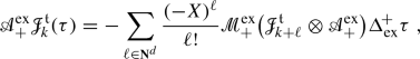  (6.3)

  where denotes the (tree) product and .

• On , one has the identity

  

  (6.4)

Proof

The claims follow easily from Propositions 4.18 and 5.34. $\square$

6.1 Twisted antipodes

We define now the operator given on $\tau \in B_+$ by

$$\begin{aligned} P_+(\tau ){\mathop {=}\limits ^{ \text{ def }}}\left\{ \begin{array}{ll} \tau \qquad &{} \text {if} |\tau |_+ > 0,\\ 0 &{} \text {otherwise.} \end{array}\right. \end{aligned}$$

Note that this is quite different from the projection $\mathfrak {i}_+^\mathrm {ex}\circ \mathfrak {p}_+^\mathrm {ex}$. However, for elements of the form for some , we have . The difference is that $\mathfrak {i}_+^\mathrm {ex}\circ \mathfrak {p}_+^\mathrm {ex}$ is multiplicative under the tree product, while $P_+$ is not.

Proposition 6.3

There exists a unique algebra morphism , which we call the “positive twisted antipode”, such that and furthermore for all

(6.5)

where is defined in (4.13), similarly to above is the product in and is as in Corollary 5.32.

Proof

Proceeding by induction over the number of edges appearing in $\tau$, one easily verifies that such a map exists and is uniquely determined by the above properties. $\square$

Comparing this to the recursion for given in (6.3), we see that they are very similar, but the projection $\mathfrak {p}_+^\mathrm {ex}$ in (6.3) is inside the multiplication , while $P_+$ in (6.5) is outside.

We recall now that the antipode is characterised among algebra-morphisms of by the identity

(6.6)

where is as in Corollary 5.32. The following result shows that satisfies a property close to (6.6), which is where the name “twisted antipode” comes from.

Proposition 6.4

The map satisfies the equation

(6.7)

where is as in Corollary 5.32.

Proof

Since both sides of (6.7) are multiplicative and since the identity obviously holds when applied to elements of the type $X^k$, we only need to verify that the left hand side vanishes when applied to elements of the form for some with $|\tau |_+ + |\mathfrak {t}|_\mathfrak {s}- |k|_\mathfrak {s}> 0$, and then use Remark 4.16. Similarly to the proof of (4.17), we have

since . $\square$

A very useful property of the positive twisted antipode is that its action is intertwined with that of $\Delta ^{\!-}_\mathrm {ex}$ in the following way.

Lemma 6.5

The identity

holds between linear maps from to .

Proof

Since both sides of the identity are multiplicative, by using Remark 4.16 it is enough to prove the result on $X_i$ and on elements of the form . The identity clearly holds on the linear span of $X^k$ since $\Delta ^{\!-}_\mathrm {ex}$ acts trivially on them and preserves that subspace.

Using the recursion (6.5) for , the identity $\Delta ^{\!-}_{\mathrm {ex}} P_+ =(\mathrm {id}\otimes P_+) \Delta ^{\!-}_{\mathrm {ex}}$ on , followed by the fact that $\Delta ^{\!-}_\mathrm {ex}$ is multiplicative, we obtain

Using the fact that , as well as (5.26), we have

Here, the passage from the penultimate to the last line crucially relies on the fact that the action of onto preserves the $|\cdot |_+$-degree, i.e. on the second formula in (5.25). $\square$

We have now a similar construction of a negative twisted antipode.

Proposition 6.6

There exists a unique algebra morphism , that we call the “negative twisted antipode”, such that for

(6.8)

Similarly to (6.7), the morphism satisfies

(6.9)

where is as in Corollary 5.32.

Proof

Proceeding by induction over the number of colourless edges appearing in $\tau$, one easily verifies that such a morphism exists and is uniquely determined by (6.8). The property (6.9) is a trivial consequence of (6.8). $\square$

6.2 Models

We now recall (a simplified version of) the definition of a model for a regularity structure given in [32, Def. 2.17]. Given a scaling $\mathfrak {s}$ as in Definition 5.2 and interpreting our constant $d\in \mathbf{N}$ as a space(-time) dimension, we define a metric $d_\mathfrak {s}$ on $\mathbf{R}^d$ by

$$\begin{aligned} \Vert x-y\Vert _\mathfrak {s}{\mathop {=}\limits ^{ \text{ def }}}\sum _{i=1}^d |x_i - y_i|^{1/\mathfrak {s}_i}\;. \end{aligned}$$

(6.10)

Note that $\Vert \cdot \Vert _\mathfrak {s}$ is not a norm since it is not 1-homogeneous, but it is still a distance function since $\mathfrak {s}_i \ge 1$. It is also homogeneous with respect to the (inhomogeneous) scaling in which the ith component is multiplied by $\lambda ^{\mathfrak {s}_i}$.

Definition 6.7

A smooth model for a given regularity structure $\mathscr {T}= (A,T,G)$ on $\mathbf{R}^d$ with scaling $\mathfrak {s}$ consists of the following elements:

• A map $\Gamma :\mathbf{R}^d\times \mathbf{R}^d \rightarrow G$ such that $\Gamma _{xx} = \mathrm {id}$, the identity operator, and such that $\Gamma _{xy}\, \Gamma _{yz} = \Gamma _{xz}$ for every x, y, z in $\mathbf{R}^d$.

• A collection of continuous linear maps such that $\Pi _y = \Pi _x \circ \Gamma _{xy}$ for every $x,y \in \mathbf{R}^d$.

Furthermore, for every $\ell \in A$ and every compact set $\mathfrak {K}\subset \mathbf{R}^d$, we assume the existence of a constant $C_{\ell ,\mathfrak {K}}$ such that the bounds

$$\begin{aligned} |\Pi _x \tau (y)| \le C_{\ell ,\mathfrak {K}} \Vert \tau \Vert _\ell \, \Vert x-y\Vert _\mathfrak {s}^\ell , \qquad \Vert \Gamma _{xy} \tau \Vert _m \le C_{\ell ,\mathfrak {K}} \Vert \tau \Vert _\ell \, \Vert x-y\Vert _\mathfrak {s}^{\ell -m}\;, \end{aligned}$$

(6.11)

hold uniformly over all $x,y \in \mathfrak {K}$, all $m\in A$ with $m < \ell$ and all $\tau \in T_\ell$.

Here, recalling that the space T in Definitions 5.1 and 6.7 is a direct sum of Banach spaces $(T_\alpha )_{\alpha \in A}$, the quantity $\Vert \sigma \Vert _m$ appearing in (6.11) denotes the norm of the component of $\sigma \in T$ in the Banach space $T_m$ for $m\in A$. We also note that Definition 6.7 does not include the general framework of [32, Def. 2.17], where $\Pi _x$ takes values in rather than ; however this simplified setting is sufficient for our purposes, at least for now. The condition (6.11) on $\Pi _x$ is of course relevant only for $\ell >0$ since $\Pi _x \tau (\cdot )$ is assumed to be a smooth function at this stage.

Recall that we fixed a label set $\mathfrak {L}= \mathfrak {L}_- \sqcup \mathfrak {L}_+$. We also fix a collection of kernels $\{K_{\mathfrak {t}}\}_{\mathfrak {t}\in \mathfrak {L}_+}$, $K_{\mathfrak {t}}:\mathbf{R}^d\setminus \{0\}\rightarrow \mathbf{R}$, satisfying the conditions of [32, Ass. 5.1] with $\beta = |\mathfrak {t}|_\mathfrak {s}$. We use extensively the notations of Sect. 4.3.

Definition 6.8

Given a linear map , we define for all $z,\bar{z}\in \mathbf{R}^d$

• a character by extending multiplicatively

  

  for $\mathfrak {t}\in \mathfrak {L}_+$ and setting for $\mathfrak {l}\in \mathfrak {L}_-$.

• a linear map and a character by

  

  (6.12)

  where is the positive twisted antipode defined in (6.5)

• a linear map and a character by

  

  (6.13)

Finally, we write for the map given by (6.12) and (6.13).

We do not want to consider arbitrary maps $\varvec{\Pi }$ as above, but we want them to behave in a “nice” way with respect to the natural operations we have on . We therefore introduce the following notion of admissibility. For this, we note that, as a consequence of (6.1), the only basis vectors of the type with $\mathfrak {t}\in \mathfrak {L}_-$ belonging to are those with $\tau = X^\ell$ for some $\ell \in \mathbf{N}^d$, so we give them a special name by setting and $\Xi ^\mathfrak {l}= \Xi _{0,0}^\mathfrak {l}$.

Definition 6.9

Given a linear map , we set $\xi _\mathfrak {l}{\mathop {=}\limits ^{ \text{ def }}}\varvec{\Pi }\Xi ^\mathfrak {l}$ for $\mathfrak {l}\in \mathfrak {L}_-$. We then say that $\varvec{\Pi }$ is admissible if it satisfies

(6.14)

for all , $k,\ell \in \mathbf{N}^d$, $\mathfrak {t}\in \mathfrak {L}_+$, $\mathfrak {l}\in \mathfrak {L}_-$, where is defined by (4.12), $*$ is the distributional convolution in $\mathbf{R}^d$, and we use the notation

$$\begin{aligned} D^k=\prod _{i=1}^d\frac{\partial ^{k_i}}{\partial y_i^{k_i}}, \qquad x^k:\mathbf{R}^d\rightarrow \mathbf{R}, \quad x^k(y){\mathop {=}\limits ^{ \text{ def }}}\prod _{i=1}^dy_i^{k_i}. \end{aligned}$$

Note that this definition guarantees that the identity always holds, whether $\mathfrak {t}$ is in $\mathfrak {L}_-$ or in $\mathfrak {L}_+$.

It is then simple to check that, with these definitions, $\Pi _z \Gamma _{\!z\bar{z}} = \Pi _{\bar{z}}$ and $(\Pi ,\Gamma )$ satisfies the algebraic requirements of Definition 6.7. However, $(\Pi ,\Gamma )$ does not necessarily satisfy the analytical bounds (6.11), although one has the following.

Lemma 6.10

If $\varvec{\Pi }$ is admissible then, for every with $\mathfrak {t}\in \mathfrak {L}_+$, we have

(6.15)

Proof

It follows immediately from (4.16) and the admissibility of $\varvec{\Pi }$ that is a polynomial of degree . On the other hand, it follows from (6.7) that and its derivatives up to the required order (because taking derivatives commutes with the action of the structure group) vanish at z, so there is no choice of what that polynomial is, thus yielding the second identity. The first identity then follows by comparing the second formula to (6.12). $\square$

Remark 6.11

Lemma 6.10 shows that the positive twisted antipode is intimately related to Taylor remainders, see Remark 3.7 and (6.12).

Lemma 6.10 shows that $(\Pi ,\Gamma )$ satisfies the analytical property (6.11) on planted trees of the form . However this is not necessarily the case for products of such trees, since neither $\varvec{\Pi }$ nor $\Pi _z$ are assumed to be multiplicative under the tree product (4.8). If, however, we also assume that $\varvec{\Pi }$ is multiplicative, then the map always produces a bona fide model.

Proposition 6.12

If is admissible and such that, for all with and all $\alpha \in \mathbf{Z}^d\oplus \mathbf{Z}(\mathfrak {L})$, we have

(6.16)

then is a model for $\mathscr {T}^{\mathrm {ex}}$.

Proof

The proof of the algebraic properties follows immediately from (6.13). Regarding the analytical bound (6.11) on $\Pi _z \sigma$, it immediately follows from Lemma 6.10 in the case when $\sigma$ is of the form . For products of such elements, it follows immediately from the multiplicative property of $\varvec{\Pi }$ combined with the multiplicativity of the action of $\Delta ^{\!+}_\mathrm {ex}$ on , which imply that

$$\begin{aligned} \Pi _x (\sigma \bar{\sigma }) = (\Pi _x \sigma )\cdot (\Pi _x \bar{\sigma })\;. \end{aligned}$$

Regarding vectors of the type , it follows immediately from the last identity in (4.15) combined with (6.16) that .

The proof of the second bound in (6.11) for $\Gamma _{xy}$ is virtually identical to the one given in [32, Prop. 8.27], combined with Lemma 6.10. Formally, the main difference comes from the change of basis (6.31) mentioned in Sect. 6.4, but this does not affect the relevant bounds since it does not mix basis vectors of different $|\cdot |_+$-degree. $\square$

Remark 6.13

If a map is admissible and furthermore satisfies (6.16), then it is uniquely determined by the functions $\xi _\mathfrak {l}{\mathop {=}\limits ^{ \text{ def }}}\varvec{\Pi }\Xi ^\mathfrak {l}$ for $\mathfrak {l}\in \mathfrak {L}_-$. In this case, we call $\varvec{\Pi }$ the canonical lift of the functions $\xi _\mathfrak {l}$.

6.3 Renormalised Models

We now use the structure built in this article to provide a large class of renormalisation procedures, which in particular includes those used in [32, 39, 42]. For this, we first need a topology on the space of all models for a given regularity structure. Given two smooth models $(\Pi ,\Gamma )$ and $(\bar{\Pi },\bar{\Gamma })$, for all $\ell \in A$ and $\mathfrak {K}\subset \mathbf{R}^d$ a compact set, we define the pseudo-metrics

$$\begin{aligned} |\!|\!|(\Pi ,\Gamma ) ; (\bar{\Pi },\bar{\Gamma })|\!|\!|_{\ell ;\mathfrak {K}} {\mathop {=}\limits ^{ \text{ def }}}\Vert \Pi - \bar{\Pi }\Vert _{\ell ;\mathfrak {K}} + \Vert \Gamma - \bar{\Gamma }\Vert _{\ell ;\mathfrak {K}}\;, \end{aligned}$$

(6.17)

where

Here, the set denotes the set of test functions with support in the centred ball of radius one and all derivatives up to oder $1 + |\inf A|$ bounded by 1. Given , $\varphi _x^\lambda :\mathbf{R}^d\rightarrow \mathbf{R}$ denotes the translated and rescaled function

$$\begin{aligned} \varphi _x^\lambda (y){\mathop {=}\limits ^{ \text{ def }}}\lambda ^{-(\mathfrak {s}_1+\cdots +\mathfrak {s}_d)}\, \varphi \Big ( \bigl ((y_i-x_i)\lambda ^{-\mathfrak {s}_i}\bigr )_{i=1}^d\Big ), \qquad y\in \mathbf{R}^d, \end{aligned}$$

for $x\in \mathbf{R}^d$ and $\lambda >0$ as in [32]. Finally, ${\langle \cdot ,\cdot \rangle }$ is the usual $L^2$ scalar product.

Definition 6.14

We denote by $\mathscr {M}^\mathrm {ex}_{\infty }$ the space of all smooth models of the form for some admissible linear map in the sense of Definition 6.9. We endow $\mathscr {M}^\mathrm {ex}_{\infty }$ with the system of pseudo-metrics $(|\!|\!|\cdot ; \cdot |\!|\!|_{\ell ;\mathfrak {K}})_{\ell ;\mathfrak {K}}$ and we denote by $\mathscr {M}^\mathrm {ex}_0$ the completion of this metric space.

We refer to [32, Def. 2.17] for the definition of the space $\mathscr {M}^\mathrm {ex}$ of models of a fixed regularity structure. With that definition, $\mathscr {M}^\mathrm {ex}_0$ is nothing but the closure of $\mathscr {M}^\mathrm {ex}_{\infty }$ in $\mathscr {M}^\mathrm {ex}$.

In many singular SPDEs, one is naturally led to a sequence of models which do not converge as $\varepsilon \rightarrow 0$. One would then like to be able to “tweak” this model in such a way that it remains an admissible model but has a chance of converging as $\varepsilon \rightarrow 0$. A natural way of “tweaking” $\varvec{\Pi }^{(\varepsilon )}$ is to compose it with some linear map . This naturally leads to the following question: what are the linear maps $M^{\mathrm {ex}}$ which are such that if is an admissible model, then is also a model? We then give the following definition.

Definition 6.15

A linear map is an admissible renormalisation procedure if

• for every admissible such that , $\varvec{\Pi }M$ is admissible and

• the map extends to a continuous map from $\mathscr {M}^\mathrm {ex}_0$ to $\mathscr {M}^\mathrm {ex}_0$.

We define a right action of onto , with , by $g \mapsto M^{\mathrm {ex}}_g$ with

(6.18)

The following Theorem is one of the main results of this article.

Theorem 6.16

For every , the map is an admissible renormalisation procedure. Moreover the renormalised model is described by:

$$\begin{aligned} \Pi _{z}^g = \Pi _z M^{\mathrm {ex}}_g, \quad \gamma ^{g}_{z \bar{z}} = \gamma _{z \bar{z}} M^{\mathrm {ex}}_{g}\;. \end{aligned}$$

(6.19)

Proof

Let us fix and an admissible linear map $\varvec{\Pi }$ such that is a model and set $\varvec{\Pi }^g {\mathop {=}\limits ^{ \text{ def }}}\varvec{\Pi }M^{\mathrm {ex}}_g$. We check first that $\varvec{\Pi }^g$ is admissible, namely that it satisfies (6.14). First, we note that, in the sum over A in (3.7) defining , we have two mutually excluding possibilities:

• 1. A is a subforest of $\tau$

• 2. A contains the edge of type $\mathfrak {t}$ added by the operator or the root of as an isolated node (which has however positive degree and is therefore killed by the projection $\mathfrak {p}^\mathrm {ex}_-$ in $\Delta ^{\!-}_\mathrm {ex}$).

When we apply $g\mathfrak {p}^\mathrm {ex}_-$ to the terms corresponding to case 2, the result is 0 since A contains one planted tree (with same root as that of ) and by the definition (5.22) of . Therefore we have

Therefore

Since $X^k$ has positive degree, with a similar computation we obtain

$$\begin{aligned} \varvec{\Pi }^gX^k\tau&= (g\otimes \varvec{\Pi })\Delta ^{\!-}_\mathrm {ex}X^k\tau = (g\otimes \varvec{\Pi }X^k)\Delta ^{\!-}_\mathrm {ex}\tau \\&=(g\otimes x^k\varvec{\Pi })\Delta ^{\!-}_\mathrm {ex}\tau = x^k\varvec{\Pi }^g\tau \end{aligned}$$

and this shows that $\varvec{\Pi }^g$ is admissible.

Now we verify that, writing $M^{\mathrm {ex}}_g$ as before and , we have

$$\begin{aligned} \gamma _{z\bar{z}}^g = (g \otimes \gamma _{z\bar{z}})\Delta ^{\!-}_{\mathrm {ex}}\;,\qquad \Pi _z^g = (g \otimes \Pi _z)\Delta ^{\!-}_{\mathrm {ex}}\;. \end{aligned}$$

To show this, one first uses (6.4) to show that $f_{z}^g = (g \otimes f_z)\Delta ^{\!-}_{\mathrm {ex}}$, where f and $f^g$ are defined from $\varvec{\Pi }$ and $\varvec{\Pi }^g$ as in (6.12). Indeed, one has

One then uses (5.26) on to show that the required identity (6.19) for $\Pi _z^g$ holds. Indeed, it follows that

$$\begin{aligned} \Pi _{z}^{g}&= \left( \varvec{\Pi }^{g} \otimes f^{g}_z \right) \Delta ^{\!+}_{\mathrm {ex}} = \left( g \otimes \varvec{\Pi }\otimes g \otimes f_z \right) \left( \Delta ^{\!-}_{\mathrm {ex}} \otimes \Delta ^{\!-}_{\mathrm {ex}} \right) \Delta ^{\!+}_{\mathrm {ex}}\nonumber \\&=\left( g\otimes \varvec{\Pi }\otimes f_z \right) \left( \mathrm {id}\otimes \Delta ^{\!+}_{\mathrm {ex}} \right) \Delta ^{\!-}_{\mathrm {ex}} = (g \otimes \Pi _z) \Delta ^{\!-}_{\mathrm {ex}}. \end{aligned}$$

(6.20)

In other words, we have applied (5.27) for $(g,f,h)=(g,f_z,\varvec{\Pi })$. Regarding $\gamma _{z \bar{z}}$, we have analogously

(6.21)

Note now that, at the level of the character $\gamma _{z\bar{z}}$, the bound (6.11) reads $|\gamma _{z\bar{z}}(\tau )| \le \Vert z-\bar{z}\Vert _\mathfrak {s}^{|\tau |_+}$ as a consequence of the fact that $\Delta ^{\!+}_\mathrm {ex}$ preserves the sum of the $|\cdot |_+$-degrees of each factor. On the other hand, for every character g of and any $\tau$ belonging to either $B_\circ$ or $B_+$ (see Definition 5.26), the element $(g\otimes \mathrm {id})\Delta ^{\!-}_\mathrm {ex}\tau$ is a linear combination of terms with the same$|\cdot |_+$-degree as $\tau$. As a consequence, it is immediate that if a given model $(\Pi ,\Gamma )$ satisfies the bounds (6.11), then the renormalised model $(\Pi ^g,\Gamma ^g)$ satisfies the same bounds, albeit with different constants, depending on g. We conclude that indeed for every admissible such that , $\varvec{\Pi }^g$ is admissible and .

The exact same argument also shows that if we extend the action of to all of $\mathscr {M}^\mathrm {ex}$ by (6.20) and (6.21), then this yields a continuous action, which in particular leaves $\mathscr {M}^\mathrm {ex}_0$ invariant as required by Definition 6.15. $\square$

Note now that the group $\mathbf{R}^d$ acts on admissible (in the sense of Definition 6.9) linear maps in two different ways. First, we have the natural action by translations $T_h$, $h \in \mathbf{R}^d$ given by

$$\begin{aligned} \bigl (T_h(\varvec{\Pi }) \tau \bigr )(z) {\mathop {=}\limits ^{ \text{ def }}}\bigl (\varvec{\Pi }\tau \bigr )(z-h)\;. \end{aligned}$$

However, $\mathbf{R}^d$ can also be viewed as a subgroup of by setting

(6.22)

This also acts on admissible linear maps by setting

$$\begin{aligned} \bigl (\tilde{T}_h(\varvec{\Pi }) \tau \bigr )(z) {\mathop {=}\limits ^{ \text{ def }}}\bigl ((\varvec{\Pi }\otimes g_h)\Delta ^{\!+}_\mathrm {ex}\tau \bigr )(z) \;. \end{aligned}$$

(6.23)

Note that if $\varvec{\Pi }$ is admissible, then one has $T_h(\varvec{\Pi }) X^k = \tilde{T}_h(\varvec{\Pi })X^k$ for every $k \in \mathbf{N}^d$ and every $h \in \mathbf{R}^d$.

Definition 6.17

We say that a random linear map is stationary if, for every (deterministic) element $h \in \mathbf{R}^d$, the random linear maps $T_h(\varvec{\Pi })$ and $\tilde{T}_h(\varvec{\Pi })$ are equal in law. We also assume that $\varvec{\Pi }$ and its derivatives, computed at 0 have moments of all orders.

By Definition 5.26 and Remark 4.16, can be identified canonically with the free algebra generated by $B_\circ$. We write

for the associated canonical injection.

Every random stationary map in the sense of Definition 6.17 then naturally determines a (deterministic) character $g^-(\varvec{\Pi })$ of by setting

$$\begin{aligned} g^-(\varvec{\Pi })(\iota _\circ \tau ) {\mathop {=}\limits ^{ \text{ def }}}\mathbf{E}\left( \varvec{\Pi }\tau \right) (0)\;, \end{aligned}$$

(6.24)

for $\tau \in B_\circ$, where the symbol $\mathbf{E}$ on the right hand side denotes expectation over the underlying probability space. This is extended multiplicatively to all of . Then we can define a renormalised map by

(6.25)

where is the negative twisted antipode defined in (6.8) and satisfying (6.9).

Let us also denote by $B_{\circ }^-$ the (finite!) set of basis vectors $\tau \in B_\circ$ such that $|\tau |_- < 0$. The specific choice of used to define is very natural and canonical in the following sense.

Theorem 6.18

Let be stationary and admissible such that is a model in $\mathscr {M}^\mathrm {ex}_\infty$. Then, among all random functions of the form

with $M^{\mathrm {ex}}_g$ as in (6.18), is the only one such that, for all $h \in \mathbf{R}^d$, we have

(6.26)

We call the BPHZ renormalisation of $\varvec{\Pi }$.

Proof

We first show that does indeed have the desired property. We first consider $h = 0$ and we write for the map (not to be confused with $\Pi _0$)

$$\begin{aligned} \varvec{\Pi }_0 \tau = \mathbf{E}(\varvec{\Pi }\tau )(0)\;. \end{aligned}$$

Let us denote by $B_\circ ^\sharp$ the set of $\tau \in B_\circ ^{-}$ which are not of the form with $|\mathfrak {t}|_\mathfrak {s}>0$. The main point now is that, thanks to the definitions of $g^-(\varvec{\Pi })$ and $\Delta ^{\!-}_\mathrm {ex}$, we have the identity

Combining this with (6.25), we obtain for all $\tau \in B_\circ ^\sharp$

by the defining property (6.9) of the negative twisted antipode, since $\iota _\circ \tau$ belongs both to the image of $\mathfrak {i}_-^\mathrm {ex}$ and to the kernel of $\mathbf {1}^\star _{1}$.

Let now $\tau \in B_\circ ^-$ be of the form with $|\mathfrak {t}|_\mathfrak {s}>0$, i.e. $\tau \in B_\circ ^-\setminus B_\circ ^\sharp$. Arguing as in the proof of Theorem 6.16 we see that

It then follows that

The definition of $g^-(\varvec{\Pi })$ combined with the fact that $\varvec{\Pi }$ is admissible and the definition of now implies that

where $D^k K_\mathfrak {t}$ should be interpreted in the sense of distributions. In particular, one has

(6.27)

For $\sigma = (F,\hat{F}, \mathfrak {n},\mathfrak {o},\mathfrak {e})$ and $\bar{\mathfrak {n}} :N_F \rightarrow \mathbf{N}^d$ with $\bar{\mathfrak {n}} \le \mathfrak {n}$, we now write $L_{\bar{\mathfrak {n}}}\sigma = (F,\hat{F}, \mathfrak {n}-\bar{\mathfrak {n}},\mathfrak {o},\mathfrak {e})$ and we note that for $g_h$ as in (6.22) one has the identity

$$\begin{aligned} (\mathrm {id}\otimes g_h)\Delta ^{\!+}_\mathrm {ex}\sigma = \sum _{\bar{\mathfrak {n}}} \left( {\begin{array}{c}\mathfrak {n}\\ \bar{\mathfrak {n}}\end{array}}\right) (-h)^{\Sigma \bar{\mathfrak {n}}} L_{\bar{\mathfrak {n}}}\sigma \;, \end{aligned}$$

so that the stationarity of $\varvec{\Pi }$ implies that

Plugging this into (6.27), we conclude that the terms for which there exists i with $k_i > (\Sigma \bar{\mathfrak {n}})_i$ vanish. If on the other hand one has $k_i \le (\Sigma \bar{\mathfrak {n}})_i$ for every i, then $|k|_\mathfrak {s}\le |\Sigma \bar{\mathfrak {n}}|_\mathfrak {s}$ and one has

so that $L_{\bar{\mathfrak {n}}}\sigma \in B_\circ ^-$ and has strictly less colourless edges than . If $\sigma$ has only one colourless edge, then $\sigma$ belongs to $B_\circ ^\sharp$; therefore the proof follows by induction over the number of colourless edges of $\tau$.

Let us now turn to the case $h \ne 0$. First, we claim that, setting , one has

(6.28)

This follows from the fact that $\hat{\varvec{\Pi }}$ is stationary since the action $\tilde{T}$ commutes with that of as a consequence of (5.26), combined with the fact that $(f \otimes g_h) \Delta ^{\!-}_\mathrm {ex}\tau = g_h(\tau )$ for every , every and every $g_h$ of the form (6.22).

On the other hand, we have

It follows immediately from the expression for the action of $\tilde{T}$ that is a deterministic linear combination of terms of the form with $|\sigma |_- \le |\tau |_-$, so that the claim (6.26) follows from (6.28).

It remains to show that $\hat{\varvec{\Pi }}$ is the only function of the type $\varvec{\Pi }^g$ with this property. For this, note that every such function is also of the form for some different , so that we only need to show that for every element g different from the identity, there exists $\tau$ such that .

Using Definitions 5.26 and 5.29, Remark 4.16 and the identification (6.2), can be canonically identified with the free algebra generated by $B_\circ ^\sharp$. Therefore the character g is completely characterised by its evaluation on $B_\circ ^\sharp$ and it is the identity if and only if this evaluation vanishes identically. Fix now such a g different from the identity and let $\tau \in B_\circ ^\sharp$ be such that $g(\tau ) \ne 0$, and such that $g(\sigma ) = 0$ for all $\sigma \in B_\circ ^\sharp$ with the property that either $|\sigma |_- < |\tau |_-$ or $|\sigma |_- = |\tau |_-$, but $\sigma$ has strictly less colourless edges than $\tau$. Since $B_\circ ^\sharp$ is finite and g doesn’t vanish identically, such a $\tau$ exists.

We can then also view $\tau$ as an element of and we write

$$\begin{aligned} \Delta ^{\!-}_\mathrm {ex}\tau = \tau \otimes \mathbf {1}_1 + \sum _i \tau _i^{(1)} \otimes \tau _i^{(2)}\;, \end{aligned}$$

so that

(6.29)

Note now that $\Delta ^{\!-}_\mathrm {ex}$ preserves the $|\cdot |_-$-degree so that for each of the term in the sum it is either the case that $|\tau _i^{(1)}|_- < |\tau |_-$ or that $|\tau _i^{(2)}| \le 0$. In the former case, the corresponding term in (6.29) vanishes identically by the definition of $\tau$. In the latter case, its expectation vanishes at the origin if $|\tau _i^{(2)}| < 0$ by (6.26). If $|\tau _i^{(2)}| = 0$ then, since $\tau _i^{(2)}$ is not proportional to $\mathbf {1}_1$ (this is the first term which was taken out of the sum explicitly), $\tau _i^{(2)}$ must contain at least one colourless edge. Since $\Delta ^{\!-}_\mathrm {ex}$ also preserves the number of colourless edges, this implies that again $g(\tau _i^{(1)}) = 0$ by our construction of $\tau$. We conclude that one has indeed , as required. $\square$

Remark 6.19

The rigidity apparent in (6.26) suggests that for a large class of random admissible maps built from some stationary processes $\xi _\mathfrak {t}^{(\varepsilon )}$ by (6.14) and (6.16), the corresponding collection of models built from defined as in (6.25) should converge to a limiting model, provided that the $\xi _\mathfrak {t}^{(\varepsilon )}$ converge in a suitable sense as $\varepsilon \rightarrow 0$. This is indeed the case, as shown in the companion “analytical” article [9]. It is also possible to verify that the renormalisation procedures that were essentially “guessed” in [31, 32, 39, 42] are precisely of BPHZ type, see Sects. 6.4.1 and 6.4.3 below.

Remark 6.20

One immediate consequence of Theorem 6.18 is that, for any and any admissible $\varvec{\Pi }$, if we set $\varvec{\Pi }^g = (g \otimes \varvec{\Pi })\Delta ^{\!-}_\mathrm {ex}$ as in Theorem 6.16, then the BPHZ renormalisation of $\varvec{\Pi }^g$ is . In particular, the BPHZ renormalisation of the canonical lift of a collection of stationary processes $\{\xi _\mathfrak {l}\}_{\mathfrak {l}\in \mathfrak {L}_-}$ as in Remark 6.13 is identical to that of the centred collection $\{\tilde{\xi }_\mathfrak {l}\}_{\mathfrak {l}\in \mathfrak {L}_-}$ where $\tilde{\xi }_\mathfrak {l}= \xi _\mathfrak {l}- \mathbf{E}\xi _\mathfrak {l}(0)$.

Remark 6.21

Although the map selects a “canonical” representative in the class of functions of the form $\varvec{\Pi }^g$, this does not necessarily mean that every stochastic PDE in the class described by the underlying rule R can be renormalised in a canonical way. The reason is that the kernels $K_\mathfrak {t}$ are typically some truncated version of the heat kernel and not simply the heat kernel itself. Different choices of the kernels $K_\mathfrak {t}$ may then lead to different choices of the renormalisation constants for the corresponding SPDEs.

6.4 The reduced regularity structure

In this section we study the relation between the regularity structure $\mathscr {T}^\mathrm {ex}$ introduced in this paper and the one originally constructed in [32, Sec. 8].

Definition 6.22

Let us call an admissible map reduced if the second identity in (6.16) holds, namely for all and $\alpha \in \mathbf{Z}^d\oplus \mathbf{Z}(\mathfrak {L})$. We also define the idempotent map by

with $\mathfrak d_1:\mathbf{N}\rightarrow \mathbf{N}$, , and set .

For example

An admissible map is reduced if and only if for every . Moreover commutes with the maps , and $\mathscr {J}$, and preserves the $|\cdot |_-$-degree, so that it is in particular also well-defined on , , and . It does however not preserve the $|\cdot |_+$-degree so that it is not well-defined on ! Indeed, the $|\cdot |_+$-degree depends on the $\mathfrak {o}$ decoration, which is set to 0 by , see Definition 5.3.

Definition 6.23

Let and respectively be the subspaces of and given by

We also set , where is defined after (5.23).

The reason why we define in this slightly more convoluted way instead of setting it equal to is that although is well-defined on , it is not well-defined on since it does not preserve the $|\cdot |_+$-degree, as already mentioned above. Since is multiplicative, is a subalgebra of . We set

(6.30)

Looking at the recursive definition (6.3) of the antipode , it is clear that it also maps into itself, so that is a Hopf subalgebra of . Moreover $\Delta$ turns into a co-module over .

We can therefore define as the characters group of and introduce the action of on :

If we grade by $|\cdot |_+$ and we define where and as in Definition 5.26, then arguing as in the proof of Proposition 5.39, we see that the action of on satisfies (5.1). Therefore $\mathscr {T}$ is a regularity structure as in Definition 5.1.

We set now and ,

(6.31)

Suppose that $\{\mathfrak {t},\mathfrak {i}\}\subseteq \mathfrak {L}$ with $|\mathfrak {t}|_\mathfrak {s}>0$ and $|\mathfrak {i}|_\mathfrak {s}<0$. We set . Then we have by (4.15) and (4.16) for all

(6.32)

as well as

(6.33)

with the additional property that both maps are multiplicative with respect to the tree product.

We see therefore that the operators and are isomorphic to those defined in [32, Eq. (8.8)–(8.9)]. This shows that the regularity structure $\mathscr {T}$, associated to a subcritical complete rule R, is isomorphic to the regularity structure associated to a subcritical equation constructed in [32, Sec. 8], modulo a simple change of coordinates. Note that this change of coordinates is “harmless” as far as the link to the analytical part of [32] is concerned since it does not mix basis vectors of different degrees.

As explained in Remark 5.27, the superscript ‘$\mathrm {ex}$’ stands for extended: the reason is that the regularity structure $\mathscr {T}^\mathrm {ex}$ is an extension of $\mathscr {T}$ in the sense that $\mathscr {T}\subset \mathscr {T}^\mathrm {ex}$ with the inclusion interpreted as in [32, Sec. 2.1]. By contrast, we call $\mathscr {T}$ the reduced regularity structure.

By the definition of , the extended structure encodes more information since we keep track of the effect of the action of by storing the (negative) homogeneity of the contracted subtrees in the decoration $\mathfrak {o}$ and by colouring the corresponding nodes; both these details are lost when we apply and therefore in the reduced structure .

Note that if is such that is a model of $\mathscr {T}^\mathrm {ex}$, then the restriction of to $\mathscr {T}$ is automatically again a model. This is always the case, irrespective of whether $\varvec{\Pi }$ is reduced or not, since the action of leaves invariant. This allows to give the following definition.

Definition 6.24

We denote by $\mathscr {M}_{\infty }$ the space of all smooth models for $\mathscr {T}$, in the sense of Definition 6.7, obtained by restriction to of for some reduced admissible linear map . We endow $\mathscr {M}_{\infty }$ with the system of pseudo-metrics (6.17) and we denote by $\mathscr {M}_0$ the completion of this metric space.

Remark 6.25

The restriction that $\varvec{\Pi }$ be reduced may not seem very natural in view of the discussion preceding the definition. It follows however from Theorem 6.33 below that lifting this restriction makes no difference whatsoever since it implies in particular that every smooth admissible model on $\mathscr {T}$ is of the form for some reduced $\varvec{\Pi }$.

Remark 6.26

By restriction of to $\mathscr {T}$ for , we get a renormalised model which covers all the examples treated so far in singular SPDEs. It is however not clear a priori whether we really have an action of a suitable subgroup of onto $\mathscr {M}_{\infty }$ or $\mathscr {M}_0$. This is because the coaction of $\Delta ^{\!-}_\mathrm {ex}$ on and fails to leave the reduced sector invariant. If on the other hand we tweak this coaction by setting , then unfortunately $\Delta ^{\!+}$ and $\Delta ^{\!-}$ do not have the cointeraction property (3.48), which was crucial for our construction, see Remark 5.38. See Corollary 6.37 below for more on $\Delta ^{\!-}$.

Remark 6.27

In accordance with [32, Formula (8.20)], it follows from (6.15) and the binomial identity that, for all with

Remark 6.28

The negative twisted antipode of Proposition 6.6 satisfies the identity . This follows from the induction (6.8), the multiplicativity of , and the formula

(6.34)

where . Therefore, if a stationary admissible $\varvec{\Pi }$ is (almost surely) reduced, then the character $g^-(\varvec{\Pi })$ is also reduced in the sense that . Using again (6.34), it follows immediately that as given by (6.25) is again reduced, so that the class of reduced models is preserved by the BPHZ renormalisation procedure.

There turn out to be two natural subgroups of that are determined by their values on :

• We set . This is the most natural subgroup of since it contains the characters used for the definition of $\hat{\varvec{\Pi }}$ in (6.25), as soon as . The fact that is a subgroup follows from the property (6.34).

• We set where is the bialgebra ideal of generated by . Then one can identify with the group of characters of the Hopf algebra . It turns out that this is simply the polynomial Hopf algebra with generators , so that is abelian.

We then have the following result.

Theorem 6.29

There is a continuous action R of onto $\mathscr {M}_0$ with the property that, for every and every reduced and admissible with , one has .

Proof

We already know by Theorem 6.16 that acts continuously onto $\mathscr {M}_0^\mathrm {ex}$. Furthermore, by the definition of , it preserves the subset $\mathscr {M}_0^r\subset \mathscr {M}_0^\mathrm {ex}$ of reduced models, i.e. the closure in $\mathscr {M}_0^\mathrm {ex}$ of all models of the form for $\varvec{\Pi }$ admissible and reduced. Since $\mathscr {T}\subset \mathscr {T}^\mathrm {ex}$, we already mentioned that we have a natural projection $\pi ^\mathrm {ex}:\mathscr {M}_0^\mathrm {ex}\rightarrow \mathscr {M}_0$ given by restriction (so that ), and it is straightforward to see that $\pi ^\mathrm {ex}$ is injective on $\mathscr {M}_0^r$. It therefore suffices to show that there is a continuous map $\iota ^\mathrm {ex}:\mathscr {M}_0 \rightarrow \mathscr {M}_0^\mathrm {ex}$ which is a right inverse to $\pi ^\mathrm {ex}$, and this is the content of Theorem 6.33 below. $\square$

Remark 6.30

We’ll show in Sect. 6.4.3 below that the action of onto $\mathscr {M}_0$ is given by elements of the “renormalisation group” defined in [32, Sec. 8.3].

6.4.1 An example

We consider the example of the stochastic quantization given in dimension 3 by:

$$\begin{aligned} \partial _t u = \Delta u + u^{3} + \xi . \end{aligned}$$

This equation has been solved first in [32] with regularity structures and then in [7]. One tree needed for its resolution reveals the importance of the extended decoration. Using the symbolic notation, it is given by . Then we use the following representation:

where $e_i$ is the ith canonical basis element of $\mathbf{N}^d$ and a belongs to $\lbrace \alpha , \beta , \gamma \rbrace$ with , and . Then we have

with summation over i and j implied. In (...) , we omit terms of the form $\tau ^{(1)} \otimes \tau ^{(2)}$ where $\tau ^{(1)}$ may contain planted trees or where $\tau ^{(2)}$ has an edge of type finishing on a leaf. The planted trees will disappear by applying an element of and the others are put to zero through the evaluation of the smooth model $\varvec{\Pi }$ see [32, Ass. 5.4] where the kernels $\{K_{\mathfrak {t}}\}_{\mathfrak {t}\in \mathfrak {L}_+}$ are chosen such that they integrate polynomials to zero up to a certain fixed order. If is the character associated to the BPHZ renormalisation for a Gaussian driving noise with a covariance that is symmetric under spatial reflections, we obtain

where

and all other renormalisation constants vanish. Applying , we indeed recover the renormalisation map given in [32, Sec 9.2]. The main interest of the extended decorations is to shorten some Taylor expansions which allows us to get the co-interaction between the two renormalisations. In the computation below, we show the difference between a term having extended decoration and the same without:

6.4.2 Construction of extended models

In general if, for some sequence , converges to a limiting model in $\mathscr {M}_0^\mathrm {ex}$, it does not follow that the characters $g_+(\varvec{\Pi }^{(n)})$ of converge to a limiting character. However, we claim that the characters $f_x^{(n)}$ of given by (6.12) do converge, which is not so surprising since our definition of convergence implies that the characters $\gamma _{xy}^{(n)}$ of given by (6.13) do converge. More surprising is that the convergence of the characters $f_x^{(n)}$ follows already from a seemingly much weaker type of convergence. Writing for the space of distributions on $\mathbf{R}^d$, we have the following.

Proposition 6.31

Let be an admissible linear map with

and assume that there exist linear maps such that, with the notation of (6.17), $\Vert \Pi ^{(n)} - \Pi \Vert _{\ell ,\mathfrak {K}} \rightarrow 0$ for every $\ell \in \mathbf{R}$ and every compact set . Then, the characters $f_x^{(n)}$ defined as in (6.12) converge to a limit $f_x$. Furthermore, defining $\Gamma _{xy}$ by (6.13), one has and in $\mathscr {M}_0^\mathrm {ex}$.

Finally, one has such that $\Pi _x = (\varvec{\Pi }\otimes f_x)\Delta ^{\!+}_\mathrm {ex}$ and such that $\varvec{\Pi }^{(n)}\tau \rightarrow \varvec{\Pi }\tau$ in   for every .

Proof

The convergence of the $f_x^{(n)}$ follows immediately from the formula given in Lemma 6.10, combined with the convergence of the $\Pi _x^{(n)}$ and [32, Lem. 5.19]. The fact that $(\Pi ,\Gamma )$ satisfies the algebraic identities required for a model follows immediately from the fact that this is true for every n. The convergence of the $\Gamma _{xy}^{(n)}$ and the analytical bound on the limit then follow from [32, Sec. 5.1]. $\square$

Remark 6.32

This relies crucially on the fact that the maps $\varvec{\Pi }$ under consideration are admissible and that the kernels $K_\mathfrak {t}$ satisfy the assumptions of [32, Sec. 5]. If one considers different notions of admissibility, as is the case for example in [40], then the conclusion of Proposition 6.31 may fail.

For a linear we define by simply setting . Then we say that $\varvec{\Pi }$ is admissible if $\varvec{\Pi }^\mathrm {ex}$ is. We have the following crucial fact

Theorem 6.33

If is admissible and belongs to $\mathscr {M}_\infty$, then belongs to $\mathscr {M}_\infty ^\mathrm {ex}$. Furthermore, the map extends to a continuous map from $\mathscr {M}_0$ to $\mathscr {M}_0^\mathrm {ex}$.

Before proving this Theorem, we define a linear map such that

$$\begin{aligned} L \Xi _{k,\ell }^\mathfrak {l}= \Xi _{k,\ell }^\mathfrak {l}\otimes \mathbf {1}\;,\qquad L X^k = X^k\otimes \mathbf {1}\;, \end{aligned}$$

and then recursively

as well as

(6.35)

where is the tree product (4.8) on and is as in (6.31).

Moreover is the algebra morphism such that $L_+ X^k = X^k$ and for with

(6.36)

The reason for these definitions is that these map will provide the required injection $\mathscr {M}_0 \rightarrow \mathscr {M}_0^\mathrm {ex}$ by (6.38) below. Before we proceed to show this, we state the following preliminary identity.

Lemma 6.34

On

(6.37)

Proof

We prove (6.37) by recursion. Both maps in (6.37) agree on elements of the form $\Xi _{k,\ell }^\mathfrak {l}$ or $X^k$ and both maps are multiplicative for the tree product. Consider now a tree of the form and assume that (6.37) holds when applied to $\tau$. Then we have by (6.32)

On the other hand

Comparing both right hand sides and using the induction hypothesis, we conclude that (6.37) does indeed hold as claimed. $\square$

Proof of Theorem 6.33

Let be such that is a model of $\mathscr {T}$ and write . In accordance with (6.12) and (6.13), we set

so that one has

$$\begin{aligned} \Pi _z^\mathrm {ex}= \bigl (\varvec{\Pi }^\mathrm {ex}\otimes f_z^\mathrm {ex}\bigr )\Delta ^{\!+}_{\mathrm {ex}} \;, \qquad \Gamma _{\!z\bar{z}}^\mathrm {ex}= \left( \mathrm {id}\otimes \gamma _{\!z\bar{z}}^\mathrm {ex}\right) \Delta ^{\!+}_{\mathrm {ex}} \;. \end{aligned}$$

With the notations introduced in (6.30), the model is then given by

where and similarly for $\gamma _{z\bar{z}}$. Define and by

$$\begin{aligned} \hat{\Pi }_z {\mathop {=}\limits ^{ \text{ def }}}(\Pi _z\otimes f_z)L, \qquad \hat{f}_z{\mathop {=}\limits ^{ \text{ def }}}f_z L_+\;, \end{aligned}$$

(6.38)

where $L,L_+$ are defined in (6.35)–(6.36). We want to show that for all z. By the definitions

By (6.37)

We want now to show that $\hat{f}_z\equiv f^\mathrm {ex}_z$ on . By Remark 6.27, for with we have

Therefore, by the definitions of $\hat{f}_z$ and $L_+$, for all with

which is equal to by Lemma 6.10 and Remark 6.27. Since $\hat{f}_z$ and $f^\mathrm {ex}_z$ are multiplicative linear functionals on and they coincide on a set which generates as an algebra, we conclude that $\hat{f}_z\equiv f^\mathrm {ex}_z$ on and therefore that $\hat{\Pi }_z\equiv \Pi ^\mathrm {ex}_z$ on . Finally, we can prove by recurrence that for all and

with $|\tau ^{(1)}_i|_+ \ge |\tau |_+$ and $|\bar{\tau }^{(1)}_i|_+ \ge |\bar{\tau }|_+$. This implies the required analytical estimates for $(\Pi ^\mathrm {ex},\Gamma ^\mathrm {ex})$. $\square$

6.4.3 Renormalisation group of the reduced structure

In this section, we show that the action of the renormalisation group on $\mathscr {M}_0$ given by Theorem 6.29 is indeed given by elements of the “renormalisation group” ${\mathfrak R}$ as defined in [32, Sec. 8.3]. This shows in particular that the BPHZ renormalisation procedure given in Theorem 6.18 does always fit into the framework developed there.

We recall that, by [32, Lem. 8.43, Thm 8.44] and [40, Thm B.1], ${\mathfrak R}$ is the set of linear operators satisfying the following properties.

• One has and $MX^k \tau =X^k M \tau$ for all $\mathfrak {t}\in \mathfrak {L}_+$, $k\in \mathbf{N}^d$, and .

• Consider the (unique) linear operators and such that $\hat{M}$ is an algebra morphism, $\hat{M} X^k=X^k$ for all k, and such that, for every and every and $k \in \mathbf{N}^d$ with ,

  

  (6.39)
  

  (6.40)

  where is defined by (6.31). Then, for all , one can write $\Delta ^{\!M}\tau = \sum \tau ^{(1)}\otimes \tau ^{(2)}$ with $| \tau ^{(1)}|_+ \ge | \tau |_+$.

Remark 6.35

Despite what a cursory inspection may suggest, the condition (6.39) is not equivalent to the same expression with replaced by . This is because (6.39) will typically fail to hold when .

We recall that the group has beed defined after Remark 6.28.

Theorem 6.36

Given , define $M_g^\mathrm {ex}$ on and as in (6.18) and let be given by . Then $M_g \in \mathfrak {R}$, $g \mapsto M_g$ is a group homomorphism, and one has the identities

(6.41)

where the maps $L,L_+$ are given in (6.35)–(6.36).

Proof

In order to check (6.39), it suffices by (6.41) to use (6.36) and the fact that $M_g^\mathrm {ex}$ preserves the $|\cdot |_+$-degree. It remains to check (6.40). We have on that

where we have used the co-interaction property in the last line. It follows from (6.37) that these two terms are indeed equal. The triangularity of L and $M^{\mathrm {ex}}_g$, combined with (6.41), implies the triangularity of $\Delta ^{\!M_g}$.

The homomorphism property follows from (6.34) and the definition of since

as required. $\square$

Corollary 6.37

The space inherits from a Hopf algebra structure and its group of characters is isomorphic to . Furthermore, the map

turns into a left comodule for .

Proof

This follows immediately from (6.34), Theorem 6.36, the definition of , the fact that is an algebra morphism on , and the same argument as in the proof of Proposition 4.11. $\square$

By the Remarks 6.19 and 6.28, the renormalisation procedures of [31, 32, 39, 42] can be described in this framework.

Appendices

Appendix A: Spaces and canonical basis vectors

The following diagram summarises the relations between the main spaces appearing in this article.

The next diagram similarly shows the relations between various sets of trees/forests. The first four columns in this diagram show the canonical basis vectors for the spaces appearing in the first four columns of the previous diagram.

Appendix B: Symbolic index

Here, we collect some of the most used symbols of the article, together with their meaning and the page where they were first introduced.

Symbol	Meaning	Page
$|\cdot |_{\mathrm {bi}}$	Bigrading on coloured decorated forests	18
$|\cdot |_-$	Degree not taking into account the label $\mathfrak {o}$	58
$|\cdot |_+$	Degree taking into account the label $\mathfrak {o}$	58
$\mathfrak {A}_i$	Subforests appearing in the definition of $\Delta _i$	20
	Antipode of	37
	Antipode of	72
	Twisted antipode	76
	Antipode of	52
$B_\circ$	Elements of $H_\circ$ strongly conforming to the rule R	70
$B_\circ ^-$	Elements of $B_\circ$ of negative degree	84
$B_\circ ^\sharp$	Elements of $B_\circ ^-$ that are not planted	85
$B_-$	Elements of $H_1$ strongly conforming to the rule R	70
$B_+$	Elements of $\hat{H}_2$ conforming to the rule R	70
$\mathfrak {B}_i$	Hopf algebra of coloured forests	33
$\mathfrak {C}$	All coloured forests $(F,\hat{F})$	14
$\mathfrak {C}_i$	All coloured forests compatible with $\mathfrak {A}_i$	29
	All roots of colour in $\{0,i\}$	48
	All roots of colour i	48
$\Delta _i$	Coproduct on ${\langle \mathfrak {F}\rangle }$ turning the ${\langle \mathfrak {F}_i\rangle }$ into bialgebras	22
	Edge types given by	60
$f {\upharpoonright }A$	Restriction of the function f to the set A	19
$\mathfrak {F}$	All decorated forests $(F,\hat{F}, \mathfrak {n},\mathfrak {o},\mathfrak {e})$	15
$\mathfrak {F}_i$	All decorated forests compatible with $\mathfrak {A}_i$	29
$\mathfrak {F}_\circ$	Trees with colours in $\{0,1\}$	51
$\Phi _i$	Collapse of factors in $\mathfrak {M}_i$	35
$g^+_z(\varvec{\Pi })$	Character on defined by $\varvec{\Pi }$	79
$g^-_z(\varvec{\Pi })$	Character on defined by $\varvec{\Pi }$	84
	Characters of	38
	Character group of	73
	Characters of	52
	Algebra given by	51
	Hopf algebra	50
	Hopf algebra	36
$H_\circ$	Representative of given by	52
$\hat{H}_2$	Representative of given by	52
$H_i$	Representative of given by	36
$\mathfrak {i}_\pm ^\mathrm {ex}$	Canonical injection	75
	Kernel of	36
	Kernel of	36
	Abstract integration map in	54
$\mathscr {J}$	Joins the root of all trees together	48
	Abstract integration map	54
	Subspace of terms in with a factor of positive degree	71
	Subspace of terms in with a factor of negative degree	71

Symbol	Meaning	Page
	Contraction of coloured portions	34
	Defined by	35
	Defined by	35
|k|	Unscaled length of a multi-index k	18
$|k|_\mathfrak {s}$	Scaled length of a multi-index k	58
$\mathfrak {L}$	Set of all types	13
$\mathfrak {M}_i$	Elements of $\mathfrak {F}_i$ completely coloured with i	35
$\mathscr {M}$	Space of all models	82
$\mathscr {M}_0$	Closure of smooth models	82
$\mathscr {M}_\infty$	Space of all smooth models	82
	Node types given by	60
	Type of the node x	60
$\hat{P}_i$	Sets $\mathfrak {o}$-decoration to 0 on i-coloured roots	35
	Powerset of the set A	60
	Multisets with elements from the set A	60
$\mathfrak {p}_\pm ^\mathrm {ex}$	Canonical projection	71
$\varvec{\Pi }$	Linear map specifying a model	79
R	Rule determining a class of trees	60
	Operator adding $\alpha$ to $\mathfrak {o}$ at the root	54
$\mathfrak {s}$	Scaling of $\mathbf{R}^d$	58
$\mathfrak {T}$	Simple decorated trees	59
$\mathfrak {T}_\circ (R)$	Trees strongly conforming to the rule R	62
$\mathfrak {T}_1(R)$	Forests strongly conforming to the rule R	62
$\mathfrak {T}_2(R)$	Trees conforming to the rule R	62
$\mathfrak {T}_-(R)$	Trees strongly conforming to R of negative degree	62
	Subspace of determined by a rule R	70
	Subspace of determined by a rule R	70
	Subspace of determined by a rule R	70
	Quotient space	71
	Quotient space	71
$\mathfrak {U}_i$	Units of ${\langle \mathfrak {F}_i\rangle }$	29
${\langle V\rangle }$	Bigraded space generated from a bigraded set V	19
$X^k$	Shorthand for $(\bullet ,i)_0^{k,0}$ with $i \in \{0,2\}$ depending on context	54
$\Xi ^\mathfrak {l}$	Element representing the noise	79
$\Vert z\Vert _\mathfrak {s}$	Scaled distance	78
	Map turning $\varvec{\Pi }$ into a model	79

References

Albeverio, S., Röckner, M.: Stochastic differential equations in infinite dimensions: solutions via Dirichlet forms. Probab. Theory Relat. Fields 89(3), 347–386 (1991). https://doi.org/10.1007/BF01198791
Bruned, Y., Chandra, A., Chevyrev, I., Hairer, M.: Renormalising SPDEs in regularity structures (2017). arXiv:1711.10239
Bogoliubow, N.N., Parasiuk, O.S.: Über die Multiplikation der Kausalfunktionen in der Quantentheorie der Felder. Acta Math. 97, 227–266 (1957). https://doi.org/10.1007/BF02392399
Bruned, Y.: Recursive formulae in regularity structures. Stoch. Partial Differ. Equ. Anal. Comput. 6(4), 25–564 (2018). https://doi.org/10.1007/s40072-018-0115-z. arXiv:1710.10634
Bogfjellmo, G., Schmeding, A.: The geometry of characters of Hopf algebras. vol. 13 of Symposium. Springer (2018). arXiv:1704.01099. https://doi.org/10.1007/978-3-030-01593-0
Cartier, P.: A primer of Hopf algebras. In: Cartier, P., Moussa, P., Julia, B., Vanhove, P. (eds.) Frontiers in Number Theory, Physics, and Geometry. II, pp. 537–615. Springer, Berlin (2007). https://doi.org/10.1007/978-3-540-30308-4_12
Catellier, R., Chouk, K.: Paracontrolled distributions and the 3-dimensional stochastic quantization equation. Ann. Probab. 46(5), 2621–2679 (2018). https://doi.org/10.1214/17-AOP1235. arXiv:1310.6869
Calaque, D., Ebrahimi-Fard, K., Manchon, D.: Two interacting Hopf algebras of trees: a Hopf-algebraic approach to composition and substitution of B-series. Adv. Appl. Math. 47(2), 282–308 (2011). https://doi.org/10.1016/j.aam.2009.08.003. arXiv:0806.2238
Chandra, A., Hairer, M.: An analytic BPHZ theorem for Regularity Structures (2016). arXiv:1612.08138
Chen, K.-T.: Iterated integrals and exponential homomorphisms. Proc. Lond. Math. Soc. (3) 4, 502–512 (1954)
Chen, K.-T.: Integration of paths, geometric invariants and a generalized Baker–Hausdorff formula. Ann. Math. (2) 65, 163–178 (1957)
Chen, K.-T.: Integration of paths—a faithful representation of paths by non-commutative formal power series. Trans. Am. Math. Soc. 89, 395–407 (1958)
Chen, K.-T.: Algebras of iterated path integrals and fundamental groups. Trans. Am. Math. Soc. 156, 359–379 (1971)
Chartier, P., Hairer, E., Vilmart, G.: A substitution law for B-series vector fields. Research Report RR-5498, INRIA. https://hal.inria.fr/inria-00070509 (2005)
Chartier, P., Hairer, E., Vilmart, G.: Algebraic structures of B-series. Found. Comput. Math. 10(4), 407–427 (2010). https://doi.org/10.1007/s10208-010-9065-1
Connes, A., Kreimer, D.: Hopf algebras, renormalization and noncommutative geometry. Commun. Math. Phys. 199(1), 203–242 (1998). https://doi.org/10.1007/s002200050499. arXiv:hep-th/9808042
Connes, A., Kreimer, D.: Renormalization in quantum field theory and the Riemann-Hilbert problem. J. High Energy Phys. 1999(9), 1–8 (1999). https://doi.org/10.1088/1126-6708/1999/09/024. arXiv:hep-th/9909126
Connes, A., Kreimer, D.: Renormalization in quantum field theory and the Riemann–Hilbert problem I: the Hopf algebra structure of graphs and the main theorem. Commun. Math. Phys. 210, 249–73 (2000). https://doi.org/10.1007/s002200050779. arXiv:hep-th/9912092
Connes, A., Kreimer, D.: Renormalization in quantum field theory and the Riemann–Hilbert problem. II. The \(\beta \)-function, diffeomorphisms and the renormalization group. Commun. Math. Phys. 216(1), 215–241 (2001). https://doi.org/10.1007/PL00005547. arXiv:hep-th/0003188
Da Prato, G., Debussche, A.: Two-dimensional Navier–Stokes equations driven by a space–time white noise. J. Funct. Anal. 196(1), 180–210 (2002). https://doi.org/10.1006/jfan.2002.3919
Da Prato, G., Debussche, A.: Strong solutions to the stochastic quantization equations. Ann. Probab. 31(4), 1900–1916 (2003). https://doi.org/10.1214/aop/1068646370
Ebrahimi-Fard, K., Guo, L., Kreimer, D.: Spitzer’s identity and the algebraic Birkhoff decomposition in pQFT. J. Phys. A 37(45), 11037–11052 (2004). https://doi.org/10.1088/0305-4470/37/45/020. arXiv:hep-th/0407082
Friz, P.K.: A Course on Rough Paths. Universitext, p. xiv+251. Springer, Cham (2014). https://doi.org/10.1007/978-3-319-08332-2. (With an introduction to regularity structures)
Feldman, J., Magnen, J., Rivasseau, V., Sénéor, R.: Bounds on Renormalized Feynman graphs. Commun. Math. Phys. 100(1), 23–55 (1985). https://doi.org/10.1007/BF01212686
Foissy, L.: Commutative and non-commutative bialgebras of quasi-posets and applications to Ehrhart polynomials (2016). arXiv:1605.08310
Gubinelli, M., Imkeller, P., Perkowski, N.: Paracontrolled distributions and singular PDEs. Forum Math. Pi 3, e6–75 (2015). https://doi.org/10.1017/fmp.2015.2. arXiv:1210.2684
Gubinelli, M., Perkowski, N.: KPZ reloaded. Commun. Math. Phys. 349(1), 165–269 (2017). https://doi.org/10.1007/s00220-016-2788-3. arXiv:1508.03877
Gubinelli, M.: Controlling rough paths. J. Funct. Anal. 216(1), 86–140 (2004). https://doi.org/10.1016/j.jfa.2004.01.002
Gubinelli, M.: Ramification of rough paths. J. Differ. Equ. 248(4), 693–721 (2010). https://doi.org/10.1016/j.jde.2009.11.015
Guo, L.: Algebraic Birkhoff decomposition and its applications. In: Ji, L., Liu, K., Yau, S-T., Zheng, Z-J. (eds.) Automorphic forms and the Langlands program, vol. 9 of Advanced Lectures in Mathematics (ALM), pp. 277–319. International Press, Somerville, MA (2010). arXiv:0807.2266
Hairer, M.: Solving the KPZ equation. Ann. Math. (2) 178(2), 559–664 (2013). https://doi.org/10.4007/annals.2013.178.2.4. arXiv:1109.6811
Hairer, M.: A theory of regularity structures. Invent. Math. 198(2), 269–504 (2014). https://doi.org/10.1007/s00222-014-0505-4. arXiv:1303.5113
Hairer, M.: The motion of a random string. In: Proceedings of the XVIII ICMP, to appear (2016). arXiv:1605.02192
Hairer, M.: Regularity structures and the dynamical \(\Phi ^4_3\) model. Curr. Dev. Math. 2014, 1–50 (2016). arXiv:1508.05261
Hepp, K.: On the equivalence of additive and analytic renormalization. Commun. Math. Phys. 14, 67–69 (1969). https://doi.org/10.1007/BF01645456
Hairer, M., Labbé, C.: A simple construction of the continuum parabolic Anderson model on \({ R}^2\). Electron. Commun. Probab. 20(43), 11 (2015). https://doi.org/10.1214/ECP.v20-4038. arXiv:1501.00692
Hairer, M., Labbé, C.: Multiplicative stochastic heat equations on the whole space. J. Eur. Math. Soc. 20(4), 1005–1054 (2018). https://doi.org/10.4171/JEMS/781. arXiv:1504.07162
Hoshino, M.: KPZ equation with fractional derivatives of white noise. Stoch. Partial Differ. Equ. Anal. Comput. 4(4), 827–890 (2016). https://doi.org/10.1007/s40072-016-0078-x. arXiv:1602.04570
Hairer, M., Pardoux, É.: A Wong–Zakai theorem for stochastic PDEs. J. Math. Soc. Jpn. 67(4), 1551–1604 (2015). https://doi.org/10.2969/jmsj/06741551. arXiv:1409.3138
Hairer, M., Quastel, J.: A class of growth models rescaling to KPZ. Forum Math. Pi, to appear (2015). arXiv:1512.07845
Hairer, M., Shen, H.: The dynamical sine-Gordon model. Commun. Math. Phys. 341(3), 933–989 (2016). https://doi.org/10.1007/s00220-015-2525-3. arXiv:1303.5113
Hairer, M., Shen, H.: A central limit theorem for the KPZ equation. Ann. Probab. 45(6B), 4167–4221 (2017). https://doi.org/10.1214/16-AOP1162. arXiv:1507.01237
Jona-Lasinio, G., Mitter, P.K.: On the stochastic quantization of field theory. Commun. Math. Phys. 101(3), 409–436 (1985)
Kreimer, D.: On the Hopf algebra structure of perturbative quantum field theories. Adv. Theor. Math. Phys. 2(2), 303–334 (1998). https://doi.org/10.4310/ATMP.1998.v2.n2.a4. arXiv:q-alg/9707029
Kupiainen, A.: Renormalization group and stochastic PDEs. Ann. Henri Poincaré 17(3), 497–535 (2016). https://doi.org/10.1007/s00023-015-0408-y. arXiv:1410.3094
Lyons, T.J.: Differential equations driven by rough signals. Rev. Mat. Iberoam. 14(2), 215–310 (1998). https://doi.org/10.4171/RMI/240
Molnar, R.K.: Semi-direct products of Hopf algebras. J. Algebra 47(1), 29–51 (1977). https://doi.org/10.1016/0021-8693(77)90208-3
Nichols, W.D.: Quotients of Hopf algebras. Commun. Algebra 6(17), 1789–1800 (1978). https://doi.org/10.1080/00927877808822321
Schmitt, W.R.: Antipodes and incidence coalgebras. J. Combin. Theory Ser. A 46(2), 264–290 (1987). https://doi.org/10.1016/0097-3165(87)90006-9
Schmitt, W.R.: Incidence Hopf algebras. J. Pure Appl. Algebra 96(3), 299–330 (1994). https://doi.org/10.1016/0022-4049(94)90105-8
Shen, H., Xu, W.: Weak universality of dynamical \(\Phi ^4_3\): non-Gaussian noise. Stoch. Partial Differ. Equ. Anal. Comput. 6(2), 211–254 (2018). https://doi.org/10.1007/s40072-017-0107-4. arXiv:1601.05724
Zimmermann, W.: Convergence of Bogoliubov’s method of renormalization in momentum space. Commun. Math. Phys. 15, 208–234 (1969). https://doi.org/10.1007/BF01645676
Zhu, R., Zhu, X.: Three-dimensional Navier–Stokes equations driven by space-time white noise. J. Differ. Equ. 259(9), 4443–4508 (2015). https://doi.org/10.1016/j.jde.2015.06.002. arXiv:1406.0047
Acknowledgements
We are very grateful to Christian Brouder, Ajay Chandra, Alessandra Frabetti, Dominique Manchon and Kurusch Ebrahimi-Fard for many interesting discussions and pointers to the literature. MH gratefully acknowledges support by the Leverhulme Trust and by an ERC consolidator grant, project 615897 (Critical). LZ gratefully acknowledges support by the Institut Universitaire de France and the project of the Agence Nationale de la Recherche ANR-15-CE40-0020-01 grant LSD. The authors thank the organisers and the participants of a workshop held in Bergen in April 2017, where the results of this paper were presented and discussed in detail.
Author information
Authors and Affiliations
Corresponding author
Additional information
Publisher's Note
Springer Nature remains neutral with regard to jurisdictional claims in published maps and institutional affiliations.