A Scattering Theory for Linearised Gravity on the Exterior of the Schwarzschild Black Hole I: The Teukolsky Equations

Abstract

We construct a scattering theory for the spin $\pm \,2$ Teukolsky equations on the exterior of the Schwarzschild spacetime, as a first step towards developing a scattering theory for the linearised Einstein equations in double null gauge. This is done by exploiting a physical-space version of the Chandrasekhar transformation used by Dafermos et al. in (Acta Math 222(1):1–214, 2019. https://doi.org/10.4310/acta.2019.v222.n1.a1) to prove the linear stability of the Schwarzschild solution. We also address the Teukolsky–Starobinsky correspondence and construct an isomorphism between scattering data for the $+\,2$ and $-\,2$ Teukolsky equations. This will allow us to state an additional mixed scattering statement for a pair of curvature components satisfying the spin $+\,2$ and $-\,2$ Teukolsky equations and connected via the Teukolsky–Starobinsky identities, completely determining the radiating degrees of freedom of solutions to the linearised Einstein equations.

1 Introduction and Overview

Scattering theory has been an important tool in the mathematical and theoretical study of black hole solutions to the Einstein equations, which in vacuum take the form

$$\begin{aligned} R_{ab}[g]=0 \end{aligned}$$

(1.1)

(setting the cosmological constant to zero). Whereas there has been extensive work on scattering for scalar, electromagnetic, fermionic fields on black hole backgrounds (see already [7, 21, 23, 24, 39]), in the case of the scattering of gravitational perturbations much of the historic literature has been concerned with solutions to equations governing fixed frequency modes (see [10, 26] for an extensive survey, and the very recent [42]), and comparatively little has been said about scattering theory on black holes in physical space. The aim of this work is to address this vacancy for the case of linearised gravitational perturbations around the Schwarzschild exterior, which in familiar coordinates has the metric [41]:

$$\begin{aligned} g=-\left( 1-\frac{2M}{r}\right) dt^2+\left( 1-\frac{2M}{r}\right) ^{-1}dr^2+ r^2(d\theta ^2+\sin ^2\theta d\phi ^2). \end{aligned}$$

(1.2)

The subject of scattering theory is the study of perturbations evolved on scales that are large in comparison to a characteristic scale of the perturbed system. More concretely, scattering theory is relevant when the perturbations are meant to be asymptotically free from the effects of the target. In this picture, incoming and outgoing perturbations are approximated by solutions describing "free" propagation. A mathematical description of scattering hinges on an appropriate and rigorous formulation of these ideas, and much of the value of scattering theory lies in the identification of the correct candidates for spaces of "scattering states" that describe incoming and outgoing perturbations. In these terms, a satisfactory scattering theory must provide answers to the following questions:

• I Existence of scattering states: Is there an interesting class of initial data that evolve to solutions which can be associated with past/future scattering states?

• II Uniqueness of scattering states: Is the above association injective? Do solutions that give rise to the same scattering state coincide?

• III Asymptotic completeness: Does this association exhaust the class of initial data of interest?

Because of the nonlinear nature of the Einstein equations (1.1), the study of scattering in general relativity is dependent on a thorough understanding of the perturbative behaviour of the equations. As a first step, it is useful to understand the evolution of solutions to the linearised Einstein equations, which are obtained by formally expanding a family of solutions in some smallness parameter $\epsilon$ around some fixed background, e.g. (1.2), and keeping only leading order terms in $\epsilon$ in the equations (1.1). Studying the evolution of linear equations on black hole backgrounds has its own appeal, as black holes by their very nature are immune to "direct" observation and even their existence can only be inferred by examining their effects on the propagation of wave phenomena in spacetime. The linearised Einstein equations still inherit many of the features as well as the difficulties that plague the study of the nonlinear equations.

A foundational breakthrough in the analysis of the linearised equations was discovered by Bardeen and Press [9] in the case of the Schwarzschild black hole (1.2) and Teukolsky [45] in the case of the Kerr black hole [32], who showed that by casting the equations of linearised gravity in the Newman–Penrose formalism, it is possible to identify gauge-invariant components of the curvature that obey 2$^\mathrm{nd}$ order decoupled wave equations, which on the Schwarzschild spacetime take the forms

$$\begin{aligned}&\Box _g \Omega ^2\alpha +\frac{4}{r\Omega ^2}\left( 1-\frac{3M}{r}\right) \partial _u \Omega ^2\alpha =V(r) \Omega ^2\alpha , \end{aligned}$$

(1.3)

$$\begin{aligned}&\Box _g \Omega ^2{\underline{\alpha }} -\frac{4}{r\Omega ^2}\left( 1-\frac{3M}{r}\right) \partial _v \Omega ^2{\underline{\alpha }}=V(r) \Omega ^2{\underline{\alpha }}. \end{aligned}$$

(1.4)

Here, $\Box _g$ is the d’Alembertian operator of the Schwarzschild metric g, $\alpha , {\underline{\alpha }}$ are symmetric traceless $S^2$-tangent 2-tensor fields, $\Omega ^2=1-\frac{2M}{r}$ and $V=\frac{2(3\Omega ^2+1)}{r^2}$ (see already Sect. 3.1). Equations (1.3), (1.4) are known as the Teukolsky equations of spin $\varvec{+\,2}$ and $\varvec{-\,2}$ respectively.

In addition to the Teukolsky equations (1.3), (1.4), the quantities $\alpha , {\underline{\alpha }}$ satisfy a closed system of equations known as the Teukolsky–Starobinsky identities, relating the action of a 4$^\mathrm{th}$ parabolic operator on $S^2\times {\mathbb {R}}_t$ on either of $\alpha$ or $\underline{\alpha }$ to 4 weighted null derivatives of the other field:

(1.5)

(1.6)

The purpose of this paper is to study the scattering theory of the Teukolsky equations (1.3), (1.4) as a prelude to studying scattering for the full system of linearised Einstein equations. This is done by first developing a scattering theory for (1.3), (1.4) in particular addressing points I, II, III above, and then bridging this scattering theory to the full system of linearised Einstein equations by incorporating the constraints (1.5) and (1.6). A complete treatment of the full system will appear in the forthcoming [37].

To elaborate on the ideas involved we go through a quick survey of the history of the subject. In Sect. 1.1 we review known scattering theory for the scalar wave equation highlighting the role of redshift as a feature of scattering on black hole backgrounds. Section 1.2 is a survey of the difficulties encountered in the study of scattering for the (linearised) Einstein equations, and will motivate and introduce the main results. Section 1.3 contains a preliminary statement of the results of this paper. Section 1.4 contains an outline of the structure of the paper.

1.1 Scattering for the scalar wave equation and the redshift effect

It is clear that understanding scattering for the scalar wave equation

$$\begin{aligned} \Box _{g} \phi =0 \end{aligned}$$

(1.7)

on a fixed Schwarzschild background (1.2) is a necessary prerequisite for our scattering problem, and already at this level we see many of the difficulties that characterise the evolution of perturbations to black holes. Much of the historical literature on scattering for (1.7) concerns the Schrödinger-like equation that results from a formal separation of (1.7) and governs the radial part. While this leads to important insights, it does not lead on its own to a satisfactory answer to points I, II, III above.

The first result on physical-space scattering for (1.7) on (1.2) goes back to Dimock and Kay [24], who applied Cook’s method to the scalar wave equation on the Schwarzschild spacetime. In [25], Friedlander’s use of the radiation field at null infinity to describe future scattering states initiated a transition to a more geometric treatment of the notion of scattering states, and subsequent works have largely adhered to this point of view, see the discussion by Nicolas [39]. The state of the art in this area is the work of Dafermos, Rodnianski and Shlapentokh-Rothman [21], where a complete understanding of scattering for the wave equation (1.7) on the Kerr exterior is laid out. The scattering problem for the scalar wave equation (1.7) on the extremal Reissner–Nordström background was definitively resolved in [3]. In the case of asymptotically de-Sitter black holes, we note the result [27] on asymptotic completeness for the Klein–Gordon equation restricting to solution of fixed azimuthal modes against a very slowly rotating Kerr–de-Sitter black hole. Scattering for (1.7) has also been considered on the interior of the Reissner–Nordström black hole by Kehle and Shlapentokh-Rothman [31]. Finally, the scattering theory for the analogue of (1.7) on Oppenheimer–Snyder spacetimes has been studied in [1, 8].

What leads to the rich theory available to (1.7) is the fact that it comes with a natural Lagrangian structure with which we can associate conservation laws encoded in the energy-momentum tensor:

$$\begin{aligned} T_{\mu \nu }[\phi ]=\partial _\mu \phi \; \partial _\nu \phi -\frac{1}{2}g_{\mu \nu }\;\partial _\alpha \phi \;\partial ^\alpha \phi , \end{aligned}$$

(1.8)

which satisfies $\nabla _\mu T^\mu {}^\nu [\phi ]=0$. Since the vector field $T:=\partial _t$ generates an isometry, classical scattering theory immediately suggests the class of solutions of finite T-energy, defined as the flux on a spacelike or null hypersurface of the quantity

$$\begin{aligned} J^T_\mu [\phi ] n^\mu , \end{aligned}$$

(1.9)

where $J^X[\phi ]_\mu =T_{\mu \nu }[\phi ]X^\nu$ and $n^\mu$ is the vector field normal to the hypersurface, as this flux is non-negative definite and conserved. Solutions to (1.7) arising from suitable Cauchy data have sufficiently tame asymptotics to induce smooth radiation fields on ${\mathscr {I}}^+$ and ${\mathscr {H}}^+$. The conservation of T-energy allows us to resolve the scattering problem by constructing an isomorphism between the space of Cauchy data of finite energy and the corresponding space of radiation fields. With this, the answer to the questions I,  II, III of scattering theory for equation (1.7) is in the affirmative.

At the same time, the fact that the vector field T becomes null on the future event horizon ${\mathscr {H}}^+$ points to a deficiency, since the T-energy density then loses control over some derivatives and the norm on ${\mathscr {H}}^+$ defined by the T-energy,

$$\begin{aligned} \int _{{\mathscr {H}}^+}J^T_\mu [\phi ]n^\mu _{{\mathscr {H}}^+}, \end{aligned}$$

(1.10)

is degenerate. The energy density observed along a horizon-penetrating timelike curve is better described by $J^N_\mu [\phi ]$ for a timelike vector field N, but such a vector field cannot be Killing everywhere. The flux of this quantity is therefore not conserved and new issues appear, paramount among which is the redshift effect.

An intuitive hint of the role played by the redshift effect is the exponential decay in frequency that affects signals originating near the event horizon by the time they reach late-time observers, which relates to the divergence of outgoing null geodesics near the event horizon towards the future. It turns out that this effect can be exploited to produce nondegenerate energies useful for evolution in the future direction, precisely by choosing a timelike N to be a time-translation invariant vector field measuring the separation of null geodesics near the event horizon, see [20]. In addition to using N as a multiplier $X=N$, key to this method is the fact that commuting the wave equation (1.7) with such N produces terms of lower order derivatives that come with a good sign when estimating the solution forwards. This can be traced to the positivity of the surface gravity; the fact that on ${\mathscr {H}}^+$, $\nabla _T T=\kappa T$ with $\kappa >0$. See [19] for a detailed exposition.

Unfortunately, when it comes to backwards evolution the technique described above does not work, as the redshift effect in the forwards evolution problem turns to a deleterious blueshift effect when evolving towards the past, and it is thus not possible to use the energy associated with N to bound the solution in the backwards direction. Furthermore, it can be shown that there exists a large class of scattering data having a finite N-energy on the future event horizon ${\mathscr {H}}^+$ whose N-energy blows up evolving backwards, see [22].

Note that in the case of the Kerr exterior $(a\ne 0)$ there is no obvious analogue of the T-energy scattering theory, as the stationary Killing vector field becomes spacelike in the ergoregion and therefore its flux no longer has a definite sign. Therefore, superradiance features as an additional aspect of scattering theory. One cannot hope for a unitary map, but one can still hope for a bounded invertible map. In view of the above discussion, the N-energy space is not appropriate however. One of the difficulties is indeed identifying the correct notion of energy. See [21] for the detailed treatment.

1.2 Linearised gravity and the Teukolsky equations

The above discussion involves linear scalar perturbations only, i.e. solutions to (1.7), and little is known about the scattering theory of the Einstein equations even when linearised, see [10] and [26] for a survey. Indeed, a comprehensive study of scattering under the Einstein equations (1.1) on black hole exteriors involves and subsumes major aspects of the study of black hole stability. Full nonlinear stability has been satisfactorily proven for Minkowski space first in [13], and subsequently also in [34] for the Einstein vacuum equations in a harmonic gauge. For asymptotically flat black holes, stability results against generic perturbations exist only for the the Schwarzschild black hole, see [16, 17]. To date, full nonlinear stability for rotating members of the Kerr family remains an open problem. See [2, 15, 28, 33, 36] for the case of against very slowly rotating Kerr black holes, and [42] for the general subextremal case. For the case of asymptotically de-Sitter black holes, results concerning the nonlinear stability of black hole solutions with positive cosmological constant have indeed been proven, see [29].

1.2.1 The Bianchi equations and the lack of a Lagrangian structure

In a spacetime satisfying the Einstein equations (1.1) with a vanishing cosmological constant, the components of the Weyl curvature tensor satisfy the Bianchi equations

$$\begin{aligned} \nabla ^a W_{abcd}=0. \end{aligned}$$

(1.11)

These equations, along with the equations defining the connection components, comprise the evolutionary content of the Einstein equations (1.1). Importantly, the Bel–Robinson tensor

$$\begin{aligned} Q_{abcd}=W_{aecf} W_b{}^e{}_d{}^f + {}^*W_{aecf} {}^*W_b{}^e{}_d{}^f \end{aligned}$$

(1.12)

acts as an energy-momentum tensor for the Bianchi equations. Upon linearising these equations against the background of Minkowski space, this structure survives in the linearised equations and allows to estimate the curvature components using the vector field method in the same way that it was applied to study the scalar wave equation, as was done in [11]. In fact, the vector field method applied using the Bel–Robinson tensor was key to the proof of nonlinear stability of the Minkowski spacetime by Christodoulou and Klainerman in [13], and it is possible to use this strategy to study scattering for small perturbations to the Minkowski spacetime evolving according to the nonlinear Einstein equations (1.1).

Unfortunately, this structure is lost in the process of linearising around black holes, where the connection components couple to the curvature in a way that destroys the Lagrangian structure of the equations (1.11): in terms of a formal expansion of perturbed quantities of the form

(1.13)

the linearised version of equations (1.11) have the schematic form

(1.14)

Therefore, it is not possible to directly use the Bianchi equations alone to prove boundedness and decay results for curvature components independently of the connection components. See the discussion in [15, 16].

1.2.2 Double null gauge

It is important to note that the formulation of the problem depends crucially on the choice of gauge. It turns out that working with a double null gauge is particularly useful to manifest a special structure in the linearised Einstein equations that reveals an alternative method to control curvature. This gauge leads to a well-posed reduction of the linearised Einstein equations around Schwarzschild, arising from a well-posed reduction of the full Einstein equations (see [13, 16]).

A double null gauge is a coordinate system $(\varvec{u},\varvec{v},\varvec{\theta }^A)$ that foliates spacetime with two families of ingoing and outgoing null hypersurfaces. In this gauge we decompose the curvature and connection components in terms of ${\mathcal {S}}_{\varvec{u},\varvec{v}}$-tangent tensor fields, where ${\mathcal {S}}_{\varvec{u},\varvec{v}}$ is the compact 2-dimensional manifold where the null hypersurfaces of constant $\varvec{u}, \varvec{v}$ intersect (see already Sect. 2 and Appendix B). On the exterior of the Schwarzschild spacetime, the Eddington–Finkelstein null coordinates $(u,v,\theta ^A)$ provide an example of this gauge (where ${\mathcal {S}}_{u,v}$ are just standard spheres).

For an example of the resulting equations, the linearised curvature components and obey the transport equations

(1.15)

where $\Omega ^2=\left( 1-\frac{2M}{r}\right)$, denote the projections of the null covariant derivatives to $S^2_{u,v}$ and denotes the linearised outgoing shear. The coupling to the connection components means we must simultaneously consider the connection components like , which satisfy transport equations of a similar form, for example:

(1.16)

We note that in this formulation, we can see the presence of a blueshift effect in the linearised Einstein equations by observing that the second equation of (1.15) above carries a lower order term with a sign that forces the solution to grow exponentially when evolved forward in a neighborhood of the horizon. This appears to be an essential feature of working with tensorial quantities decomposed using null frames.

1.2.3 The Teukolsky equations

A quick glance at (1.15), (1.16) reveals that we can derive a decoupled equation for alone by acting on the first equation of (1.15) with and following through the remaining equations to discover that obeys the $+\,2$ Teukolsky equation (1.3). The linearisation of the component $\varvec{{\underline{\alpha }}}_{AB}=W_{A4B4}$ can be shown to obey (1.4) by a similar logic, see Sect. 2.2 for the full list of the linearised Einstein equations around the Schwarzschild background.

The derivation of (1.3), (1.4) by Bardeen and Press [9] for perturbations around Schwarzschild and their extension to the Kerr black holes by Teukolsky [46] (using the Newman–Penrose formalism) was a game changer in the study of linearised gravity. If one can estimate solutions to the Teukolsky equations (i.e. equations (1.3), (1.4) on Schwarzschild), one can hope to make use of the hierarchical nature of the linearised Einstein equations in double null gauge (as manifest in (1.15), (1.16) for example) to estimate the remaining components.

Unfortunately, however, having arrived at the decoupled wave equations (1.3), (1.4) for the components , the essential difficulty in dealing with the linearised Einstein equations is still inherited by the Teukolsky equations (1.3), (1.4), in the sense that equations (1.3), (1.4), taken in isolation, also suffer from the lack of a variational principle, and neither (1.3) nor (1.4) has its own energy-momentum tensor. This is related to the 1$^\mathrm{st}$ order null derivative term on the left hand side of (1.3), (1.4). These first order terms are reminiscent of the wave equation (1.7) when commuted with the redshift vector field N (note in particular that the 1$^\mathrm{st}$ order term in the $-\,2$ Teukolsky equation (1.4) has a redshift sign near ${\mathscr {H}}^+$, while the $+\,2$ has a 1$^\mathrm{st}$ order term with a blueshift sign near ${\mathscr {H}}^+$). This issue meant that the Teukolsky equations (1.3), (1.4), despite their decoupling, have remained immune to known methods for a long time.

1.2.4 Chandrasekhar-type transformations in physical space

In [16], Dafermos, Holzegel and Rodnianski succeed in deriving boundedness and decay estimates for (1.3) and (1.4) and they subsequently prove the linear stability of the Schwarzschild solution in double null gauge. Key to their work is the exploitation of a physical space version of a trick due to Chandrasekhar [10], which works by commuting derivatives in the null directions past the equations. This commutation removes the first order derivative terms and reduces the equations (1.3), (1.4) to a familiar form:

(1.17)

where $V(r)=\frac{\Omega ^2(3\Omega ^2+1)}{r^2}$ and

(1.18)

The same applies to by differentiating in the 4- direction instead and we obtain a quantity satisfying (1.17) via

(1.19)

Equation (1.17) is the well-known Regge–Wheeler equation, which first appeared in the context of the theory of metric perturbations studied by Regge and Wheeler [40], Vishveshwara [47], and Zerilli [49] to describe gauge invariant combinations of the metric perturbations. The Regge–Wheeler equation (1.17) has a very similar structure to the equation that governs the radiation field of the scalar wave equation (1.7), and in particular the vector field method can be adapted to study (1.17). This is what was done in [16] to obtain boundedness and decay estimates for solutions of (1.17). These estimates for (1.17) can in turn be used to estimate by regarding (1.18) and its counterpart as transport equations for . For this to work, it was fundamental that a sufficiently strong decay statement is available for solutions of (1.17) for a nondegenerate energy (i.e. the analogue of the N-energy above).

Note that in the case of the Kerr spacetime $a\ne 0$, the strategy outlined above suffers from the fact that the analogues of (1.17) are coupled to via a. Nevertheless, it is possible to apply the same strategy to obtain boundedness and decay results for solutions to the Teukolsky equations, see [15, 36] for the case of the very slowly rotating Kerr exterior $|a|\ll M$ and the very recent [42] for the full subextremal range $|a|<M$. For the case of the extremal Kerr exterior $a=M$, mode stability for the Teukolsky equations has been shown in the recent [44], as well as some fixed frequency scattering statements. Extremal black holes are however subject to the Aretakis instability [6] along the future event horizon ${\mathscr {H}}^+$, and this has been extended to the Teukolsky equations in [35].

The first preliminary goal of our work will be to analyse the Regge–Wheeler equation (1.17) from the point of view of scattering. The fact that the conservation of the T-energy leads to a scattering theory for the scalar wave equation (1.7) means one can expect to prove an analogous statement for the Regge–Wheeler equation using analogous methods. This will be the content of Theorem 1 (see Sect. 1.3.1).

1.2.5 Reconstructing curvature from the Regge–Wheeler equation

Starting from such a scattering theory for the Regge–Wheeler equation (1.17), one can hope to apply the strategy used in [16] to construct a scattering theory for the Teukolsky equations (1.3) and (1.4) via the transport relations (1.18) and (1.19). It is however far from clear that the transport equations (1.18), (1.19) can lead to a suitable scattering theory, in particular one that could in turn lead to a scattering theory for the linearised Einstein equations. The central question we aim to address is whether the T-energy obtained via the Regge–Wheeler equation could define a Hilbert space of scattering states for solutions to (1.3), (1.4), for which the central questions of scattering theory (points I, II, III above) could be answered.

Adapting the strategy above to a scattering setting based on T-energies, we succeed in constructing such a scattering theory for the Teukolsky equations answering I, II, III in the affirmative. This will lead to Theorem 2 of this paper (see Sect. 1.3.2).

1.2.6 The Teukolsky–Starobinsky correspondence

Finally, we treat what is known as the Teukolsky–Starobinsky correspondence. The Teukolsky–Starobinsky correspondence is the study of the relationship between using (1.5), (1.6) and the Teukolsky equations (1.3), (1.4), independently of the remaining components of a solution to the linearised Einstein system. The idea that knowing either or uniquely determines the other via (1.5), (1.6) permeates the literature on the Einstein equations since the appearance of the constraints in [43, 45], but little has been done in the way of a systematic study of the combined system consisting of the Teukolsky equations (1.3), (1.4) and the constraints (1.5), (1.6), governing a pair .

The constraints (1.5), (1.6) provide a bridge between the scattering theory we construct for equations (1.3), (1.4) and the full linearised Einstein equations. This is because scattering for the linearised Einstein equations would involve scattering data for the metric components, from which data for only one of or could be constructed from the scattering data for the metric on each component of the asymptotic boundary. One can hope to use the identities (1.5), (1.6) to obtain scattering data for either or out of the other, but it is entirely unclear whether we would obtain scattering data that are compatible with the scattering theory constructed here for (1.3), (1.4), or even whether the system consisting of (1.3), (1.4), (1.5), (1.6) is well-posed. In the context of scattering, we are specifically interested in whether the operators involved on each side of the identities (1.5), (1.6) are invertible on the spaces of scattering states, and we would like to know whether, given scattering data for related via (1.5), (1.6), the ensuing solutions to (1.3), (1.4) would in turn satisfy (1.5), (1.6).

Interestingly, it turns out that the study of constraints (1.5), (1.6) is much more transparent when done via scattering rather than directly via the Cauchy problem, and combining this with asymptotic completeness will answer the question of well-posedness for the system (1.3), (1.4), (1.5), (1.6). We also find that it is only in the context where solutions to (1.3), (1.4) are studied on the entirety of the exterior region that the constraints (1.5), (1.6) are sufficient to determine completely from and vice versa. Scattering necessarily involves considering solutions globally on the exterior. These considerations are the subject of Theorem 3.

A corollary to our main results is that one may formulate a scattering statement for a combined pair satisfying the Teukolsky equations (1.3), (1.4) and the constraints (1.5), (1.6) (this is Corollary 1, see Sect. 4.4). One can then hope that such a scattering statement would provide a bridge towards scattering for the full linearised Einstein equations, taking into account Eq. (1.16) relating to and counterpart equation relating to . We will immediately remark at the end of this introduction on how to formally derive a conservation law at the level of the shears , which excludes the possibility of superradiant reflection (see (1.37) of Sect. 1.3.4). This will be treated in detail again in the upcoming [37] as part of a complete scattering theory for the linearised Einstein equation in double null gauge.

1.3 Scattering maps

The following are preliminary statements of the results of this work, with detailed statements to follow in the body of the paper (see Sect. 4).

1.3.1 Scattering for the Regge–Wheeler equation

We begin by stating the result for the Regge–Wheeler equation (1.17) (we omit the superscript in what follows). We show that a solution arising from Cauchy data with initially finite T-energy gives rise to a set of radiation fields in the limit towards ${\mathscr {I}}^+, {\mathscr {H}}^+$, from which the solution can be recovered. The choice of the Cauchy surface does not affect the fact that the flux of the T-energy defines a Hilbert space norm on Cauchy data. For the surface ${\overline{\Sigma }}=\{t=0\}$, this flux is given by

(1.20)

Conservation of the T-energy suggests Hilbert space norms on ${\mathscr {I}}^+, {\mathscr {H}}^+$:

$$\begin{aligned}&\Vert \varvec{\uppsi }_{{\mathscr {I}}^+}\Vert _{{\mathcal {E}}^T_{{\mathscr {I}}^+}}^2=\int _{{\mathscr {I}}^+}du\sin \theta d\theta d\phi \; |\partial _u\varvec{\uppsi }_{{\mathscr {I}}^+}|^2,\qquad \qquad \nonumber \\&\quad \Vert \Psi _{{{\mathscr {H}}^+}}\Vert _{{\mathcal {E}}^T_{\overline{{\mathscr {H}}^+}}}^2=\int _{\overline{{\mathscr {H}}^+}}dv\sin \theta d\theta d\phi \;|\partial _v\varvec{\uppsi }_{{\mathscr {H}}^+}|^2. \end{aligned}$$

(1.21)

The Hilbert spaces ${\mathcal {E}}^T_{\overline{\Sigma }}, {\mathcal {E}}^T_{\overline{{\mathscr {H}}^+}},{\mathcal {E}}^T_{{{\mathscr {I}}^+}}$ are defined to be the completion of smooth, compactly supported data under the norms defined in (1.20), (1.21) and the spaces ${\mathcal {E}}^T_{\overline{{\mathscr {H}}^-}}, {\mathcal {E}}^T_{{\mathscr {I}}^-}$ are defined analogously.

Theorem 1

Forward evolution under the Regge–Wheeler equation (1.17) extends to a unitary Hilbert space isomorphism

$$\begin{aligned} {\mathscr {F}}^+:{\mathcal {E}}^T_{{\overline{\Sigma }}} \longrightarrow {\mathcal {E}}^T_{\overline{{\mathscr {H}}^+}}\oplus {\mathcal {E}}^T_{{\mathscr {I}}^+}. \end{aligned}$$

(1.22)

A similar statement holds for scattering towards ${\mathscr {H}}^-, {\mathscr {I}}^-$. As a corollary, we obtain the unitary Hilbert space isomorphism

$$\begin{aligned} {\mathscr {S}}:{\mathcal {E}}^T_{\overline{{\mathscr {H}}^-}}\oplus {\mathcal {E}}^T_{{\mathscr {I}}^-}\longrightarrow {\mathcal {E}}^T_{\overline{{\mathscr {H}}^+}}\oplus {\mathcal {E}}^T_{{\mathscr {I}}^+}. \end{aligned}$$

(1.23)

The precise statement of this result is contained in Theorems 4.1.1, 4.1.2 and 4.1.3 of Sect. 4.1.

Note that Theorem 1 can be applied to the study of scattering for the linearised Einstein equations in the Regge–Wheeler gauge, see also the recent [48].

1.3.2 Scattering for the Teukolsky equations

Given $\alpha$ or ${\underline{\alpha }}$ solving the Teukolsky equations (1.3), (1.4), the weighted null derivatives $\Psi , {\underline{\Psi }}$ defined by (1.18), (1.19) satisfy the Regge–Wheeler equation (1.17), so we can try to use Theorem 1 to construct a scattering theory for $\alpha , {\underline{\alpha }}$ using the spaces of scattering states associated to (1.17):

Let $(\upalpha ,\upalpha ')$, $({\underline{\upalpha }},{\underline{\upalpha }}')$ be Cauchy data for (1.3), (1.4) respectively on $\overline{\Sigma }$ and define

(1.24)

The expressions $\Vert \;\Vert ^2_{{\mathcal {E}}^{T,+2}_{{\overline{\Sigma }}}}, \Vert \;\Vert ^2_{{\mathcal {E}}^{T,-2}_{{\overline{\Sigma }}}}$ turn out indeed to be norms on smooth, compactly supported data sets on ${\overline{\Sigma }}$ and thus they define Hilbert space norms on the completions of such data. Note that the values on ${\overline{\Sigma }}$ of $\Psi ,{\underline{\Psi }}$ and their derivatives can be computed locally using the Teukolsky equations (1.3), (1.4), out of higher order derivatives of the initial data $(\upalpha ,\upalpha ')$, $({\underline{\upalpha }},{\underline{\upalpha }}')$ on ${\overline{\Sigma }}$.

As mentioned earlier, the energies defining the Hilbert spaces of scattering states for the Teukolsky equations stem from the T-energy associated to the Regge–Wheeler equations. Remarkably, on ${\mathscr {I}}^\pm , {\mathscr {H}}^\pm$, the radiation fields of $\Psi , {\underline{\Psi }}$ are related to those of $\alpha , {\underline{\alpha }}$ by tangential derivatives, and it is possible to find meaningful expressions for the corresponding norms on ${\mathscr {I}}^\pm , \overline{{\mathscr {H}}^\pm }$ directly in terms of the radiation fields of $\alpha , {\underline{\alpha }}$.

Theorem 2

For the Teukolsky equations (1.3), (1.4) of spins $\pm \,2$, evolution from smooth, compactly supported data on a Cauchy surface extends to unitary Hilbert space isomorphisms:

$$\begin{aligned} {}^{(+2)}{\mathscr {F}}^{+}:{\mathcal {E}}^{T,+2}_{{\overline{\Sigma }}}\longrightarrow {\mathcal {E}}^{T,+2}_{{\mathscr {I}}^+}\oplus {\mathcal {E}}^{T,+2}_{\overline{{\mathscr {H}}^+}},\qquad \qquad {}^{(-2)}{\mathscr {F}}^{+}:{\mathcal {E}}^{T,-2}_{{\overline{\Sigma }}}\longrightarrow {\mathcal {E}}^{T,-2}_{{\mathscr {I}}^+}\oplus {\mathcal {E}}^{T,-2}_{\overline{{\mathscr {H}}^+}}, \end{aligned}$$

(1.25)

$$\begin{aligned} {}^{(+2)}{\mathscr {F}}^{-}:{\mathcal {E}}^{T,+2}_{{\overline{\Sigma }}}\longrightarrow {\mathcal {E}}^{T,+2}_{{\mathscr {I}}^-}\oplus {\mathcal {E}}^{T,+2}_{\overline{{\mathscr {H}}^-}},\qquad \qquad {}^{(-2)}{\mathscr {F}}^{-}:{\mathcal {E}}^{T,-2}_{{\overline{\Sigma }}}\longrightarrow {\mathcal {E}}^{T,-2}_{{\mathscr {I}}^-}\oplus {\mathcal {E}}^{T,-2}_{\overline{{\mathscr {H}}^-}}. \end{aligned}$$

(1.26)

The spaces of past/future scattering states ${\mathcal {E}}^{T,\pm 2}_{{\mathscr {I}}^\pm },{\mathcal {E}}^{T,\pm 2}_{{\mathscr {H}}^\pm },$ are the Hilbert spaces obtained by completing suitable smooth, compactly supported data on ${\mathscr {I}}^\pm , {\mathscr {H}}^\pm$ under the corresponding norms in the following:

The maps ${}^{(\pm 2)}{\mathscr {F}}^{\pm }$ lead to the unitary Hilbert space isomorphisms

$$\begin{aligned} \begin{aligned}&{\mathscr {S}}^{+2}: {\mathcal {E}}^{T,+2}_{{\mathscr {I}}^+}\oplus {\mathcal {E}}^{T,+2}_{\overline{{\mathscr {H}}^+}}\longrightarrow {\mathcal {E}}^{T,+2}_{{\mathscr {I}}^-}\oplus {\mathcal {E}}^{T,+2}_{\overline{{\mathscr {H}}^-}},\\&{\mathscr {S}}^{-2}: {\mathcal {E}}^{T,-2}_{{\mathscr {I}}^+}\oplus {\mathcal {E}}^{T,-2}_{\overline{{\mathscr {H}}^+}}\longrightarrow {\mathcal {E}}^{T,-2}_{{\mathscr {I}}^-}\oplus {\mathcal {E}}^{T,-2}_{\overline{{\mathscr {H}}^-}}. \end{aligned} \end{aligned}$$

(1.27)

Remark 1

The scattering maps of Theorem 2 answer the questions I, II, III posed at the beginning of the introduction. In particular, the issue of asymptotic completeness is answered in the sense that the spaces ${\mathcal {E}}^{T,\pm 2}_{\overline{\Sigma }}$ include all smooth, compactly supported Cauchy data for (1.3), (1.4) as dense subspaces.

Remark 2

As the Eddington–Finkelstein coordinate system degenerates at the bifurcation sphere ${\mathcal {B}}$, it is necessary to use a regular coordinate system, such as the Kruskal coordinates $U=e^{-\frac{u}{2M}}, V=e^{\frac{v}{2M}}$. In this coordinate system we see that and extend regularly to the bifurcation sphere. The integrands defining ${\mathcal {E}}^{T,\pm 2}_{{\mathscr {H}}^\pm }$ also extend regularly to the bifurcation sphere ${\mathcal {B}}$. For example,

$$\begin{aligned}&\left[ -2(2M\partial _u)+3(2M\partial _u)^2-(2M\partial _u)^3\right] \Omega ^{-2}\alpha =U\partial _U^3 U^{2}\Omega ^{-2}\alpha , \end{aligned}$$

(1.28)

$$\begin{aligned}&\int ^{\infty }_v e^{\frac{1}{2M}({v}-{\bar{v}})}\Omega ^2\alpha \;d{\bar{v}}=V\int _{V}^{\infty } {\overline{V}}^{-2}\Omega ^2\alpha \; d{\overline{V}}. \end{aligned}$$

(1.29)

We take $L^2(\overline{{\mathscr {H}}^+})$ to be defined with respect to the measure $dv\sin \theta d\theta d\phi$, and we define $L^2({{\mathscr {I}}^+})$ via the measure $du\sin \theta d\theta d\phi$. Analogous statements apply to ${\mathscr {I}}^-, \overline{{\mathscr {H}}^-}$.

The detailed statement of Theorem 2 is contained in Theorems 4.2.2, 4.2.3, 4.2.4 and 4.2.5 of Sect. 4.2.1, and Theorems 4.2.7, 4.2.8, 4.2.9 and 4.2.10 of Sect. 4.2.2.

1.3.3 Teukolsky–Starobinsky correspondence

Finally, concerning the Teukolsky–Starobinsky correspondence relating $\alpha , {\underline{\alpha }}$, we may summarise our result as follows:

Theorem 3

The constraints (1.5), (1.6) can be used to define unitary Hilbert space isomorphisms:

$$\begin{aligned}&\mathcal {TS}_{{\mathscr {I}}^+}:{\mathcal {E}}^{T,+2}_{{\mathscr {I}}^+}\longrightarrow {\mathcal {E}}^{T,-2}_{{\mathscr {I}}^+},\qquad \qquad \mathcal {TS}_{{\mathscr {H}}^+}:{\mathcal {E}}^{T,+2}_{\overline{{\mathscr {H}}^+}}\longrightarrow {\mathcal {E}}^{T,-2}_{\overline{{\mathscr {H}}^+}}, \end{aligned}$$

(1.30)

$$\begin{aligned}&\mathcal {TS}=\mathcal {TS}_{{\mathscr {H}}^+}\oplus \mathcal {TS}_{{\mathscr {I}}^+}: {\mathcal {E}}^{T,+2}_{\overline{{\mathscr {H}}^+}}\oplus {\mathcal {E}}^{T,+2}_{{\mathscr {I}}^+}\longrightarrow {\mathcal {E}}^{T,-2}_{\overline{{\mathscr {H}}^+}}\oplus {\mathcal {E}}^{T,-2}_{{\mathscr {I}}^+}. \end{aligned}$$

(1.31)

Applying $\mathcal {TS}$ to scattering data, one can associate to a solution to the $+\,2$ Teukolsky equation (1.3) arising from smooth scattering data in ${\mathcal {E}}^{T,+2}_{{\mathscr {I}}^+}\oplus {\mathcal {E}}^{T,+2}_{\overline{{\mathscr {H}}^+}}$ a unique solution ${\underline{\alpha }}$ of the $-\,2$ Teukolsky equation (1.4) with smooth scattering data in ${\mathcal {E}}^{T,-2}_{{\mathscr {I}}^+}\oplus {\mathcal {E}}^{T,-2}_{\overline{{\mathscr {H}}^+}}$ such that (1.5), (1.6) are satisfied everywhere on the exterior region of Schwarzschild. An analogous statement applies to ${\mathscr {H}}^-, {\mathscr {I}}^-$ and we have the unitary Hilbert space isomorphisms

$$\begin{aligned}&\mathcal {TS}_{{\mathscr {I}}^-}:{\mathcal {E}}^{T,+2}_{{\mathscr {I}}^-} \longrightarrow {\mathcal {E}}^{T,-2}_{{\mathscr {I}}^-},\qquad \qquad \mathcal {TS}_{{\mathscr {H}}^-}:{\mathcal {E}}^{T,+2}_{\overline{{\mathscr {H}}^-}} \longrightarrow {\mathcal {E}}^{T,-2}_{\overline{{\mathscr {H}}^-}}, \end{aligned}$$

(1.32)

$$\begin{aligned}&\mathcal {TS}^-=\mathcal {TS}_{{\mathscr {H}}^-}\oplus \mathcal {TS}_{{\mathscr {I}}^-}: {\mathcal {E}}^{T,+2}_{\overline{{\mathscr {H}}^-}}\oplus {\mathcal {E}}^{T,+2}_{{\mathscr {I}}^-}\longrightarrow {\mathcal {E}}^{T,-2}_{\overline{{\mathscr {H}}^-}}\oplus {\mathcal {E}}^{T,-2}_{{\mathscr {I}}^-}. \end{aligned}$$

(1.33)

The map $\mathcal {TS}_{{\mathscr {I}}^+}$ is realised by taking the limit of constraint (1.5) near ${\mathscr {I}}^+$ and inverting either side of the constraint on smooth, compactly supported scattering data, which are by definition dense subsets of ${\mathcal {E}}^{T,\pm 2}_{{\mathscr {I}}^+}$. The map $\mathcal {TS}_{{\mathscr {H}}^+}$ is obtained analogously by studying constraint (1.6) near $\overline{{\mathscr {H}}^+}$. Note that in order to obtain a unique smooth radiation field $\upalpha _{{\mathscr {H}}^+}$ for the $+\,2$ Teukolsky equation (1.3) on ${\mathscr {H}}^+$ starting from a radiation field ${\underline{\upalpha }}_{{\mathscr {H}}^+}$ for the $-\,2$ equation (1.4), it is necessary to specify ${\underline{\upalpha }}_{{\mathscr {H}}^+}$ on the entirety of $\overline{{\mathscr {H}}^+}$, and vice versa for ${\mathscr {I}}^+$. Thus the isomorphisms $\mathcal {TS}_{{\mathscr {I}}^+}$, $\mathcal {TS}_{{\mathscr {H}}^+}$ can only be defined on spaces of scattering data that determine solutions to (1.3), (1.4) globally on the Schwarzschild exterior.

In particular, note that spacetimes of Robinson–Trautman type are excluded from our scattering theory, see Sect. 9 and Appendix A. The Robinson–Trautman spacetimes have the property that one of or is non-trivial while the other is vanishing, and as such they would pose a counterexample to the Teukolsky–Starobinsky correspondence if the latter is not properly formulated. We show that this possibility is eliminated when finite-energy scattering is considered globally on the entirety of the exterior of the Schwarzschild solution.

The detailed statement of Theorem 3 is contained in Theorem 4.3.1 of Sect. 4.3. See Sect. 9 for the detailed treatment.

1.3.4 A preview of scattering for the full linearised Einstein equations

In reference to Theorems 2, 3 allows us to bridge the scattering theory we build for the Teukolsky equations to develop scattering for the full system of linearised Einstein equations in double null gauge via the following corollary:

Corollary 1

Given a smooth, compactly supported $\upalpha _{{\mathscr {I}}^-}$ on ${\mathscr {I}}^-$ such that $\int _{-\infty }^\infty d{\bar{v}} \; \upalpha _{{\mathscr {I}}^-}=0$, and an ${\underline{\upalpha }}_{{\mathscr {H}}^-}$ such that $U^{-2}{\underline{\upalpha }}_{{\mathscr {H}}^-}$ is smooth, compactly supported on $\overline{{\mathscr {H}}^-}$, there exists a unique smooth pair $(\alpha , {\underline{\alpha }})$ on the exterior region of Schwarzschild, satisfying equations (1.3), (1.4) respectively, where $\alpha$ realises $\upalpha _{{\mathscr {H}}^+}$ as its radiation field on $\overline{{\mathscr {H}}^+}$, ${\underline{\alpha }}$ realises ${\underline{\upalpha }}_{{\mathscr {I}}^+}$ as its radiation field on ${{\mathscr {I}}^+}$, such that constraints (1.5) and (1.6) are satisfied. Moreover, $\alpha , {\underline{\alpha }}$ induce smooth radiation fields $\underline{\upalpha }_{{\mathscr {I}}^+}, \upalpha _{{\mathscr {H}}^+}$ in ${\mathcal {E}}^{T,-2}_{{{\mathscr {I}}^+}}, {\mathcal {E}}^{T,+2}_{\overline{{\mathscr {H}}^+}}$ respectively. This extends to a unitary Hilbert space isomorphism:

$$\begin{aligned} {\mathscr {S}}^{-2,+2}:{\mathcal {E}}^{T,+2}_{{\mathscr {I}}^-}\oplus {\mathcal {E}}^{T,-2}_{\overline{{\mathscr {H}}^-}}\longrightarrow {\mathcal {E}}^{T,-2}_{{\mathscr {I}}^+}\oplus {\mathcal {E}}^{T,+2}_{\overline{{\mathscr {H}}^+}}. \end{aligned}$$

(1.34)

Corollary 1 is stated again as Corollary 4.4.1 of Sect. 4.4. The proof is contained in Sect. 9.4.

To apply this result to scattering for the linearised Einstein equations, the strategy will be to start from data for the metric on ${\mathscr {H}}^-, {\mathscr {I}}^-$ (or ${\mathscr {H}}^+, {\mathscr {I}}^+$), obtain data for the shears and hence on ${\mathscr {H}}^+$, and hence on ${\mathscr {I}}^+$, then use Corollary 1 to obtain scattering data and solutions to Eqs. (1.3) and (1.4), and conclude by constructing the remaining quantities using the linearised Bianchi and null structure equations. This will be the subject of a forthcoming sequel to this paper [37].

We can give a preview of the scattering results of the full system: assume we have a solution to the linearised Einstein equations defined on the whole of the exterior region (see Sect. 2.2 for a full list of equations), such that induce radiation fields , , , . Using (1.16) and its counterpart in the 4-direction, we can assert that the radiation fields belonging to the linearised shears must satisfy

(1.35)

The fact that time translation and angular momentum operators commute with $\Box _g$ means that we can project scattering data on individual azimuthal modes and consider solutions in frequency space. Since are supported on $\ell \ge 2$, and in view of the unitarity of (1.35), we can translate (1.35) in terms of fixed frequency, fixed azimuthal mode solutions to the following statement:

(1.36)

Resumming in $\ell _{m,\ell }^2$ and using Plancherel, we obtain the identity

(1.37)

The statement (1.37) above ties up with the work by Holzegel [30], where a set of conservation laws are derived for the full system of linearised Einstein equations on the Schwarzschild exterior (1.2) (using purely physical-space methods).

Note that in particular, for past scattering data that is vanishing on $\overline{{\mathscr {H}}^-}$, the identity (1.37) has the interpretation that the energy of the gravitational energy radiated to ${\mathscr {I}}^+$ is bounded with constant 1 by the incoming gravitational energy radiated from ${\mathscr {I}}^-$, i.e. there is no superradiant amplification of reflected gravitational radiation on the Schwarzschild exterior.

1.4 Outline of the paper

This paper is organised as follows: We review the linearised Einstein equations in double null gauge around the Schwarzschild spacetime in Sect. 2. In Sect. 3 we introduce the Teukolsky equations, the Regge–Wheeler equations and derive important identities connecting the equations. Detailed statements of the results of this work are presented in Sect. 4, and then the scattering theory of the Regge–Wheeler equations is studied in Sect. 5. We develop scattering for the Teukolsky equations by first working out the necessary estimates to understand the asymptotic behaviour in forward evolution for both equations in Sects. 6 and 7. Backwards scattering for both equations is treated in Sect. 8, followed by the study of the constraints (1.5) and (1.6) in Sect. 9. Appendix A is concerned with Robinson–Trautman spacetimes, and Appendix B is a brief review of the double null gauge.

2 Preliminaries

2.1 The Schwarzschild exterior in a double null gauge

Denote by ${\mathscr {M}}$ the exterior of the maximally extended Schwarzschild spacetime. Using Kruskal coordinates, this is the manifold with corners

$$\begin{aligned} {\mathscr {M}}=\{(U,V,\theta ^A)\in (-\infty ,0]\times [0,\infty )\times S^2\} \end{aligned}$$

(2.1)

equipped with the metric

$$\begin{aligned} ds^2=-\frac{32M^3}{r(U,V)}e^{-\frac{r(U,V)}{2M}}dUdV+r(U,V)^2\gamma _{AB}d\theta ^A d\theta ^B. \end{aligned}$$

(2.2)

The function r(U, V) is determined by $-UV=\left( \frac{r}{2M}-1\right) e^{\frac{r}{2M}}$, $(\theta ^A)$ is a coordinate system on $S^2$ and $\gamma _{AB}$ is the standard metric on the unit sphere $S^2$. The time-orientation of ${\mathscr {M}}$ is defined by the vector field $\partial _U+\partial _V$.

The boundary of ${\mathscr {M}}$ consists of the two null hypersurfaces

$$\begin{aligned} {\mathscr {H}}^+&=\{0\}\times (0,\infty )\times S^2, \end{aligned}$$

(2.3)

$$\begin{aligned} {\mathscr {H}}^-&=(-\infty ,0)\times \{0\}\times S^2, \end{aligned}$$

(2.4)

and the 2-sphere ${\mathcal {B}}$ where ${\mathscr {H}}^+$ and ${\mathscr {H}}^-$ bifurcate:

$$\begin{aligned} {\mathcal {B}}=\{U,V=0\}\cong S^2 . \end{aligned}$$

(2.5)

We define $\overline{{\mathscr {H}}^+}={\mathscr {H}}^+\cup {\mathcal {B}}$, $\overline{{\mathscr {H}}^-}={\mathscr {H}}^-\cup {\mathcal {B}}$.

The interior of ${\mathscr {M}}$ can be covered with the familiar Schwarzschild coordinates $(t,r,\theta ^A)$ and the metric takes the form (1.2), i.e.

$$\begin{aligned} ds^2=-\left( 1-\frac{2M}{r}\right) dt^2+\left( 1-\frac{2M}{r}\right) ^{-1}dr^2+r^2\gamma _{AB}d\theta ^Ad\theta ^B. \end{aligned}$$

(2.6)

Let $\Omega ^2=\left( 1-\frac{2M}{r}\right)$. It will be convenient to work instead in Eddington–Finkelstein coordinates

$$\begin{aligned} u=\frac{1}{2}(t-r_*),\qquad \qquad \qquad v=\frac{1}{2}(t+r_*), \end{aligned}$$

(2.7)

where $r_*$ is defined up to a constant by $\frac{dr_*}{dr}=\frac{1}{\Omega ^2}$. The coordinates $(u,v,\theta ^A)$ also define a double null foliation (see Appendix B) of the interior of ${\mathscr {M}}$ since the metric takes the form

$$\begin{aligned} ds^2=-4\left( 1-\frac{2M}{r}\right) dudv+r(u,v)^2(d\theta ^2+\sin ^2\theta d\phi ^2). \end{aligned}$$

(2.8)

In particular the null frame defined by the coordinates (2.7) is given by (see Appendix B):

$$\begin{aligned} e_3=\frac{1}{\Omega }\partial _u,\qquad \qquad e_4=\frac{1}{\Omega }\partial _v. \end{aligned}$$

(2.9)

We may relate U, V to u, v after fixing the residual freedom in defining $t,r_*$ by

$$\begin{aligned} U=-e^{-\frac{u}{2M}},\qquad \qquad V=e^{\frac{v}{2M}}, \end{aligned}$$

(2.10)

Note that the intersections of null hypersurfaces of constant u, v are spheres with metric . We denote these spheres by $S^2_{u,v}$.

The (u, v)-coordinate system degenerates on $\overline{{\mathscr {H}}^+}$ and $\overline{{\mathscr {H}}^-}$ where $u=\infty ,v=-\infty$ respectively. To compensate for this we can use the Kruskal coordinates to introduce weighted quantities in the coordinates $(u,v,\theta ^A)$ that are regular on ${\mathscr {H}}^\pm$. We note already at this stage that the regularity of $\partial _U,\partial _V$ on the event horizons implies that $\frac{1}{\Omega }e_3, \Omega e_4$ are regular on ${\mathscr {H}}^+$ and $\frac{1}{\Omega }e_4, \Omega e_3$ are regular on ${\mathscr {H}}^-$ (but not $\overline{{\mathscr {H}}^\pm }$, which include ${\mathcal {B}}$).

We denote by ${\mathscr {C}}_{u^*}$ the ingoing null hypersurface of constant $u=u^*$, and similarly $\underline{{\mathscr {C}}}_{v^*}$ denotes the outgoing null hypersurface $v=v^*$; define ${\mathscr {C}}_{u^*}\cap [v_1,v_2]$ to be the subset of ${\mathscr {C}}_{u^*}$ for which $v\in [v_1,v_2]$, $\underline{{\mathscr {C}}}_v\cap [u_-,u_+]$ denotes the subset of $\underline{{\mathscr {C}}}_v$ for which $u\in [u_-,u_+]$. Let ${\Sigma }$ be the spacelike surface $\{t=0\}$ and let $\overline{\Sigma }=\Sigma \cup {\mathcal {B}}$ be the topological closure of $\Sigma$ in ${\mathscr {M}}$. $\overline{\Sigma }$ is a smooth Cauchy surface for ${\mathscr {M}}$ which connects ${\mathcal {B}}$ with "spacelike infinity"; in Kruskal coordinates it is given by $\{U+V=0\}$. We also work with a spacelike hypersurface $\Sigma ^*$ intersecting ${\mathscr {H}}^+$ to the future of ${\mathcal {B}}$, defined as follows: let

$$\begin{aligned} t^*=t+2M\log \left( \frac{r}{2M}-1\right) . \end{aligned}$$

(2.11)

The function $t^*$ can be extended to ${\mathscr {H}}^\pm$ to define a smooth function on all of ${\mathscr {M}}$, and we define $\Sigma ^*$ by

$$\begin{aligned} \Sigma ^*=\{t^*=0\} \end{aligned}$$

(2.12)

We choose the integration constant in the definition of $\Sigma ^*$ so that $\Sigma ^*$ intersects ${\mathscr {H}}^+$ at $v=0$; note that $\Sigma ^*$ asymptotes to spacelike infinity. Define ${\mathscr {H}}^+_{\ge 0}:={\mathscr {H}}^+\cap J^+(\Sigma ^*)$. We will occasionally use the notation $x:=1-\frac{1}{\Omega ^2}$. We denote the spacetime region bounded by ${\mathscr {C}}_{u_0}\cap [v_0,v_1], {\mathscr {C}}_{u_1}\cap [v_0,v_1], \underline{{\mathscr {C}}}_{v_0}\cap [u_0,u_1], \underline{{\mathscr {C}}}_{v_1}\cap [u_0,u_1]$ by ${\mathscr {D}}^{u_1,v_1}_{u_0,v_0}$. We also denote the spacetime region bounded by ${\mathscr {C}}_u,\underline{{\mathscr {C}}}_v, \Sigma ^*$ by ${\mathscr {D}}^{u,v}_{\Sigma ^*}$.

2.1.1 Null infinity ${\mathscr {I}}^\pm$

We define the notion of null infinity by directly attaching it as a boundary to ${\mathscr {M}}$. Define ${\mathscr {I}}^+,{\mathscr {I}}^-$ to be the manifolds

$$\begin{aligned} {\mathscr {I}}^+,{\mathscr {I}}^-:={\mathbb {R}}\times S^2 \end{aligned}$$

(2.13)

and define $\overline{{\mathscr {M}}}$ to be the extension

$$\begin{aligned} \overline{{\mathscr {M}}}={\mathscr {M}}\cup {\mathscr {I}}^+\cup {\mathscr {I}}^-. \end{aligned}$$

(2.14)

For sufficiently large R and any open set ${\mathcal {O}}\subset {\mathbb {R}}\times S^2$, declare the sets ${\mathcal {O}}^+_R=(R,\infty ]\times {\mathcal {O}}$ to be open in $\overline{{\mathscr {M}}}$, identifying ${\mathscr {I}}^+$ with the points $(u,\infty ,\theta ,\phi )$. To the set ${\mathcal {O}}_R^+$ we assign the coordinate chart $(u,s,\theta ,\phi )\in {\mathbb {R}}\times [0,1)\times S^2$ via the map

$$\begin{aligned} (u,v,\theta ,\phi )\longrightarrow (u,\frac{R}{v},\theta ,\phi ), \end{aligned}$$

(2.15)

where $(u,v,\theta ,\phi )$ are the Eddington–Finkelstein coordinates we defined earlier. The limit $\lim _{v\longrightarrow \infty } (u,v,\theta ,\phi )$ exists and is unique, and we use it via the above charts to fix a coordinate system $(u,\theta ,\phi )$ on ${\mathscr {I}}^+$. The same can be repeated to define an atlas attaching ${\mathscr {I}}^-$ as a boundary to $\overline{{\mathscr {M}}}$.

2.1.2 $S^2_{u,v}$-projected connection and angular derivatives

We will be working primarily with tensor fields that are everywhere tangential to the $S^2_{u,v}$ spheres foliating ${\mathscr {M}}$. By this we mean any tensor fields of type (k, l), $\digamma \in {\mathcal {T}}^{(k,l)}{\mathscr {M}}$ on ${\mathscr {M}}$ such that for any point $q=(u,v,\theta ^A)\in {\mathscr {M}}$ we have $\digamma |_q\in {\mathcal {T}}^{(k,l)}_{(\theta ^A)}S^2_{u,v}$. (Note that a vector $X^A\in {\mathcal {T}}_{(\theta ^A)}S^2_{u,v}$ is canonically identified with a vector $X^a\in {\mathcal {T}}_q{\mathscr {M}}$ via the inclusion map, whereas we make the identification of a 1-form $\eta _A\in {\mathcal {T}}^*_{(\theta ^A)}{\mathscr {M}}$ as an element in the cotangent bundle of ${\mathscr {M}}$ by declaring that $\eta (X)=0$ if X is in the orthogonal complement of ${\mathcal {T}}S^2_{u,v}$ under the spacetime metric (2.2).) We will refer to such tensor fields as "$S^2_{u,v}$-tangent" tensor fields in the following. It will also be convenient to work with an "$S^2_{u,v}$ projected" version of the covariant derivative belonging to the Levi–Civita connection of the metric (1.2). We define these notions as follows:

We denote by (or sometimes simply ) the covariant derivative on $S^2_{u,v}$ with the metric . Note that which we also denote by .

For an $S^2_{u,v}$-tangent 1-form $\xi$, define to be the pair of functions

(2.16)

where and . Similarly, define

(2.17)

For an $S^2_{u,v}$-tangent symmetric traceless 2-tensor $\Xi _{AB}$ we define to be the 1-form given by

(2.18)

We define the operator to be the $L^2({S^2_{u,v}})$-dual to . For scalars (f, g) the 1-form is given by

(2.19)

Similarly we denote by the $L^2_{S^2_{u,v}}$-dual to . For an $S^2_{u,v}$-tangent 1-form $\xi$ this is given by

(2.20)

We also use the notation

(2.21)

For example, if $\xi$ is a 1-form on $S^2_{u,v}$ then

(2.22)

and so on. Let $\xi$ be an $S^2_{u,v}$-tangent tensor field. We denote by $D\xi$ and ${\underline{D}}\xi$ the projected Lie derivative of $\xi$ in the 3- and 4-directions respectively. In EF coordinates we have

$$\begin{aligned} (D\xi )_{A_1 A_2...A_n}=\partial _u(\xi _{A_1 A_2 ... A_n})\qquad ({\underline{D}}\xi )_{A_1 A_2...A_n}=\partial _v(\xi _{A_1 A_2 ... A_n}) \end{aligned}$$

(2.23)

Similarly, we define and to be the projections of the covariant derivatives $\nabla _3 \xi$ and $\nabla _4 \xi$ to $S^2_{u,v}$.

2.1.3 Elliptic estimates on $S^2_{u,v}$

For a k-covariant $S^2_{u,v}$-tangent tensor field $\theta$ on ${\mathscr {M}}$, define

$$\begin{aligned} |\Xi |_{S^2}=\sqrt{\gamma ^{A_1B_1}\gamma ^{A_2B_2}\cdot \cdot \cdot \gamma ^{A_kB_k}\Xi _{A_1...A_k}\Xi _{B_1...B_k}},\qquad |\Xi |=r^{-k}|\Xi |_{S^2} \end{aligned}$$

(2.24)

The following is a summary of Section 4.4 of [16]. Given scalars (f, g) we can define an $S^2_{u,v}$ 1-form by . In turn, given a 1-form $\xi$ we can define a symmetric traceless 2-form $\theta$ via . It turns out that these representations span the space of such $\xi$ and $\theta$:

Proposition 2.1.1

Let $\xi$ be an $S^2_{u,v}$-tangent 1-form. Then there exist scalars f, g such that

(2.25)

Let $\Xi$ be $S^2_{u,v}$-tangent symmetric traceless 2-form. Then there exist scalars f, g such that

(2.26)

Note that when considering the decomposition of f, g into their spherical harmonic modes, the operation of acting by annihilates their $\ell =0$ modes and the action of annihilates their $\ell =1$ modes. Thus in the case of a 1-form f, g can be taken to have vanishing $\ell =0$ modes, in which case f, g are unique. Similarly, for a symmetric traceless $S^2_{u,v}$ 2-tensor there exist a unique pair f, g with vanishing $\ell =0,1$ such that $\theta$ is given by the expression above.

Remark 2.1.1

The operators defined in Sect. 2.1.1 can be combined to give

(2.27)

The operator is the Laplacian on the unit 2-sphere $S^2$.

Proposition 2.1.2

Let $\Xi$ be a smooth symmetric traceless $S^2_{u,v}$ 2-tensor. We have the following identities:

(2.28)

(2.29)

where $K=\frac{1}{r^2}$ is the Gaussian curvature of $S^2_{u,v}$.

We also note the following Poincaré inequality:

Proposition 2.1.3

Let $\Xi$ be a smooth symmetric traceless $S^2_{u,v}$ 2-tensor, then we have

(2.30)

Remark 2.1.2

We will be using the notation

(2.31)

Note that ${\mathcal {A}}_2$ is indeed an elliptic operator on symmetric traceless (0, 2)-tensor fields on $S^2$, as it can be shown that

(2.32)

thus is elliptic for $\lambda \le -2$ by the Poincaré inequality of Proposition 2.1.3.

2.1.4 Asymptotics of $S^2_{u,v}$-tensor fields

Let $\digamma$ be a k-covariant $S^2_{u,v}$-tangent tensor field on ${\mathscr {M}}$. We say that $\digamma$ converges to $F=F_{A_1A_2...A_k}(u)$ as $v\longrightarrow \infty$ if $r^{-k}\digamma \longrightarrow F$ in the norm $|\;\;|_{S^2}$. We may write

(2.33)

Therefore, if is integrable in $L^1(C_{u})$ then $\digamma$ has a limit towards ${\mathscr {I}}^+$. It is easy to see that if $\{\digamma _n\}_n^\infty$ is a Cauchy sequence in $|\;\;|$ then $\digamma _n$ converges in the sense of this definition. The above extends to tensors of rank $(k,\ell )$, where $r^{-k}$ is replaced by $r^{-k+\ell }$. Similar considerations apply when taking the limit towards ${\mathscr {I}}^-$. In particular, for a symmetric tensor $\Psi$ of rank (2, 0), it will be simpler to work with $\Psi ^{A}{}_B$. Note that , . Unless otherwise indicated, we work with $S^2_{u,v}$-tangent (1, 1)-tensors throughout.

2.2 Linearised Einstein equations in a double null gauge

When linearising the Einstein equations (1.1) against the Schwarzschild background in a double null gauge, the quantities governed by the resulting equations can be organised into a collection of $S^2_{u,v}$-tangent tensor fields:

• The linearised metric components

  

  (2.34)

• the linearised connection coefficients

  

  (2.35)

• the linearised curvature components

  

  (2.36)

See Appendix B and [16] for the details of linearising the vacuum Einstein equations (1.1) in a double null gauge. We now state the linearised vacuum Einstein equations around the Schwarzschild black hole in a double null gauge:

• The equations governing the linearised metric components (2.34):

  

  (2.37)
  

  (2.38)
  

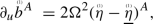  (2.39)
  

  (2.40)

• The equations governing the linearised connection coefficients (2.35):

  

  (2.41)
  

  (2.42)
  

  (2.43)
  

  (2.44)
  

  (2.45)
  

  (2.46)
  

  (2.47)
  

  (2.48)
  

  (2.49)

• The equations governing the curvature components (2.36):

  

  (2.50)
  

  (2.51)
  

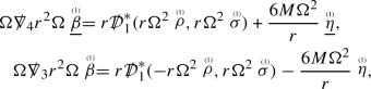  (2.52)
  

  (2.53)
  

  (2.54)

• Elliptic constraint equations: The linearised Codazzi equations

  

  (2.55)
  

  (2.56)
  

  (2.57)

  and the linearised Gauss equation

  

  (2.58)

Remark 2.2.1

The linearised Gaussian curvature is defined by

(2.59)

Remark 2.2.2

The degeneration of the Eddington–Finkelstein (EF) frame near $\overline{{\mathscr {H}}^+}$ carries over to a degeneration of the quantities governed by equations (2.41)–(2.54), as these quantities were derived via the EF frame (see Appendix B). By switching to a regular frame, e.g. the Kruskal frame, it can be shown that these quantities extend regularly to $\overline{{\mathscr {H}}^+}$ when supplied with the appropriate weights in U, V. In particular, note that

$$\begin{aligned} {\tilde{\alpha }}=V^{-2}\Omega ^2\alpha ,\qquad \underline{\widetilde{\alpha }}=U^2\Omega ^{-2}{\underline{\alpha }}, \end{aligned}$$

(2.60)

extend regularly to $\overline{{\mathscr {H}}^+}$, including ${\mathcal {B}}$.

3 The Teukolsky Equations, the Teukolsky–Starobinsky Identities and the Regge–Wheeler Equations

3.1 The Teukolsky equations and their well-posedness

Let , belong to a solution to the linearised Einstein equations (2.41)–(2.54). It turns out that the linearised fields , obey decoupled 2$^\mathrm{nd}$ order hyperbolic equations, the well-known Teukolsky equations.

Take the first equation of (2.50) and multiply by $\frac{r^4}{\Omega ^4}$:

(3.1)

Now differentiate in the $\Omega e_4$ direction and multiply by $\frac{\Omega ^2}{r^2}$ to obtain the Spin + 2 Teukolsky equation:

(3.2)

We note that:

(3.3)

We may rewrite the equation as:

(3.4)

An analogous procedure produces the Spin $\varvec{-2}$ Teukolsky equation

(3.5)

which we may rewrite as

(3.6)

We now state well-posedness theorems which are standard for linear second-order hyperbolic equations of the type that Eqs. (3.2), (3.5) fall under. Taking into account Remark 2.2.2, we start with the future evolution of $\Omega ^2\alpha$ and $\Omega ^{-2}{\underline{\alpha }}$.

Having derived the Teukolsky equations (3.2), (3.5), we can study these equations in isolation. Since the following theorems do not pertain to the linearised Einstein equations, we drop the superscript .

Proposition 3.1.1

Prescribe on $\Sigma ^*$ a pair of smooth symmetric traceless $S^2_{u,v}$ 2-tensor fields $(\upalpha ,\upalpha ')$. Then there exists a unique smooth symmetric traceless $S^2_{u,v}$ 2-tensor field $\Omega ^2\alpha$ that satisfies (3.2) on $J^+(\Sigma ^*)$, with .

Proposition 3.1.2

Prescribe on $\Sigma ^*$ a pair of smooth symmetric traceless $S^2_{u,v}$ 2-tensor fields $({\underline{\upalpha }},{\underline{\upalpha }}')$. Then there exists a unique smooth symmetric traceless $S^2_{u,v}$ 2-tensor field $\Omega ^{-2}{\underline{\alpha }}$ that satisfies (3.5) on $J^+(\Sigma ^*)$, with .

The same applies replacing $\Sigma ^*$ with any other ${\mathscr {H}}^+$-penetrating spacelike surface ending at $i^0$.

The degeneration of the EF frame discussed in Remark 2.2.2 is inherited by (3.2), (3.5), and we must work with $\widetilde{\alpha }=V^{-2}\Omega ^2\alpha , \widetilde{{\underline{\alpha }}}=U^2\Omega ^{-2}{\underline{\alpha }}$ in order to study the Teukolsky equations with data on $\overline{\Sigma }$. The weighted quantities $\widetilde{\alpha }, \widetilde{{\underline{\alpha }}}$ satisfy the following equations:

(3.7)

(3.8)

Equations (3.7) and (3.8) do not degenerate near ${\mathcal {B}}$ and we can make the following well-posedness statement:

Proposition 3.1.3

Prescribe a pair of smooth symmetric traceless $S^2_{U,V}$ 2-tensor fields $(\widetilde{\upalpha },\widetilde{\upalpha }')$ on $\overline{\Sigma }$. Then there exists a unique smooth symmetric traceless $S^2_{u,v}$ 2-tensor field $\Omega ^2{\alpha }$ that satisfies (3.2) on $J^+(\overline{\Sigma })$ with $V^{-2}\Omega ^2\alpha |_{\overline{\Sigma }}=\widetilde{\upalpha }$ and .

Proposition 3.1.4

Prescribe a pair of smooth symmetric traceless $S^2_{U,V}$ 2-tensor fields $(\widetilde{{\underline{\upalpha }}},\widetilde{{\underline{\upalpha }}}')$ on $\overline{\Sigma }$. Then there exists a unique smooth symmetric traceless $S^2_{u,v}$ 2-tensor field $\Omega ^{-2}{{\underline{\alpha }}}$ that satisfies (3.5) on $J^+(\overline{\Sigma })$ with $V^{2}\Omega ^{-2}{\underline{\alpha }}|_{\overline{\Sigma }}=\widetilde{{\underline{\upalpha }}}$ and .

Analogous statements to the above apply to past development from $\overline{\Sigma }$ with $U,\Omega ^2$ switching places with $V,\Omega ^{-2}$ respectively.

In developing backwards scattering we will use the following well-posedness statement for the past development of a mixed initial-characteristic value problem:

Proposition 3.1.5

Let $u_+<\infty , v_+<v_*<\infty$. Let $\widetilde{\Sigma }$ be a spacelike hypersurface connecting ${\mathscr {H}}^+$ at $v_+$ to ${\mathscr {I}}^+$ at $u_+$ and let $\underline{{\mathscr {C}}}=\underline{{\mathscr {C}}}_{v_*}\cap J^-(\widetilde{\Sigma })\cap J^+({\overline{\Sigma }})$. Prescribe a pair of symmetric traceless $S^2_{u,v}$ 2-tensor fields:

• $\alpha _{{{\mathscr {H}}^+}}$ on ${{\mathscr {H}}^+}\cap \{v\le v_+\}$ vanishing in a neighborhood of ${\mathscr {H}}^+\cap \{v=v_+\}$, such that $V^{-2}\alpha _{\overline{{\mathscr {H}}^+}}$ extends smoothly to ${\mathcal {B}}$,

• $\alpha _{0,in}$ on $\underline{{\mathscr {C}}}$ vanishing in a neighborhood of $\underline{{\mathscr {C}}}\cap \widetilde{\Sigma }$.

Then there exists a unique smooth symmetric traceless $S^2_{u,v}$ 2-tensor $\alpha$ on $D^-\left( \overline{{\mathscr {H}}^+}\cup \widetilde{\Sigma }\cup \underline{{\mathscr {C}}}\right) \cap J^+(\overline{\Sigma })$ satisfying the $+\,2$ Teukolsky equation (3.2) such that $V^{-2}\Omega ^2\alpha |_{\overline{{\mathscr {H}}^+}}=V^{-2}\alpha _{\overline{{\mathscr {H}}^+}}$, $\alpha |_{\underline{{\mathscr {C}}}}=\alpha _{0,in}$ and .

Proposition 3.1.6

Let $u_+<\infty , v_+<v_*<\infty$. Let $\widetilde{\Sigma }$ be a spacelike hypersurface connecting ${\mathscr {H}}^+$ at $v_+$ to ${\mathscr {I}}^+$ at $u_+$ and let $\underline{{\mathscr {C}}}=\underline{{\mathscr {C}}}_{v_*}\cap J^-(\widetilde{\Sigma })\cap \{t\ge 0\}$. Prescribe a pair of symmetric traceless $S^2_{u,v}$ 2-tensor fields:

• ${\underline{\alpha }}_{{{\mathscr {H}}^+}}$ on ${{\mathscr {H}}^+}\cap \{v<v_+\}$ vanishing in a neighborhood of $v_+$, such that $V^{2}{\underline{\alpha }}_{{{\mathscr {H}}^+}}$ extends smoothly to ${\mathcal {B}}$,

• ${\underline{\alpha }}_{0,in}$ on $\underline{{\mathscr {C}}}$ vanishing in a neighborhood of $\underline{{\mathscr {C}}}\cap \widetilde{\Sigma }$.

Then there exists a unique smooth symmetric traceless $S^2_{u,v}$ 2-tensor ${\underline{\alpha }}$ on $D^-\left( \overline{{\mathscr {H}}^+}\cup \widetilde{\Sigma }\cup \underline{{\mathscr {C}}}\right) \cap J^+(\overline{\Sigma })$ satisfying the $-\,2$ Teukolsky equation (3.5) such that $V^{2}\Omega ^{-2}{\underline{\alpha }}|_{\overline{{\mathscr {H}}^+}}=V^{2} {\underline{\alpha }}_{\overline{{\mathscr {H}}^+}}$, ${\underline{\alpha }}|_{\underline{{\mathscr {C}}}}={\underline{\alpha }}_{0,in}$ and .

We will also need

Proposition 3.1.7

Let ${\tilde{\alpha }}_{{\mathscr {H}}^+}$ be a smooth symmetric traceless $S^2_{\infty ,v}$ 2-tensor on $\overline{{\mathscr {H}}^+}\cap J^-(\Sigma ^*)$, $(\widetilde{\upalpha }_{\Sigma ^*},\widetilde{\upalpha }_{\Sigma ^*}')$ be a pair of smooth symmetric traceless $S^2_{\infty ,v}$ 2-tensors on $\Sigma ^*$. Then there exists a unique solution $\widetilde{\alpha }$ to (3.7) in $J^+(\overline{\Sigma })\cap \{t^*\le 0\}$ such that $\widetilde{\alpha }|_{\overline{{\mathscr {H}}^+}}=\widetilde{\alpha }_{\overline{{\mathscr {H}}^+}}$, .

Proposition 3.1.8

An analogous statement to Proposition 3.1.7 holds for Eq. (3.8).

Analogous statements apply for the "finite" backwards scattering problem from the past of $\overline{\Sigma }$, with U replacing V and $\Omega ^2$ switching places with $\Omega ^{-2}$.

Remark 3.1.1

(Time inversion) Under the transformation $t\longrightarrow -t$, $u\longrightarrow -v$ and $v\longrightarrow -u$ and thus and .

It is clear satisfies the $-\,2$ Teukolsky equation, i.e. the equation satisfied by ${\underline{\alpha }}$. Similarly, satisfies the $+\,2$ Teukolsky equation, i.e. the equation satisfied by $\alpha$. This observation means that the asymptotics of $\alpha$ towards the future are identical to those of ${\underline{\alpha }}$ towards the past, i.e. determining the asymptotics of both ${\underline{\alpha }}$ and $\alpha$ towards the future is enough to determine the asymptotics of either $\alpha$ or ${\underline{\alpha }}$ in both the past and future directions. We will use this fact to obtain bijective scattering maps from studying the forward evolution of the fields $\alpha ,{\underline{\alpha }}$. In particular, this prescription is sufficient to obtain well-posedness statements for the equations (3.5) and (3.2) for past development.

Remark 3.1.2

We will sometimes denote a field $\alpha$ satisfying the $+\,2$ Teukolsky equation by writing ${\mathcal {T}}^{+2}\alpha =0$. Similarly we may denote a solution ${\underline{\alpha }}$ to the $-\,2$ equation by ${\mathcal {T}}^{-2}\underline{\alpha }=0$.

3.2 Derivation of the Teukolsky–Starobinsky identities

We now return to the full system (2.41)–(2.54) to derive the Teukolsky–Starobinsky identities (1.5), (1.6).

Let belong to a solution of the linearised Einstein equations. Equation (2.50) implies:

(3.9)

Using (2.51) and (2.45) we obtain

(3.10)

We now apply to both sides and use equations (2.53), (2.54), (2.45) and the second equation of (2.44) to deduce

(3.11)

Now we apply once again and use (2.42), the second equation of (2.44) and the second equations of (2.48):

(3.12)

Finally, we have

(3.13)

An entirely analogous procedure starting from the equation for in (2.50) leads to

(3.14)

Equation (3.14) is the constraint (1.6).

3.3 Physical-space Chandrasekhar transformations and the Regge–Wheeler equation

The Regge–Wheeler equation for a symmetric traceless $S^2_{u,v}$ 2-tensor $\Psi$ is given by

(3.15)

Suppose the field $\alpha$ satisfies the $+\,2$ Teukolsky equation. Define the following hierarchy of fields

(3.16)

We have the following commutation relation:

(3.17)

where $a,b,c,k,k'$ are integers. We commute the operator past the Regge–Wheeler operator:

(3.18)

This shows that if $\alpha$ satisfies the $+\,2$ Teukolsky equation then $\Psi$ satisfies the Regge–Wheeler equation (3.15).

Analogously, with the following hierarchy of fields

(3.19)

we have

(3.20)

where $a,b,c,l,l'$ are integers. Thus, if ${\underline{\alpha }}$ satisfies the $-\,2$ Teukolsky equation then ${\underline{\Psi }}$ also satisfies the Regge–Wheeler equation.

We state a standard well-posedness result for (3.15):

Proposition 3.3.1

For any pair $(\uppsi ,\uppsi ')$ of smooth symmetric traceless $S^2_r$ 2-tensor fields on $\Sigma ^*$, there exists a unique smooth symmetric traceless $S^2_{u,v}$ 2-tensor field $\Psi$ which solves Eq. (3.15) in $J^+(\Sigma ^*)$ such that $\Psi |_{\Sigma ^*}=\uppsi$ and . The same applies when data are posed on $\Sigma$ or $\overline{\Sigma }$.

In contrast to the Teukolsky equations (3.2), (3.5), the Regge–Wheeler equation (3.15) does not suffer from additional regularity issues near ${\mathcal {B}}$, as can be seen by rewriting Eq. (3.15) in Kruskal coordinates:

(3.21)

If $\Psi$ is related to a field $\alpha$ that satisfies (3.2), then it is related to $\widetilde{\alpha }$ by

(3.22)

Proposition 3.3.2

Proposition 3.3.1 is valid replacing $\Sigma ^*$ with $\overline{\Sigma }$ everywhere.

For backwards scattering we will need the following well-posedness statement:

Proposition 3.3.3

Let $u_+<\infty , v_+<v_*<\infty$. Let $\widetilde{\Sigma }$ be a spacelike hypersurface connecting ${\mathscr {H}}^+$ at $v=v_+$ to ${\mathscr {I}}^+$ at $u=u_+$ and let $\underline{{\mathscr {C}}}=\underline{{\mathscr {C}}}_{v_*}\cap J^-(\widetilde{\Sigma })\cap \{t\ge 0\}$. Prescribe a pair of smooth symmetric traceless $S^2_{u,v}$ 2-tensor fields:

• $\Psi _{{{\mathscr {H}}^+}}$ on ${\overline{{\mathscr {H}}^+}}\cap \{v<v_+\}$ vanishing in a neighborhood of $\widetilde{\Sigma }$,

• $\Psi _{0,in}$ on $\underline{{\mathscr {C}}}$ vanishing in a neighborhood of $\widetilde{\Sigma }$.

Then there exists a unique smooth symmetric traceless $S^2_{u,v}$ 2-tensor $\Psi$ on $D^-\left( \overline{{\mathscr {H}}^+}\cup \widetilde{\Sigma }\cup \underline{{\mathscr {C}}}\right) \cap J^+(\overline{\Sigma })$ satisfying the Regge–Wheeler equation (3.15), such that $\Psi |_{\overline{{\mathscr {H}}^+}}=\Psi _{{{\mathscr {H}}^+}}$, $\Psi |_{\underline{{\mathscr {C}}}}=\Psi _{0,in}$ and .

We will also need

Proposition 3.3.4

Let $(\uppsi ,\uppsi ')$ be smooth symmetric traceless $S^2_{u,v}$ 2-tensor fields on $\Sigma ^*$, $\uppsi _{{\mathscr {H}}^+}$ be a smooth symmetric traceless $S^2_{\infty ,v}$ 2-tensor field on $\overline{{\mathscr {H}}^+}\cap \{t^*\le 0\}$. Then there exists a unique smooth symmetric traceless $S^2_{u,v}$ 2-tensor field $\Psi$ on $J^-(\Sigma ^*)$ such that .

Remark 3.3.1

Unlike the Teukolsky equations (3.2), (3.5), the Regge–Wheeler equation (3.15) is invariant under time inversion. If $\Psi (u,v)$ satisfies (3.15), then also satisfies (3.15).

3.4 Further constraints among $\alpha ,\Psi$ and ${\underline{\alpha }},{\underline{\Psi }}$

We can apply the same ideas as in Sect. 3.3 to transform solutions of the Regge–Wheeler equation into solutions of the $+\,2$ Teukolsky equation. Let $\Psi$ satisfy Eq. (3.15), then using (3.20) we can show that

(3.23)

satisfies Eq. (3.2).

Now suppose $\alpha$ satisfies Eq. (3.2) and $\Psi$ is the solution to Eq. (3.15) related to $\alpha$ by Eq. (3.16). We can evaluate the expression (3.23) using Eq. (3.2): we apply and substitute using the $+\,2$ equation only (we drop the superscript ):

(3.24)

i.e.,

(3.25)

We act on both sides with again:

(3.26)

We finally arrive at

(3.27)

We record the same for ${\underline{\Psi }}$: using only the Teukolsky equation (3.5) we obtain the analogue of (3.24)

(3.28)

and the analogue of (3.27)

(3.29)

In the remainder of this paper we focus exclusively on the Teukolsky equations (3.2), (3.5), the Teukolsky–Starobinsky identities (3.13), (3.14) and the Regge–Wheeler equation (3.15). In particular, we do not refer to the linearised Einstein equations (2.41)–(2.54) and as such, we drop the superscript .

Throughout this paper we will we distinguish between solutions arising from data on $\Sigma ^*, \Sigma$ or $\overline{\Sigma }$, and we subsequently construct separate scattering statements for each of these cases, in particular distinguishing between spaces of scattering states on ${\mathscr {H}}^+_{\ge 0}, {\mathscr {H}}^\pm$ and $\overline{{\mathscr {H}}^\pm }$. It will be easiest to work with data $\Sigma ^*$ first, and then the results for the remaining cases would follow easily.

4 Main Theorems

We define in this section the spaces of scattering states and provide a precise statement of the results. In what follows, $L^2$ spaces on ${\mathscr {I}}^\pm , {\mathscr {H}}^+_{\ge 0}, {\mathscr {H}}^\pm ,\overline{{\mathscr {H}}^\pm }$ are defined with respect to the measures $du\sin \theta d\theta d\phi$, $dv\sin \theta d\theta d\phi$ induced by the Eddington–Finkelstein coordinates.

Notation

For a spherically symmetric submanifold ${\mathcal {S}}$ of $\overline{{\mathscr {M}}}$, denote by $\Gamma ({\mathcal {S}})$ the space of smooth symmetric traceless $S^2_{u,v}$ 2-tensor fields on ${\mathcal {S}}$. The space of such fields that are compactly supported is denoted by $\Gamma _c ({\mathcal {S}})$. We use the same notation for smooth fields on ${\mathscr {I}}^\pm , {\mathscr {H}}^\pm ,\overline{{\mathscr {H}}^\pm }$.

In particular, note that $A\in \Gamma (\Sigma ^*)$ says that A is smooth up to and including $\Sigma ^*\cap {\mathscr {H}}^+$.

4.1 Theorem 1: Scattering for the Regge–Wheeler equation

Definition 4.1.1

Let $(\uppsi ,\uppsi ')\in \Gamma _c (\Sigma ^*)\oplus \Gamma _c(\Sigma ^*)$ be Cauchy data on $\Sigma ^*$ for (3.15) of compact support. Define the space ${\mathcal {E}}^{T}_{\Sigma ^*}$ to be the completion of $\Gamma _c (\Sigma ^*)$ data under the norm

(4.1)

where $\Psi$ is smooth and satisfies . The space ${\mathcal {E}}^T_{\Sigma }$ is similarly defined with the norm

(4.2)

Define the space ${\mathcal {E}}^T_{\Sigma }$ to be the completion of $\Gamma _{c}(\Sigma )$ data under the norm (4.2). The space ${\mathcal {E}}^{T}_{\overline{\Sigma }}$ and the norm $\Vert \;\Vert _{{\mathcal {E}}^T_{\overline{\Sigma }}}$ are similarly defined.

Remark 4.1.1

The kernel of $\Vert \;\;\Vert _{{\mathcal {E}}^T_{\Sigma ^*}}$ has trivial intersection with $\Gamma (\Sigma ^*)$. It suffices for a smooth data set $(\uppsi ,\uppsi ')$ to satisfy $\Vert (\uppsi ,\uppsi ')\Vert _{{\mathcal {E}}^T_{\Sigma ^*}}<\infty$ to have $(\uppsi ,\uppsi ')\in {\mathcal {E}}^T_{\Sigma ^*}$, so $\Vert \;\Vert _{{\mathcal {E}}^T_{\Sigma *}}, \Vert \;\Vert _{{\mathcal {E}}^T_{\Sigma }}, \Vert \;\Vert _{{\mathcal {E}}^T_{{\overline{\Sigma }}}}$ and (4.2) define normed spaces that can be extended to Hilbert spaces.

Definition 4.1.2

Define the space ${\mathcal {E}}_{{\mathscr {H}}^+_{\ge 0}}^{T}$ to be the completion of $\Gamma _c ({\mathscr {H}}^+_{\ge 0})$ under the norm

$$\begin{aligned} \Vert \Psi \Vert _{{\mathcal {E}}_{{\mathscr {H}}^+_{\ge 0}}^{T}}^2=\int _{{\mathscr {H}}^+_{\ge 0}}|\partial _v\Psi |^2\sin \theta d\theta d\phi dv. \end{aligned}$$

(4.3)

The spaces ${\mathcal {E}}^T_{{\mathscr {H}}^+}$, ${\mathcal {E}}^T_{\overline{{\mathscr {H}}^+}}$ are analogously defined.

Remark 4.1.2

• 1. The energy $\Vert \;\Vert _{{\mathcal {E}}_{{\mathscr {H}}^+_{\ge 0}}^{T}}$ indeed defines a norm on $\Gamma _c({\mathscr {H}}^+_{\ge 0})$, which thus extends to a Hilbert space ${\mathcal {E}}^{T}_{{\mathscr {H}}^+_{\ge 0}}$ when completed under $\Vert \;\Vert _{{\mathcal {E}}_{{\mathscr {H}}^+_{\ge 0}}^{T}}$. The same applies to ${\mathcal {E}}^T_{{\mathscr {H}}^+}, {\mathcal {E}}^T_{\overline{{\mathscr {H}}^+}}$.

• 2. The space ${\mathcal {E}}^{T}_{{\mathscr {H}}^+_{\ge 0}}$ can be realised as the subset $\Psi _{{\mathscr {H}}^+}\in L^2_{loc}({\mathscr {H}}^+_{\ge 0})$ such that

  • ,

  • $\lim _{v\longrightarrow \infty } \left| \Psi _{{\mathscr {H}}^+}\right| _{S_{\infty ,v}^2}=0$.

  Note that Hardy’s inequality holds on elements of this space and we have

  $$\begin{aligned} \int _{{\mathscr {H}}^+_{\ge 0}} dv \sin \theta d\theta d\phi \frac{|\Psi _{{\mathscr {H}}^+}|^2}{v^2+1}\lesssim \Vert \Psi _{{\mathscr {H}}^+}\Vert ^2_{{\mathcal {E}}^{T}_{{\mathscr {H}}^+_{\ge 0}}}<\infty . \end{aligned}$$

  (4.4)

Definition 4.1.3

Define the space ${\mathcal {E}}^T_{{\mathscr {I}}^+}$ to be the completion of $\Gamma _c({\mathscr {I}}^+)$ under the norm

$$\begin{aligned} \Vert \Psi \Vert _{{\mathcal {E}}_{{\mathscr {I}}^+}^{T}}^2= \int _{{\mathscr {I}}^+}|\partial _u\Psi |^2\sin \theta d\theta d\phi du. \end{aligned}$$

(4.5)

Definition 4.1.4

Define the space ${\mathcal {E}}_{{\mathscr {H}}^-}^{T}$ to be the completion of $\Gamma _c ({\mathscr {H}}^-)$ under the norm

$$\begin{aligned} \Vert \Psi \Vert _{{\mathcal {E}}_{{\mathscr {H}}^-}^{T}}^2=\int _{{\mathscr {H}}^-}|\partial _u\Psi |^2\sin \theta d\theta d\phi du. \end{aligned}$$

(4.6)

The space ${\mathcal {E}}^T_{\overline{{\mathscr {H}}^-}}$ is similarly defined.

Definition 4.1.5

Define the space ${\mathcal {E}}_{{\mathscr {I}}^-}^T$ to be the completion of $\Gamma _c({\mathscr {I}}^-)$ under the norm

$$\begin{aligned} \Vert \Psi \Vert _{{\mathcal {E}}^T_{{\mathscr {I}}^-}}^2=\int _{{\mathscr {I}}^-} |\partial _v \Psi |^2 dv\sin \theta d\theta d\phi . \end{aligned}$$

(4.7)

Remark 4.1.3

Similar statements to Remark 4.1.2 apply to the norms $\Vert \;\;\Vert _{{\mathcal {E}}^T_{{\mathscr {H}}^\pm }}, \Vert \;\;\Vert _{{\mathcal {E}}^T_{\overline{{\mathscr {H}}^\pm }}}, \Vert \;\;\Vert _{{\mathcal {E}}^T_{{\mathscr {I}}^\pm }}$; they are positive-definite on smooth, compactly supported data on the respective regions of $\overline{{\mathscr {M}}}$, thus they define normed spaces which extend to Hilbert spaces ${\mathcal {E}}^T_{{\mathscr {H}}_{\ge 0}}, {\mathcal {E}}^T_{{\mathscr {H}}^\pm }, {\mathcal {E}}^T_{\overline{{\mathscr {H}}^\pm }}, {\mathcal {E}}^T_{{\mathscr {I}}^\pm }$ upon completion. Elements of these spaces can be identified with tensor fields in $L^2_{loc}({\mathscr {H}}^-)$ for which a similar statement to (4.4) applies.

Theorem 4.1.1

Let $(\uppsi ,\uppsi ')\in \Gamma _c(\Sigma ^*)\times \Gamma _c(\Sigma ^*)$. Then the corresponding unique solution $\Psi$ to (3.15) given by Proposition 3.3.1 on $J^+(\Sigma ^*)$ induces smooth radiation fields $(\varvec{\uppsi }_{{\mathscr {H}}^+},\varvec{\uppsi }_{{\mathscr {I}}^+})\in \Gamma ({\mathscr {H}}^+_{\ge 0})\oplus \Gamma ({\mathscr {I}}^+)$ as in definitions 5.2.2 and 5.2.1, with $\varvec{\uppsi }_{{\mathscr {I}}^+}, \varvec{\Psi }_{{\mathscr {H}}^+}$ satisfying

$$\begin{aligned} \left| \left| (\uppsi ,\uppsi ')\right| \right| _{{\mathcal {E}}^T_{\Sigma ^*}}^2=\left| \left| \varvec{\uppsi }_{{\mathscr {I}}^+}\right| \right| _{{\mathcal {E}}^T_{{\mathscr {I}}^+}}^2+\left| \left| \varvec{\uppsi }_{{\mathscr {H}}^+}\right| \right| _{{\mathcal {E}}^T_{{\mathscr {H}}^+}}^2. \end{aligned}$$

(4.8)

This extends to a map

$$\begin{aligned} \mathscr {F}^+: {\mathcal {E}}^T_{\Sigma ^*}\longrightarrow {\mathcal {E}}^T_{{\mathscr {H}}^+_{\ge 0}}\oplus {\mathcal {E}}^T_{{\mathscr {I}}^+}. \end{aligned}$$

(4.9)

Analogously, forward evolution from smooth compactly supported data on $\Sigma$ or $\overline{\Sigma }$ extends to the maps,

(4.10)

(4.11)

Theorem 4.1.2

Let $\varvec{\uppsi }_{{\mathscr {I}}^+}\in \Gamma _c ({\mathscr {I}}^+), \varvec{\uppsi }_{{\mathscr {H}}^+} \in \Gamma _c ({\mathscr {H}}^+_{\ge 0})$. Then there exists a unique solution $\Psi$ to Eq. (3.15) in $J^+(\Sigma ^*)$ which is smooth, such that

$$\begin{aligned} \lim _{v\longrightarrow \infty } \Psi (u,v,\theta ^A)=\varvec{\uppsi }_{{\mathscr {I}}^+},\qquad \qquad \Psi \big |_{{\mathscr {H}}^+_{\ge 0}}=\varvec{\uppsi }_{{\mathscr {H}}^+}. \end{aligned}$$

(4.12)

with . This extends to a map

$$\begin{aligned} {\mathscr {B}}^-: {\mathcal {E}}^T_{{\mathscr {H}}^+_{\ge 0}}\oplus {\mathcal {E}}^T_{{\mathscr {I}}^+}\longrightarrow {\mathcal {E}}^T_{{\Sigma ^*}} , \end{aligned}$$

(4.13)

which inverts the map ${\mathscr {F}}^+$ of Theorem 4.1.1. Thus ${\mathscr {F}}^+, {\mathscr {B}}^+$ are unitary Hilbert space isomorphisms and

$$\begin{aligned} {\mathscr {B}}^-\circ {\mathscr {F}}^+={\mathscr {F}}^+\circ {\mathscr {B}}^+=Id. \end{aligned}$$

(4.14)

Similar statements apply to produce maps

(4.15)

(4.16)

Theorem 4.1.3

Analogously to Theorems 4.1.1 and 4.1.2, there exist bounded maps

$$\begin{aligned}&{\mathscr {F}}^-:{\mathcal {E}}^T_\Sigma \longrightarrow {\mathcal {E}}^T_{{\mathscr {H}}^-}\oplus {\mathcal {E}}^T_{{\mathscr {I}}^-},\qquad \qquad \qquad {\mathscr {B}}^+:{\mathcal {E}}^T_{{\mathscr {H}}^-}\oplus {\mathcal {E}}^T_{{\mathscr {I}}^-}\longrightarrow {\mathcal {E}}^T_\Sigma , \end{aligned}$$

(4.17)

$$\begin{aligned}&{\mathscr {F}}^-:{\mathcal {E}}^T_{\overline{\Sigma }}\longrightarrow {\mathcal {E}}^T_{\overline{{\mathscr {H}}^-}}\oplus {\mathcal {E}}^T_{{\mathscr {I}}^-},\qquad \qquad \qquad {\mathscr {B}}^+:{\mathcal {E}}^T_{\overline{{\mathscr {H}}^-}}\oplus {\mathcal {E}}^T_{{\mathscr {I}}^-}\longrightarrow {\mathcal {E}}^T_{{\overline{\Sigma }}}, \end{aligned}$$

(4.18)

such that ${\mathscr {F}}^-\circ {\mathscr {B}}^+={\mathscr {B}}^+\circ {\mathscr {F}}^-=Id$ on the respective domains. The maps

$$\begin{aligned}&{\mathscr {S}}={\mathscr {F}}^+\circ {\mathscr {B}}^+:{\mathcal {E}}^T_{{\mathscr {H}}^-}\oplus {\mathcal {E}}^T_{{\mathscr {I}}^-}\longrightarrow {\mathcal {E}}^T_{{\mathscr {H}}^+}\oplus {\mathcal {E}}^T_{{\mathscr {I}}^+}, \end{aligned}$$

(4.19)

$$\begin{aligned}&{\mathscr {S}}={\mathscr {F}}^+\circ {\mathscr {B}}^+:{\mathcal {E}}^T_{\overline{{\mathscr {H}}^-}}\oplus {\mathcal {E}}^T_{{\mathscr {I}}^-}\longrightarrow {\mathcal {E}}^T_{\overline{{\mathscr {H}}^+}}\oplus {\mathcal {E}}^T_{{\mathscr {I}}^+} \end{aligned}$$

(4.20)

constitute unitary Hilbert space isomorphism with inverses

$$\begin{aligned}&{\mathscr {S}}={\mathscr {F}}^-\circ {\mathscr {B}}^-:{\mathcal {E}}^T_{{\mathscr {H}}^+}\oplus {\mathcal {E}}^T_{{\mathscr {I}}^+}\longrightarrow {\mathcal {E}}^T_{{\mathscr {H}}^-}\oplus {\mathcal {E}}^T_{{\mathscr {I}}^-}, \end{aligned}$$

(4.21)

$$\begin{aligned}&{\mathscr {S}}={\mathscr {F}}^-\circ {\mathscr {B}}^-:{\mathcal {E}}^T_{\overline{{\mathscr {H}}^+}}\oplus {\mathcal {E}}^T_{{\mathscr {I}}^+}\longrightarrow {\mathcal {E}}^T_{\overline{{\mathscr {H}}^-}}\oplus {\mathcal {E}}^T_{{\mathscr {I}}^-} \end{aligned}$$

(4.22)

on the respective domains.

Remark 4.1.4

We emphasise that the spaces ${\mathcal {E}}^T_{\Sigma }$ and ${\mathcal {E}}^T_{\overline{\Sigma }}$ are different and ${\mathcal {E}}^T_{\Sigma }\subsetneq {\mathcal {E}}^T_{\overline{\Sigma }}$. Similarly, ${\mathcal {E}}^T_{{\mathscr {H}}^+}\subsetneq {\mathcal {E}}^T_{\overline{{\mathscr {H}}^+}}$. Our prescription in distinguishing between these spaces is consistent in the sense that elements of ${\mathcal {E}}^T_{\Sigma }$ are mapped into ${\mathcal {E}}^T_{{\mathscr {H}}^+}$ and vice versa. Our point of view is that the spaces ${\mathcal {E}}^T_{\overline{\Sigma }}, {\mathcal {E}}^T_{\overline{{\mathscr {H}}}^\pm }$ are the natural spaces to consider, since in these spaces scattering data are not restricted to vanish at the bifurcation sphere ${\mathcal {B}}$. It is however useful to have the statements involving ${\mathcal {E}}^T_{{\Sigma }}, {\mathcal {E}}^T_{{{\mathscr {H}}}^\pm }$. In particular, solutions arising from past scattering data identically vanishing on ${\mathscr {H}}^-$ will lie in these spaces.

4.2 Theorem 2: Scattering for the Teukolsky equations of spins $\pm \,2$

4.2.1 Scattering for the $+\,2$ Teukolsky equation

Definition 4.2.1

Let $(\upalpha ,\upalpha ')\in \Gamma _c(\Sigma ^*)\oplus \Gamma _c(\Sigma ^*)$ be Cauchy data for (3.2) on $\Sigma ^*$ giving rise to a solution $\alpha$. Define the space ${\mathcal {E}}^{T,+2}_{\Sigma ^*}$ to be the completion of $\Gamma _c(\Sigma ^*)\oplus \Gamma _c(\Sigma ^*)$ under the norm

(4.23)

where $\Psi$ is the weighted second derivative of $\alpha$. The spaces ${\mathcal {E}}^{T,+2}_{\Sigma }$, ${\mathcal {E}}^{T,+2}_{\overline{\Sigma }}$ are similarly defined.

We immediately note the following:

Proposition 4.2.1

$\Vert \;\Vert _{{\mathcal {E}}^{T,+2}_{\Sigma }}$ indeed defines a norm on $\Gamma _c(\Sigma )\times \Gamma _c(\Sigma )$. Similar statements hold for $\Vert \;\Vert _{{\mathcal {E}}^{T,+2}_{\Sigma ^*}}, \Vert \;\Vert _{{\mathcal {E}}^{T,+2}_{\overline{\Sigma }}}$.

Proof

It suffices to check that $\Vert (\upalpha ,\upalpha ')\Vert _{{\mathcal {E}}^{T,+2}_{\Sigma }}=0$ for a smooth, compactly supported pair $(\upalpha ,\upalpha ')$ implies that $(\upalpha ,\upalpha ')=(0,0)$. Let $\alpha$, $\Psi$ be as in Definition 4.2.1. It is clear that $\Psi =0$, and (3.27) implies:

(4.24)

Equation (3.24) implies that on $\Sigma$

(4.25)

Take $F=\left( {\mathcal {A}}_2-2+\frac{6M}{r}\right) r\Omega ^2\alpha$, then the above says . We integrate over the region $R_0<r<R$ on $\Sigma$:

(4.26)

This implies $\Vert F\Vert ^2_{S^2,r=R}\ge \Vert F\Vert ^2_{S^2,r=R_0}$ (notice that the integral on the right hand side remains positive by Poincaré’s inequality). If the data are compactly supported then F must vanish everywhere on $\Sigma$, and the vanishing of F implies the vanishing of $\Omega ^2\alpha$ for smooth $\alpha$ since the operator ${\mathcal {A}}_2-2+\frac{6M}{r}$ is uniformly elliptic on the set of symmetric, traceless 2-tensor field on $S^2$ (recall Remark 2.1.2). This in turn implies the vanishing of by (4.24). We can repeat this argument for data on $\Sigma ^*, \overline{\Sigma }$. $\quad \square$

Definition 4.2.2

Define the space of future scattering states ${\mathcal {E}}^{T,+2}_{{\mathscr {H}}^+_{\ge 0}}$ on ${\mathscr {H}}^+$ to be the completion of $\Gamma _c ({\mathscr {H}}^+_{\ge 0})$ under the norm

(4.27)

Define the space ${\mathcal {E}}^{T,+2}_{{\mathscr {H}}^+}$ to be the completion of $\Gamma _c({\mathscr {H}}^+)$ under the norm

$$\begin{aligned} \Vert A\Vert _{{\mathcal {E}}^{T,+2}_{{\mathscr {H}}^+}}&=\left\| {\mathcal {A}}_2({\mathcal {A}}_2-2)\left( \int _v^\infty d{\bar{v}}\; e^{\frac{1}{2M}(v-{\bar{v}})}A\right) \right\| ^2_{L^2({\mathscr {H}}^+)}\nonumber \\&\quad +\left\| 6M\partial _v\left( \int _v^\infty d{\bar{v}}\; e^{\frac{1}{2M}(v-{\bar{v}})}A\right) \right\| ^2_{L^2({\mathscr {H}}^+)}. \end{aligned}$$

(4.28)

Define the space ${\mathcal {E}}^{T,+2}_{\overline{{\mathscr {H}}^+}}$ to be the completion of the space consisting of symmetric traceless $S^2_{\infty ,v}$ 2-tensor fields A on $\overline{{\mathscr {H}}^+}$ such that $V^{-2}A\in \Gamma _c \left( \overline{{\mathscr {H}}^+}\right)$, under the same norm above evaluated over $\overline{{\mathscr {H}}^+}$.

Remark 4.2.1

Let $A\in \Gamma _c({\mathscr {H}}_{\ge 0}^+)$. If $\Vert A\Vert _{{\mathcal {E}}^{T,+2}_{{\mathscr {H}}^+_{\ge 0}}}=0$ then $\int _v^\infty d{\bar{v}}\; e^{\frac{1}{2M}(v-{\bar{v}})}A=0$ for all v, which implies that A must vanish if it is smooth. Thus $\Vert \;\Vert _{{\mathcal {E}}^{T,+2}_{{\mathscr {H}}^+_{\ge 0}}}$ defines a norm on $\Gamma _c({\mathscr {H}}^+_{\ge 0})$, which then extends to the Hilbert space ${\mathcal {E}}^{T,+2}_{{\mathscr {H}}^+_{\ge 0}}$. The same applies to ${\mathcal {E}}^{T,+2}_{{\mathscr {H}}^+}$, ${\mathcal {E}}^{T,+2}_{\overline{{\mathscr {H}}^+}}$.

Definition 4.2.3

Define the space of future scattering states ${\mathcal {E}}^{T,+2}_{{\mathscr {I}}^+}$ on ${\mathscr {I}}^+$ to be the completion of $\Gamma _c ({\mathscr {I}}^+)$ under the norm

$$\begin{aligned} \Vert A\Vert _{{\mathcal {E}}_{{\mathscr {I}}^+}^{T,+2}}=\left| \left| \partial _u^3A\right| \right| _{L^2({\mathscr {I}}^+)}. \end{aligned}$$

(4.29)

Remark 4.2.2

The energy $\Vert \;\Vert _{{\mathcal {E}}_{{\mathscr {I}}^+}^{T,+2}}$ indeed defines a norm on $\Gamma _c({\mathscr {I}}^+)$, which thus extends to a Hilbert space ${\mathcal {E}}^{T,+2}_{{\mathscr {I}}^+}$ when completed under $\Vert \;\Vert _{{\mathcal {E}}_{{\mathscr {I}}^+}^{T,+2}}$. We can identify ${\mathcal {E}}^{T,+2}_{{\mathscr {I}}^+}$ as the subset $A\in L^2_{loc}({\mathscr {I}}^+)$ whose elements satisfy

• $\partial _u^3 A\in L^2({\mathscr {I}}^+)$,

• $\lim _{u\longrightarrow \infty } \left| A\right| _{S^2}=0$.

Hardy’s inequality holds and we have on this subset

$$\begin{aligned} \int _{{\mathscr {I}}^+} du \sin \theta d\theta d\phi \frac{|A|^2}{u^6+1}\lesssim \Vert A\Vert ^2_{{\mathcal {E}}^{T,+2}_{{\mathscr {I}}^+}} <\infty . \end{aligned}$$

(4.30)

Definition 4.2.4

Define the space of past scattering states ${\mathcal {E}}^{T,+2}_{{\mathscr {H}}^-}$ on ${\mathscr {H}}^-$ to be the completion of $\Gamma _c ({\mathscr {H}}^-)$ under the norm

$$\begin{aligned} \Vert A\Vert _{{\mathcal {E}}^{T,+2}_{{\mathscr {H}}^-}}=\left| \left| 2(2M\partial _u)A-3(2M\partial _u)^2A+(2M\partial _u)^3A\right| \right| _{L^2({\mathscr {H}}^-)}. \end{aligned}$$

(4.31)

Define the space ${\mathcal {E}}^{T,+2}_{\overline{{\mathscr {H}}^-}}$ to be the closure of the space consisting of symmetric traceless $S^2_{u,-\infty }$ 2-tensor fields A on $\overline{{\mathscr {H}}^-}$ such that $U^2A\in \Gamma _c \left( \overline{{\mathscr {H}}^-}\right)$, under the same norm above evaluated over $\overline{{\mathscr {H}}^-}$.

Remark 4.2.3

As mentioned in Remark 2 of Section 1.3.2 of the introduction, the energy defined in (4.31) can be written using the Kruskal frame as

$$\begin{aligned} \Vert A\Vert _{{\mathcal {E}}^{T,+2}_{{\mathscr {H}}^-}}=\Vert U^{1/2}\partial _U^3U^2A\Vert _{L^2_UL^2(S^2)}. \end{aligned}$$

(4.32)

This defines a norm on $\Gamma _c({\mathscr {H}}^-)$, which then extends to the Hilbert space ${\mathcal {E}}^{T,+2}_{{\mathscr {H}}^-}$. It is possible to represent the elements of ${\mathcal {E}}^{T,+2}_{{\mathscr {H}}^-}$ as the subset $A\in L^2_{loc}({\mathscr {H}}^-)$ whose elements satisfy

• $\partial _uA$, $\partial _u^2 A$, $\partial _u^3 A \in L^2({\mathscr {H}}^-)$,

• $\lim _{u\longrightarrow -\infty } \Vert A\Vert _{L^2(S^2)}=0$

Hardy’s inequality holds on this space we have

$$\begin{aligned} \int _{{\mathscr {H}}^-} du \sin \theta d\theta d\phi \frac{|A|^2}{u^2+1}\lesssim \Vert A\Vert ^2_{{\mathcal {E}}^{T,+2}_{{\mathscr {H}}^-}}<\infty . \end{aligned}$$

(4.33)

Definition 4.2.5

Define the space of past scattering states ${\mathcal {E}}^{T,+2}_{{\mathscr {I}}^-}$ on ${\mathscr {I}}^-$ to be the completion of the space

$$\begin{aligned} A\in \Gamma ({\mathscr {I}}^-): \int _{-\infty }^\infty dv\;A=0 \end{aligned}$$

(4.34)

under the norm

$$\begin{aligned} \Vert A\Vert ^2_{{\mathcal {E}}^{T,+2}_{{\mathscr {I}}^-}}=&\int _{{\mathscr {I}}^-} d{\bar{v}}\sin \theta d\theta d\phi \left[ 6M|A|^2+\left| {\mathcal {A}}_2({\mathcal {A}}_2-2)\int _{{\bar{v}}}^\infty A\right| ^2\right] . \end{aligned}$$

(4.35)

Remark 4.2.4

Let $A\in \Gamma _c({\mathscr {I}}^-)$. If $\Vert A\Vert ^2_{{\mathcal {E}}^{T,+2}_{{\mathscr {I}}^-}}=0$ then $A=0$. Thus $\Vert \;\Vert ^2_{{\mathcal {E}}^{T,+2}_{{\mathscr {I}}^-}}$ defines a norm on $\Gamma _c({\mathscr {I}}^-)$ which then extends to the Hilbert space ${\mathcal {E}}^{T,+2}_{{\mathscr {I}}^-}$.

Theorem 4.2.2

Forward evolution under the $+\,2$ Teukolsky equation (3.2) from smooth, compactly supported data $(\upalpha ,\upalpha ')$ on $\Sigma ^*$ gives rise to smooth radiation fields $(\upalpha _{{\mathscr {H}}^+},\upalpha _{{\mathscr {I}}^+})\in {\mathcal {E}}^{T,+2}_{{\mathscr {H}}^+_{\ge 0}}\oplus {\mathcal {E}}^{T,+2}_{{\mathscr {I}}^+}$ where

• 1. $\upalpha _{{\mathscr {H}}^+}=2M\Omega ^{2}{\alpha }\big |_{{\mathscr {H}}^+} \in \Gamma ({\mathscr {H}}^+)$,

• 2. $\upalpha _{{\mathscr {I}}^+}=\lim _{v\longrightarrow \infty } r^5\alpha (v,u,\theta ^A)$, with $\upalpha _{{\mathscr {I}}^+}\in \Gamma ({\mathscr {I}}^+)$,

with $\upalpha _{{\mathscr {I}}^+}, \alpha _{{\mathscr {H}}^+}$ satisfying

$$\begin{aligned} \left| \left| (\upalpha ,\upalpha ')\right| \right| _{{\mathcal {E}}^{T,+2}_{\Sigma ^*}}^2=\left| \left| \upalpha _{{\mathscr {I}}^+}\right| \right| _{{\mathcal {E}}^{T,+2}_{{\mathscr {I}}^+}}^2+\left| \left| \upalpha _{{\mathscr {H}}^+}\right| \right| _{{\mathcal {E}}^{T,+2}_{{\mathscr {H}}^+_{\ge 0}}}^2. \end{aligned}$$

(4.36)

This extends to a unitary map

$$\begin{aligned} {}^{(+2)}\mathscr {F}^+: {\mathcal {E}}^{T,+2}_{\Sigma ^*}\longrightarrow {\mathcal {E}}^{T,+2}_{{\mathscr {H}}^+_{\ge 0}}\oplus {\mathcal {E}}^{T,+2}_{{\mathscr {I}}^+}. \end{aligned}$$

(4.37)

The same conclusions apply when replacing $\Sigma ^*$ with $\Sigma$ and ${\mathscr {H}}^+_{\ge 0}$ with ${\mathscr {H}}^+$, or when replacing with ${\overline{\Sigma }}$ and $\overline{{\mathscr {H}}^+}$. In the latter case, $(\upalpha ,\upalpha ')$ must be consistent with the well-posedness statement Proposition 3.1.1 and consequently we obtain that $V^{-2}\upalpha _{{{\mathscr {H}}^+}}\in \Gamma (\overline{{\mathscr {H}}^+})$.

Theorem 4.2.3

Let $\upalpha _{{\mathscr {I}}^+}\in \Gamma _c ({\mathscr {I}}^+), \upalpha _{{\mathscr {H}}^+} \in \Gamma _c ({\mathscr {H}}^+_{\ge 0})$. There exists a unique solution $\alpha$ to Eq. (3.2) in $J^+(\Sigma ^*)$ which is smooth, such that

$$\begin{aligned} \lim _{v\longrightarrow \infty } r^5\alpha (u,v,\theta ^A)=\upalpha _{{\mathscr {I}}^+},\qquad \qquad \Omega ^{2}\alpha \big |_{{\mathscr {H}}^+_{\ge 0}}=\upalpha _{{\mathscr {H}}^+}, \end{aligned}$$

(4.38)

with and . This extends to a unitary map

$$\begin{aligned} {}^{(+2)}{\mathscr {B}}^-: {\mathcal {E}}^{T,+2}_{{\mathscr {H}}^+_{\ge 0}}\oplus {\mathcal {E}}^{T,+2}_{{\mathscr {I}}^+}\longrightarrow {\mathcal {E}}^{T,+2}_{{\Sigma ^*}}, \end{aligned}$$

(4.39)

which inverts the map ${}^{(+2)}{\mathscr {F}}^+$ of Theorem 4.2.2

$$\begin{aligned} {}^{(+2)}{\mathscr {B}}^-\circ {}^{(+2)}{\mathscr {F}}^+={}^{(+2)}{\mathscr {F}}^+\circ {}^{(+2)}{\mathscr {B}}^-=Id. \end{aligned}$$

(4.40)

The same conclusions apply when replacing $\Sigma ^*$ with $\Sigma$ and ${\mathscr {H}}^+_{\ge 0}$ with ${\mathscr {H}}^+$, or when replacing with ${\overline{\Sigma }}$ and $\overline{{\mathscr {H}}^+}$. In the latter case, we require that $V^{-2}\alpha _{{{\mathscr {H}}^+}}\in \Gamma (\overline{{\mathscr {H}}^+})$ and thus the induced data satisfy the conditions of Proposition 3.1.3.

Theorem 4.2.4

Evolution from $(\upalpha ,\upalpha ')\in \Gamma _c(\Sigma )\times \Gamma _c(\Sigma )$ to $J^-(\Sigma )$ gives rise to radiation fields on ${\mathscr {H}}^-,{\mathscr {I}}^-$ analogously to Theorem 4.2.2, where the radiation fields are defined by

$$\begin{aligned} \lim _{u\longrightarrow -\infty } r\alpha (u,v,\theta ^A)=\upalpha _{{\mathscr {I}}^-},\qquad \qquad 2M\Omega ^{-2}\alpha \big |_{{\mathscr {H}}^-}=\upalpha _{{\mathscr {H}}^-}. \end{aligned}$$

(4.41)

This extends to a unitary map

$$\begin{aligned} {}^{(+2)}\mathscr {F}^-: {\mathcal {E}}^{T,+2}_{\Sigma }\longrightarrow {\mathcal {E}}^{T,+2}_{{\mathscr {H}}^-}\oplus {\mathcal {E}}^{T,+2}_{{\mathscr {I}}^-}, \end{aligned}$$

(4.42)

with inverse ${}^{(+2)}{\mathscr {B}}^+:{\mathcal {E}}^{T,+2}_{{\mathscr {H}}^-}\oplus {\mathcal {E}}^{T,+2}_{{\mathscr {I}}^-}\longrightarrow {\mathcal {E}}^{T,+2}_{\Sigma }$. The same conclusions apply when replacing $\Sigma$ with $\overline{\Sigma }$ and ${\mathscr {H}}^-$ with $\overline{{\mathscr {H}}^-}$. In this case, we require that $(U^{2}\Omega ^{-2}\upalpha ,U^{2}\Omega ^{-2}\upalpha ')$ are smooth up to and including ${\mathcal {B}}$, and consequently we obtain that $U^{2}\upalpha _{{{\mathscr {H}}^-}}\in \Gamma (\overline{{\mathscr {H}}^-})$.

Theorem 4.2.5

The maps

$$\begin{aligned} {}^{(+2)}{\mathscr {S}}&={}^{(+2)}{\mathscr {F}}^+\circ {}^{(+2)}{\mathscr {B}}^+:{\mathcal {E}}^{T,+2}_{{\mathscr {H}}^-}\oplus {\mathcal {E}}^{T,+2}_{{\mathscr {I}}^-}\longrightarrow {\mathcal {E}}^{T,+2}_{{\mathscr {H}}^+}\oplus {\mathcal {E}}^{T,+2}_{{\mathscr {I}}^+}, \end{aligned}$$

(4.43)

$$\begin{aligned} {}^{(+2)}{\mathscr {S}}&={}^{(+2)}{\mathscr {F}}^+\circ {}^{(+2)}{\mathscr {B}}^+:{\mathcal {E}}^{T,+2}_{\overline{{\mathscr {H}}^-}}\oplus {\mathcal {E}}^{T,+2}_{{\mathscr {I}}^-}\longrightarrow {\mathcal {E}}^{T,+2}_{\overline{{\mathscr {H}}^+}}\oplus {\mathcal {E}}^{T,+2}_{{\mathscr {I}}^+} \end{aligned}$$

(4.44)

constitute unitary Hilbert space isomorphism with inverses

$$\begin{aligned} {}^{(+2)}{\mathscr {S}}^-&={}^{(+2)}{\mathscr {F}}^-\circ {}^{(+2)}{\mathscr {B}}^-:{\mathcal {E}}^{T,+2}_{{\mathscr {H}}^+}\oplus {\mathcal {E}}^{T,+2}_{{\mathscr {I}}^+}\longrightarrow {\mathcal {E}}^{T,+2}_{{\mathscr {H}}^-}\oplus {\mathcal {E}}^{T,+2}_{{\mathscr {I}}^-} \end{aligned}$$

(4.45)

$$\begin{aligned} {}^{(+2)}{\mathscr {S}}^-&={}^{(+2)}{\mathscr {F}}^-\circ {}^{(+2)}{\mathscr {B}}^-:{\mathcal {E}}^{T,+2}_{\overline{{\mathscr {H}}^+}}\oplus {\mathcal {E}}^{T,+2}_{{\mathscr {I}}^+}\longrightarrow {\mathcal {E}}^{T,+2}_{\overline{{\mathscr {H}}^-}}\oplus {\mathcal {E}}^{T,+2}_{{\mathscr {I}}^-} \end{aligned}$$

(4.46)

on the respective domains.

4.2.2 Scattering for the $-\,2$ Teukolsky equation

Definition 4.2.6

Let $({\underline{\upalpha }},{\underline{\upalpha }}')\in \Gamma _c(\Sigma ^*)\oplus \Gamma _c(\Sigma ^*)$ be Cauchy data for (3.2) on $\Sigma ^*$ giving rise to a solution ${\underline{\alpha }}$. Define the space ${\mathcal {E}}^{T,-2}_{\Sigma ^*}$ to be the completion of $\Gamma _c(\Sigma ^*)\oplus \Gamma _c(\Sigma ^*)$ under the norm

(4.47)

where ${\underline{\Psi }}$ is the weighted second derivative of ${\underline{\alpha }}$. The spaces ${\mathcal {E}}^{T,-2}_{\Sigma }$, ${\mathcal {E}}^{T,-2}_{\overline{\Sigma }}$ are similarly defined.

Proposition 4.2.6

$\Vert \;\Vert _{{\mathcal {E}}^{T,-2}_{\Sigma }}$ indeed defines a norm on $\Gamma _c(\Sigma )\times \Gamma _c(\Sigma )$.

Proof

It suffices to check that $\Vert ({\underline{\upalpha }},{\underline{\upalpha }}')\Vert _{{\mathcal {E}}^{T,-2}_{\Sigma }}=0$ implies $({\underline{\upalpha }},{\underline{\upalpha }}')=(0,0)$. Let ${\underline{\alpha }}$ and ${\underline{\Psi }}$ be as in Definition 4.2.6. It is clear that $\Vert ({\underline{\upalpha }},{\underline{\upalpha }}')\Vert _{{\mathcal {E}}^{T,-2}_{\Sigma }}=0$ implies $\Psi =0$. Equation (3.29) implies that

(4.48)

Equation (3.28) then gives us

(4.49)

Let , then (4.49) above implies that . The result follows similarly to Proposition 4.2.1. $\quad \square$

Definition 4.2.7

Define the space of future scattering states ${\mathcal {E}}^{T,-2}_{{\mathscr {H}}^+_{\ge 0}}$ on ${\mathscr {H}}^+_{\ge 0}$ to be the completion of $\Gamma _c({\mathscr {H}}^+_{\ge 0})$ under the norm

$$\begin{aligned} \Vert {\underline{A}}\Vert _{{\mathcal {E}}^{T,-2}_{{\mathscr {H}}^+_{\ge 0}}}=(2M)^2\left| \left| 2(2M\partial _v){\underline{A}}+3(2M\partial _v)^2{\underline{A}}+(2M\partial _v)^3{\underline{A}}\right| \right| _{L^2({\mathscr {H}}^+_{\ge 0})}. \end{aligned}$$

(4.50)

The space ${\mathcal {E}}^{T,-2}_{{\mathscr {H}}^+}$ is defined by the same norm taken over ${\mathscr {H}}^+$. Define and ${\mathcal {E}}^{T,-2}_{\overline{{\mathscr {H}}^+}}$ to be the closure of the space consisting of symmetric traceless $S^2_{\infty ,v}$ 2-tensor fields ${\underline{A}}$ on $\overline{{\mathscr {H}}^+}$ such that $V^{2}{\underline{A}}\in \Gamma _c \left( \overline{{\mathscr {H}}^+}\right)$, under the same norm above evaluated over $\overline{{\mathscr {H}}^+}$.

Remark 4.2.5

As with Remark 4.2.3 on $\Vert \;\Vert _{{\mathcal {E}}^{T,+2}_{{\mathscr {H}}^-}}$, the energy $\Vert \;\Vert _{{\mathcal {E}}^{T,-2}_{{\mathscr {H}}^+}}$ indeed defines a norm on $\Gamma _c(\overline{{\mathscr {H}}^+})$, which then extends to the Hilbert space ${\mathcal {E}}^{T,-2}_{\overline{{\mathscr {H}}^+}}$. It is possible to represent the elements of ${\mathcal {E}}^{T,-2}_{{\mathscr {H}}^+_{\ge 0}}$ as the subset ${\underline{A}}\in L^2_{loc}({\mathscr {H}}^+_{\ge 0})$ whose elements satisfy

• $\partial _v {\underline{A}}$, $\partial _v^2 {\underline{A}}$, $\partial _v^3 A \in L^2({\mathscr {H}}^+_{\ge 0})$,

• $\lim _{v\longrightarrow \infty } \Vert {\underline{A}}\Vert _{L^2(S^2)}=0$

Hardy’s inequality holds on this space we have

$$\begin{aligned} \int _{{\mathscr {H}}^+_{\ge 0}} dv \sin \theta d\theta d\phi \frac{|{\underline{A}}|^2}{v^2+1}\lesssim \Vert {\underline{A}}\Vert ^2_{{\mathcal {E}}^{T,-2}_{{\mathscr {H}}^+_{\ge 0}}}<\infty . \end{aligned}$$

(4.51)

Similar statements apply to ${\mathcal {E}}^{T,-2}_{{{\mathscr {H}}^+}}$, ${\mathcal {E}}^{T,-2}_{\overline{{\mathscr {H}}^+}}$.

Definition 4.2.8

Define the space of future scattering states ${\mathcal {E}}^{T,-2}_{{\mathscr {I}}^+}$ on ${\mathscr {I}}^+$ to be the completion of the space

$$\begin{aligned} {\underline{A}}\in \Gamma _c ({\mathscr {I}}^+):&\int _{-\infty }^{\infty } du{\underline{A}}=0 \end{aligned}$$

(4.52)

under the norm

$$\begin{aligned} \Vert {\underline{A}}\Vert ^2_{{\mathcal {E}}^{T,-2}_{{\mathscr {I}}^+}}=&\int _{{\mathscr {I}}^+} d{u}\sin \theta d\theta d\phi \left[ (6M)^2|{\underline{A}}|^2+\left| {\mathcal {A}}_2({\mathcal {A}}_2-2)\int _{{\bar{u}}}^\infty d{\bar{u}}\; {\underline{A}}\right| ^2\right] . \end{aligned}$$

(4.53)

Remark 4.2.6

As with $\Vert \;\Vert _{{\mathcal {E}}^{T,+2}_{{\mathscr {I}}^-}}$ and Remark 4.2.2, the energy $\Vert \;\Vert _{{\mathcal {E}}^{T,-2}_{{\mathscr {I}}^+}}$ indeed defines a norm on $\Gamma _c({{\mathscr {I}}^+})$, which then extends to the Hilbert space ${\mathcal {E}}^{T,-2}_{{{\mathscr {I}}^+}}$.

Definition 4.2.9

Define the space ${\mathcal {E}}^{T,-2}_{{\mathscr {H}}^-}$ to be the completion of $\Gamma _c({\mathscr {H}}^-)$ under the norm

$$\begin{aligned} \Vert {\underline{A}}\Vert _{{\mathcal {E}}^{T,-2}_{{\mathscr {H}}^-}}=&\left\| {\mathcal {A}}_2({\mathcal {A}}_2-2)\left( \int ^u_{-\infty } d{\bar{u}}\; e^{\frac{1}{2M}(u-{\bar{u}})}{\underline{A}}\right) \right\| ^2_{L^2({\mathscr {H}}^-)}\nonumber \\&+\left\| 6M\partial _u\left( \int ^u_{-\infty } d{\bar{u}}\; e^{\frac{1}{2M}(u-{\bar{u}})}{\underline{A}}\right) \right\| ^2_{L^2({\mathscr {H}}^-)}. \end{aligned}$$

(4.54)

Define the space ${\mathcal {E}}^{T,-2}_{\overline{{\mathscr {H}}^-}}$ to be the completion of the space consisting of symmetric traceless $S^2_{u,-\infty }$ 2-tensor fields ${\underline{A}}$ on $\overline{{\mathscr {H}}^-}$ such that $U^{-2}A\in \Gamma _c \left( \overline{{\mathscr {H}}^-}\right)$, under the same norm above evaluated over $\overline{{\mathscr {H}}^-}$.

Remark 4.2.7

As with $\Vert \;\Vert _{{\mathcal {E}}^{T,-2}_{\overline{{\mathscr {H}}^-}}}$ and Remark 4.2.7, the energy $\Vert \;\Vert _{{\mathcal {E}}^{T,-2}_{\overline{{\mathscr {H}}^-}}}$ indeed defines a norm on $\Gamma _c(\overline{{\mathscr {H}}^-})$, which then extends to the Hilbert space ${\mathcal {E}}^{T,-2}_{\overline{{\mathscr {H}}^-}}$.

Definition 4.2.10

Define the space of future scattering states ${\mathcal {E}}^{T,-2}_{{\mathscr {I}}^-}$ on ${\mathscr {I}}^-$ to be the completion of $\Gamma _c ({\mathscr {I}}^-)$ under the norm

$$\begin{aligned} \Vert {\underline{A}}\Vert _{{\mathcal {E}}_{{\mathscr {I}}^-}^{T,-2}}=\left| \left| \partial _v^3{\underline{A}}\right| \right| _{L^2({\mathscr {I}}^-)}. \end{aligned}$$

(4.55)

Remark 4.2.8

The energy $\Vert \;\Vert _{{\mathcal {E}}_{{\mathscr {I}}^-}^{T,-2}}$ indeed defines a norm on $\Gamma _c({\mathscr {I}}^-)$, which thus extends to a Hilbert space ${\mathcal {E}}^{T,-2}_{{\mathscr {I}}^-}$ when completed under $\Vert \;\Vert _{{\mathcal {E}}_{{\mathscr {I}}^-}^{T,-2}}$. We can identify ${\mathcal {E}}^{T,-2}_{{\mathscr {I}}^-}$ as the subset $A\in L^2_{loc}({\mathscr {I}}^-)$ whose elements satisfy

• $\partial _v {\underline{A}}$, $\partial _v^2 {\underline{A}}$, $\partial _v^3 {\underline{A}}\in L^2({\mathscr {I}}^-)$,

• $\lim _{v\longrightarrow -\infty } \Vert {\underline{A}}\Vert _{L^2(S^2)}=0$.

Hardy’s inequality holds and we have on this subset

$$\begin{aligned} \int _{{\mathscr {I}}^-} dv \sin \theta d\theta d\phi \frac{|{\underline{A}}|^2}{v^6+1}\lesssim \Vert {\underline{A}}\Vert ^2_{{\mathcal {E}}^{T,-2}_{{\mathscr {I}}^-}} <\infty . \end{aligned}$$

(4.56)

Theorem 4.2.7

Forward evolution under the $-\,2$ Teukolsky equation (3.5) from smooth, compactly supported data $({\underline{\upalpha }},{\underline{\upalpha }}')$ on $\Sigma ^*$ gives rise to smooth radiation fields $({\underline{\upalpha }}_{{\mathscr {H}}^+},{\underline{\upalpha }}_{{\mathscr {I}}^+})\in {\mathcal {E}}^{T,-2}_{{\mathscr {H}}^+_{\ge 0}}\oplus {\mathcal {E}}^{T,-2}_{{\mathscr {I}}^+}$ where

• 1. ${\underline{\upalpha }}_{{\mathscr {H}}^+}=2M\Omega ^{-2}{{\underline{\alpha }}}\big |_{{\mathscr {H}}^+} \in \Gamma ({\mathscr {H}}^+)$,

• 2. ${\underline{\upalpha }}_{{\mathscr {I}}^+}=\lim _{v\longrightarrow \infty } r{\underline{\alpha }}(v,u,\theta ^A)$, with ${\underline{\upalpha }}_{{\mathscr {I}}^+}\in \Gamma ({\mathscr {I}}^+)$,

with ${\underline{\upalpha }}_{{\mathscr {I}}^+}, {\underline{\upalpha }}_{{\mathscr {H}}^+}$ satisfying

$$\begin{aligned} \left| \left| ({\underline{\upalpha }},{\underline{\upalpha }}')\right| \right| _{{\mathcal {E}}^{T,-2}_{\Sigma ^*}}^2=\left| \left| \underline{\upalpha }_{{\mathscr {I}}^+}\right| \right| _{{\mathcal {E}}^{T,-2}_{{\mathscr {I}}^+}}^2+\left| \left| \underline{\upalpha }_{{\mathscr {H}}^+}\right| \right| _{{\mathcal {E}}^{T,-2}_{{\mathscr {H}}^+_{\ge 0}}}^2. \end{aligned}$$

(4.57)

This extends to a unitary map

$$\begin{aligned} {}^{(-2)}\mathscr {F}^+: {\mathcal {E}}^{T,-2}_{\Sigma ^*}\longrightarrow {\mathcal {E}}^{T,-2}_{{\mathscr {H}}^+_{\ge 0}}\oplus {\mathcal {E}}^{T,-2}_{{\mathscr {I}}^+}. \end{aligned}$$

(4.58)

The same conclusions apply when replacing $\Sigma ^*$ with $\Sigma$ and ${\mathscr {H}}^+_{\ge 0}$ with ${\mathscr {H}}^+$, or when replacing with ${\overline{\Sigma }}$ and $\overline{{\mathscr {H}}^+}$. In the latter case, $({\underline{\upalpha }},{\underline{\upalpha }}')$ must be consistent with the well-posedness statement Proposition 3.1.2 and consequently we obtain that $V^{2}{\underline{\upalpha }}_{{{\mathscr {H}}^+}}\in \Gamma (\overline{{\mathscr {H}}^+})$.

Theorem 4.2.8

Let ${\underline{\upalpha }}_{{\mathscr {I}}^+}\in \Gamma _c ({\mathscr {I}}^+), {\underline{\upalpha }}_{{\mathscr {H}}^+} \in \Gamma _c ({\mathscr {H}}^+_{\ge 0})$ with $\int _{-\infty }^\infty d{\bar{u}}\; {\underline{\upalpha }}_{{\mathscr {I}}^+}=0$. Then there exists a unique solution ${\underline{\alpha }}$ to Eq. (3.5) in $J^+(\Sigma ^*)$ which is smooth, such that

$$\begin{aligned} \lim _{v\longrightarrow \infty } r{\underline{\alpha }}(u,v,\theta ^A)={\underline{\upalpha }}_{{\mathscr {I}}^+},\qquad \qquad 2M\Omega ^{-2}{\underline{\alpha }}\big |_{{\mathscr {H}}^+_{\ge 0}}={\underline{\upalpha }}_{{\mathscr {H}}^+}, \end{aligned}$$

(4.59)

with and . This extends to a unitary map

$$\begin{aligned} {}^{(-2)}{\mathscr {B}}^-: {\mathcal {E}}^{T,-2}_{{\mathscr {H}}^+_{\ge 0}}\oplus {\mathcal {E}}^{T,-2}_{{\mathscr {I}}^+}\longrightarrow {\mathcal {E}}^{T,-2}_{{\Sigma ^*}}, \end{aligned}$$

(4.60)

which inverts the map ${}^{(-2)}{\mathscr {F}}^+$ of Theorem 4.2.7

$$\begin{aligned} {}^{(-2)}{\mathscr {B}}^-\circ {}^{(-2)}{\mathscr {F}}^+={}^{(-2)}{\mathscr {F}}^+\circ {}^{(-2)}{\mathscr {B}}^-=Id. \end{aligned}$$

(4.61)

The same conclusions apply when replacing $\Sigma ^*$ with $\Sigma$ and ${\mathscr {H}}^+_{\ge 0}$ with ${\mathscr {H}}^+$, or when replacing with ${\overline{\Sigma }}$ and $\overline{{\mathscr {H}}^+}$. In the latter case, we require that $V^2{\underline{\upalpha }}_{{{\mathscr {H}}^+}}\in \Gamma (\overline{{\mathscr {H}}^+})$ and with that is consistent with Proposition 3.1.2

Theorem 4.2.9

Evolution from $({\underline{\upalpha }},{\underline{\upalpha }}')\in \Gamma _c(\Sigma )\times \Gamma _c(\Sigma )$ to $J^-(\Sigma )$ gives rise to radiation fields on ${\mathscr {H}}^-,{\mathscr {I}}^-$ analogously to Theorem 4.2.2, where the radiation fields are defined by

$$\begin{aligned} \lim _{v\longrightarrow \infty } r^5{\underline{\alpha }}(u,v,\theta ^A)={\underline{\upalpha }}_{{\mathscr {I}}^-}\qquad \qquad 2M\Omega ^{2}{\underline{\alpha }}\big |_{{\mathscr {H}}^-}={\underline{\upalpha }}_{{\mathscr {H}}^-} \end{aligned}$$

(4.62)

This extends to a unitary map

$$\begin{aligned} {}^{(-2)}\mathscr {F}^-: {\mathcal {E}}^{T,-2}_{\Sigma }\longrightarrow {\mathcal {E}}^{T,-2}_{{\mathscr {H}}^-}\oplus {\mathcal {E}}^{T,-2}_{{\mathscr {I}}^-} \end{aligned}$$

(4.63)

with inverse ${}^{(-2)}{\mathscr {B}}^+:{\mathcal {E}}^{T,-2}_{{\mathscr {H}}^-}\oplus {\mathcal {E}}^{T,-2}_{{\mathscr {I}}^-}\longrightarrow {\mathcal {E}}^{T,-2}_{\Sigma }$. The same conclusions apply when replacing $\Sigma$ with $\overline{\Sigma }$ and ${\mathscr {H}}^-$ with $\overline{{\mathscr {H}}^-}$. In this case, we require that $(U^{-2}\Omega ^2{\underline{\alpha }},U^{-2}\Omega ^2{\underline{\alpha }}')$ are smooth up to and including ${\mathcal {B}}$, and consequently we obtain that $U^{-2}{\underline{\alpha }}_{{{\mathscr {H}}^+}}\in \Gamma (\overline{{\mathscr {H}}^+})$

Theorem 4.2.10

The maps

$$\begin{aligned}&{}^{(-2)}{\mathscr {S}}^+={}^{(-2)}{\mathscr {F}}^+\circ {}^{(-2)}{\mathscr {B}}^+:{\mathcal {E}}^{T,-2}_{{\mathscr {H}}^-}\oplus {\mathcal {E}}^{T,-2}_{{\mathscr {I}}^-}\longrightarrow {\mathcal {E}}^{T,-2}_{{\mathscr {H}}^+}\oplus {\mathcal {E}}^{T,-2}_{{\mathscr {I}}^+}, \end{aligned}$$

(4.64)

$$\begin{aligned}&{}^{(-2)}{\mathscr {S}}^+={}^{(-2)}{\mathscr {F}}^+\circ {}^{(-2)}{\mathscr {B}}^+:{\mathcal {E}}^{T,-2}_{\overline{{\mathscr {H}}^-}}\oplus {\mathcal {E}}^{T,-2}_{{\mathscr {I}}^-}\longrightarrow {\mathcal {E}}^{T,-2}_{\overline{{\mathscr {H}}^+}}\oplus {\mathcal {E}}^{T,-2}_{{\mathscr {I}}^+} \end{aligned}$$

(4.65)

constitute unitary Hilbert space isomorphism with inverses

$$\begin{aligned}&{}^{(-2)}{\mathscr {S}}^-={}^{(-2)}{\mathscr {F}}^-\circ {}^{(-2)}{\mathscr {B}}^-:{\mathcal {E}}^{T,-2}_{{\mathscr {H}}^+}\oplus {\mathcal {E}}^{T,-2}_{{\mathscr {I}}^+}\longrightarrow {\mathcal {E}}^{T,-2}_{{\mathscr {H}}^-}\oplus {\mathcal {E}}^{T,-2}_{{\mathscr {I}}^-} \end{aligned}$$

(4.66)

$$\begin{aligned}&{}^{(-2)}{\mathscr {S}}^-={}^{(-2)}{\mathscr {F}}^-\circ {}^{(-2)}{\mathscr {B}}^-:{\mathcal {E}}^{T,-2}_{\overline{{\mathscr {H}}^+}}\oplus {\mathcal {E}}^{T,-2}_{{\mathscr {I}}^+}\longrightarrow {\mathcal {E}}^{T,-2}_{\overline{{\mathscr {H}}^-}}\oplus {\mathcal {E}}^{T,-2}_{{\mathscr {I}}^-} \end{aligned}$$

(4.67)

on the respective domains.

Remark 4.2.9

We emphasise that the spaces ${\mathcal {E}}^{T,\pm 2}_{\Sigma }$ and ${\mathcal {E}}^{T,\pm 2}_{\overline{\Sigma }}$ are different and ${\mathcal {E}}^{T,\pm 2}_{\Sigma }\subsetneq {\mathcal {E}}^{T,\pm 2}_{\overline{\Sigma }}$. Similarly, ${\mathcal {E}}^{T,\pm 2}_{{\mathscr {H}}^+}\subsetneq {\mathcal {E}}^{T,\pm 2}_{\overline{{\mathscr {H}}^+}}$. Our prescription in distinguishing between these spaces is consistent in the sense that elements of ${\mathcal {E}}^{T,\pm 2}_{\Sigma }$ are mapped into ${\mathcal {E}}^{T,\pm 2}_{{\mathscr {H}}^+}$ and vice versa. As mentioned for the Regge–Wheeler equation (3.15) in Remark 4.1.4, our point of view is that the spaces ${\mathcal {E}}^{T,\pm 2}_{\overline{\Sigma }}, {\mathcal {E}}^{T,\pm 2}_{\overline{{\mathscr {H}}}^\pm }$ are the more natural spaces to consider, but as we make the distinction between these spaces, we additionally face the issue that the inclusion of the bifurcation sphere ${\mathcal {B}}$ in the domains of the scattering data requires studying both the equations (3.2), (3.5) and their unknowns in a different frame near ${\mathcal {B}}$.

4.3 Theorem 3: The Teukolsky–Starobinsky correspondence

Theorem 4.3.1

Let $\upalpha _{{\mathscr {I}}^+}\in \Gamma _c({\mathscr {I}}^+)$. There exists a unique ${\underline{\upalpha }}_{{\mathscr {I}}^+}\in \Gamma ({\mathscr {I}}^+)$ such that $\Vert \upalpha _{{\mathscr {I}}^+}\Vert _{{\mathcal {E}}^{T,+2}_{{{\mathscr {I}}^+}}}=\Vert {\underline{\upalpha }}_{{\mathscr {I}}^+}\Vert _{{\mathcal {E}}^{T,-2}_{{{\mathscr {I}}^+}}}$ and

(4.68)

An analogous statement applies starting from ${\underline{\upalpha }}_{{\mathscr {I}}^+}\in \Gamma _c({\mathscr {I}}^+)$ to obtain $\upalpha _{{\mathscr {I}}^+}\in \Gamma ({\mathscr {I}}^+)$ with $\Vert {\underline{\upalpha }}_{{\mathscr {I}}^+}\Vert _{{\mathcal {E}}^{T,-2}_{{{\mathscr {I}}^+}}}=\Vert \upalpha _{{\mathscr {I}}^+}\Vert _{{\mathcal {E}}^{T,+2}_{{{\mathscr {I}}^+}}}$ satisfying (4.68).

Let ${\underline{\upalpha }}_{{{\mathscr {H}}^+}}$ be such that $V^2{\underline{\upalpha }}_{{{\mathscr {H}}^+}}\in \Gamma _c(\overline{{\mathscr {H}}^+})$. There exists a unique $\upalpha _{{\mathscr {H}}^+}\in \Gamma (\overline{{\mathscr {H}}^+})$ such that $\Vert \upalpha _{{\mathscr {H}}^+}\Vert _{{\mathcal {E}}^{T,+2}_{\overline{{\mathscr {H}}^+}}}=\Vert {\underline{\upalpha }}_{{\mathscr {H}}^+}\Vert _{{\mathcal {E}}^{T,-2}_{\overline{{\mathscr {H}}^+}}}$ and

(4.69)

An analogous statement applies starting from $\upalpha _{{\mathscr {H}}^+}$ such that $V^{-2}\upalpha _{{\mathscr {H}}^+}\in \Gamma _c(\overline{{\mathscr {H}}^+})$ to obtain ${\underline{\upalpha }}_{{\mathscr {H}}^+}\in \Gamma (\overline{{\mathscr {H}}^+})$ with $\Vert \upalpha _{{\mathscr {H}}^+}\Vert _{{\mathcal {E}}^{T,+2}_{\overline{{\mathscr {H}}^+}}}=\Vert {\underline{\upalpha }}_{{\mathscr {H}}^+}\Vert _{{\mathcal {E}}^{T,-2}_{\overline{{\mathscr {H}}^+}}}$ satisfying (4.69). The statements above give rise to unitary Hilbert space isomorphisms

$$\begin{aligned}&\mathcal {TS}_{{\mathscr {I}}^+}:{\mathcal {E}}^{T,+2}_{{\mathscr {I}}^+}\longrightarrow {\mathcal {E}}^{T,-2}_{{\mathscr {I}}^+},\qquad \qquad \mathcal {TS}_{{\mathscr {H}}^+}:{\mathcal {E}}^{T,+2}_{\overline{{\mathscr {H}}^+}}\longrightarrow {\mathcal {E}}^{T,-2}_{\overline{{\mathscr {H}}^+}}. \end{aligned}$$

(4.70)

$$\begin{aligned}&\mathcal {TS}^+=\mathcal {TS}_{{\mathscr {H}}^+}\oplus \mathcal {TS}_{{\mathscr {I}}^+}: {\mathcal {E}}^{T,+2}_{\overline{{\mathscr {H}}^+}}\oplus {\mathcal {E}}^{T,+2}_{{\mathscr {I}}^+}\longrightarrow {\mathcal {E}}^{T,-2}_{\overline{{\mathscr {H}}^+}}\oplus {\mathcal {E}}^{T,-2}_{{\mathscr {I}}^+}. \end{aligned}$$

(4.71)

Let $\alpha$ be a solution to the $+\,2$ Teukolsky equation (3.2) arising from scattering data $\upalpha _{{\mathscr {I}}^+}\in \Gamma _c({\mathscr {I}}^+)$, $\upalpha _{{\mathscr {H}}^+}$ be such that $V^{-2}\upalpha _{{\mathscr {H}}^+}\in \Gamma _c(\overline{{\mathscr {H}}^+})$. Using $\mathcal {TS}^+_{{\mathscr {I}}^+}, \mathcal {TS}^+_{{\mathscr {H}}^+}$ we can find a unique set of smooth scattering data ${\underline{\upalpha }}_{{\mathscr {I}}^+}, {\underline{\upalpha }}_{{\mathscr {H}}^+}$ on ${\mathscr {I}}^+, {\mathscr {H}}^+$ with $V^2{\underline{\upalpha }}_{{\mathscr {H}}^+}$ regular on $\overline{{\mathscr {H}}^+}$, giving rise to a solution ${\underline{\alpha }}$ to the $-\,2$ Teukolsky equation (3.5) such that the constraints

(4.72)

(4.73)

are satisfied by $\alpha , {\underline{\alpha }}$ on $\overline{{\mathscr {M}}}$. The data satisfy

$$\begin{aligned} \Vert \upalpha _{{\mathscr {I}}^+}\Vert _{{\mathcal {E}}^{T,+2}_{{\mathscr {I}}^+}}^2=\Vert {\underline{\upalpha }}_{{\mathscr {I}}^+}\Vert _{{\mathcal {E}}^{T,-2}_{{\mathscr {I}}^+}}^2,\qquad \qquad \Vert \upalpha _{{\mathscr {H}}^+}\Vert _{{\mathcal {E}}^{T,+2}_{{\mathscr {H}}^+}}^2=\Vert {\underline{\upalpha }}_{{\mathscr {H}}^+}\Vert _{{\mathcal {E}}^{T,-2}_{{\mathscr {H}}^+}}^2. \end{aligned}$$

(4.74)

Analogously, let ${\underline{\alpha }}$ be a solution to the $-\,2$ Teukolsky equation (3.5) arising from scattering data ${\underline{\upalpha }}_{{\mathscr {I}}^+}\in \Gamma _c({\mathscr {I}}^+)$, ${\underline{\upalpha }}_{{\mathscr {H}}^+}$ be such that $V^{2}{\underline{\upalpha }}_{{\mathscr {H}}^+}\in \Gamma _c(\overline{{\mathscr {H}}^+})$. Then there exist unique smooth scattering data $\upalpha _{{\mathscr {I}}^+}, \upalpha _{{\mathscr {H}}^+}$ on ${\mathscr {I}}^+, {\mathscr {H}}^+$ with $V^{-2}\upalpha _{{\mathscr {H}}^+}$ regular on $\overline{{\mathscr {H}}^+}$, giving rise to a solution $\alpha$ to the $+\,2$ Teukolsky equation (3.2) such that $\alpha , {\underline{\alpha }}$ satisfy the constraints (4.72), (4.73).

An analogous statement applies to scattering from ${\mathscr {I}}^-, {\mathscr {H}}^-$ and we have the isomorphism

$$\begin{aligned} \mathcal {TS}^-=\mathcal {TS}_{{\mathscr {H}}^-}\oplus \mathcal {TS}_{{\mathscr {I}}^-}: {\mathcal {E}}^{T,+2}_{\overline{{\mathscr {H}}^-}}\oplus {\mathcal {E}}^{T,+2}_{{\mathscr {I}}^-}\longrightarrow {\mathcal {E}}^{T,-2}_{\overline{{\mathscr {H}}^-}}\oplus {\mathcal {E}}^{T,-2}_{{\mathscr {I}}^-}. \end{aligned}$$

(4.75)

4.4 Corollary 1: A mixed scattering statement for combined ($\alpha ,{\underline{\alpha }}$)

Importantly, we have the following corollary:

Corollary 4.4.1

Let $\upalpha _{{\mathscr {I}}^-}\in \Gamma _c({\mathscr {I}}^-)$, ${\underline{\upalpha }}_{{\mathscr {H}}^-}$ be such that $V^{2}{\underline{\upalpha }}_{{\mathscr {H}}^-}\in \Gamma _c(\overline{{\mathscr {H}}^-})$. Then there exists a unique smooth pair $(\alpha , {\underline{\alpha }})$ on ${\mathscr {M}}$, such that $\alpha$ solves (3.2), ${\underline{\alpha }}$ solves (3.5), $\alpha , {\underline{\alpha }}$ satisfy (4.72), (4.73) and ${\underline{\alpha }}$ realises ${\underline{\upalpha }}_{{\mathscr {H}}^-}$ as its radiation field on $\overline{{\mathscr {H}}^-}$, $\alpha$ realises $\upalpha _{{\mathscr {I}}^-}$ as its radiation field on ${\mathscr {I}}^-$. Moreover, the radiation fields of $\alpha$ and ${\underline{\alpha }}$ on $\overline{{\mathscr {H}}^+}, {\mathscr {I}}^+$ are such that

$$\begin{aligned} \Vert \upalpha _{{\mathscr {H}}^+}\Vert _{{\mathcal {E}}^{T,+2}_{\overline{{\mathscr {H}}^+}}}^2\;+\;\Vert {\underline{\upalpha }}_{{\mathscr {I}}^+}\Vert ^2_{{\mathcal {E}}^{T,-2}_{{\mathscr {I}}^+}}=\Vert \upalpha _{{\mathscr {I}}^-}\Vert _{{\mathcal {E}}^{T,+2}_{{{\mathscr {I}}^-}}}^2\;+\;\Vert {\underline{\alpha }}_{{{\mathscr {H}}^-}}\Vert ^2_{{\mathcal {E}}^{T,-2}_{\overline{{\mathscr {H}}^-}}}. \end{aligned}$$

(4.76)

This extends to a unitary Hilbert space isomorphism

$$\begin{aligned} {\mathscr {S}}^{-2,+2}:{\mathcal {E}}^{T,-2}_{\overline{{\mathscr {H}}^-}}\oplus {\mathcal {E}}^{T,+2}_{{\mathscr {I}}^-}\longrightarrow {\mathcal {E}}^{T,+2}_{\overline{{\mathscr {H}}^+}}\oplus {\mathcal {E}}^{T,-2}_{{\mathscr {I}}^+}. \end{aligned}$$

(4.77)

5 Scattering Theory of the Regge–Wheeler Equation

This section is devoted to proving Theorem 1 in the introduction, whose detailed statement is contained in Theorems 4.1.1, 4.1.2 and 4.1.3.

We will first study in Sect. 5.2 the behaviour of future radiation fields belonging to solutions of the Regge–Wheeler equation (3.15) that arise from smooth, compactly supported data on $\Sigma ^*$ using the estimates gathered in Sect. 5.1, and this will justify the definitions of radiation fields and spaces of scattering states made in Sect. 4.1. We will first prove Theorem 4.1.1 (in Sect. 5.3) and Theorems 4.1.2 and 4.1.3 (in Sect. 5.4) for the case of data on $\Sigma ^*$, and most of what follows applies to $\Sigma$ and $\overline{\Sigma }$ unless otherwise stated. Section 5.5 contain additional results on backwards scattering that will become important later on in the study of the Teukolsky–Starobinsky identities in Sect. 9.

5.1 Basic integrated boundedness and decay estimates

Here we collect basic boundedness and decay results for (3.15) proven in [16]. In what follows $(\uppsi ,\uppsi ')$ is a smooth data set for Eq. (3.15) as in Proposition 3.3.1.

$\bullet$ Energy boundedness Let $X=T:=\Omega e_3+\Omega e_4$, multiply (3.15) by and integrate by parts over $S^2$ to obtain

(5.1)

For an outgoing null hypersurface ${\mathscr {N}}$ define

(5.2)

Similarly for an ingoing null hypersurface $\underline{{\mathscr {N}}}$ we define

(5.3)

Denote $F_{u}^T[\Psi ](v_0,v)=F_{{\mathscr {C}}_{u}\cap \{{\bar{v}}\in [v_0,v]\}}^T[\Psi ]$, ${\underline{F}}_{v}^T[\Psi ](u_0,u)={\underline{F}}_{\underline{{\mathscr {C}}}_{v}\cap \{{\bar{u}}\in [u_0,u]\}}^T[\Psi ]$. Integrating (5.1) over the region ${\mathscr {D}}^{u,v}_{u_0,v_0}=J^+({\mathscr {C}}_{u_0})\cap J^+(\underline{{\mathscr {C}}}_{v_0})\cap J^-({\mathscr {C}}_{u})\cap J^-(\underline{{\mathscr {C}}}_{v})$ yields

$$\begin{aligned} F^T_u[\Psi ](v_0,v)+{\underline{F}}^T_v[\Psi ](u_0,u)= F^T_{u_0}[\Psi ](v_0,v)+{\underline{F}}^T_{v_0}[\Psi ](u_0,u). \end{aligned}$$

(5.4)

Similarly, integrating (5.1) over $J^+(\Sigma ^*)\cap J^-({\mathscr {C}}_u)\cap J^-(\underline{{\mathscr {C}}}_v)$ yields

$$\begin{aligned} F^T_u[\Psi ](v_-,v)+{\underline{F}}^T_v[\Psi ](u_-,u)={\mathbb {F}}^T_{\Sigma ^*\cap J^-({\mathscr {C}}_u)\cap J^-(\underline{{\mathscr {C}}}_v)}[\Psi ], \end{aligned}$$

(5.5)

where ${\mathscr {C}}_u \cap \Sigma ^*=S^2_{u,v_-}$, $\underline{{\mathscr {C}}}_v \cap \Sigma ^*=S^2_{u_-,v}$, and ${\mathbb {F}}^T_{\Sigma ^*}[\Psi ]$ is given by

(5.6)

and ${\mathbb {F}}_{{\mathcal {U}}}$ for a subset ${\mathcal {U}}\in \Sigma ^*$ being defined analogously.

Integrating (5.1) over $J^+(\Sigma )\cap J^-({\mathscr {C}}_u)\cap J^-(\underline{{\mathscr {C}}}_v)$ instead yields a similar identity:

$$\begin{aligned} F^T_u[\Psi ](v_0,v)+{\underline{F}}^T_v[\Psi ](u_0,u)={\mathbb {F}}^T_{\Sigma \cap J^-({\mathscr {C}}_u)\cap J^-(\underline{{\mathscr {C}}}_v)}[\Psi ], \end{aligned}$$

(5.7)

with

(5.8)

and similarly for $\overline{\Sigma }$.

All of the energies defined here so far become degenerate at $\overline{{\mathscr {H}}^+}$. We can compensate for that for energies defined over hypersurfaces do not intersect the bifurcation sphere ${\mathcal {B}}$, and we do this by modifying X with a multiple of $\frac{1}{\Omega ^2}T$ and repeating the procedure above as in [19], making crucial use of the positivity of the surface gravity of ${\mathscr {H}}^+$. We then obtain the so called ’redshift’ estimates:

Definition 5.1.1

Define the following nondegenerate energies

(5.9)

(5.10)

(5.11)

and their higher order versions

(5.12)

(5.13)

(5.14)

(5.15)

(5.16)

(5.17)

Proposition 5.1.1

Let $\Psi$ be a solution to (3.15) arising from data as in Proposition 3.3.1, then we have

$$\begin{aligned} F_u[\Psi ](v_0,\infty )+{\underline{F}}_v[\Psi ](u_0,\infty )\lesssim {\mathbb {F}}_{\Sigma ^*}[\Psi ]. \end{aligned}$$

(5.18)

Similar statements hold for and ${\underline{F}}^n_v[\Psi ](u_0,u)$.

$\bullet$ Integrated local energy decay We have the following Morawetz-type integrated decay estimate:

Proposition 5.1.2

Let $\Psi$ be a solution to (3.15) arising from data as in Proposition 3.3.1, ${\mathscr {D}}_{\Sigma ^*}^{u,v}= J^+(\Sigma ^*)\cap J^-({\mathscr {C}}_u\cup \underline{{\mathscr {C}}}_v)$ and define

(5.19)

then we have

$$\begin{aligned} \begin{aligned} {\mathbb {I}}_{deg}^{u,v}[\Psi ]\lesssim {\mathbb {F}}_{\Sigma ^*}[\Psi ]. \end{aligned} \end{aligned}$$

A similar statement holds for

(5.20)

and

(5.21)

$\bullet$ $r^p$ -hierarchy of estimates near ${\mathscr {I}}^+$ If we multiply (3.15) by and integrate by parts on $S^2$ we obtain the following

(5.22)

We can ensure that the bulk term is non-negative by taking $p=0,k=0$ or $p=2, 1\le k\le 2$ or $p\in (0,2)$ and restricting to large enough r. Integrating in a region ${\mathscr {D}}^{u,v}_{\Sigma ^*}\cap \{r>R\}$ yields (after averaging in R and using Proposition 5.1.2 to deal with the timelike boundary term)

Proposition 5.1.3

Let $\Psi$ be a solution to (3.15) arising from data as in Proposition 3.3.1, and define

(5.23)

then we have for $p\in [0,2]$

(5.24)

A similar statement holds for

(5.25)

and for

(5.26)

if $0\le h\le 2$.

We sketch how to establish higher order versions of the estimates of Proposition 5.1.3. Commuting with for $0\le h \le 2$ or produces terms with favorable signs and we can close the argument by appealing to Hardy and Poincaré estimates. Consider for example , which satisfies

(5.27)

Applying and using (3.15) we obtain

(5.28)

We see that the new term has a good sign, so that we when we multiply by , integrate by parts over $S^2$ and use Cauchy–Schwarz we get:

(5.29)

where $\epsilon >0$ is sufficiently small. Integrating over ${\mathscr {D}}^{u,v}_{\Sigma ^*}\cap \{r>R\}$ for large enough R, taking $k=2$ and using Proposition 5.1.3 for $p\in [0,2]$ we get (using $d\omega =\sin \theta d\theta d\phi$):

(5.30)

We control the second term by averaging in R and appealing to Proposition 5.1.2 commuted with , and we deal with the last term using the lower order estimate for $\Psi$ from Proposition 5.1.3. Thus

(5.31)

We could do this again for and get a similar estimate following the same steps:

(5.32)

Note that the integral on ${\mathscr {I}}^+$ on the left hand side is positive by Poincaré’s inequality. See [4, 5, 38] for more about this method, applied to the scalar wave equation.

To close this section, we state a technical lemma that we will use throughout this work:

Lemma 5.1.4

Let $\mathtt {F}$ be a smooth tensor field on $J^+(\Sigma ^*)$ Assume

(5.33)

then we have

$$\begin{aligned} \lim _{v\longrightarrow \infty }\int _{\underline{{\mathscr {C}}}_v\cap \{r\le R\}} du \sin \theta d\theta d\phi \;|\mathtt {F}|^2=0 \end{aligned}$$

(5.34)

Proof

Let $f(v)=\sqrt{\int _{\underline{{\mathscr {C}}}_v\cap \{r\le R\}} du \sin \theta d\theta d\phi \;|\mathtt {F}|^2}$. Assume v is such that $f(v)=0$, then it is easy to show that $\partial _t f|_{v}=\sqrt{\int _{\underline{{\mathscr {C}}}_v\cap \{r\le R\}} du \sin \theta d\theta d\phi \;|\partial _t\mathtt {F}|^2}$. When $f(v)\ne 0$, note that

(5.35)

by the Cauchy–Schwarz inequality. Thus $\int _{v_0}^\infty dv \left[ |f({\tilde{v}})|^2+|\partial _t f({\tilde{v}})|^2\right] <\infty$, which leads to (5.34) by Morrey’s inequality. $\quad \square$

5.2 Radiation fields

In this section we establish the properties of future radiation fields belonging to solutions that arise from smooth, compactly supported data on $\Sigma ^*$

5.2.1 Radiation on ${\mathscr {H}}^+$

Definition 5.2.1

Let $\Psi$ be a solution to (3.15) arising from smooth data $(\uppsi ,\uppsi ')$ on $\Sigma ^*, \Sigma$ or $\overline{\Sigma }$ as in Proposition 3.3.1. The radiation field $\varvec{\uppsi }_{{\mathscr {H}}^+}$ is defined to be the restriction of $\Psi$ to ${\mathscr {H}}^+_{\ge 0}, {\mathscr {H}}^+$ or $\overline{{\mathscr {H}}}^+$ respectively.

Remark 5.2.1

We will be using the same notation for the radiation field on ${\mathscr {H}}^+_{\ge 0}, {\mathscr {H}}^+$ or $\overline{{\mathscr {H}}^+}$.

As a corollary to Proposition 3.3.1 we have

Corollary 5.2.1

The radiation field $\varvec{\uppsi }_{{\mathscr {H}}^+}$ as in Definition 5.2.1 is smooth on ${\mathscr {H}}^+_{\ge 0}$. The same applies to for arbitrary k.

The integrated local energy decay statement of Proposition 5.1.2 gives a quick way to show slow decay for $\varvec{\uppsi }_{{\mathscr {H}}^+}$ and its derivatives:

Proposition 5.2.1

For a solution $\Psi$ to Eq. (3.15) arising from smooth data of compact support on $\Sigma ^*$, $\left| \Psi |_{\{r=R\}}\right|$ decays as $t\longrightarrow \infty$.

Proof

Commuting (5.19) with ${\mathcal {L}}_T$ twice and using the redshift estimate of Proposition 5.1.1 give us for any $R<\infty$

(5.36)

Taking $f(v):=\sqrt{{\underline{F}}_{v}[\Psi ](u_R,\infty )}$, we may apply Lemma 5.1.4 to obtain

$$\begin{aligned} \lim _{v\longrightarrow \infty } {\underline{F}}_v[\Psi ](u_{R},\infty )=0, \end{aligned}$$

where $v-u_R=R^*$. Commuting with $\Omega ^{-1} e_3$ and ${{\mathcal {L}}_{\Omega ^i}}$ and using Proposition 5.1.1 again gives

$$\begin{aligned} \lim _{v\longrightarrow \infty } \sup _{u\in [u_R,\infty ]} |\Psi |_{v}=0. \end{aligned}$$

$\square$

Remark 5.2.2

The preceding argument works to show that decays on any hypersurface $r=R$. See also Section 8.2 of [21].

Proposition 5.2.2

For a solution $\Psi$ to Eq. (3.15) arising from smooth data of compact support on $\Sigma ^*$, The energy flux on ${\mathscr {H}}^+$ is equal to

$$\begin{aligned} F^T_{{\mathscr {H}}^+}=\int _{{\mathscr {H}}^+} |\partial _v\Psi |^2 dv \sin \theta d\theta d\phi . \end{aligned}$$

Proof

This follows from the regularity of $\Psi$ and its angular derivatives on ${\mathscr {H}}^+$ together with energy conservation. $\quad \square$

5.2.2 Radiation on ${\mathscr {I}}^+$

An $r^p$-estimate like Proposition 5.1.3 implies the existence of radiation field on ${\mathscr {I}}^+$ as a "soft" corollary.

Proposition 5.2.3

For a solution $\Psi$ to Eq. (3.15) arising from smooth data of compact support on $\Sigma ^*$,

$$\begin{aligned} \varvec{\uppsi }_{{\mathscr {I}}^+}(u,\theta ^A)=\lim _{v\longrightarrow \infty }\Psi (u,v,\theta ^A) \end{aligned}$$

(5.37)

exists and belongs to $\Gamma ({\mathscr {I}}^+)$. Moreover,

(5.38)

Proof

Let $r_2>r_1>8M$, fix u and set $v(r_2,u)\equiv v_2, v(r_1,u)\equiv v_1$. The Sobolev embedding on the sphere $W^{3,1}(S^2)\hookrightarrow L^\infty (S^2)$ and the fundamental theorem of calculus give us:

(5.39)

Cauchy–Schwarz gives:

(5.40)

where denotes Lie differentiation on $S^2$ with respect to its so(3) algebra of Killing fields. This says that $\Psi (u,v,\theta ,\phi )$ converges in $L^\infty ({\mathscr {I}}^+\cap \{u>u_0\})$ for some $u_0>-\infty$ as $v\longrightarrow \infty$. Using higher order $r^p$-estimates we can repeat this argument to show

(5.41)

Commuting (5.39) with T and $\Omega ^i$ and using (5.41) gives that $\Psi |_{{\mathscr {I}}^+}=\lim _{v\longrightarrow \infty } \Psi (u,v,\theta ,\phi )$ is differentiable on ${\mathscr {I}}^+$. We can repeat this argument with higher order $r^p$-estimates to find that $\varvec{\uppsi }_{{\mathscr {I}}^+}$ is smooth and for any index i and multiindex $\gamma$. Equation (5.38) follows immediately. $\quad \square$

In the following, define .

Corollary 5.2.2

Under the assumptions of Proposition 5.2.3, the limit

$$\begin{aligned} \varvec{\upphi }^{(k)}_{{\mathscr {I}}^+}(u,\theta ^A)=\lim _{v\longrightarrow \infty }\Phi ^{(k)}(u,v,\theta ^A) \end{aligned}$$

(5.42)

exists and defines an element of $\Gamma ({\mathscr {I}}^+)$.

Proof

Let $R,u_1$ be such that $\Psi$ vanishes on ${\mathscr {C}}_{u}\cap \{r>R\}$ for $u\le u_0$. We can integrate Eq. (3.15) from a point $(u_0,v,\theta ^A)$ to $(u,v,\theta ^A)$ where $r(u_0,v)>R$ to find

(5.43)

The right hand side converges as $v\longrightarrow \infty$ by Proposition 5.2.3 and Lebesgue’s bounded convergence theorem. An inductive argument works to show the same for higher order derivatives by integrating the equation

(5.44)

using Grönwall’s inequality to bound $\Phi ^{(n)}(u,v,\theta ^A)$ near ${\mathscr {I}}^+$ and then concluding using Lebesgue’s bounded convergence theorem as above. $\quad \square$

Definition 5.2.2

Let $\Psi$ be a solution to Eq. (3.15) arising from smooth data of compact support on $\Sigma ^*, \Sigma$ or $\overline{\Sigma }$. The future radiation field on ${\mathscr {I}}^+$ is defined to be the limit of $\Psi$ towards ${\mathscr {I}}^+$

$$\begin{aligned} \varvec{\uppsi }_{{\mathscr {I}}^+}(u,\theta ,\phi )=\lim _{v\longrightarrow \infty }\Psi (u,v,\theta ,\phi ). \end{aligned}$$

Remark 5.2.3

Note that a solution $\Psi$ arising from compactly supported data on $\overline{\Sigma }$ necessarily corresponds to compactly supported data on $\Sigma ^*$.

The $r^p$-estimates of Proposition 5.1.3 further imply that $\varvec{\uppsi }_{{\mathscr {I}}^+}$ decays as $u\longrightarrow \infty$:

Proposition 5.2.4

Let $\Psi ,\varvec{\uppsi }_{{\mathscr {I}}^+}$ be as in Proposition 5.2.3. Then $\varvec{\uppsi }_{{\mathscr {I}}^+}$ decays along ${\mathscr {I}}^+$.

Proof

The fundamental theorem of calculus, Cauchy–Schwarz and a Hardy estimate give us:

(5.45)

Applying Lemma 5.1.4 to Proposition 5.1.3 for both $\Psi$ and with $p=1$ implies the decay of , and the result follows considering Proposition 5.2.1. $\quad \square$

Corollary 5.2.3

Let $\Psi ,\varvec{\uppsi }_{{\mathscr {I}}^+}$ be as in Proposition 5.2.3. Then $\varvec{\upphi }^{(n)}_{{\mathscr {I}}^+}$ decays along ${\mathscr {I}}^+$ for $n=1$, 2.

Proof

Having data for $\Psi$ of compact support on $\Sigma ^*$, we may utilize the r-weighted estimates (5.31), (5.32) on $\Phi ^{(n)}, n=1,2$ to obtain the result by repeating the argument of Proposition 5.2.4. $\quad \square$

We can in fact compute $\varvec{\upphi }_{{\mathscr {I}}^+}^{(k)}$ out of $\varvec{\uppsi }_{{\mathscr {I}}^+}$ for $k=1,2$:

Corollary 5.2.4

For a solution $\Psi$ to Eq. (3.15) arising from smooth data of compact support on $\Sigma ^*$, we have

$$\begin{aligned} \varvec{\upphi }^{(1)}_{{\mathscr {I}}^+}(u,\theta ^A)=-\int _u^\infty d{\bar{u}}\left[ {\mathcal {A}}_2-2\right] \varvec{\uppsi }_{{\mathscr {I}}^+}({\bar{u}},\theta ^A). \end{aligned}$$

(5.46)

Proof

Let $-\infty<u_1<u_2<\infty$, v such that $(u,v,\theta ^A)\in J^+(\Sigma ^*)$. We integrate Eq. (5.27) on $\underline{{\mathscr {C}}}_v$ between $u_1,u_2$ and use the fact that $\Phi ^{(1)}$ has a finite limit $\varvec{\upphi }^{(1)}_{{\mathscr {I}}^+}$ towards ${\mathscr {I}}^+$ to get

$$\begin{aligned} \varvec{\upphi }^{(1)}_{{\mathscr {I}}^+}(u_1,\theta ^A)-\varvec{\upphi }^{(1)}_{{\mathscr {I}}^+}(u_2,\theta ^A)=-\int _{u_1}^{u_2}d{\bar{u}}\left[ {\mathcal {A}}_2-2\right] \varvec{\uppsi }_{{\mathscr {I}}^+}({\bar{u}},\theta ^A). \end{aligned}$$

(5.47)

Since $\varvec{\upphi }^{(1)}_{{\mathscr {I}}^+}$ is uniformly bounded, we have that $\left[ {\mathcal {A}}_2-2\right] \varvec{\uppsi }_{{\mathscr {I}}^+}$ is integrable over ${\mathscr {I}}^+$. The result follows since $\varvec{\upphi }^{(1)}_{{\mathscr {I}}^+}(u,\theta ^A)$ decays as $u\longrightarrow \infty$ by Corollary 5.2.3. $\quad \square$

Lemma 5.2.5

If $\Psi$ satisfies (3.15) then

(5.48)

Proof

Straightforward computation using Eq. (3.15). $\quad \square$

Following the same steps as in the proof of Corollary 5.2.4 we find

Corollary 5.2.5

For a solution $\Psi$ to Eq. (3.15) arising from smooth data of compact support on $\Sigma ^*$, then $\varvec{\upphi }^{(2)}_{{\mathscr {I}}^+}(u,\theta ^A)$ satisfies

$$\begin{aligned} \varvec{\upphi }^{(2)}_{{\mathscr {I}}^+}(u,\theta ^A)=\int _{u}^\infty \int _{u_1}^\infty du_1 du_2 \left[ {\mathcal {A}}_2({\mathcal {A}}_2-2)-6M\partial _u\right] \varvec{\uppsi }_{{\mathscr {I}}^+}(u_2,\theta ^A). \end{aligned}$$

(5.49)

Corollary 5.2.6

For a solution $\Psi$ to Eq. (3.15) arising from smooth data of compact support on $\Sigma ^*$, then the radiation field $\varvec{\uppsi }_{{\mathscr {I}}^+}$ satisfies

$$\begin{aligned} \int _{-\infty }^\infty du_1 \varvec{\uppsi }_{{\mathscr {I}}^+}= \int _{-\infty }^\infty \int _{u_1}^\infty du_1 du_2 \varvec{\uppsi }_{{\mathscr {I}}^+}=0. \end{aligned}$$

(5.50)

5.3 The forwards scattering map

This section combines the results of Sect. 5.2 above to prove Theorem 4.1.1.

Proposition 5.3.1

Solutions to (3.15) arising from smooth data on $\Sigma ^*$ of compact support give rise to smooth radiation fields $\uppsi _{{\mathscr {I}}^+}\in {\mathcal {E}}_{{\mathscr {I}}^+}^{T}$ on ${\mathscr {I}}^+$ and $\uppsi _{{\mathscr {H}}^+}\in {\mathcal {E}}_{{\mathscr {H}}^+_{\ge 0}}^{T}$ on ${\mathscr {H}}^+_{\ge 0}$, such that

(5.51)

Proof

For data of compact support, Propositions 3.3.1 and 5.2.3 give us the existence of smooth radiation fields $\varvec{\uppsi }_{{\mathscr {I}}^+}$ and $\varvec{\uppsi }_{{\mathscr {H}}^+}$, and by Propositions 5.2.1, 5.2.4, $\varvec{\uppsi }_{{\mathscr {I}}^+}$ decays towards ${\mathscr {I}}^+_+$ and $\varvec{\uppsi }_{{\mathscr {H}}^+}$ decays towards ${\mathscr {H}}^+$. Let R be sufficiently large and let $v_+,u_+$ be such that $v_+-u_+=R^*$, $v_++u_+>0$. A T-energy estimate on the region bounded by $\Sigma ^*$, ${\mathscr {H}}^+_{\ge 0}\cap \{v\le v_+\}$, ${\mathscr {I}}^+\cap \{u\le u_+\}$ and ${\mathscr {C}}_{u_+}\cap \{r\ge R\}, \underline{{\mathscr {C}}}_{v_+}\cap \{r\le R\}$ gives

$$\begin{aligned}&{\underline{F}}^T_{v_+}[\Psi ](u_+,\infty )+F^T_{u_+}[\Psi ](v_+,\infty )+ \int _{{\mathscr {H}}^+_{\ge 0}\cap \{v\le v_+\}}dvd\omega \;|\partial _v\Psi |^2+\int _{{\mathscr {I}}^+\cap \{u\le u_+\}}dud\omega \;|\partial _u\Psi |^2\nonumber \\&\quad =\Vert \Psi \Vert _{{\mathcal {E}}^T_{\Sigma ^*}}^2. \end{aligned}$$

(5.52)

The integrated local energy decay statement of Proposition 5.1.2 commuted with , along with the estimate (5.24) of Proposition 5.1.3 for $p=1$ commuted with , imply that ${\underline{F}}^T_{v_+}[\Psi ](u_+,\infty )+F^T_{u_+}[\Psi ](v_+,\infty )$ decay as $u_+\longrightarrow \infty$. This gives us that $\varvec{\uppsi }_{{\mathscr {I}}^+}\in {\mathcal {E}}^T_{{\mathscr {I}}^+}$ and $\varvec{\uppsi }_{{\mathscr {H}}^+}\in {\mathcal {E}}^T_{{\mathscr {H}}^+_{\ge 0}}$ and that $\varvec{\uppsi }_{{\mathscr {I}}^+}, \varvec{\uppsi }_{{\mathscr {H}}^+}$ satisfy (5.51). $\quad \square$

Corollary 5.3.1

Solutions to (3.15) arising from data on ${\Sigma }$ of compact support give rise to smooth radiation fields in ${\mathcal {E}}_{{\mathscr {I}}^+}^{T}$ and ${\mathcal {E}}_{{{\mathscr {H}}^+}}^{T}$. Solutions to (3.15) arising from data on $\overline{\Sigma }$ of compact support give rise to smooth radiation fields in ${\mathcal {E}}_{{\mathscr {I}}^+}^{T}$ and ${\mathcal {E}}_{\overline{{\mathscr {H}}^+}}^{T}$

Proof

The evolution of $\Psi$ on $J^+({\Sigma ^*})\cap J^-(\Sigma )$ can be handled locally. A T-energy estimate on $J^+({\Sigma })\cap J^-(\Sigma ^*)$ gives the result. An identical statement applies to $\overline{\Sigma }$. $\quad \square$

Proposition 5.3.1 and Corollary 5.3.1 allow us to define the forwards maps ${\mathscr {F}}^+$ from dense subspaces of ${\mathcal {E}}^{T}_{\Sigma ^*}$, ${\mathcal {E}}^{T}_{\Sigma }$, ${\mathcal {E}}^{T}_{\overline{\Sigma }}$.

Definition 5.3.1

Let $(\uppsi ,\uppsi ')$ be a smooth data set to the Regge–Wheeler equation (3.15) on $\Sigma ^*$ as in Proposition 3.3.1. Define the map ${\mathscr {F}}^+$ by

$$\begin{aligned} {\mathscr {F}}^+:\Gamma _c(\Sigma ^*)\times \Gamma _c(\Sigma ^*)\longrightarrow \Gamma ({\mathscr {H}}^+_{\ge 0})\times \Gamma ({\mathscr {I}}^+), (\uppsi ,\uppsi ')\longrightarrow (\uppsi _{{\mathscr {H}}^+},\uppsi _{{\mathscr {I}}^+}), \end{aligned}$$

(5.53)

where $(\uppsi _{{\mathscr {H}}^+},\uppsi _{{\mathscr {I}}^+})$ are as in the proof of Proposition 5.3.1.

The map ${\mathscr {F}}^+$ is defined analogously for data on $\Sigma , \overline{\Sigma }$:

$$\begin{aligned}&{\mathscr {F}}^+:\Gamma _c(\Sigma )\times \Gamma _c(\Sigma )\longrightarrow \Gamma ({\mathscr {H}}^+)\times \Gamma ({\mathscr {I}}^+), (\uppsi ,\uppsi ')\longrightarrow (\uppsi _{{\mathscr {H}}^+},\uppsi _{{\mathscr {I}}^+}), \end{aligned}$$

(5.54)

$$\begin{aligned}&{\mathscr {F}}^+:\Gamma _c(\overline{\Sigma })\times \Gamma _c(\overline{\Sigma })\longrightarrow \Gamma (\overline{{\mathscr {H}}^+})\times \Gamma ({\mathscr {I}}^+), (\uppsi ,\uppsi ')\longrightarrow (\uppsi _{{\mathscr {H}}^+},\uppsi _{{\mathscr {I}}^+}). \end{aligned}$$

(5.55)

The map ${\mathscr {F}}^+$ uniquely extends to the forward scattering map of Corollary 5.3.2:

Corollary 5.3.2

The map defined by the forward evolution of data in $\Gamma _c(\Sigma ^*)\times \Gamma _c(\Sigma ^*)$ as in Proposition 5.3.1 uniquely extends to a map

$$\begin{aligned} {\mathscr {F}}^{+}: {\mathcal {E}}^{T}_{\Sigma ^*} \longrightarrow {\mathcal {E}}_{{\mathscr {H}}^+_{\ge 0}}^{T}\oplus {\mathcal {E}}_{{\mathscr {I}}^+}^{T}, \end{aligned}$$

(5.56)

which is bounded:

$$\begin{aligned} \Vert (\uppsi ,\uppsi ')\Vert _{{\mathcal {E}}^{T}_{\Sigma ^*}}^2=\Vert \varvec{\uppsi }_{{\mathscr {H}}^+}\Vert _{{\mathcal {E}}^{T}_{{\mathscr {H}}^+_{\ge 0}}}^2+\Vert \varvec{\uppsi }_{{\mathscr {I}}^+}\Vert _{{\mathcal {E}}^{T}_{{\mathscr {I}}^+}}^2 . \end{aligned}$$

(5.57)

We similarly obtain bounded maps

$$\begin{aligned}&{\mathscr {F}}^{+}: {\mathcal {E}}^{T}_{\Sigma } \longrightarrow {\mathcal {E}}_{{\mathscr {H}}^+}^{T}\oplus {\mathcal {E}}_{{\mathscr {I}}^+}^{T}, \end{aligned}$$

(5.58)

$$\begin{aligned}&{\mathscr {F}}^{+}: {\mathcal {E}}^{T}_{\overline{\Sigma }} \longrightarrow {\mathcal {E}}_{\overline{{\mathscr {H}}^+}}^{T}\oplus {\mathcal {E}}_{{\mathscr {I}}^+}^{T}. \end{aligned}$$

(5.59)

The map ${\mathscr {F}}^+$ is injective on $\Gamma _c(\Sigma ^*)\times \Gamma _c(\Sigma ^*)$ and therefore extends to a unitary Hilbert space isomorphism on its image.

5.4 The backwards scattering map

This section contains the proof of Theorems 4.1.2 and 4.1.3. We define backwards evolution from data on the event horizon and null infinity in Proposition 5.4.1, and this defines the map ${\mathscr {B}}^-$ which inverts ${\mathscr {F}}^+$. Theorem 4.1.3 follows immediately by Remark 3.3.1.

We begin by constructing a solution to the equation on $J^-({\mathscr {I}}^+\cup {\mathscr {H}}^+_{\ge 0})$ out of compactly supported future scattering data.

Proposition 5.4.1

Let $\varvec{\uppsi }_{{\mathscr {H}}^+}\in \Gamma _c({\mathscr {H}}^+_{\ge 0})$ be supported on $v<v_+<\infty$ such that $\Vert \varvec{\uppsi }_{{\mathscr {H}}^+}\Vert _{{\mathcal {E}}^T_{{\mathscr {H}}^+_{\ge 0}}}<\infty$, $\varvec{\uppsi }_{{\mathscr {I}}^+}\in \Gamma _c({\mathscr {I}}^+)$ be supported on $u<u_+<\infty$ such that $\Vert \varvec{\uppsi }_{{\mathscr {I}}^+}\Vert _{{\mathcal {E}}^T_{{\mathscr {I}}^+}}<\infty$. Then there exists a unique smooth $\Psi$ defined on $J^+(\Sigma ^*)$ that satisfies Eq. (3.15) and realises $\varvec{\uppsi }_{{\mathscr {I}}^+}$, $\varvec{\uppsi }_{{\mathscr {H}}^+}$ as its radiation fields. Moreover, .

Proof

Assume $\varvec{\uppsi }_{{\mathscr {H}}^+}$ is supported on $\{(v,\theta ^A), v\in [v_-,v_+]\}\subset {\mathscr {H}}^+_{\ge 0}$ and $\varvec{\uppsi }_{{\mathscr {I}}^+}$ is supported on $[u_-,u_+]$, with $-\infty<u_-,u_+,v_-,v_+<\infty$. Let $\widetilde{\Sigma }$ be a spacelike surface connecting ${\mathscr {H}}^+$ at a finite $v_*>v_+$ to ${\mathscr {I}}^+$ at a finite $u_*>u_+$. Fix ${\mathcal {R}}_{{\mathscr {I}}^+}>3M$ and let $v^\infty$ be sufficiently large so that $\underline{{\mathscr {C}}}_{v^\infty }\cap [u_-,u_+]\subset J^+(\Sigma ^*)$ and $r(u,v^\infty )>{\mathcal {R}}_{{\mathscr {I}}^+}$ for $u\in [u_-,u_+]$. Denote by ${\mathscr {D}}$ the region bounded by ${\mathscr {H}}^+_{\ge 0}\cap \{v\in [v_-,v_*]\}$, $\widetilde{\Sigma }$,$\underline{{\mathscr {C}}}_{v^\infty }$, $\Sigma ^*$ and ${\mathscr {C}}_{u_-}$. With Proposition 3.3.3 we can find $\Psi$ that solves the "finite" backwards problem for (3.15) in ${\mathscr {D}}$ with the following data:

• $\varvec{\uppsi }_{{\mathscr {H}}^+}$ on ${\mathscr {H}}^+\cap \{v\in [v_-,v_+]\}$,

• (0, 0) on $\widetilde{\Sigma }$,

• $\varvec{\uppsi }_{{\mathscr {I}}^+}$ on $\underline{{\mathscr {C}}}_{v^\infty }$.

From (3.15) we derive

(5.60)

Let ${\tilde{v}}<v^\infty$ be large enough that $r(u,{\tilde{v}})>{\mathcal {R}}_{{\mathscr {I}}^+}$ for $u\in [u_-,u_+]$. For ${\tilde{v}}\le v<v^\infty$ integrate (5.60) in the region ${\mathscr {D}}_{v}={\mathscr {D}}\cap J^+(\underline{{\mathscr {C}}}_v)$ with measure $dudvd\omega$ to derive

(5.61)

Applying Grönwall’s inequality to the above gives

(5.62)

Using (5.62) we can modify the argument of Proposition 5.2.3 to conclude that for $v>{\tilde{v}}$

(5.63)

We can show similar estimates for higher order derivatives $\forall n\in {\mathbb {N}}$ using the equation

(5.64)

to derive the following using the same steps leading to (5.62):

(5.65)

This shows that is in $L^\infty ({\mathscr {D}}\cap \{v\ge {\tilde{v}}\})$ $\forall n\in {\mathbb {N}}$. By commuting the above arguments with $\partial _t^n$, ${\mathcal {L}}_{\Omega ^i}^\gamma$ for any $n\in {\mathbb {N}}$ and any multiindex $\gamma$ we can show that all derivatives of $\Psi$ are uniformly bounded on ${\mathscr {D}}_{{\tilde{v}}}$.

Analogously, let ${\tilde{u}}$ be such that ${\mathcal {R}}_{{\mathscr {H}}^+}<r({\tilde{u}},v)<3M$ for $v\in [v_-,v_+]$, where ${\mathcal {R}}_{{\mathscr {H}}^+}<3M$ is fixed. We can multiply the equation by and integrate by parts over a region ${\mathscr {D}}_{u}={\mathscr {D}}\cap J^+({\mathscr {C}}_u)$ to get

(5.66)

Grönwall’s inequality implies

(5.67)

In turn, this implies pointwise control of $\Psi$ near ${\mathscr {H}}^+$:

(5.68)

(5.69)

We can use the argument above to inductively bound near ${\mathscr {H}}^+$ for all $i\in {\mathbb {N}}$ using the equation

(5.70)

to find

(5.71)

(5.72)

By commuting the above arguments with $\partial _t^n$, ${\mathcal {L}}_{\Omega ^i}^\gamma$ for any $n\in {\mathbb {N}}$ and any multiindex $\gamma$ we can show that all derivatives of $\Psi$ are uniformly bounded on ${\mathscr {D}}_{{\tilde{u}}}\}$.

In the region ${\mathscr {D}}\backslash ({\mathscr {D}}_{{\tilde{u}}}\cap {\mathscr {D}}_{{\tilde{v}}})$, r is bounded and energy conservation is sufficient to control $\Psi$ in $L^\infty$. In conclusion, we find that $\Psi$ is uniforly bounded in $L^\infty ({\mathscr {D}})$.

Let $\{v_n^\infty \}_{n=0}^\infty$ be a monotonically increasing sequence tending to $\infty$ with $v_0^\infty =v^\infty$ and define ${\mathscr {D}}_n$ in terms of $v_n^\infty$ analogously to ${\mathscr {D}}$. Denote $\underline{{\mathscr {C}}}_n=\underline{{\mathscr {C}}}_{v_n^\infty }\cap \{u\in [u_-,u_+]\}$. We can repeat the above on the region ${\mathscr {D}}_n$ with data $\varvec{\uppsi }_{{\mathscr {I}}^+}$ on $\underline{{\mathscr {C}}}_{n}$ to obtain a sequence $\{\Psi _n\}_{n=0}^\infty$. On any ${\mathscr {D}}_\ell$, we can apply Arzela–Ascoli to the sequence $\Psi _n$ for $n>\ell$ to obtain a converging subsequence in $L^\infty ({\mathscr {D}}_\ell )$ with limit $\Psi$. For each $k\in {\mathbb {N}}$ we can similarly obtain a converging subsequence in $C^k({\mathscr {D}}_\ell )$, which shows that $\Psi$ is smooth and in particular that it solves the Regge–Wheeler equation (3.15). Repeating the above for all $\ell \in {\mathbb {N}}$ extends $\Psi$ to the whole of $J^+(\Sigma ^*)\cap J^+({\mathscr {C}}_{u_-})\cap J^-(\widetilde{\Sigma })$ by uniqueness of limits. Furthermore, the estimate (5.63) applies to $\Psi _n$ $\forall n\in {\mathbb {N}}$ and thus it also applies to $\Psi$ taking the limit $n\longrightarrow \infty$ on the left hand side of (5.63). We can repeat the procedure above replacing $u_-$ with any $u^*<u_-$ to obtain a solution to (3.15) on $J^+(\Sigma ^*)\cap J^+({\mathscr {C}}_{u^*})\cap J^-(\widetilde{\Sigma })$ which will be identical to $\Psi$ on $J^+(\Sigma ^*)\cap J^+({\mathscr {C}}_{u_-})\cap J^-(\widetilde{\Sigma })$ by uniqueness of limits, and this allows us to extend the solution to the whole of $J^+(\Sigma ^*)$. Finally, a $\partial _t$-energy estimate on $J^+(\Sigma ^*)\cap J^+({\mathscr {C}}_{u^*})\cap J^-(\widetilde{\Sigma })$ for any $U^*<u_-$ implies that

(5.73)

so . $\quad \square$

Definition 5.4.1

Let $\uppsi _{{\mathscr {H}}^+}, \uppsi _{{\mathscr {I}}^+}$ be as in Proposition 5.4.1. Define the map ${\mathscr {B}}^-$ by

(5.74)

where $\Psi$ is the solution to (3.15) arising from scattering data $(\uppsi _{{\mathscr {H}}^+},\uppsi _{{\mathscr {I}}^+})$ as in Proposition 5.4.1.

Corollary 5.4.1

The maps ${\mathscr {F}}^+$, ${\mathscr {B}}^-$ extend uniquely to unitary Hilbert space isomorphisms on their respective domains, such that ${\mathscr {F}}^+\circ {\mathscr {B}}^-=Id$, ${\mathscr {B}}^-\circ {\mathscr {F}}^+=Id$.

Proof

We will prove the statement for the map define on data on $\Sigma ^*$. We already know that ${\mathscr {F}}^+$ is a unitary isomorphism on its image ${\mathscr {F}}^+\left[ {\mathcal {E}}^T_{\Sigma ^*}\right] \subset {\mathcal {E}}^{T}_{{\mathscr {H}}^+_{\ge 0}}\oplus {\mathcal {E}}^{T}_{{\mathscr {I}}^+}$. Let $\uppsi _{{\mathscr {H}}^+}\in \Gamma _c({\mathscr {H}}^+_{\ge 0})$, $\uppsi _{{\mathscr {I}}^+}\in \Gamma _c({\mathscr {I}}^+)$. Proposition 5.4.1 yields a solution $\Psi$ on $J^+(\Sigma ^*)$ to Eq. (3.15). Since $\Psi$ realises $\uppsi _{{\mathscr {I}}^+}$, $\uppsi _{{\mathscr {H}}^+}$ as its radiation fields as in Definitions 5.2.1 and 5.2.2 and since ${\mathscr {B}}^-(\uppsi _{{\mathscr {H}}^+},\uppsi _{{\mathscr {I}}^+})\in \left[ \Gamma (\Sigma ^*)\times \Gamma (\Sigma ^*)\right] \cap {\mathcal {E}}^T_{\Sigma ^*}$ (see Remark 4.1.1), we have that ${\mathscr {F}}^+\circ {\mathscr {B}}^-=Id$ on $\Gamma _c({\mathscr {H}}^+_{\ge 0})\times \Gamma _c({\mathscr {I}}^+)$, which is dense in ${\mathcal {E}}^{T}_{{\mathscr {H}}^+_{\ge 0}}\oplus {\mathcal {E}}^{T}_{{\mathscr {I}}^+}$. Therefore, since ${\mathscr {F}}^+\left[ {\mathcal {E}}^T_{\Sigma ^*}\right]$ is complete, we have that ${\mathscr {F}}^+\left[ {\mathcal {E}}^T_{\Sigma ^*}\right] ={\mathcal {E}}^{T}_{{\mathscr {H}}^+_{\ge 0}}\oplus {\mathcal {E}}^{T}_{{\mathscr {I}}^+}$. The fact that ${\mathscr {B}}^-$ is bounded means that its unique extension to ${\mathcal {E}}^{T}_{{\mathscr {H}}^+_{\ge 0}}\oplus {\mathcal {E}}^{T}_{{\mathscr {I}}^+}$ must be the inverse of ${\mathscr {F}}^+$ and we have that ${\mathscr {B}}^-\circ {\mathscr {F}}^+=Id_{{\mathcal {E}}^{T}_{\Sigma ^*}}$. $\quad \square$

Remark 5.4.1

Note that the proof of Proposition 5.4.1 only establishes the boundedness of ${\mathscr {B}}^-$, but showing that ${\mathscr {B}}^-$ inverts ${\mathscr {F}}^+$ as was done Corollary 5.4.1 turns (5.73) to an equality:

$$\begin{aligned} \Vert {\mathscr {B}}^-(\uppsi _{{\mathscr {H}}^+},\uppsi _{{\mathscr {I}}^+})\Vert _{{\mathcal {E}}^T_{\Sigma ^*}}^2=\Vert \uppsi _{{\mathscr {H}}^+}\Vert ^2_{{\mathcal {E}}^T_{{\mathscr {H}}^+_{\ge 0}}}+\Vert \uppsi _{{\mathscr {I}}^+}\Vert ^2_{{\mathcal {E}}^{T}_{{\mathscr {I}}^+}}. \end{aligned}$$

(5.75)

Since the region $J^+(\overline{\Sigma })\cap J^-(\Sigma ^*)$ can be handled locally via Proposition 3.3.4, Proposition 3.3.2 and T-energy conservation, we can immediately deduce the following:

Corollary 5.4.2

The map ${\mathscr {B}}^-$ can be defined on the following domains:

$$\begin{aligned}&{\mathscr {B}}^{-}:{\mathcal {E}}^{T}_{{\mathscr {H}}^+}\oplus {\mathcal {E}}^{T}_{{\mathscr {I}}^+}\longrightarrow {\mathcal {E}}^{T}_{\Sigma }, \end{aligned}$$

(5.76)

$$\begin{aligned}&{\mathscr {B}}^{-}:{\mathcal {E}}^{T}_{\overline{{\mathscr {H}}^+}}\oplus {\mathcal {E}}^{T}_{{\mathscr {I}}^+}\longrightarrow {\mathcal {E}}^{T}_{\overline{\Sigma }}, \end{aligned}$$

(5.77)

and we have

$$\begin{aligned}&{\mathscr {F}}^{+}\circ {\mathscr {B}}^{-}=Id_{{\mathcal {E}}^T_{{\mathscr {H}}^+}\oplus \;{\mathcal {E}}^T_{{\mathscr {I}}^+}},\qquad {\mathscr {B}}^{-}\circ {\mathscr {F}}^{+}=Id_{{\mathcal {E}}^T_{\Sigma }}, \end{aligned}$$

(5.78)

$$\begin{aligned}&{\mathscr {F}}^{+}\circ {\mathscr {B}}^{-}=Id_{{\mathcal {E}}^T_{\overline{{\mathscr {H}}^+}}\oplus \;{\mathcal {E}}^T_{{\mathscr {I}}^+}},\qquad {\mathscr {B}}^{-}\circ {\mathscr {F}}^{+}=Id_{{\mathcal {E}}^T_{\overline{\Sigma }}}. \end{aligned}$$

(5.79)

We have just completed the proof of Theorem 4.1.2.

Since the Regge–Wheeler equation (3.15) is invariant under time inversion, the existence of the maps ${\mathscr {F}}^-, {\mathscr {B}}^+$ is immediate:

Proposition 5.4.2

Solutions to (3.15) arising from smooth data of compact support on $\Sigma$ (or $\overline{\Sigma }$) give rise to smooth radiation fields $\uppsi _{{\mathscr {I}}^-}\in {\mathcal {E}}_{{\mathscr {I}}^-}^{T}$ on ${\mathscr {I}}^-$ and $\uppsi _{{\mathscr {H}}^-}\in {\mathcal {E}}_{{\mathscr {H}}^-}^{T}$ (or ${\mathcal {E}}_{\overline{{\mathscr {H}}^-}}^{T}$) on ${\mathscr {H}}^-$ (or $\overline{{\mathscr {H}}^-}$), such that

(5.80)

(5.81)

As in the case of ${\mathscr {F}}^+$, there exist unitary Hilbert space isomorphisms

$$\begin{aligned}&{\mathscr {F}}^{-}:{\mathcal {E}}^{T}_{{\mathscr {H}}^+}\oplus {\mathcal {E}}^{T}_{{\mathscr {I}}^+}\longrightarrow {\mathcal {E}}^{T}_{\Sigma }, \end{aligned}$$

(5.82)

$$\begin{aligned}&{\mathscr {F}}^{-}:{\mathcal {E}}^{T}_{\overline{{\mathscr {H}}^+}}\oplus {\mathcal {E}}^{T}_{{\mathscr {I}}^+}\longrightarrow {\mathcal {E}}^{T}_{\overline{\Sigma }}, \end{aligned}$$

(5.83)

Let $\varvec{\uppsi }_{{\mathscr {H}}^-}\in \Gamma _c({\mathscr {H}}^-)$ be supported on $u>u_+>-\infty$ such that $\Vert \varvec{\uppsi }_{{\mathscr {H}}^-}\Vert _{{\mathcal {E}}^T_{{\mathscr {H}}^-}}<\infty$, $\varvec{\uppsi }_{{\mathscr {I}}^-}\in \Gamma _c({\mathscr {I}}^-)$ be supported on $v>v_+>-\infty$ such that $\Vert \varvec{\uppsi }_{{\mathscr {I}}^-}\Vert _{{\mathcal {E}}^T_{{\mathscr {I}}^-}}<\infty$. Then there exists a unique smooth $\Psi$ defined on $J^-(\Sigma )$ that satisfies Eq. (3.15) and realises $\varvec{\uppsi }_{{\mathscr {I}}^-}$, $\varvec{\uppsi }_{{\mathscr {H}}^-}$ as its radiation fields. Moreover, and (5.80) is satisfied. A similar statement applies in the case of compactly supported smooth scattering data on $\overline{{\mathscr {H}}^-}, {\mathscr {I}}^-$ mapping into ${\mathcal {E}}^T_{\overline{\Sigma }}$.

Therefore, as in the case of ${\mathscr {B}}^-$, there exist unitary Hilbert space isomorphisms

$$\begin{aligned}&{\mathscr {B}}^{+}:{\mathcal {E}}^{T}_{{\mathscr {H}}^+}\oplus {\mathcal {E}}^{T}_{{\mathscr {I}}^+}\longrightarrow {\mathcal {E}}^{T}_{\Sigma }, \end{aligned}$$

(5.84)

$$\begin{aligned}&{\mathscr {B}}^{+}:{\mathcal {E}}^{T}_{\overline{{\mathscr {H}}^+}}\oplus {\mathcal {E}}^{T}_{{\mathscr {I}}^+}\longrightarrow {\mathcal {E}}^{T}_{\overline{\Sigma }}, \end{aligned}$$

(5.85)

which satisfy

$$\begin{aligned}&{\mathscr {F}}^{-}\circ {\mathscr {B}}^{+}=Id_{{\mathcal {E}}^T_{{\mathscr {H}}^-}\oplus \;{\mathcal {E}}^T_{{\mathscr {I}}^-}},\qquad {\mathscr {B}}^{+}\circ {\mathscr {F}}^{-}=Id_{{\mathcal {E}}^T_{\Sigma }}, \end{aligned}$$

(5.86)

$$\begin{aligned}&{\mathscr {F}}^{-}\circ {\mathscr {B}}^{+}=Id_{{\mathcal {E}}^T_{\overline{{\mathscr {H}}^-}}\oplus \;{\mathcal {E}}^T_{{\mathscr {I}}^-}},\qquad {\mathscr {B}}^{+}\circ {\mathscr {F}}^{-}=Id_{{\mathcal {E}}^T_{\overline{\Sigma }}}. \end{aligned}$$

(5.87)

With Proposition 5.4.2, Theorem 4.1.3 is immediate.

Remark 5.4.2

It is possible to realise the map ${\mathscr {S}}$ by directly studying the future radiation fields ${\mathscr {I}}^+$, $\overline{{\mathscr {H}}^+}$ on of a solution to the Regge–Wheeler equation (3.15) arising all the way from past scattering data on ${\mathscr {I}}^-$, $\overline{{\mathscr {H}}^-}$, instead of obtaining it by formally composing ${\mathscr {F}}^+, {\mathscr {B}}^+$. The proof uses a subset of the ideas needed to prove Corollary 1 of the introduction, so we will state the result here.

Proposition 5.4.3

Given smooth, compactly supported past scattering data $(\uppsi _{{\mathscr {H}}^-},\uppsi _{{\mathscr {I}}^-})$ for the Regge–Wheeler equation (3.15), there exists a unique solution $\Psi$ realising $\uppsi _{{\mathscr {H}}^-},\uppsi _{{\mathscr {I}}^-}$ as its radiation fields on $\overline{{\mathscr {H}}^-}, {\mathscr {I}}^-$ respectively. The solution $\Psi$ induces future radiation fields $(\uppsi _{{\mathscr {H}}^+},\uppsi _{{\mathscr {I}}^+})\in {\mathcal {E}}^{T}_{\overline{{\mathscr {H}}^+}}\oplus {\mathcal {E}}^{T}_{{{\mathscr {I}}^+}}$ such that

$$\begin{aligned} \Vert \uppsi _{{{\mathscr {H}}^-}}\Vert ^2_{{\mathcal {E}}^{T}_{\overline{{\mathscr {H}}^-}}}+\Vert \uppsi _{{{\mathscr {I}}^-}}\Vert ^2_{{\mathcal {E}}^{T}_{{{\mathscr {I}}^-}}}= \Vert \uppsi _{{{\mathscr {H}}^+}}\Vert ^2_{{\mathcal {E}}^{T}_{\overline{{\mathscr {H}}^+}}}+\Vert \uppsi _{{{\mathscr {I}}^+}}\Vert ^2_{{\mathcal {E}}^{T}_{{{\mathscr {I}}^+}}} \end{aligned}$$

(5.88)

The same result applies with scattering data restricted to ${\mathcal {E}}^{T}_{{{\mathscr {H}}^\pm }}$.

5.5 Auxiliary results on backwards scattering

5.5.1 Radiation fields of transverse null derivatives near ${\mathscr {I}}^+$

We can recover the formulae of Corollaries 5.2.4 and 5.2.5 in backwards scattering from scattering data that is supported away from the future ends of ${\mathscr {I}}^+,{\mathscr {H}}^+$:

Corollary 5.5.1

Let $(\varvec{\uppsi }_{{\mathscr {H}}^+},\varvec{\uppsi }_{{\mathscr {I}}^+})$ be smooth, compactly supported scattering data for Eq. (3.15) with corresponding solution $\Psi$. Then

(5.89)

Proof

In a similar fashion to Corollary 5.2.4, we integrate (5.60) on a hypersurface $\underline{{\mathscr {C}}}_v$ from $u_+$ to u to find

(5.90)

Repeating the argument leading to Corollary 5.2.2 gives the result:

$$\begin{aligned} \varvec{\upphi }^{(1)}_{{\mathscr {I}}^+}= \lim _{v\longrightarrow \infty }\Phi ^{(1)}=\int _u^{u_+}d{\bar{u}}\left( {\mathcal {A}}_2-2\right) \varvec{\uppsi }_{{\mathscr {I}}^+}. \end{aligned}$$

(5.91)

$\square$

Corollary 5.2.5 can also be recovered in backwards scattering for compactly supported data:

Corollary 5.5.2

Let $\Psi$ be a solution to Eq. (3.15) arising from smooth, compactly supported scattering data $(\varvec{\uppsi }_{{\mathscr {H}}^+},\varvec{\uppsi }_{{\mathscr {I}}^+})$, then

(5.92)

Note that we do not need compact support in the direction of $u\longrightarrow -\infty$ on ${\mathscr {I}}^+$ for the above results to hold:

Corollary 5.5.3

Corollaries 5.5.1 and 5.5.2 hold if $\varvec{\uppsi }_{{\mathscr {I}}^+}$ is supported on $(-\infty ,u]$, provided $\Vert \varvec{\uppsi }_{{\mathscr {I}}^+}\Vert _{{\mathcal {E}}^T_{{\mathscr {I}}^+}}<~\infty$.

5.5.2 Backwards $r^p$-estimates

It is possible to use energy conservation to develop r-weighted estimates in the backwards direction that are uniform in u, provided $\varvec{\uppsi }_{{\mathscr {I}}^+}$ is compactly supported in u. These estimates will help us show that ${\mathscr {B}}^-$ satisfies (5.75) without reference to ${\mathscr {F}}^+$ or forwards scattering. We will also use them to show that $\Psi |_{\Sigma ^*}\longrightarrow 0$ towards $i^0$, and later to obtain similar statements for $\alpha ,{\underline{\alpha }}$. These estimates first appeared in [3].

Let $u_-,u_+,v_-,v_+$ be as in the proof of Proposition 5.4.1, so that ${\mathscr {C}}_{u_+}\cap \{r>R\}$ is beyond the support of $\Psi$. Let $u<u_+$, then repeating the proof of Proposition 5.1.3 in the region ${\mathscr {D}}_{u,v_+}^{u_+,\infty }$ for $p=1,2$ gives us (using $d\omega =\sin \theta d\theta d\phi$)

(5.93)

(5.94)

We estimate the bulk terms on the right hand side as follows: An energy estimate applied in ${\mathscr {D}}_{u,v_+}^{u_+,\infty }$ gives for all $u<u_+$:

(5.95)

Integrating in u gives

(5.96)

(5.97)

knowing that at $u=u_+,v>v_+$. Returning to the above we have

(5.98)

Integrating once more in u and substituting in (5.94) gives us

(5.99)

We can integrate in u once more:

(5.100)

Note that all of the bulk integrals above could be done over ${\mathscr {D}}={\mathscr {D}}_{u,v_+}^{u_+,\infty }\cup \{ J^-({\mathscr {C}}_{u_-})\cap J^+(\Sigma ^*)\}$ provided that $\partial _u\varvec{\uppsi }_{{\mathscr {I}}^+}$ decays sufficiently fast, such that $\int _{-\infty }^u dud\omega \;\left[ u^2 |\partial _u\varvec{\uppsi }_{{\mathscr {I}}^+}|^2+|\Psi |^2\right]$ is integrable on $(-\infty ,u_+]$. The first application will be to show that the ${\mathscr {B}}^+$ is unitary:

Proposition 5.5.1

Let $\Psi$ arise from smooth scattering data $\varvec{\uppsi }_{{\mathscr {I}}^+}\in {\mathcal {E}}^T_{{\mathscr {I}}^+}, \varvec{\uppsi }_{{\mathscr {H}}^+}\in {\mathcal {E}}^T_{{\mathscr {H}}^+}$ as in Proposition 5.4.1. Assume that $\varvec{\uppsi }_{{\mathscr {I}}^+}$ is supported on $u\le u_+<\infty$, $\varvec{\uppsi }_{{\mathscr {H}}^+}$ is supported on $v \le v_+ < \infty$, and that $\int _{-\infty }^u dud\omega |\partial _u\varvec{\uppsi }_{{\mathscr {I}}^+}|^2$ is integrable on $(-\infty , u_+]$. Then

$$\begin{aligned} \lim _{u\longrightarrow -\infty } F^T_{{\mathscr {C}}_u\cap J^+(\Sigma ^*)}[\Psi ]=0. \end{aligned}$$

(5.101)

Proof

The energy estimate

$$\begin{aligned} {\mathbb {F}}_{\Sigma ^*}^T[\Psi \cdot \theta _u]+F^T_{{\mathscr {C}}_u\cap J^+(\Sigma ^*)}= \Vert \varvec{\uppsi }_{{\mathscr {H}}^+}\Vert ^2_{{\mathcal {E}}^T_{{\mathscr {H}}^+_{\ge 0}}}+\Vert \varvec{\uppsi }_{{\mathscr {I}}^+}\Vert ^2_{{\mathcal {E}}^T_{{\mathscr {I}}^+}} \end{aligned}$$

(5.102)

implies that $F^T_{{\mathscr {C}}_u\cap J^+(\Sigma ^*)}[\Psi ]$ decays monotonically as $u\longrightarrow \infty$ (here $\theta _u$ is the characteristic function of the subset $\Sigma ^*\backslash J^-({\mathscr {C}}_u)$ of $\Sigma ^*$). Combining this with (5.96) gives the result. $\quad \square$

Corollary 5.5.4

Let $\Psi$ be as in Proposition 5.5.1, then

(5.103)

In the following, we show that if $\varvec{\uppsi }_{{\mathscr {I}}^+}$ is compactly supported on ${\mathscr {I}}^+$ then we have pointwise decay for $\Psi$ towards $i^0$:

Proposition 5.5.2

Let $\Psi$ arise from scattering data $(\varvec{\uppsi }_{{\mathscr {I}}^+},\varvec{\uppsi }_{{\mathscr {H}}^+})\in \Gamma _c({\mathscr {I}}^+)\times \Gamma _c({\mathscr {H}}^+)$ as in Proposition 5.4.1, then $\Psi |_{\Sigma }\longrightarrow 0$ as $r\longrightarrow \infty$.

Proof

For R large enough, we can estimate

(5.104)

The result follows noting that $\varvec{\uppsi }_{{\mathscr {I}}^+}$ is compactly supported and that the integral on the right hand side is bounded according to (5.99). $\quad \square$

Proposition 5.5.3

Let $\Psi$ arise from the backwards evolution of scattering data $(\varvec{\uppsi }_{{\mathscr {I}}^+},\varvec{\uppsi }_{{\mathscr {H}}^+})$ in $\Gamma _c ({\mathscr {I}}^+)\times \Gamma _c ({\mathscr {H}}^+_{\ge 0})$ as in Proposition 5.4.1, then

$$\begin{aligned} \lim _{R\longrightarrow \infty } \int _{\underline{{\mathscr {C}}}_{v=\frac{1}{2}R^*} \cap J^+(\Sigma ^*)} \Psi = \int _{{\mathscr {I}}^+} \varvec{\uppsi }_{{\mathscr {I}}^+}. \end{aligned}$$

(5.105)

Proof

Assume the support of $\varvec{\uppsi }_{{\mathscr {I}}^+}$ is in ${\mathscr {I}}^+\cap \{u\in [u_-,u_+]\}, -\infty<u_-<u_+<\infty$. Let R be such that $u|_{t=0,r=R}=-\frac{1}{2}R^*<u_-$ and let ${\tilde{v}}=v(t=0,r=R)=\frac{1}{2}R^*$, ${\tilde{u}}>u_+$. We have

(5.106)

where ${\mathscr {D}}= J^+(\Sigma ^*\cap \{r\ge R\})\cap J^-({\mathscr {C}}_{{\tilde{u}}})$. The result follows as (5.100) gives us that . $\quad \square$

5.5.3 Backwards scattering for data of noncompact support

Estimates (5.63) and (5.68) are uniform in the future cutoffs of $\varvec{\uppsi }_{{\mathscr {I}}^+}, \varvec{\uppsi }_{{\mathscr {H}}^+}$ if the relevant fluxes on ${\mathscr {I}}^+quad, {\mathscr {H}}^+_{\ge 0}$ are finite, in which case we can remove these cutoffs altogether and work with non-compactly supported scattering data. This follows by a simple modification of the argument leading to the limit $\Psi$ in the proof of Proposition 5.4.1.

Proposition 5.5.4

The results of Proposition 5.4.1 hold when $\varvec{\uppsi }_{{\mathscr {I}}^+}, \varvec{\uppsi }_{{\mathscr {H}}^+}$ are not compactly supported, provided

(5.107)

(5.108)

Corollaries 5.5.1 and 5.5.2 also hold provided the fluxes of (5.107), (5.108) are finite with the sums running up to $|\gamma |\le 4$.

Proof

Let $R>3M$ be fixed, $\{u_{+,n}\}_{n=1}^\infty$ a monotonically increasing sequence and $\{v_{+,n}\}_{n=1}^\infty$ such that $v_{+,n}-u_{+,n}=R^*$. Let $\xi _n^u,\xi _n^v$ be smooth cutoff functions cutting off at $u_{+,n}$ and $v_{+,n}$ respectively. Using $\xi _n^u\varvec{\uppsi }_{{\mathscr {I}}^+}, \xi _n^v\varvec{\uppsi }_{{\mathscr {H}}^+}$ as scattering data, we can apply Proposition 5.4.1 to obtain solutions $\Psi _n$ to Eq. (3.15), each defined on ${\mathscr {D}}_n:=J^+(\Sigma ^*)\cap \{\{u<u_{+,n}\}\cup \{v<v_{+,n}\}\}$. On ${\mathscr {D}}_k$, the sequence $\{\Psi _n\}$ for $n>k$ is bounded and equicontinuous, so repeating the argument of Proposition 5.4.1 we can find a subsequence converging locally uniformly to $\Psi$. The estimate (5.107) and the estimates (5.68), (5.63) imply that $\Psi \longrightarrow \varvec{\uppsi }_{{\mathscr {I}}^+}$ towards ${\mathscr {I}}^+$ and $\Psi \longrightarrow \varvec{\uppsi }_{{\mathscr {H}}^+}$ towards ${\mathscr {H}}^+$. The solution $\Psi$ can be extended to the future by repeating the above argument for each ${\mathscr {D}}_k$ as $k\longrightarrow \infty$. The remaining statements follow by analogous arguments. $\quad \square$

6 Future Asymptotics of the + 2 Teukolsky Equation

Section 6 is devoted to the study of future radiation fields induced by solutions to the $+\,2$ Teukolsky equation arising from smooth, compactly supported data on $\Sigma ^*$, as was done for the Regge–Wheeler equation in Sect. 5.2.

We first gather the estimates we need in Sect. 6.1. We collect in Sect. 6.1.1 results from [16] estimating $\alpha$ from $\Psi$ defined via (3.16) and the estimates of Sect. 5.1 for $\Psi$. Building upon these estimates we then use the methods of [5, 18] to obtain r-weighted estimates for $\alpha , \psi$ in Sect. 6.1.2. We apply these results to study the future radiation fields and their fluxes in Sect. 6.2.

6.1 Integrated boundedness and decay estimates for $\alpha$ via $\Psi$

We begin with the following basic proposition, already proven in Sect. 3.3:

Proposition 6.1.1

Let $(\upalpha ,\upalpha ')$ be data on $\Sigma ^*$, $\Sigma$ or $\overline{\Sigma }$ giving rise to a solution $\alpha$ to Eq. (3.2) as in Proposition 3.1.1 or Proposition 3.1.3 respectively. Then $\Psi$ defined via (3.16) out of the solution $\alpha$ on $J^+(\Sigma ^*)$, $J^+(\Sigma )$ or $J^+(\overline{\Sigma })$ satisfies Eq. (3.15).

6.1.1 Transport estimates for $\alpha$

In what follows assume a small fixed $0<\epsilon <1/8$.

Proposition 6.1.2

Let $\alpha , \psi , \Psi$ be as in (3.16) and Proposition 6.1.1, Then for any u and any $v>0$ such that $(u,v,\theta ^A)\in J^+(\Sigma ^*)$, the following estimate holds for sufficiently small $\epsilon >0$¹

$$\begin{aligned}&\int _{{\mathscr {C}}_{u}\cap J^+(\Sigma ^*)\cap J^-(\underline{{\mathscr {C}}}_v)}d{\bar{v}}d\omega \; r^{8-\epsilon }\Omega ^2|\psi |^2+\int _{{\mathscr {D}}^{u,v}_{\Sigma ^*}}d{\bar{u}}d{\bar{v}}d\omega \; r^{7-\epsilon }\Omega ^4|\psi |^2 \nonumber \\&\quad \lesssim {\mathbb {F}}_{\Sigma ^*}[\Psi ]+\int _{\Sigma ^*\cap J^-({\mathscr {C}}_u)\cap J^-(\underline{{\mathscr {C}}}_v)}drd\omega \; r^{8-\epsilon }\Omega ^2|\psi |^2. \end{aligned}$$

(6.1)

Proof

Here we repeat the argument of Proposition 12.1.1 of [16]. Using the definition of $\psi$ in (3.16) we can derive

$$\begin{aligned} \partial _u \left[ r^{6+n}\Omega ^4|\psi |^2\right] +nr^{n+5}\Omega ^4|\psi |^2=2r^{n-1}\frac{\Omega ^2}{r^2}\Psi \cdot r^3\Omega \psi \le \frac{1}{2}nr^{n+5}\Omega ^4|\psi |^2+\frac{2}{n}r^{n-3}\Omega ^2|\Psi |^2. \end{aligned}$$

(6.2)

The result follows by integrating over ${\mathscr {D}}^{u,v}_{\Sigma ^*}$ for $0<n<2$ and using Propositions 5.1.2 and 5.1.3. $\quad \square$

Proposition 6.1.3

Let $\alpha , \psi , \Psi$ be as in (3.16) and Proposition 6.1.1, Then for any u and any $v>0$ such that $(u,v,\theta ^A)\in J^+(\Sigma ^*)$, the following estimate holds for sufficiently small $\epsilon >0$

$$\begin{aligned} \begin{aligned}&\int _{{\mathscr {C}}_{u}\cap J^+(\Sigma ^*)\cap J^-(\underline{{\mathscr {C}}}_v)}d{\bar{v}}d\omega \; r^{6-\epsilon }\Omega ^4|\alpha |^2\\&\qquad +\int _{{\mathscr {D}}^{u,v}_{\Sigma ^*}}d{\bar{u}}d{\bar{v}}d\omega \; r^{5-\epsilon }\Omega ^6|\alpha |^2 \\&\quad \lesssim {\mathbb {F}}_{\Sigma ^*}[\Psi ]+\int _{\Sigma ^*\cap J^-({\mathscr {C}}_u)\cap J^-(\underline{{\mathscr {C}}}_v)}drd\omega \; r^{8-\epsilon }\Omega ^2|\psi |^2+r^{6-\epsilon }\Omega ^4|\alpha |^2. \end{aligned} \end{aligned}$$

(6.3)

provided the right hand side is finite.

Proof

Similar to Proposition 6.1.2. See Propositions 12.1.2, 12.2.6 and 12.2.7 of [16].$\quad \square$

Proposition 6.1.4

Let $\alpha , \psi , \Psi$ be as in (3.16) and Proposition 6.1.1, Then for any u and any $v>0$ such that $(u,v,\theta ^A)\in J^+(\Sigma ^*)$, the following estimate holds for sufficiently small $\epsilon >0$

(6.4)

provided the right hand side is finite.

Proof

Control of $\psi ,\alpha$ as in Propositions 6.1.2 and 6.1.3 allows us to directly control the flux of on ${\mathscr {C}}_u$ using (3.24) and the flux bound of Proposition 5.1.3, while the spacetime integral can be controlled via Proposition 5.1.2. $\quad \square$

Commuting (3.16) with and using the flux bound of the previous proposition allows us to obtain an integrated decay statement for :

Proposition 6.1.5

Let $\alpha , \psi , \Psi$ be as in (3.16) and Proposition 6.1.1, Then for any u and any $v>0$ such that $(u,v,\theta ^A)\in J^+(\Sigma ^*)$, the following estimate holds for sufficiently small $\epsilon >0$

(6.5)

provided the right hand side is finite.

Finally, commuting the equation for $\psi$ in (3.16) with gives us control over the remaining using the estimates for $\Psi$ and the nondegenerate control of in Proposition 5.1.2. We can optimise the weights near the event horizon and null infinity by commuting further with and respectively:

Proposition 6.1.6

Let $\alpha , \psi , \Psi$ be as in (3.16) and Proposition 6.1.1, Then for any u and any $v>0$ such that $(u,v,\theta ^A)\in J^+(\Sigma ^*)$, the following estimate holds for sufficiently small $\epsilon >0$

(6.6)

provided the right hand side is finite.

Similar estimates can be obtained for $\alpha$ by applying these ideas one more time to (3.16), see section 12.3 of [16].

Proposition 6.1.7

Let $\alpha , \psi , \Psi$ be as in (3.16) and Proposition 6.1.1, Then for any u and any $v>0$ such that $(u,v,\theta ^A)\in J^+(\Sigma ^*)$, the following estimate holds for sufficiently small $\epsilon >0$

(6.7)

provided the right hand side is finite.

6.1.2 An $r^p$-estimate for $\alpha ,\psi$

The structure of the $+\,2$ Teukolsky equation allows us to apply the method of [5, 18] to Eq. (3.2) in the same way it was applied in Sect. 5.1.

Proposition 6.1.8

Let $\alpha$ be a solution to the $+\,2$ equation (3.2), then for $p\in [0,2], u>u_0$ and ${\mathscr {D}}=\{(u,v,\theta ,\phi ): {\bar{u}}\in [u_0,u], r>R\}$ we have the following:

(6.8)

Proof

Rewrite the $+\,2$ equation in terms of $r^5\Omega ^2\alpha$:

(6.9)

Multiply by and integrate by parts:

(6.10)

Integrating in ${\mathscr {D}}$, the Poincaré inequality (2.30) ensures that the leading order terms in the ${\mathscr {I}}^+$ flux term are positive, and we similarly use (2.30) to absorb the last term in the previous equation into the term containing the angular derivative. Finally we can deal with the $r=R$ flux term by averaging over R and using the integrated decay statement of Proposition 6.1.3. $\quad \square$

Similarly, we have

Proposition 6.1.9

Let $\psi$ arise from $\alpha$ according to (3.16), then we have

(6.11)

Proof

Rewrite the definition of $\psi$ in terms of $r^5\Omega ^{-1}\psi$ and differentiate via to get

(6.12)

We repeat the argument employed in Proposition 6.1.8 using Cauchy–Schwarz to estimate the $\alpha$ term on the right hand side. $\quad \square$

Remark 6.1.1

We have similar statements to Propositions 6.1.8 and 6.1.9 for derivatives of $r^5\Omega ^{-1}\psi$ and $r^5\Omega ^{-2}\alpha$ .

quad

6.2 Future radiation fields and fluxes

In this section the notion of future radiation fields of solutions to the $+\,2$ Teukolsky equation (3.2) is defined, and some of the properties of these radiation fields are studied, in particular obtaining their ${\mathcal {E}}^{T,+2}_{{\mathscr {H}}^+}$, ${\mathcal {E}}^{T,+2}_{{\mathscr {I}}^+}$ fluxes when they belong to solutions of (3.2) arising from smooth data of compact support.

6.2.1 Radiation on ${\mathscr {H}}^+$

Definition 6.2.1

Let $\alpha$ be a solution to (3.2) arising from smooth data as in Proposition 3.1.1 or Proposition 3.1.3. The radiation field of $\alpha$ along ${\mathscr {H}}^+$, denoted $\upalpha _{{\mathscr {H}}^+}$ is defined to be the restriction of $2M\Omega ^2\alpha$ to ${\mathscr {H}}^+$.

Remark 6.2.1

We will use the same notation for the radiation field on ${\mathscr {H}}^+_{\ge 0}, {\mathscr {H}}+$ or $\overline{{\mathscr {H}}^+}$.

As an easy consequence of the estimates of the previous section we have the following non-quantitative decay statements: (All statements here apply to $\overline{{\mathscr {H}}^+}$)

Corollary 6.2.1

For smooth data of compact support for the $+\,2$ Teukolsky equation (3.2) on $\Sigma ^*$, $\Sigma$ or $\overline{\Sigma }$, $\psi$ decays along any hypersurface $r=R$

$$\begin{aligned} \lim _{v\longrightarrow \infty } \left| \left| \Omega \psi \right| \right| _{L^2(S^2_{R})}=0. \end{aligned}$$

(6.13)

Proof

Proposition 6.1.2 applied to $\psi$ and implies via Lemma 5.1.4 that

$$\begin{aligned} \lim _{v\longrightarrow \infty } \int _{\underline{{\mathscr {C}}}_v\cap \{r\in [2M,R]\}} \Omega ^2|\psi |^2 du \sin \theta d\theta d\phi =0 . \end{aligned}$$

(6.14)

Repeating this for using Proposition 6.1.6 gives the result. $\quad \square$

The same works for $\alpha$ using Propositions 6.1.3 and 6.1.7:

Corollary 6.2.2

For smooth data of compact support on $\Sigma ^*$, $\Sigma$ or $\overline{\Sigma }$, $\alpha$ decays along any hypersurface $r=R$:

$$\begin{aligned} \lim _{v\longrightarrow \infty } \left| \left| \Omega ^2\alpha \right| \right| _{L^2(S^2_{R})}=0. \end{aligned}$$

(6.15)

Commuting with the lie derivative along angular Killing fields for $|\gamma |\le 2$ gives

Corollary 6.2.3

For smooth data of compact support for the $+\,2$ Teukolsky equation on $\Sigma ^*$, $\Sigma$ or $\overline{\Sigma }$, $\Omega \psi |_{{\mathscr {H}}^+}$ and $\Omega ^2\alpha |_{{\mathscr {H}}^+}$ decay towards ${\mathscr {H}}^+_+$.

6.2.2 Radiation flux on ${\mathscr {H}}^+$

Assume $\alpha$ satisfies (3.2) and arises from smooth, compactly supported data on $\Sigma ^*$. The regularity of $\Psi$ implies that on ${\mathscr {H}}^+$, the radiation flux in terms of $\Psi$ is given by (4.3)

(6.16)

Recall that if $\alpha$ satisfies the $+\,2$ Teukolsky equation Eq. (3.2) then $\alpha , \Psi$ also satisfy (3.24) and (3.27):

(6.17)

(6.18)

We find the limits towards ${\mathscr {H}}^+$: the left hand side of (6.18) reads:

(6.19)

Now the right hand side reads:

$$\begin{aligned} {\mathcal {A}}_2\left[ {\mathcal {A}}_2-2\right] \upalpha _{{\mathscr {H}}^+}-6M\partial _v\upalpha _{{\mathscr {H}}^+}, \end{aligned}$$

(6.20)

so we must determine $\partial _v\Psi$ from the equation

$$\begin{aligned} \partial _v^2\varvec{\uppsi }_{{\mathscr {H}}^+}-\frac{1}{2M}\partial _v\varvec{\uppsi }_{{\mathscr {H}}^+}={\mathcal {A}}_2\left[ {\mathcal {A}}_2-2\right] \upalpha _{{\mathscr {H}}^+}-6M\partial _v\upalpha _{{\mathscr {H}}^+}. \end{aligned}$$

(6.21)

In Kruskal coordinates, this reads

$$\begin{aligned} \begin{aligned} \frac{1}{(2M)^2}\partial _V^2\Psi&={\mathcal {A}}_2({\mathcal {A}}_2-2)V^{-2}\upalpha _{{\mathscr {H}}^+}-3V^{-1}\partial _V \upalpha _{{\mathscr {H}}^+}\\&=\left[ {\mathcal {A}}_2({\mathcal {A}}_2-2)-6\right] V^{-2}\upalpha _{{\mathscr {H}}^+}-3V\partial _V V^{-2}\upalpha _{{\mathscr {H}}^+}. \end{aligned} \end{aligned}$$

(6.22)

Since decay as $v\longrightarrow \infty$, we have

$$\begin{aligned} -\frac{1}{(2M)^2}\partial _V\Psi =\int _V^\infty \left\{ \left[ {\mathcal {A}}_2({\mathcal {A}}_2-2)-6\right] V^{-2}\upalpha _{{\mathscr {H}}^+}-3V\partial _V V^{-2}\upalpha _{{\mathscr {H}}^+}\right\} d\bar{V}. \end{aligned}$$

(6.23)

Integrating in again in V and using the fact that $\upalpha _{{\mathscr {H}}^+}$ is compactly supported we get:

$$\begin{aligned} \frac{1}{(2M)^2}\Psi =\int _V^\infty (V-{\bar{V}})\left\{ \left[ {\mathcal {A}}_2({\mathcal {A}}_2-2)-6\right] V^{-2}\upalpha _{{\mathscr {H}}^+}-3V\partial _V V^{-2}\upalpha _{{\mathscr {H}}^+}\right\} d{\bar{V}}. \end{aligned}$$

(6.24)

In Eddington-Finkelstein coordinates, this reads as follows:

Lemma 6.2.1

Let $\alpha$ be a solution to the $+\,2$ Teukolsky equation (3.2) arising from data of compact support on ${\mathscr {H}}^+_{\ge 0}$, and let $\Psi$ be the corresponding solution to the Regge–Wheeler equation arising from $\alpha$ via (3.16). Then the radiation field $\uppsi _{{\mathscr {H}}^+}$ on ${\mathscr {H}}^+$ belonging to $\Psi$ is given by:

(6.25)

(6.26)

Equations (6.23)–(6.26) are the expressions for the radiation field and flux at ${\mathscr {H}}^+$ that we are able to compute directly out of data there. Note that this applies equally to radiation on ${\mathscr {H}}^+_{\ge 0}, {\mathscr {H}}^+$ or $\overline{{\mathscr {H}}^+}$.

Now let $F_{{\mathscr {H}}^+}=\int _v^\infty e^{\frac{1}{2M}(v-{\bar{v}})} \upalpha _{{\mathscr {H}}^+}d{\bar{v}}$, then $\partial _v F= \frac{1}{2M}F-\upalpha _{{\mathscr {H}}^+}$, which implies

$$\begin{aligned} -\partial _v \varvec{\uppsi }_{{\mathscr {H}}^+}={\mathcal {A}}_2({\mathcal {A}}_2-2)F_{{\mathscr {H}}^+}-6M\partial _v F_{{\mathscr {H}}^+}. \end{aligned}$$

(6.27)

Note that $F_{{\mathscr {H}}^+}$ decays towards the future end of ${\mathscr {H}}^+_{\ge 0}$, since

$$\begin{aligned} \left| F_{{\mathscr {H}}^+}\right| _{S^2_{\infty ,v}}\le \int _v^\infty e^{\frac{1}{2M}(v-{\bar{v}})} \left| \upalpha _{{\mathscr {H}}^+}\right| _{S^2_{\infty ,{\overline{v}}}}d{\bar{v}}\le 2M \sup _{{\overline{v}}\ge v}\left| \upalpha _{{\mathscr {H}}^+}\right| _{S^2_{\infty ,{\overline{v}}}}\longrightarrow 0 \text { as } v\longrightarrow \infty \end{aligned}$$

(6.28)

Therefore, $L^2({\mathscr {H}}^+_{\ge 0})$ norm of $\partial _v \varvec{\uppsi }_{{\mathscr {H}}^+}$ is given by

(6.29)

Starting from initial data on $\Sigma$ or $\overline{\Sigma }$ and repeating the computation leading to (6.29), the boundary term drops out since we then have

$$\begin{aligned} \lim _{v\longrightarrow -\infty }F_{{\mathscr {H}}^+}=\lim _{v\longrightarrow -\infty } \int _v^\infty e^{\frac{1}{2M}(v-{\bar{v}})} \upalpha _{{\mathscr {H}}^+}d{\bar{v}}=\lim _{v\longrightarrow -\infty } -2M \upalpha _{{\mathscr {H}}^+}=0. \end{aligned}$$

(6.30)

Therefore we have

$$\begin{aligned} \begin{aligned} \left\| \partial _v \varvec{\uppsi }_{{\mathscr {H}}^+}\right\| _{L^2({\mathscr {H}}^+)}^2=&\left\| {\mathcal {A}}_2({\mathcal {A}}_2-2)F_{{\mathscr {H}}^+}\right\| ^2_{L^2({\mathscr {H}}^+)}+\left\| 6M\partial _v F_{{\mathscr {H}}^+}\right\| ^2_{L^2({\mathscr {H}}^+)}. \end{aligned} \end{aligned}$$

(6.31)

$$\begin{aligned} \begin{aligned} \left\| \partial _v \varvec{\uppsi }_{{{\mathscr {H}}^+}}\right\| _{L^2(\overline{{\mathscr {H}}^+})}^2&=\left\| {\mathcal {A}}_2({\mathcal {A}}_2-2)F_{{\mathscr {H}}^+}\right\| ^2_{L^2(\overline{{\mathscr {H}}^+})}+\left\| 6M\partial _v F_{{\mathscr {H}}^+}\right\| ^2_{L^2(\overline{{\mathscr {H}}^+})}. \end{aligned} \end{aligned}$$

(6.32)

6.2.3 Radiation on ${\mathscr {I}}^+$

The estimates of Sect. 6.1.2 lead us to define a radiation field for $\alpha$ the same way it is defined for $\Psi$

Corollary 6.2.4

For smooth data of compact support for $\alpha$ on $\Sigma$, $r^5\psi$ has a finite pointwise limit on ${\mathscr {I}}^+$ which defines a smooth field there.

Proof

We follow step by step the argument of Proposition 5.2.3 and use the estimates of Proposition 6.1.9. $\quad \square$

Similarly, using Proposition 6.1.8 we have

Corollary 6.2.5

For smooth data of compact support for $\alpha$ on $\Sigma$, $r^5\alpha$ has a finite pointwise limit on ${\mathscr {I}}^+$ which defines a smooth field there.

For computational convenience we define

Definition 6.2.2

For a solution $\alpha$ of (3.2) arising from smooth data of compact support on $\Sigma ^*$ as in Proposition 3.1.1 or on $\Sigma , \overline{\Sigma }$ as in (3.1.3), the radiation field of $\alpha$ along ${\mathscr {I}}^+$ is defined to be the limit $\upalpha _{{\mathscr {I}}^+}(u,\theta ^A)=\lim _{v\longrightarrow \infty } r^5\Omega ^{-2}\alpha (u,v,\theta ^A)$.

Let $\psi$ be as in (3.16). We define $\psi _{{\mathscr {I}}^+}$ to be the limit of $r^5\Omega ^{-1}\psi$ as $v\longrightarrow \infty$.

Repeating the argument of Proposition 5.2.4 we have

Proposition 6.2.2

For a solution $\alpha$ of (3.2) arising from smooth data of compact support on $\Sigma ^*$ as in Proposition 3.1.1 or on $\Sigma , \overline{\Sigma }$ as in (3.1.3), the radiation fields $\upalpha _{{\mathscr {I}}^+}$, $\psi _{{\mathscr {I}}^+}$ and $\varvec{\uppsi }_{{\mathscr {I}}^+}$ decay along ${\mathscr {I}}^+$ as $u\longrightarrow \infty$.

Remark 6.2.2

We can appeal to an alternative argument that gives the existence of the limits of $r^5\psi$ and $r^5\alpha$ at ${\mathscr {I}}^+$ without resorting to the hierarchy of $r^p$-estimates as follows:

Let $u\ge u_0$. From Proposition 5.2.3 we know that $\Psi$ induces a smooth radiation field $\varvec{\uppsi }_{{\mathscr {I}}^+}$ on ${\mathscr {I}}^+$. For large enough v the definition of $\psi$ gives

$$\begin{aligned} r^5\Omega ^{-1}\psi =\frac{r^2}{\Omega ^2}\Big |_u\int _{u_0}^u \frac{\Omega ^2}{r^2}\Psi d{\bar{u}}. \end{aligned}$$

(6.33)

Therefore

$$\begin{aligned} \begin{aligned} \Big |r^5\Omega ^{-1}\psi \Big |_{(u,v)}&\le \sup _{{\bar{u}}\in [u_0,u]}\left| \Psi |_{({\bar{u}},v)}\right| \frac{r^2}{\Omega ^2}\int _{u_0}^u\frac{\Omega ^2}{r^2} d{\bar{u}}. \end{aligned} \end{aligned}$$

(6.34)

Note that $\frac{r^2}{\Omega ^2}\int _{u_0}^u\frac{\Omega ^2}{r^2}$ is uniformly bounded in v for finite $u_0,u$. Since $\Psi$ is also uniformly bounded in v on $[u_0,u]$ we can conclude (say by Lebesgue’s bounded convergence theorem) that the pointwise limit $\lim _{v\longrightarrow \infty } r^5\psi$ exists for any fixed u. Note now that (3.16) also implies

(6.35)

Then we have

$$\begin{aligned} \Big |r^5\Omega ^{-1}\psi \Big |_{u,v}\le \int _{u_0}^u d{\bar{u}} \left| \Psi \right| +\int _{u_0}^ud{\bar{u}}\left( \frac{3\Omega ^2-1}{r}\right) \left| r^5\Omega ^{-1}\psi \right| . \end{aligned}$$

(6.36)

We can apply Grönwall’s inequality to find:

$$\begin{aligned} \Big |r^5\Omega ^{-1}\psi \Big |_{u,v}\le \int _{u_0}^ud{\bar{u}}\left| \Psi \right| \exp \left[ \int _{u_0}^u \frac{3\Omega ^2-1}{r} ds\right] \lesssim \left| \int _{u_0}^u d{\bar{u}}\Psi \right| \left( \frac{r(u,v)}{r(u_0,v)}\right) ^2. \end{aligned}$$

(6.37)

Thus $r^5\Omega ^{-1}\psi$ is uniformly bounded in v on $[u_0,u]$. Existence of the derivatives of the limit of $r^5\psi$ is immediate. Repeating the argument for gives differentiability in the angular directions.

The benefit of the preceding argument is that it allows for a characterisation of the radiation fields at null infinity that is local in u.

6.2.4 Radiation flux on ${\mathscr {I}}^+$

The radiation flux on ${\mathscr {I}}^+$ is easy enough to write down being already in a form that can be computed from the radiation field $\upalpha _{{\mathscr {I}}^+}$ given the uniform convergence of $r^5\alpha$, $r^5\psi$ and $\Psi$ towards ${\mathscr {I}}^+$:

$$\begin{aligned} \begin{aligned} \varvec{\uppsi }_{{\mathscr {I}}^+}&=(\partial _u)^2 \upalpha _{{\mathscr {I}}^+},\\ \partial _u\varvec{\uppsi }_{{\mathscr {I}}^+}&=(\partial _u)^3\upalpha _{{\mathscr {I}}^+}. \end{aligned} \end{aligned}$$

(6.38)

7 Future Asymptotics of the $-\,2$ Teukolsky Equation

Section 7 is devoted to the study of future radiation fields induced by solutions to the $+\,2$ Teukolsky equation arising from smooth, compactly supported data on $\Sigma ^*$, as was done for the $+\,2$ Teukolsky equation in Sect. 6 and to the Regge–Wheeler equation in Sect. 5.2.

We first gather the estimates we need in Sect. 7.1, where we collect results from [16] estimating ${\underline{\alpha }}$ from ${\underline{\Psi }}$ defined via (3.19) and the estimates of Sect. 5.1 for ${\underline{\Psi }}$. We apply these results to study the future radiation fields and their fluxes in Sect. 7.2. The estimates of [16] collected in Sect. 7.1 will be sufficient to construct and estimate the radiation fields on ${\mathscr {H}}^+$ and ${\mathscr {I}}^+$.

7.1 Integrated boundedness and decay estimates for ${\underline{\alpha }}$ via ${\underline{\Psi }}$

We begin with the following basic proposition, already proven in Sect. 3.3:

Proposition 7.1.1

Let $({\underline{\upalpha }},{\underline{\upalpha }}')$ be data for Eq. (3.5) on $\Sigma ^*$, $\Sigma$ or $\overline{\Sigma }$ as in Propositions 3.1.2 and 3.1.4 respectively. Then ${\underline{\Psi }}$ defined out of the solution ${\underline{\alpha }}$ on $J^+(\Sigma ^*)$, $J^+(\Sigma )$ or $J^+(\overline{\Sigma })$ satisfies Eq. (3.15).

Throughout this section we focus on the case of data on $\Sigma ^*$:

Proposition 7.1.2

Let ${\underline{\alpha }}$ be a solution to (3.5) and ${\underline{\Psi }}, {\underline{\psi }}$ be as in (3.19) and Proposition 7.1.1. Then for any u and any $v>0$ such that $(u,v,\theta ^A)\in J^+(\Sigma ^*)$, the following estimate holds:

$$\begin{aligned} \begin{aligned}&\int _{{\mathscr {D}}^{u,v}_{\Sigma ^*}} \Omega ^2 d{\bar{u}}d{\bar{v}}d\omega \;r^{4}\Omega ^{-2} |{\underline{\psi }}|^2+\int _{\underline{{\mathscr {C}}}_v\cap J^+(\Sigma ^*)\cap J^-({\mathscr {C}}_u)}\Omega ^2 d{\bar{u}}d\omega \;r^6\Omega ^{-2}|{\underline{\psi }}|^2\\&\quad \lesssim {\mathbb {F}}_{\Sigma ^*}[{\underline{\Psi }}]+\int _{\Sigma ^*\cap J^-({\mathscr {C}}_u)\cap J^-(\underline{{\mathscr {C}}}_v)}drd\omega \; r^6\Omega ^{-2}|{\underline{\psi }}|^2. \end{aligned} \end{aligned}$$

(7.1)

Proof

The definition of ${\underline{\psi }}$ (3.19) and Cauchy–Schwarz imply

$$\begin{aligned} \partial _v [r^{6}\Omega ^{-2}|{\underline{\psi }}|^2]+M r^{4}\Omega ^{-2}|{\underline{\psi }}|^2\le \frac{1}{Mr^2}|{\underline{\Psi }}|^2. \end{aligned}$$

(7.2)

The result follows by integrating over ${\mathscr {D}}^{u,v}_{\Sigma ^*}$. $\quad \square$

Proposition 7.1.3

Let ${\underline{\alpha }}$ be a solution to (3.5) and ${\underline{\Psi }}, {\underline{\psi }}$ be as in (3.19) and Proposition 7.1.1. Then for any u and any $v>0$ such that $(u,v,\theta ^A)\in J^+(\Sigma ^*)$, the following estimate holds:

$$\begin{aligned} \begin{aligned}&\int _{{\mathscr {D}}^{u,v}_{\Sigma ^*}} \Omega ^2 d{\bar{u}}d{\bar{v}}d\omega \;\Omega ^{-4}|{\underline{\alpha }}|^2 +\int _{\underline{{\mathscr {C}}}_v\cap J^+(\Sigma ^*)\cap J^-({\mathscr {C}}_u)}\Omega ^2 d{\bar{u}}d\omega \;r^2\Omega ^{-4}|{\underline{\alpha }}|^2\\&\quad \lesssim {\mathbb {F}}_{\Sigma ^*}[{\underline{\Psi }}]+\int _{\Sigma ^*\cap J^-({\mathscr {C}}_u\cap J^-(\underline{{\mathscr {C}}}_v)}drd\omega \;r^6\Omega ^{-2}|{\underline{\psi }}|^2+ r^2\Omega ^{-4}|{\underline{\alpha }}|^2. \end{aligned} \end{aligned}$$

(7.3)

Proof

Similar to Proposition 7.1.2. See Propositions 12.1.2, 12.2.6 and 12.2.7 of [16]. $\quad \square$

Proposition 7.1.4

Let ${\underline{\alpha }}$ be a solution to (3.5) and ${\underline{\Psi }}, {\underline{\psi }}$ be as in (3.19) and Proposition 7.1.1. Then for any u and any $v>0$ such that $(u,v,\theta ^A)\in J^+(\Sigma ^*)$, the following estimate holds:

(7.4)

Proposition 7.1.5

Let ${\underline{\alpha }}$ be a solution to (3.5) and ${\underline{\Psi }}, {\underline{\psi }}$ be as in (3.19) and Proposition 7.1.1. Then for any u and any $v>0$ such that $(u,v,\theta ^A)\in J^+(\Sigma ^*)$. The following estimate holds:

(7.5)

Proposition 7.1.6

Let ${\underline{\alpha }}$ be a solution to (3.5) and ${\underline{\Psi }}, {\underline{\psi }}$ be as in (3.19) and Proposition 7.1.1. Then for any u and any $v>0$ such that $(u,v,\theta ^A)\in J^+(\Sigma ^*)$, the following estimate holds:

(7.6)

Proposition 7.1.7

Let ${\underline{\alpha }}$ be a solution to (3.5) and ${\underline{\Psi }}, {\underline{\psi }}$ be as in (3.19) and Proposition 7.1.1. Then for any u and any $v>0$ such that $(u,v,\theta ^A)\in J^+(\Sigma ^*)$, the following estimate holds:

(7.7)

Proposition 7.1.8

Let ${\underline{\alpha }}$ be a solution to (3.5) and ${\underline{\Psi }}, {\underline{\psi }}$ be as in (3.19) and Proposition 7.1.1. Then for any u and any $v>0$ such that $(u,v,\theta ^A)\in J^+(\Sigma ^*)$, the following estimate holds:

(7.8)

7.2 Future radiation fields and fluxes

In this section the notion of future radiation fields of solutions to the $-\,2$ Teukolsky equation (3.5) is defined, and some of the properties of these radiation fields are studied, in particular obtaining their ${\mathcal {E}}^{T,-2}_{{\mathscr {H}}^+}$, ${\mathcal {E}}^{T,-2}_{{\mathscr {I}}^+}$ fluxes when they belong to solutions of (3.5) arising from smooth data of compact support.

7.2.1 Radiation on ${\mathscr {H}}^+$

Definition 7.2.1

Let ${\underline{\alpha }}$ be a solution to Eq. (3.5) arising from smooth data as in Proposition 3.1.2. The radiation field of ${\underline{\alpha }}$ along ${\mathscr {H}}^+_{\ge 0}$, denoted ${\underline{\upalpha }}_{{\mathscr {H}}^+}$, is defined to be the restriction of $2M\Omega ^{-2}{\underline{\alpha }}$ to ${\mathscr {H}}^-$.

Definition 7.2.2

Let ${\underline{\alpha }}$ be a solution to Eq. (3.5) arising from smooth data which is compactly supported on $\Sigma$ according to Proposition 3.1.4. The radiation field of ${\underline{\alpha }}$ along ${\mathscr {H}}^+_{\ge 0}$, denoted ${\underline{\upalpha }}_{{\mathscr {H}}^+}$, is defined to be the restriction of $2M\Omega ^{-2}{\underline{\alpha }}$ to ${\mathscr {H}}^-$.

Definition 7.2.3

Let ${\underline{\alpha }}$ be a solution to Eq. (3.5) arising from smooth data as in Proposition 3.1.4. The radiation field of ${\underline{\alpha }}$ along $\overline{{\mathscr {H}}^+}$, denoted ${\underline{\upalpha }}_{{{\mathscr {H}}^+}}$, is defined by $V^2{\underline{\upalpha }}_{{{\mathscr {H}}^+}}=2MV^2\Omega ^{-2}{\underline{\alpha }}|_{{{\mathscr {H}}^+}}$.

Remark 7.2.1

We will use the same notation for the radiation field on ${\mathscr {H}}^+_{\ge 0}, {\mathscr {H}}^+$ or $\overline{{\mathscr {H}}^+}$.

The following applies equally to radiation fields on ${\mathscr {H}}^+_{\ge 0}$, ${\mathscr {H}}^+$ and $\overline{{\mathscr {H}}^+}$.

Proposition 7.2.1

Assume ${\underline{\alpha }}$ arises from data which is supported away from $i^0$, then $\lim _{v\longrightarrow \infty }\underline{{\uppsi }}_{{\mathscr {H}}^+}=~0$.

Proof

Let $r_1>2M$. The estimate of Proposition 7.1.2 when commuted with ${\mathcal {L}}_T$ implies

$$\begin{aligned} \lim _{v\longrightarrow \infty }\int _{\underline{{\mathscr {C}}}_v\cap J^+(\Sigma ^*)\cap \{r\le r_1\}}d{\tilde{u}}\sin \theta d\theta d\phi \;r^4|\Omega ^{-1}{\underline{\psi }}|^2=0. \end{aligned}$$

(7.9)

Similarly, repeating the above to the estimate (7.6) gives

(7.10)

With (7.9) and (7.10), we can adapt the argument of Lemma 5.1.4 to have

(7.11)

thus the right hand side of (7.11) vanishes in the limit as $v\longrightarrow \infty$. A further Sobolev embedding on the sphere gives the result. $\quad \square$

Similarly, we can use Proposition 7.1.3 and Proposition 7.1.8 and follow the argument of the previous proposition to conclude

Proposition 7.2.2

Assume ${\underline{\alpha }}$ arises from data which is supported away from $i^0$, then $\lim _{v\longrightarrow \infty }{\underline{\upalpha }}_{{\mathscr {H}}^+}=0$.

7.2.2 Radiation flux on ${\mathscr {H}}^+$

Now we can calculate the radiation energies in terms of ${\underline{\alpha }}$. We want to rewrite

(7.12)

in terms of $\Omega ^{-2}{\underline{\alpha }}$ and $\Omega ^{-1}{\underline{\psi }}$. We have for ${\underline{\psi }}$

(7.13)

We can write for ${\underline{\Psi }}$

(7.14)

We can write for

(7.15)

At ${\mathscr {H}}^+$ (7.14), (7.15) become

(7.16)

(7.17)

Remark 7.2.2

On ${\mathcal {E}}^{T,+2}_{{\mathscr {H}}^-}$, the norm $\Vert \;\Vert _{{\mathcal {E}}^{T,+2}_{{\mathscr {H}}^+}}$ is equal to

$$\begin{aligned} \Vert A\Vert _{{\mathcal {E}}^{T,+2}_{{\mathscr {H}}^+}}^2=\Vert 2(2M\partial _v) A\Vert ^2_{L^2({\mathscr {H}}^+)}+\Vert 3(2M\partial _v)^2 A\Vert ^2_{L^2({\mathscr {H}}^+)}+\Vert (2M\partial _v)^3 A\Vert ^2_{L^2({\mathscr {H}}^+)}. \end{aligned}$$

(7.18)

while for $\Vert \;\Vert _{{\mathcal {E}}^{T,+2}_{{\mathscr {H}}^+_{\ge 0}}}$ we have

$$\begin{aligned} \begin{aligned} \Vert A\Vert _{{\mathcal {E}}^{T,+2}_{{\mathscr {H}}^+_{\ge 0}}}^2&=\Vert 2(2M\partial _v) A\Vert ^2_{L^2({\mathscr {H}}^+_{\ge 0})}+\Vert 3(2M\partial _v)^2 A\Vert ^2_{L^2({\mathscr {H}}^+_{\ge 0})}+\Vert (2M\partial _v)^3 A\Vert ^2_{L^2({\mathscr {H}}^+_{\ge 0})}\\&\quad -6\Vert (2M\partial _v)A\Vert _{L^2(S^2_{\infty ,0})}^2-3\Vert (2M\partial _v)^2A\Vert _{L^2(S^2_{\infty ,0})}^2. \end{aligned} \end{aligned}$$

(7.19)

If the same computation for $\Vert \;\Vert _{{\mathcal {E}}^{T,+2}_{\overline{{\mathscr {H}}^+}}}$ is done with terms expressed in the Eddington–Finkelstein coordinates, it produces boundary terms that are not regular near ${\mathcal {B}}$. The expression (7.17) for ${\underline{\Psi }}$ remains well-defined over ${\mathscr {H}}^+$ for data on $\overline{\Sigma }$ and has a finite limit at ${\mathcal {B}}$, as we can see by writing it in terms of the regular Kruskal coordinates:

$$\begin{aligned} \Vert {\underline{\upalpha }}_{{\mathscr {H}}^+}\Vert _{{\mathcal {E}}^{T,+2}_{\overline{{\mathscr {H}}^+}}}^2=\Vert V^{1/2}\partial _V^3 V^{-2}{\underline{\upalpha }}_{{\mathscr {H}}^+}\Vert _{L^2_VL^2(S^2_{\infty ,v})}^2. \end{aligned}$$

(7.20)

For smooth initial data on $\overline{\Sigma }$, Proposition 3.1.4 guarantees the continuity of $V^2\Omega ^{-2}{\underline{\alpha }}$ in a neighborhood of ${\mathcal {B}}$, and in the backwards direction we can show the same with Proposition 3.1.8 and Proposition 3.1.2.

7.2.3 Radiation on ${\mathscr {I}}^+$

Proposition 7.2.3

Let ${\underline{\alpha }}$ be a solution to (3.5) arising from smooth compactly supported data on $\Sigma ^*$ and let ${\underline{\psi }},{\underline{\Psi }}$ be as in (3.19). Then $r^3{\underline{\psi }}$ has a uniform smooth limit towards ${\mathscr {I}}^+$

Proof

We can integrate the definition of ${\underline{\Psi }}$ from (3.19) from $r=R$ towards ${\mathscr {I}}^+$:

$$\begin{aligned} r^3\Omega {\underline{\psi }}|_{u,v}=r^3\Omega {\underline{\psi }}|_{u,v(u,R)}+\int _{v(u,R)}^v \frac{\Omega ^2}{r^2} {\underline{\Psi }}. \end{aligned}$$

(7.21)

Note that Cauchy–Schwarz and Hardy’s inequality applied to the integral term give

(7.22)

which is finite for data of compact support. We can repeat this estimate for conclude with a Sobolev embedding on the sphere that the integral on the right hand side of (7.21) is bounded. The dominated convergence theorem gives the result. Proposition 5.1.3 tells us that the convergence is uniform in u. Finally, we can repeat the argument having commuted with ${\mathcal {L}}_T, {\mathcal {L}}_{\Omega ^i}$ to show that the limit is smooth. $\quad \square$

Similarly, Eq. (3.29) gives us

Proposition 7.2.4

Let ${\underline{\alpha }}$ be a solution to (3.5) arising from smooth compactly supported data on $\Sigma ^*$ and let ${\underline{\psi }}$ be as in (3.19). Then $r{\underline{\alpha }}$ has a uniform smooth limit $\underline{\upalpha }_{{\mathscr {I}}^+}$ towards ${\mathscr {I}}^+$.

Proof

We can again integrate the definition of ${\underline{\psi }}$ from (3.19) from $r=R$ towards ${\mathscr {I}}^+$:

$$\begin{aligned} r\Omega ^2{\underline{\alpha }}|_{u,v}=r\Omega ^2{\underline{\alpha }}|_{u,v(u,R)}+\int _{v(u,R)}^vd{\bar{v}} \frac{\Omega ^2}{r^2}r^3\Omega {\underline{\psi }}. \end{aligned}$$

(7.23)

Hardy’s inequality gives us

(7.24)

We can conclude using the above and repeating the proof of Proposition 7.2.3. $\quad \square$

Remark 7.2.3

In particular, attains a limit towards ${\mathscr {I}}^+$ which is smooth and .

Remark 7.2.4

Instead of resorting to commutation with ${\mathcal {L}}_T, {\mathcal {L}}_{\Omega ^i}$ directly, one could employ the hierarchy of (3.28) and (3.29) to estimate the derivatives of ${\underline{\psi }}$ and ${\underline{\alpha }}$ one by one with a smaller loss of derivatives, see [16].

Definition 7.2.4

For a solution ${\underline{\alpha }}$ of (3.5) arising from smooth data of compact support on $\Sigma ^*$ according to Proposition 3.1.2 or on $\Sigma , \overline{\Sigma }$ as in Proposition 3.1.4, the radiation field of ${\underline{\alpha }}$ along ${\mathscr {I}}^+$ is defined by ${\underline{\upalpha }}_{{\mathscr {I}}^+}(u,\theta ^A)=\lim _{v\longrightarrow \infty } r{\underline{\alpha }}(u,v,\theta ^A)$.

Proposition 7.2.5

Let ${\underline{\alpha }}$ be a solution to (3.5) arising from smooth compactly supported data on $\Sigma ^*$ and let ${\underline{\psi }}$ be as in (3.19). Then $\psi |_{r=R}$ decays as $t\longrightarrow \infty$.

Proof

The estimate of Proposition 7.1.2 applied to $r<R$ for some fixed $R<\infty$, commuted with T gives

$$\begin{aligned} \lim _{v\longrightarrow \infty } \int _{\underline{{\mathscr {C}}}_v\cap \{2M<r<R\}}dud\omega \; \left| \Omega ^{-1}\psi \right| ^2=0. \end{aligned}$$

(7.25)

Commuting with and with twice gives the result. $\quad \square$

Corollary 7.2.1

Let ${\underline{\alpha }}$ be a solution to (3.5) arising from smooth compactly supported data on $\Sigma ^*$ and let ${\underline{\Psi }}$ be as in (3.19). Then $\alpha |_{r=R}$ decays as $t\longrightarrow \infty$.

Proposition 7.2.6

Let ${\underline{\alpha }}$ be a solution to (3.5) arising from smooth compactly supported data on $\Sigma ^*$ and let ${\underline{\psi }}$ be as in (3.19). Then $\underline{\psi }_{{\mathscr {I}}^+}:=\lim _{v\longrightarrow \infty }r^3{\underline{\psi }}$ decays towards the future end of ${\mathscr {I}}^+$.

Proof

This follows from integrating (3.19) between $r=R$ and ${\mathscr {I}}^+$:

(7.26)

This decays as $u\longrightarrow \infty$ by energy conservation. Proposition 7.2.5 gives the result. $\quad \square$

Corollary 7.2.2

Let ${\underline{\alpha }}$ be a solution to (3.5) arising from smooth compactly supported data on $\Sigma ^*$ and let ${\underline{\psi }}$ be as in (3.19). Then the radiation field $\upalpha _{{\mathscr {I}}^+}$ of Definition 7.2.4 decays towards ${\mathscr {I}}^+_+$

7.2.4 Radiation flux on ${\mathscr {I}}^+$

We want to find the limit towards ${\mathscr {I}}^+$ of

(7.27)

As ${\underline{\psi }}$ is related to the transverse derivative of ${\underline{\alpha }}$ near ${\mathscr {I}}^+$, we want to express in terms of quantities that can be constructed intrinsically on ${\mathscr {I}}^+$ from data. We do this by integrating the Teukolsky equation: recall Eq. (3.29)

(7.28)

The results of the previous section give us the asymptotics:

(7.29)

The right hand side gives:

$$\begin{aligned} 6M\partial _u {\underline{\upalpha }}_{{\mathscr {I}}^+}+{\mathcal {A}}_2\left( {\mathcal {A}}_2-2\right) {\underline{\upalpha }}_{{\mathscr {I}}^+}. \end{aligned}$$

(7.30)

whereas the left hand side becomes $\partial _u^2\underline{\varvec{\uppsi }}_{{\mathscr {I}}^+}$. (7.28) then becomes at ${\mathscr {I}}^+$

$$\begin{aligned} \partial _u^2{\underline{\uppsi }}_{{\mathscr {I}}^+}=6M\partial _u {\underline{\upalpha }}_{{\mathscr {I}}^+}+{\mathcal {A}}_2\left( {\mathcal {A}}_2-2\right) {\underline{\upalpha }}_{{\mathscr {I}}^+}. \end{aligned}$$

(7.31)

We can integrate along ${\mathscr {I}}^+$:

$$\begin{aligned} \partial _u {\underline{\uppsi }}_{{\mathscr {I}}^+}|_u=\partial _u{\underline{\uppsi }}_{{\mathscr {I}}^+}|_{u_0}-6M{\underline{\upalpha }}_{{\mathscr {I}}^+}|_{u_0}+6M{\underline{\upalpha }}_{{\mathscr {I}}^+}|_{u}+{\mathcal {A}}_2\left( {\mathcal {A}}_2-2\right) \int _{u_0}^u {\underline{\upalpha }}_{{\mathscr {I}}^+} d{\bar{u}}. \end{aligned}$$

(7.32)

The fact that $\lim _{u\longrightarrow \infty } \partial _u \underline{\varvec{\uppsi }}_{{\mathscr {I}}^+}=0=\lim _{u\longrightarrow \infty } {\underline{\upalpha }}_{{\mathscr {I}}^+}$ tells us that

$$\begin{aligned} {\mathcal {A}}_2\left( {\mathcal {A}}_2-2\right) \int _{u_0}^\infty r{\underline{\alpha }}=-\partial _u\underline{\varvec{\uppsi }}_{{\mathscr {I}}^+}|_{u_0}+6M{\underline{\upalpha }}_{{\mathscr {I}}^+}|_{u_0}. \end{aligned}$$

(7.33)

For data of compact support on $\Sigma$, we can take $u_0$ such that the right hand side vanishes. Knowing that ${\mathcal {A}}_2, {\mathcal {A}}_2-2$ are uniformly elliptic, we must have

$$\begin{aligned} \int _{u_0}^\infty {\underline{\upalpha }}_{{\mathscr {I}}^+}=0. \end{aligned}$$

(7.34)

We can integrate (7.32) once more to find a useful expression for $\underline{\varvec{\uppsi }}_{{\mathscr {I}}^+}$ that can be computed from data on ${\mathscr {I}}^+$:

$$\begin{aligned} \underline{\varvec{\uppsi }}_{{\mathscr {I}}^+}(u,\theta ^A)=6M\int _{u_0}^u d{\bar{u}}{\underline{\upalpha }}_{{\mathscr {I}}^+}+{\mathcal {A}}_2\left( {\mathcal {A}}_2-2\right) \int _{u_0}^u d{\bar{u}}(u-{\bar{u}}){\underline{\upalpha }}_{{\mathscr {I}}^+}. \end{aligned}$$

(7.35)

Again, seeing that ${\underline{\Psi }}|_{{\mathscr {I}}^+}$ decays towards ${\mathscr {I}}^+_+$ we have:

$$\begin{aligned} \int _{u_0}^\infty \int _{u_1}^\infty du_1du_2{\underline{\upalpha }}_{{\mathscr {I}}^+}=\int _{u_0}^\infty d{\bar{u}}(u-{\bar{u}}){\underline{\upalpha }}=0. \end{aligned}$$

(7.36)

We can rewrite $\underline{\varvec{\uppsi }}_{{\mathscr {I}}^+}$ and $\partial _u\underline{\varvec{\uppsi }}_{{\mathscr {I}}^+}$:

(7.37)

(7.38)

Using (7.34), we can recover (4.53)

$$\begin{aligned} \Vert \partial _u\underline{\varvec{\uppsi }}_{{\mathscr {I}}^+}\Vert _{L^2({\mathscr {I}}^-)}^2=\int _{{\mathscr {I}}^+} d{u}\sin \theta d\theta d\phi \left[ 6M|\underline{\upalpha }_{{\mathscr {I}}^+}|^2+\left| {\mathcal {A}}_2({\mathcal {A}}_2-2)\int _{{\bar{u}}}^\infty d{\bar{u}}\; \underline{\upalpha }_{{\mathscr {I}}^+}\right| ^2\right] . \end{aligned}$$

(7.39)

Remark 7.2.5

The fact that $\int _{-\infty }^\infty du_1\; \underline{\varvec{\uppsi }}_{{\mathscr {I}}^+}=\int _{-\infty }^\infty \int _{u_1}^\infty du_1 du_2 \;\underline{\varvec{\uppsi }}_{{\mathscr {I}}^+}=0$ implies

$$\begin{aligned} \int _{-\infty }^\infty \int _{u_1}^\infty \int _{u_2}^\infty du_1du_2du_3\;{\underline{\upalpha }}_{{\mathscr {I}}^+}=\int _{u_0}^\infty \int _{u_1}^\infty \int _{u_2}^\infty \int _{u_3}^\infty du_1du_2du_3du_4\;{\underline{\upalpha }}_{{\mathscr {I}}^+}=0. \end{aligned}$$

(7.40)

8 Constructing the Scattering Maps for $\alpha , {\underline{\alpha }}$

We gather the results of Sections 6 and 7 to finally construct the scattering theory for the Teukolsky equations (3.2), (3.5). Sect. 8.1 is devoted to the $+\,2$ Teukolsky equation (3.2), where Sect. 8.1.1 handles forwards scattering and Sect. 8.1.2 handles backwards scattering. Sect. 8.2 is devoted to the $-\,2$ Teukolsky equation (3.5), where Sect. 8.2.1 handles forwards scattering and Sect. 8.2.2 handles backwards scattering. Taking into account Remark 3.1.1, results concerning scattering towards the past are immediate and they are collected in Sect. 8.3.

8.1 Future scattering for $\alpha$

Forwards scattering for the $+\,2$ Teukolsky equation (3.2) is worked out entirely analogously to the case of the Regge–Wheeler equation (3.15), using the results of Sect. 6.2.

For backwards scattering, we make use of the transport equations (3.16) and the backwards scattering theory of Sect. 5.2 for the Regge–Wheeler equation (3.15), instead of directly appealing to a limiting argument that repeats the proof of Proposition 5.4.1. Throughout this process, the uniform T-energy estimates of $\Psi$ are vital in controlling the backwards evolution of $\alpha$, but we note here that it is possible to derive uniform, nondegenerate energy estimates for $\alpha$ near ${\mathscr {H}}^+$, in contrast with the case of $\Psi$. In this sense, $\alpha$ is "red-shifted" when the $+\,2$ Teukolsky equation (3.2) is run backwards in time.

8.1.1 Forwards scattering for $\alpha$

We put together the ingredients worked out in Sect. 6.2 to construct the forwards scattering map.

Proof of Theorem 4.2.2

Let $\alpha$ be the solution to Eq. (3.2) on $J^+(\Sigma ^*)$ arising out of a compactly supported data set $(\upalpha ,\upalpha ')$ on $\Sigma ^*$ as in Proposition 3.1.1. The radiation field on ${\mathscr {H}}^+_{\ge 0}$, $\upalpha _{{\mathscr {H}}^+}$, exists in the sense of Definition 6.2.1. Corollary 6.2.2 applied for $R=2M$ says that $\upalpha _{{\mathscr {H}}^+}\longrightarrow 0$ towards the future end of ${\mathscr {H}}^+$. Let $\Psi$ be the solution to Eq. (3.15) associated to $\alpha$ via (3.16). The fact that are compactly supported means that the results of Sect. 6.2.2 apply. In particular, we find that

$$\begin{aligned} \left| \int _{v}^\infty d{\bar{v}}\; e^{\frac{1}{2M}(v-{\bar{v}})}\upalpha _{{\mathscr {H}}^+}({\bar{v}},\theta ^A)\right| \le \frac{1}{2M} \sup _{{\bar{v}}\ge v}|\upalpha _{{\mathscr {H}}^+}({\bar{v}},\theta ^A)|, \end{aligned}$$

(8.1)

and since $\Vert \uppsi _{{\mathscr {H}}^+}\Vert _{{\mathcal {E}}^T_{{\mathscr {H}}^+_{\ge 0}}}<\infty$, this shows that $\Vert \upalpha _{{\mathscr {H}}^+}\Vert _{{\mathcal {E}}^{T,+2}_{{\mathscr {H}}^+_{\ge 0}}}<\infty$ and $\upalpha _{{\mathscr {H}}^+}\in {\mathcal {E}}^{T,+2}_{{\mathscr {H}}^+_{\ge 0}}$. Similarly by Corollary 6.2.5, $r^5\alpha$ has a pointwise limit as $v\longrightarrow \infty$ which induces a smooth $\upalpha _{{\mathscr {I}}^+}$ on ${\mathscr {I}}^+$. Proposition 6.2.2 implies that $\upalpha _{{\mathscr {I}}^+}$ decays towards the future end of ${\mathscr {I}}^+$. As $\Psi _{{\mathscr {I}}^+}\in {\mathcal {E}}^T_{{\mathscr {I}}^+}$, we have that $\upalpha _{{\mathscr {I}}^+}\in {\mathcal {E}}^{T,+2}_{{\mathscr {I}}^+}$. $\quad \square$

Corollary 8.1.1

Solutions to (3.2) arising from data on ${\Sigma }$ of compact support give rise to smooth radiation fields in ${\mathcal {E}}_{{\mathscr {I}}^+}^{T,+2}$ and ${\mathcal {E}}_{{{\mathscr {H}}^+}}^{T,+2}$. Solutions to (3.2) arising from data on $\overline{\Sigma }$ of compact support give rise to smooth radiation fields in ${\mathcal {E}}_{{\mathscr {I}}^+}^{T,+2}$ and ${\mathcal {E}}_{\overline{{\mathscr {H}}^+}}^{T,+2}$

Proof

Identical to the proof of Corollary 5.3.1 using Propositions 3.1.3 and 3.1.7. $\quad \square$

The proof of Theorem 4.2.2 above and Corollary 8.1.1 allow us to define the forwards maps ${}^{(+2)}{\mathscr {F}}^+$ from dense subspaces of ${\mathcal {E}}^{T+2}_{\Sigma ^*}$, ${\mathcal {E}}^{T,+2}_{\Sigma }$, ${\mathcal {E}}^{T,+2}_{\overline{\Sigma }}$.

Definition 8.1.1

Let $(\upalpha ,\upalpha ')$ be a smooth data set of compact support to the $+\,2$ Teukolsky equation (3.2) on $\Sigma ^*$ as in Proposition 3.1.1. Define the map ${}^{(+2)}{\mathscr {F}}^+$ by

$$\begin{aligned} {}^{(+2)}{\mathscr {F}}^+:\Gamma _c(\Sigma ^*)\times \Gamma _c(\Sigma ^*)\longrightarrow \Gamma ({\mathscr {H}}^+_{\ge 0})\times \Gamma ({\mathscr {I}}^+), (\upalpha ,\upalpha ')\longrightarrow (\upalpha _{{\mathscr {H}}^+},\upalpha _{{\mathscr {I}}^+}), \end{aligned}$$

(8.2)

where $(\upalpha _{{\mathscr {H}}^+},\upalpha _{{\mathscr {I}}^+})$ are as in the proof of Theorem 4.2.2.

Using Corollary 8.1.1, the map ${}^{(+2)}{\mathscr {F}}^+$ is defined analogously for data on $\Sigma , \overline{\Sigma }$:

$$\begin{aligned}&{}^{(+2)}{\mathscr {F}}^+:\Gamma _c(\Sigma )\times \Gamma _c(\Sigma )\longrightarrow \Gamma ({\mathscr {H}}^+)\times \Gamma ({\mathscr {I}}^+), (\upalpha ,\upalpha ')\longrightarrow (\upalpha _{{\mathscr {H}}^+},\upalpha _{{\mathscr {I}}^+}), \end{aligned}$$

(8.3)

$$\begin{aligned}&{}^{(+2)}{\mathscr {F}}^+:\Gamma _c(\overline{\Sigma })\times \Gamma _c(\overline{\Sigma })\longrightarrow \Gamma (\overline{{\mathscr {H}}^+})\times \Gamma ({\mathscr {I}}^+), (\upalpha ,\upalpha ')\longrightarrow (\upalpha _{{\mathscr {H}}^+},\upalpha _{{\mathscr {I}}^+}). \end{aligned}$$

(8.4)

8.1.2 Backwards scattering for $\alpha$

Now we construct the inverse ${}^{(+2)}{\mathscr {B}}^-$ of Theorem 4.2.3 on a dense subspace of ${\mathcal {E}}^{T,+2}_{{\mathscr {H}}^+_{\ge 0}}\oplus {\mathcal {E}}^{T,+2}_{{\mathscr {I}}^+}$. The existence of a solution to the $+\,2$ Teukolsky equation (3.2) out of compactly supported scattering data on ${\mathscr {H}}^+_{\ge 0}, {\mathscr {I}}^+$ is shown in Proposition 8.1.1. Showing that this solution defines an element of ${\mathcal {E}}^{T,+2}_{\Sigma ^*}$ is done in Corollary 8.1.2.

Proposition 8.1.1

For $\upalpha _{{\mathscr {H}}^+}\in \Gamma _c({\mathscr {H}}^+_{\ge 0})\cap {\mathcal {E}}^{T,+2}_{{\mathscr {H}}^+_{\ge 0}}$ supported on ${\mathscr {H}}^+_{\ge 0}\cap \{v<v_+\}$ for $v_+<\infty$, ${\alpha }_{{\mathscr {I}}^+}\in \Gamma _c({\mathscr {I}}^+)\cap {\mathcal {E}}^{T,+2}_{{\mathscr {I}}^+}$ supported on on ${\mathscr {I}}^+\cap \{u<u_+\}$ for $u_+<\infty$, there exists a unique solution $\alpha$ to (3.2) in $J^+(\Sigma ^*)$ that realises $\upalpha _{{\mathscr {H}}^+}$ and $\upalpha _{{\mathscr {I}}^+}$ as its radiation fields on ${\mathscr {H}}^+_{\ge 0}, {\mathscr {I}}^+$.

Proof

Define

$$\begin{aligned} {\psi }_{{\mathscr {H}}^+}&=\frac{1}{(2M)^3}\int _v^\infty d{\bar{v}}\; e^{\frac{1}{2M}(v-{\bar{v}})}({\mathcal {A}}_2-3)\upalpha _{{\mathscr {H}}^+}, \end{aligned}$$

(8.5)

$$\begin{aligned} \varvec{\uppsi }_{{\mathscr {H}}^+}&=2M\int _v^\infty d{\bar{v}} \left[ e^{\frac{1}{2M}(v-{\bar{v}})}-1\right] \left\{ {\mathcal {A}}_2\left[ {\mathcal {A}}_2-2\right] \upalpha _{{\mathscr {H}}^+}-6M\partial _v\upalpha _{{\mathscr {H}}^+}\right\} , \end{aligned}$$

(8.6)

$$\begin{aligned} \psi _{{\mathscr {I}}^+}&=\partial _u\upalpha _{{\mathscr {I}}^+}, \end{aligned}$$

(8.7)

$$\begin{aligned} \varvec{\uppsi }_{{\mathscr {I}}^+}&=\partial _u^2\upalpha _{{\mathscr {I}}^+}. \end{aligned}$$

(8.8)

With scattering data $\varvec{\uppsi }_{{\mathscr {I}}^+}, \varvec{\uppsi }_{{\mathscr {H}}^+}$, there is a unique solution $\Psi$ to Eq. (3.15) on $J^+(\Sigma ^*)$. Define $\psi , \alpha$ by

$$\begin{aligned}&r^3\Omega \psi (u,v,\theta ^A):=(2M)^3\psi _{{\mathscr {H}}^+}(u,\theta ^A)-\int _u^\infty \frac{\Omega ^2}{r^2}\Psi ({\bar{u}},v,\theta ^A) d{\bar{u}}, \end{aligned}$$

(8.9)

$$\begin{aligned}&\quad r\Omega ^2\alpha (u,v,\theta ^A):=\upalpha _{{\mathscr {H}}^+}(u,\theta ^A)-\int _u^\infty r{\Omega ^3}\psi ({\bar{u}},v,\theta ^A) d{\bar{u}}, \end{aligned}$$

(8.10)

then $\psi , \alpha$ satisfy the transport relations (3.16):

(8.11)

(note that we are working with (1, 1)-tensor fields throughout). The boundedness of $F_v^T[\Psi ](u,\infty )$ implies that $\Omega ^2\alpha \longrightarrow \upalpha _{{\mathscr {H}}^+}$, $\Omega \psi \longrightarrow {\psi }_{{\mathscr {H}}^+}$ as $u\longrightarrow \infty$. Since $\Psi$ satisfies Eq. (3.15), the commutation relation (3.17) implies

(8.12)

where ${\mathcal {T}}^{+2}$ is the $+\,2$ Teukolsky operator. We have:

(8.13)

On ${\mathscr {H}}^+$ this evaluates to

(8.14)

(8.15)

It is clear that with our construction of initial data, , therefore $\alpha$ satisfies ${\mathcal {T}}^{+2}r\Omega ^2\alpha =0$. Note that as $\Psi (u,v)$ vanishes for $u>u_+,v>v_+$, the same applies to $\alpha ,\psi$. Let ${\mathcal {R}}>3M$, we can estimate $\psi (u,v)$ for $r(u_+,v)>{\mathcal {R}}$ by:

$$\begin{aligned} |r^5\Omega \psi |\le \int _u^{u_+}\Omega ^2|\Psi |+\int _u^{u_+}\frac{2}{r}|r^5\Omega \psi | \end{aligned}$$

(8.16)

Grönwall’s inequality implies

$$\begin{aligned} |r^5\Omega \psi |\lesssim \left( \frac{r(u,v)}{r(u_+,v)}\right) ^2\int _u^{u_+}|\Psi |. \end{aligned}$$

(8.17)

As $\Psi$ converges uniformly to $\varvec{\uppsi }_{{\mathscr {I}}^+}$, this implies that $\partial _u r^5\Omega \psi$ converges uniformly to $\partial _u\varvec{\uppsi }_{{\mathscr {H}}^+}$, which in turn says that $r^5\Omega \psi$ converges to $\psi _{{\mathscr {H}}^+}$. An identical argument shows that $r^5\alpha$ converges to $\upalpha _{{\mathscr {I}}^+}$. $\quad \square$

In the following we explicitly show that $\alpha$ of Proposition 8.1.1 defines a member of ${\mathcal {E}}^{T,+2}_{{\mathscr {I}}^+}$:

Corollary 8.1.2

Let $\upalpha _{{\mathscr {H}}^+}, \upalpha _{{\mathscr {I}}^+}$ be as in Proposition 8.1.1. Let $\alpha$ be the solution to Eq. (3.2) arising from $\upalpha _{{\mathscr {H}}^+}, \upalpha _{{\mathscr {I}}^+}$. Then

Proof

Let $\xi$ be a smooth cutoff function over ${\mathbb {R}}$ with $\xi =1$ for $r\le 0$, $\xi =0$ for $r\ge 1$ such that all derivatives of $\xi$ are uniformly bounded. Let $\{R_n\}_{n=1}^\infty$ with $R_{1}$ large and $R_{n+1}=2R_n$ and define $\xi _n (r)=\xi \left( \frac{r-R_{n}}{R_{n+1}-R_n}\right)$. We want to show that the sequence $\alpha _n=\xi _n\alpha$ is such that converges to in ${\mathcal {E}}^{T,+2}_{\Sigma ^*}$. Denoting by the solution to the Regge–Wheeler equation arising from $\alpha _n$, we compute

(8.18)

We know that $\xi _n\Psi \longrightarrow \Psi$ in ${\mathcal {E}}^{T}_{\Sigma ^*}$ (see Remark 4.1.1). Seeing that $r^2\xi _n'\sim r, r^2(r^2\xi _n')'\sim r^2$ on $[R_n,R_{n+1}]$, we can estimate the remainder via

(8.19)

The result follows if we can show that decay as $r\longrightarrow \infty$. Let $u<u'<u_-$ and take $r=r(u',v), R=r(u,v)$ and $(u,v,\theta ^A):=(R,\theta ^A)\in \Sigma ^*$. We estimate $R^{\frac{7}{2}}\Omega \psi |_{\Sigma ^*}$ by integrating the definition of $\Psi$ (3.16):

$$\begin{aligned} \begin{aligned} \int _{S^2}R^{\frac{7}{2}}\Omega |\psi (R,\theta ^A)|d\omega&\le \sqrt{R}\int _u^{u'}d{\bar{u}}\int _{S^2}d\omega \; \frac{\Omega ^2}{r^2}|\Psi |+\sqrt{R}r^{3}\Omega |\psi (u',v,\theta ^A)|\\&\lesssim _{u'}\sqrt{r}\int _u^{u'}d{\bar{u}}\int _{S^2}d\omega \; \frac{\Omega ^2}{r^2}|\Psi |+r^{\frac{7}{2}}\Omega |\psi (u',v,\theta ^A)|\\&\lesssim _{u'}\sqrt{F^T_v[\Psi ](u,u')}+r^{\frac{7}{2}}\Omega |\psi (u',v,\theta ^A)|. \end{aligned} \end{aligned}$$

(8.20)

We used Cauchy–Schwarz to get to the last step. The right hand side decays as $v\longrightarrow \infty$ since $F^T_v[\Psi ](u,u')$ decays, $F^T_{u'}[\Psi ](v,\infty )<\infty$ and $\varvec{\uppsi }_{{\mathscr {I}}^+}$ vanishes for $u<u_-$, so that

$$\begin{aligned} |r^{3}\Omega \psi (u',v,\theta ^A)|_{L^2(S^2_{u',v})}\le \int _v^\infty d{\bar{v}}\int _{S^2_{u',{\bar{v}}}} \frac{\Omega ^2}{r^2}|\Psi |\le \frac{1}{\sqrt{r(u',v)}}\sqrt{F^T_{u'}[\Psi ](v,\infty )}. \end{aligned}$$

(8.21)

and commuting with for $|\gamma |\le 3$ gives that $R^{\frac{7}{2}}\Omega \psi |_{\Sigma ^*}$ decays as $R\longrightarrow \infty$. This can be repeated to show the same for $R^{\frac{7}{2}}\Omega ^2\alpha |_{\Sigma ^*}$. Furthermore, we have

(8.22)

We estimate

(8.23)

Grönwall’s inequality implies

(8.24)

which in turn implies that as $R\longrightarrow \infty$. The same can be repeated to show as $R\longrightarrow \infty$. $\quad \square$

Definition 8.1.2

Let $\upalpha _{{\mathscr {H}}^+}, \upalpha _{{\mathscr {I}}^+}$ be as in Proposition 8.1.1. Define the map ${}^{(+2)}{\mathscr {B}}^-$ by

(8.25)

where $\alpha$ is the solution to (3.2) arising from scattering data $(\upalpha _{{\mathscr {H}}^+},\upalpha _{{\mathscr {I}}^+})$ as in Proposition 8.1.1.

Corollary 8.1.3

The maps ${}^{(+2)}{\mathscr {F}}^+$, ${}^{(+2)}{\mathscr {B}}^-$ extend uniquely to unitary Hilbert space isomorphisms on their respective domains, such that ${}^{(+2)}{\mathscr {F}}^+\circ {}^{(+2)}{\mathscr {B}}^-=Id$, ${}^{(+2)}{\mathscr {B}}^-\circ {}^{(+2)}{\mathscr {F}}^+=Id$.

Proof

Identical to the proof of Corollary 5.4.1. $\quad \square$

Remark 8.1.1

As in the case of Remark 5.4.1, Corollary 8.1.3 implies

$$\begin{aligned} \Vert {}^{(+2)}{\mathscr {B}}^-(\upalpha _{{\mathscr {H}}^+},\upalpha _{{\mathscr {I}}^+})\Vert _{{\mathcal {E}}^{T,+2}_{\Sigma ^*}}^2=\Vert \upalpha _{{\mathscr {H}}^+}\Vert ^2_{{\mathcal {E}}^{T,+2}_{{\mathscr {H}}^+_{\ge 0}}}+\Vert \upalpha _{{\mathscr {I}}^+}\Vert ^2_{{\mathcal {E}}^{T,+2}_{{\mathscr {I}}^+}}. \end{aligned}$$

(8.26)

As in the case of Proposition 5.5.1, we can use the backwards $r^p$-estimates of Sect. 5.5.2 to directly show (8.26) without reference to the forwards map ${}^{(+2)}{\mathscr {F}}^+$.

Since the region $J^+(\overline{\Sigma })\cap J^-(\Sigma ^*)$ can be handled locally via Proposition 3.1.3, Proposition 3.1.7 and T-energy conservation, we can immediately deduce the following:

Corollary 8.1.4

The map ${}^{(+2)}{\mathscr {B}}^-$ can be defined on the following domains:

$$\begin{aligned}&{}^{(+2)}{\mathscr {B}}^{-}:{\mathcal {E}}^{T,+2}_{{\mathscr {H}}^+}\oplus {\mathcal {E}}^{T,+2}_{{\mathscr {I}}^+}\longrightarrow {\mathcal {E}}^{T,+2}_{\Sigma }, \end{aligned}$$

(8.27)

$$\begin{aligned}&{}^{(+2)}{\mathscr {B}}^{-}:{\mathcal {E}}^{T,+2}_{\overline{{\mathscr {H}}^+}}\oplus {\mathcal {E}}^{T,+2}_{{\mathscr {I}}^+}\longrightarrow {\mathcal {E}}^{T,+2}_{\overline{\Sigma }}, \end{aligned}$$

(8.28)

and we have

$$\begin{aligned}&{}^{(+2)}{\mathscr {F}}^{+}\circ {}^{(+2)}{\mathscr {B}}^{-}=Id_{{\mathcal {E}}^{T,+2}_{{\mathscr {H}}^+}\oplus \;{\mathcal {E}}^{T,+2}_{{\mathscr {I}}^+}},\qquad {}^{(+2)}{\mathscr {B}}^{-}\circ {}^{(+2)}{\mathscr {F}}^{+}=Id_{{\mathcal {E}}^{T,+2}_{\Sigma }}, \end{aligned}$$

(8.29)

$$\begin{aligned}&{}^{(+2)}{\mathscr {F}}^{+}\circ {}^{(+2)}{\mathscr {B}}^{-}=Id_{{\mathcal {E}}^{T,+2}_{\overline{{\mathscr {H}}^+}}\oplus \;{\mathcal {E}}^{T,+2}_{{\mathscr {I}}^+}},\qquad {}^{(+2)}{\mathscr {B}}^{-}\circ {}^{(+2)}{\mathscr {F}}^{+}=Id_{{\mathcal {E}}^{T,+2}_{\overline{\Sigma }}}. \end{aligned}$$

(8.30)

This concludes the proof of Theorem 4.2.3.

Remark 8.1.2

(A nondegenerate estimate near ${\mathscr {H}}^+$) Note that the transport hierarchy (3.16) implies (integrating in the measure $du\sin \theta d\theta d\phi$)

(8.31)

These estimates hold uniformly in v, in contrast to (5.67). This can be traced to the sign of the first order term in

(8.32)

for $r<3M$.

Near ${\mathscr {I}}^+$ we can use (6.9) and follow the same steps leading to (5.62) to derive for $R>{\mathcal {R}}_{{\mathscr {I}}^+}$:

(8.33)

With these estimates we can conclude as for the Regge–Wheeler equation:

Corollary 8.1.5

The results of Proposition 8.1.1 hold when $\upalpha _{{\mathscr {H}}^+}$, $\upalpha _{{\mathscr {I}}^+}$ are not compactly supported, provided

(8.34)

The results above can be extended to scattering from $\Sigma , {\overline{\Sigma }}$, since the region $J^+({\overline{\Sigma }})\cap J^-(\Sigma ^*)$ can be handled locally with Proposition 3.1.3 and Corollary 5.3.1.

Corollary 8.1.6

Let $\upalpha _{{\mathscr {H}}^+}\in \Gamma ({\mathscr {H}}^+)\cap \;{\mathcal {E}}^{T,+2}_{{\mathscr {H}}^+}$, $\upalpha _{{\mathscr {I}}^+}\in \Gamma ({\mathscr {I}}^+)\cap \;{\mathcal {E}}^{T,+2}_{{\mathscr {I}}^+}$, such that (8.34) is satisfied. Then there exists a unique solution $\alpha$ to Eq. (3.2) in $J^+({\Sigma })$ such that $\lim _{v\longrightarrow \infty }r^5\alpha =\upalpha _{{\mathscr {I}}^+}$, $2M\Omega ^2\alpha \big |_{{\mathscr {H}}^+}=\upalpha _{{\mathscr {H}}^+}$. Moreover, and

(8.35)

Corollary 8.1.7

Let $\upalpha _{{\mathscr {H}}^+}\in {\mathcal {E}}^{T,+2}_{\overline{{\mathscr {H}}^+}}$ be such that $V^{-2}\upalpha \in \Gamma ({\overline{{\mathscr {H}}^+}})$ and let $\upalpha _{{\mathscr {I}}^+}\in \Gamma ({\mathscr {I}}^+)\cap \;{\mathcal {E}}^{T,+2}_{{\mathscr {I}}^+}$. Then there exists a unique solution $\alpha$ to Eq. (3.2) in $J^+(\overline{\Sigma })$ such that $\lim _{v\longrightarrow \infty }r^5\alpha =\upalpha _{{\mathscr {I}}^+}$, $2MV^{-2}\Omega ^2\alpha \big |_{{\mathscr {H}}^+}=V^{-2}\upalpha _{{\mathscr {H}}^+}$. Moreover, and

(8.36)

8.1.3 A pointwise estimate near $i^0$ in backwards scattering

As an aside, if $\upalpha _{{\mathscr {I}}^+}$ is compactly supported we can use the backwards $r^p$-estimates of Sect. 5.5.2 to obtain better decay for $\alpha ,\psi$ towards $i^0$. We illustrate this point in what follows:

Proposition 8.1.2

Let $\alpha$ be the solution to (3.2) arising from scattering data $\upalpha _{{\mathscr {H}}^+}\in \Gamma _c ({\mathscr {H}}^+_{\ge 0}), \upalpha _{{\mathscr {I}}^+}\in \Gamma _c ({\mathscr {I}}^+_{\ge 0})$ as in Proposition 8.1.1. Then $r^5\psi |_{\Sigma ^*}, r^5\alpha |_{\Sigma ^*}\longrightarrow 0$. The same applies when $\Sigma ^*$ is replaced by $\Sigma$ or ${\overline{\Sigma }}$.

Proof

Given that $\varvec{\uppsi }_{{\mathscr {I}}^+}=\partial _u^2\upalpha _{{\mathscr {I}}^+}$ is compactly supported, we already know that $\Psi |_{\Sigma ^*,r=R}\longrightarrow 0$ as $R\longrightarrow 0$. We first work with $r^5\psi$, for which we can derive a similar estimate to (6.37): Let $u<u'<u_-$ and take $(u,v,\theta ^A)\in \Sigma ^*$, $v-u:=R^*$. Integrating Eq. (6.35) in u on $\underline{{\mathscr {C}}}_v$ between $u,u'$, we obtain:

$$\begin{aligned} \Big |r^5\Omega ^{-1}\psi (u,v)-r^5\Omega ^{-1}\psi (u',v)\Big |&\le \int _{u}^{u'} \left| \Psi \right| \exp \left[ \int _{u}^{u'} \frac{3\Omega ^2-1}{r} d{\bar{u}}\right] \nonumber \\&\lesssim \left[ \int _{u}^{u'}\left| \Psi \right| \right] \left( \frac{r(u',v)}{r(u,v)}\right) ^2. \end{aligned}$$

(8.37)

We further compare $\int _{u}^{u'}\left| \Psi \right| d{\bar{u}}$ to $\int _{-\infty }^{u'} |\Psi |_{{\mathscr {I}}^+}$: via the backwards $r^p$-estimates of Sect. 5.5.2:

(8.38)

where ${\mathscr {D}}=J^+(\Sigma ^*)\cap J^+(\underline{{\mathscr {C}}}_{v})\cap J^-({\mathscr {C}}_{u'})$. As in Sect. 5.5.2, we can bound the last integral by the right hand side of (5.100). As $R\longrightarrow \infty$, $\int _{u}^{u'}du \left| \Psi \right| \longrightarrow \int _{-\infty }^{u'}du \left| \varvec{\uppsi }_{{\mathscr {I}}^+}\right| =0$. Consequently $\left| r^5\Omega ^{-1}\psi (u,v)-r^5\Omega ^{-1}\psi (u',v)\right| \$ decays as $R\longrightarrow \infty$ and

$$\begin{aligned} \lim _{R\longrightarrow \infty } r^5\psi |_{\Sigma ^*,r=R}=0. \end{aligned}$$

(8.39)

We can prove the same for $r^5\alpha |_{\Sigma ,r=R}$ by repeating the above argument for $\int _{u_-}^{u_+} du (u-u_-)\Psi$ and noticing that $\int _{u_-}^{u_+} du (u-u_-)\varvec{\uppsi }_{{\mathscr {I}}^+}$ also vanishes since $\varvec{\uppsi }_{{\mathscr {I}}^+}$ is the 2$^\mathrm{nd}$ derivative of compactly supported fields on ${\mathscr {I}}^+$. $\quad \square$

8.2 Future scattering for ${\underline{\alpha }}$

Forwards and backwards scattering for the $-\,2$ Teukolsky equation are worked out entirely analogously to the case of the $+\,2$ Teukolsky equation, using the scattering theory of the Regge–Wheeler equation and the results of Sect. 7.2. In contrast to the $+\,2$ equation, the transport equation (3.19) relating ${\underline{\alpha }}$ and ${\underline{\Psi }}$ is sufficient to obtain an estimate for the radiation field near ${\mathscr {I}}^+$ that is uniform in the future end of the support of ${\underline{\upalpha }}_{{\mathscr {I}}^+}$, while near ${\mathscr {H}}^+$ ${\underline{\alpha }}$ experiences an enhanced blueshift, and it is necessary for scattering data to decay exponentially at a sufficiently fast rate towards the future in order to obtain a solution in backwards scattering that is smooth near ${\mathscr {H}}^+$.

8.2.1 Forwards scattering for ${\underline{\alpha }}$

We put together the ingredients worked out in Sect. 7.2 to construct the forwards scattering map.

Proof of Theorem 4.2.7

Let ${\underline{\alpha }}$ be the solution to Eq. (3.5) on $J^+(\Sigma ^*)$ arising out of a compactly supported data set $({\underline{\upalpha }},{\underline{\upalpha }}')$ on $\Sigma ^*$ as in Proposition 3.1.1. Proposition 3.1.2 guarantees the existence of the radiation field ${\underline{\upalpha }}_{{\mathscr {H}}^+}$ as in Definition 7.2.1. Proposition 7.2.1 says that ${\underline{\upalpha }}_{{\mathscr {H}}^+}\longrightarrow 0$ towards the future end of ${\mathscr {H}}^+$. Let ${\underline{\Psi }}$ be the solution to Eq. (3.15) associated to ${\underline{\alpha }}$ via (3.19) The fact that are compactly supported means that the results of Sect. 7.2.2 apply and ${\underline{\upalpha }}_{{\mathscr {H}}^+}\in {\mathcal {E}}^{T,-2}_{{\mathscr {H}}^+_{\ge 0}}$. Similarly, by Proposition 7.2.4, $r{\underline{\alpha }}$ has a pointwise limit as $v\longrightarrow \infty$ which induces a smooth ${\underline{\upalpha }}_{{\mathscr {I}}^+}$ on ${\mathscr {I}}^+$. Corollary 7.2.2 implies that ${\underline{\upalpha }}_{{\mathscr {I}}^+}$ decays towards the future end of ${\mathscr {I}}^+$. As ${\underline{\uppsi }}_{{\mathscr {I}}^+}\in {\mathcal {E}}^T_{{\mathscr {I}}^+}$, we have that

$$\begin{aligned} {\mathcal {A}}_2({\mathcal {A}}_2-2)\int _v^\infty d{\bar{u}}{\underline{\upalpha }}_{{\mathscr {I}}^+}-6M{\underline{\upalpha }}_{{\mathscr {I}}^+}\in L^2({\mathscr {I}}^+). \end{aligned}$$

(8.40)

The fact that ${\underline{\alpha }}$ arises from data of compact support means that (7.34) applies. This implies upon evaluating the $L^2({\mathscr {I}}^+)$ norm of the left hand side of (8.40) that ${\underline{\upalpha }}_{{\mathscr {I}}^+}\in {\mathcal {E}}^{T,-2}_{{\mathscr {I}}^+}$. $\quad \square$

Corollary 8.2.1

Solutions to (3.5) arising from data on ${\Sigma }$ of compact support give rise to smooth radiation fields in ${\mathcal {E}}_{{\mathscr {I}}^+}^{T,-2}$ and ${\mathcal {E}}_{{{\mathscr {H}}^+}}^{T,-2}$. Solutions to (3.5) arising from data on $\overline{\Sigma }$ of compact support give rise to smooth radiation fields in ${\mathcal {E}}_{{\mathscr {I}}^+}^{T,-2}$ and ${\mathcal {E}}_{\overline{{\mathscr {H}}^+}}^{T,-2}$.

Proof

Identical to the proof of Corollary 5.3.1 using Propositions 3.1.4 and 3.1.8. $\quad \square$

The proof of Theorem 4.2.7 above and Corollary 8.2.1 allow us to define the forwards maps ${}^{(-2)}{\mathscr {F}}^+$ from dense subspaces of ${\mathcal {E}}^{T,-2}_{\Sigma ^*}$, ${\mathcal {E}}^{T,-2}_{\Sigma }$, ${\mathcal {E}}^{T,-2}_{\overline{\Sigma }}$.

Definition 8.2.1

Let $({\underline{\upalpha }},{\underline{\upalpha }}')$ be a smooth data set of compact support to the $-\,2$ Teukolsky equation (3.5) on $\Sigma ^*$ as in Proposition 3.1.2. Define the map ${}^{(-2)}{\mathscr {F}}^+$ by

$$\begin{aligned} {}^{(-2)}{\mathscr {F}}^+:\Gamma _c(\Sigma ^*)\times \Gamma _c(\Sigma ^*)\longrightarrow \Gamma ({\mathscr {H}}^+_{\ge 0})\times \Gamma ({\mathscr {I}}^+), (\upalpha ,\upalpha ')\longrightarrow (\upalpha _{{\mathscr {H}}^+},\upalpha _{{\mathscr {I}}^+}), \end{aligned}$$

(8.41)

where $({\underline{\upalpha }}_{{\mathscr {H}}^+},{\underline{\upalpha }}_{{\mathscr {I}}^+})$ are as in the proof of Theorem 4.2.7.

Using Corollary 8.2.1, the map ${}^{(-2)}{\mathscr {F}}^+$ is defined analogously for data on $\Sigma , \overline{\Sigma }$:

$$\begin{aligned}&{}^{(-2)}{\mathscr {F}}^+:\Gamma _c(\Sigma )\times \Gamma _c(\Sigma )\longrightarrow \Gamma ({\mathscr {H}}^+)\times \Gamma ({\mathscr {I}}^+), (\upalpha ,\upalpha ')\longrightarrow (\upalpha _{{\mathscr {H}}^+},\upalpha _{{\mathscr {I}}^+}), \end{aligned}$$

(8.42)

$$\begin{aligned}&{}^{(-2)}{\mathscr {F}}^+:\Gamma _c(\overline{\Sigma })\times \Gamma _c(\overline{\Sigma })\longrightarrow \Gamma (\overline{{\mathscr {H}}^+})\times \Gamma ({\mathscr {I}}^+), ({\underline{\upalpha }},{\underline{\upalpha }}')\longrightarrow ({\underline{\upalpha }}_{{\mathscr {H}}^+},{\underline{\upalpha }}_{{\mathscr {I}}^+}). \end{aligned}$$

(8.43)

8.2.2 Backwards scattering for ${\underline{\alpha }}$

Now we construct the inverse ${}^{(-2)}{\mathscr {B}}^-$ of Theorem 4.2.8 on a dense subspace of ${\mathcal {E}}^{T,-2}_{{\mathscr {H}}^+_{\ge 0}}\oplus {\mathcal {E}}^{T,-2}_{{\mathscr {I}}^+}$. The existence of a solution to (3.5) out of compactly supported scattering data on ${\mathscr {H}}^+_{\ge 0}, {\mathscr {I}}^+$ is shown in Proposition 8.2.1. Showing that this solution defines an element of ${\mathcal {E}}^{T,-2}_{\Sigma ^*}$ is done in Proposition 8.2.2.

Proposition 8.2.1

For ${\underline{\upalpha }}_{{\mathscr {H}}^+}\in \Gamma ({\mathscr {H}}^+_{\ge 0})\cap {\mathcal {E}}^{T,-2}_{{\mathscr {H}}^+_{\ge 0}}$ supported on ${\mathscr {H}}^+_{\ge 0}\cap \{v<v_+\}$ for $v_+<\infty$, ${{\underline{\alpha }}}_{{\mathscr {I}}^+}\in \Gamma ({\mathscr {I}}^+)\cap {\mathcal {E}}^{T,-2}_{{\mathscr {I}}^+}$ supported on on ${\mathscr {I}}^+\cap \{u<u_+\}$ for $u_+<\infty$, there exists a unique solution $\alpha$ to (3.5) in $J^+(\Sigma ^*)$ that realises ${\underline{\upalpha }}_{{\mathscr {H}}^+}$ and ${\underline{\upalpha }}_{{\mathscr {I}}^+}$ as its radiation fields on ${\mathscr {H}}^+_{\ge 0}$, ${\mathscr {I}}^+$ respectively.

Remark 8.2.1

The fact that ${\underline{\upalpha }}_{{\mathscr {I}}^+}\in {\mathcal {E}}^{T,-2}_{{\mathscr {I}}^+}$ automatically implies that $\int _{-\infty }^\infty d{\bar{u}}\; {\underline{\upalpha }}_{{\mathscr {I}}^+}=0$.

Proof

Let $\widetilde{\Sigma }$ be a spacelike surface connecting ${\mathscr {H}}^+$ at a finite $v_*>v_+$ to ${\mathscr {I}}^+$ at a finite $u_*>u_+$. Denote by ${\mathscr {D}}$ the region bounded by ${\mathscr {H}}^+_{\ge 0}\cap \{v<v_+\}$, $\widetilde{\Sigma }$, ${\mathscr {I}}^+\cap [u_-,u_+]$, $\Sigma ^*$ and ${\mathscr {C}}_{u_-}$ for $u_->-\infty$. We define

$$\begin{aligned} \underline{{\psi }}_{{\mathscr {H}}^+}&=\frac{2}{(2M)^2}\partial _v {\underline{\upalpha }}_{{\mathscr {H}}^+} +\frac{1}{2M}\partial _v {\underline{\upalpha }}_{{\mathscr {H}}^+}, \end{aligned}$$

(8.44)

$$\begin{aligned} \underline{\varvec{\uppsi }}_{{\mathscr {H}}^+}&=2(2M)^2{\underline{\upalpha }}_{{\mathscr {H}}^+}+2(2M)^3\partial _v {\underline{\upalpha }}_{{\mathscr {H}}^+}+(2M)^4\partial _v^2{\underline{\upalpha }}_{{\mathscr {H}}^+}, \end{aligned}$$

(8.45)

$$\begin{aligned} \underline{{\psi }}_{{\mathscr {I}}^+}&=-\int _u^\infty d{\bar{u}}\; {\mathcal {A}}_2 \;{\underline{\upalpha }}_{{\mathscr {I}}^+}, \end{aligned}$$

(8.46)

$$\begin{aligned} \underline{\varvec{\uppsi }}_{{\mathscr {I}}^+}&=\int _u^\infty d{\bar{u}}\; (u_+-u) \left[ {\mathcal {A}}_2({\mathcal {A}}_2-2){\underline{\upalpha }}_{{\mathscr {I}}^+}+6M\partial _u {\underline{\upalpha }}_{{\mathscr {I}}^+}\right] . \end{aligned}$$

(8.47)

We can find a unique solution ${\underline{\Psi }}$ to (3.15) with radiation fields $\underline{\varvec{\uppsi }}_{{\mathscr {I}}^+}$, $\underline{\varvec{\uppsi }}_{{\mathscr {H}}^+}$. Let

$$\begin{aligned}&r^3\Omega {\underline{\psi }}(u,v,\theta ^A):=(2M)^3\underline{{\psi }}_{{\mathscr {I}}^+}(u,\theta ^A)-\int _v^\infty d{\bar{v}}\;\frac{\Omega ^2}{r^2}{\underline{\Psi }}(u,{\bar{v}},\theta ^A), \end{aligned}$$

(8.48)

$$\begin{aligned}&r\Omega ^2{\underline{\alpha }}(u,v,\theta ^A):={\underline{\upalpha }}_{{\mathscr {I}}^+}(u,\theta ^A)-\int _v^\infty d{\bar{v}}\; r\Omega ^3{\underline{\psi }}(u,{\bar{v}},\theta ^A). \end{aligned}$$

(8.49)

Then ${\underline{\psi }}, {\underline{\alpha }}$ satisfy:

(8.50)

Moreover, we can see that $\lim _{v\longrightarrow \infty }r^3\Omega {\underline{\psi }}(u,v,\theta ^A)=\underline{{\psi }}_{{\mathscr {I}}^+}(u,\theta ^A)$ uniformly in u, as

$$\begin{aligned} \int _{S^2}|r^3\Omega {\underline{\psi }}-(2M)^3\underline{{\psi }}_{{\mathscr {I}}^+}|^2=\int _{S^2}\left[ \int _v^\infty \frac{\Omega ^2}{r^2}{\underline{\Psi }} d{\bar{v}}\right] ^2\lesssim \frac{1}{r}F^T_u[{\underline{\Psi }}](v,\infty ), \end{aligned}$$

(8.51)

and similarly $\lim _{v\longrightarrow \infty }r\Omega ^2{\underline{\alpha }}(u,v,\theta ^A)={\underline{\upalpha }}_{{\mathscr {I}}^+}(u,\theta ^A)$ uniformly in u. We can repeat the same for -derivatives of $r\Omega ^2{\underline{\alpha }}, r^3\Omega {\underline{\psi }}$, which immediately implies that $\partial _u r^3\Omega {\underline{\psi }}\longrightarrow \partial _u \underline{{\psi }}_{{\mathscr {I}}^+}$, $\partial _u r\Omega ^2{\underline{\alpha }}\longrightarrow \partial _u {\underline{\upalpha }}_{{\mathscr {I}}^+}$ as $v\longrightarrow \infty$.

The commutation relation (3.20) implies

(8.52)

We find ${\mathcal {T}}^{-2}r\Omega ^2{\underline{\alpha }}$ and :

(8.53)

(8.54)

It is not hard to see from (8.44), (8.46), (8.45), (8.47), that in the limit $v\longrightarrow \infty$, ${\mathcal {T}}^{-2}r\Omega ^2{\underline{\alpha }}$ and vanish. This implies that ${\underline{\alpha }}$ satisfies ${\mathcal {T}}^{-2}r\Omega ^2{{\underline{\alpha }}}=0$ on ${\mathscr {D}}$. It is also clear that $\Omega ^{-2}{\underline{\alpha }}|_{{\mathscr {H}}^+}={\underline{\upalpha }}_{{\mathscr {H}}^+}$. Finally, we can repeat the above to extend ${\underline{\alpha }}$ to $J^+(\Sigma ^*)\cap \{u\ge {\tilde{u}}\}$ for arbitrarily small ${\tilde{u}}$. $\quad \square$

Note that energy conservation translates to the following r-weighted estimates that are uniform in u as $u\longrightarrow -\infty$:

(8.55)

(8.56)

This can be traced to the good sign of the first order term in Eq. (3.5) near ${\mathscr {I}}^+$ when evolving backwards, and similar estimates can in fact be derived directly from Eq. (3.5). We can deduce

Proposition 8.2.2

Let ${\underline{\upalpha }}_{{\mathscr {H}}^+}, {\underline{\upalpha }}_{{\mathscr {I}}^+}$ be as in Proposition 8.2.1. Let ${\underline{\alpha }}$ be the corresponding solution to Eq. (3.5). Then we have that .

Proof

Using (8.55), (8.56) it is easy to use the argument of Corollary 8.1.2 to show that $\lim _{r\longrightarrow \infty }\left| r^{\frac{7}{2}}{\underline{\psi }}|_{\Sigma ^*}\right| =\lim _{r\longrightarrow \infty }\left| r^{\frac{7}{2}}{\underline{\alpha }}|_{\Sigma ^*}\right| =0$, so we can repeat what was done to prove Corollary 8.1.2 to obtain the result. $\quad \square$

Definition 8.2.2

Let ${\underline{\upalpha }}_{{\mathscr {H}}^+}, {\underline{\upalpha }}_{{\mathscr {I}}^+}$ be as in Proposition 8.2.1. Define the map ${}^{(-2)}{\mathscr {B}}^-$ by

(8.57)

where ${\underline{\alpha }}$ is the solution to (3.5) arising from scattering data $({\underline{\upalpha }}_{{\mathscr {H}}^+},{\underline{\upalpha }}_{{\mathscr {I}}^+})$ as in Proposition 8.2.1.

Corollary 8.2.2

The maps ${}^{(-2)}{\mathscr {F}}^+$, ${}^{(-2)}{\mathscr {B}}^-$ extend uniquely to unitary Hilbert space isomorphisms on their respective domains, such that ${}^{(-2)}{\mathscr {F}}^+\circ {}^{(-2)}{\mathscr {B}}^-=Id$, ${}^{(-2)}{\mathscr {B}}^-\circ {}^{(-2)}{\mathscr {F}}^+=Id$.

Remark 8.2.2

As in the case of Remarks 5.4.1 and 8.1.1, Corollary 8.2.2 implies

$$\begin{aligned} \Vert {}^{(-2)}{\mathscr {B}}^-({\underline{\upalpha }}_{{\mathscr {H}}^+},{\underline{\upalpha }}_{{\mathscr {I}}^+})\Vert _{{\mathcal {E}}^{T,-2}_{\Sigma ^*}}^2=\Vert {\underline{\upalpha }}_{{\mathscr {H}}^+}\Vert ^2_{{\mathcal {E}}^{T,-2}_{{\mathscr {H}}^+_{\ge 0}}}+\Vert {\underline{\upalpha }}_{{\mathscr {I}}^+}\Vert ^2_{{\mathcal {E}}^{T,-2}_{{\mathscr {I}}^+}}. \end{aligned}$$

(8.58)

As in the case of Proposition 5.5.1, we can use the backwards $r^p$-estimates of Sect. 5.5.2 to directly show (8.58) without reference to the forwards map ${}^{(-2)}{\mathscr {F}}^+$.

Since the region $J^+(\overline{\Sigma })\cap J^-(\Sigma ^*)$ can be handled locally via Proposition 3.1.4, Proposition 3.1.8 and T-energy conservation, we can immediately deduce the following:

Corollary 8.2.3

The map ${}^{(-2)}{\mathscr {B}}^-$ can be defined on the following domains:

$$\begin{aligned} {}^{(-2)}{\mathscr {B}}^{-}:{\mathcal {E}}^{T,-2}_{{\mathscr {H}}^+}\oplus {\mathcal {E}}^{T,-2}_{{\mathscr {I}}^+}\longrightarrow {\mathcal {E}}^{T,-2}_{\Sigma }, \end{aligned}$$

(8.59)

$$\begin{aligned} {}^{(-2)}{\mathscr {B}}^{-}:{\mathcal {E}}^{T,-2}_{\overline{{\mathscr {H}}^+}}\oplus {\mathcal {E}}^{T,-2}_{{\mathscr {I}}^+}\longrightarrow {\mathcal {E}}^{T,-2}_{\overline{\Sigma }}, \end{aligned}$$

(8.60)

and we have

$$\begin{aligned}&{}^{(-2)}{\mathscr {F}}^{+}\circ {}^{(-2)}{\mathscr {B}}^{-}=Id_{{\mathcal {E}}^{T,-2}_{{\mathscr {H}}^+}\oplus \;{\mathcal {E}}^{T,-2}_{{\mathscr {I}}^+}},\qquad {}^{(-2)}{\mathscr {B}}^{-}\circ {}^{(-2)}{\mathscr {F}}^{+}=Id_{{\mathcal {E}}^{T,-2}_{\Sigma }}, \end{aligned}$$

(8.61)

$$\begin{aligned}&{}^{(-2)}{\mathscr {F}}^{+}\circ {}^{(-2)}{\mathscr {B}}^{-}=Id_{{\mathcal {E}}^{T,-2}_{\overline{{\mathscr {H}}^+}}\oplus \;{\mathcal {E}}^{T,-2}_{{\mathscr {I}}^+}},\qquad {}^{(-2)}{\mathscr {B}}^{-}\circ {}^{(-2)}{\mathscr {F}}^{+}=Id_{{\mathcal {E}}^{T,-2}_{\overline{\Sigma }}}. \end{aligned}$$

(8.62)

This concludes the proof of Theorem 4.2.8.

8.2.3 Non-compact future scattering data and the blueshift effect

In contrast to (8.55), (8.56) (and to the estimates of Remark 8.1.2), estimates for $\Omega ^{-2}{\underline{\alpha }}$ near ${\mathscr {H}}^+$ in the backwards direction suffer from an enhanced blueshift, which can be readily seen in the transport equations (3.19):

(8.63)

For $r<{\mathcal {R}}_{{\mathscr {H}}^+}<3M$, we can derive

$$\begin{aligned} \begin{aligned}&\int _{S^2_{u,v}}|r^3\Omega ^{-1}{\underline{\psi }} - (2M)^3\underline{\varvec{\uppsi }}_{{\mathscr {H}}^+}|^2\lesssim \underbrace{\int _{S^2_{u,v_+}}|r^3\Omega ^{-1}{\underline{\psi }} - (2M)^3\underline{{\psi }}_{{\mathscr {H}}^+}|^2}_{=0}\\&\quad +\frac{1}{M}\int _v^{v_+}d{\bar{v}}\int _{S^2_{u,{\bar{v}}}}|r^3\Omega ^{-1}{\underline{\psi }} - (2M)^3\underline{{\psi }}_{{\mathscr {H}}^+}|^2+\frac{1}{(2M)^2}\int _{v}^{v_+}d{\bar{v}}\int _{S^2_{u,{\bar{v}}}}|{\underline{\Psi }}-\underline{\varvec{\uppsi }}_{{\mathscr {H}}^+}|^2. \end{aligned} \end{aligned}$$

(8.64)

Grönwall’s inequality and (5.68) imply

(8.65)

The equation

(8.66)

implies a similar estimate with a worse exponential factor

(8.67)

We can conclude that the statement of the backwards existence theorem holds when scattering data is not compactly supported, but the solution will not be smooth unless data decays exponentially, which we can then show with the following applied to (8.64):

Lemma 8.2.3

Let $f(v)>0$ and assume

$$\begin{aligned} f(v)\le \Lambda \int _v^{v_+} f(v) + e^{-Pv} \end{aligned}$$

(8.68)

for all $v<v_+$. Then if $P>\Lambda$ we have

$$\begin{aligned} f(v)< \frac{P}{P-\Lambda }e^{-Pv}. \end{aligned}$$

(8.69)

With this, we see that if ${\underline{\upalpha }}_{{\mathscr {H}}^+}$, ${\underline{\upalpha }}_{{\mathscr {I}}^+}$ decay exponentially at a rate faster than $\frac{1}{M}$ then the we are guaranteed that

(8.70)

Corollary 8.2.4

Let ${\underline{\upalpha }}_{{\mathscr {H}}^+}$ be a smooth symmetric traceless $S^2_{\infty ,v}$ 2-tensor field with domain ${\mathscr {H}}^+$, ${\underline{\upalpha }}_{{\mathscr {I}}^+}$ a smooth symmetric traceless $S^2_{\infty ,v}$ 2-tensor field with domain ${\mathscr {I}}^+$. Then there exists a unique ${\underline{\alpha }}$ that is smooth on the interior of $J^+(\Sigma ^*)$ and satisfies (3.5). If ${\underline{\upalpha }}_{{\mathscr {H}}^+}, {\underline{\upalpha }}_{{\mathscr {I}}^+}$ decay exponentially towards the future at rate faster than $\frac{1}{M}$ then $\Omega ^{-2}{\underline{\alpha }}$ is smooth up to and including ${\mathscr {H}}^+$.

Since the region $J^+({\overline{\Sigma }})\cap J^-(\Sigma ^*)$ can be handled locally with Proposition 3.1.3 and Corollary 5.3.1, the results above can be extended to scattering from $\Sigma , {\overline{\Sigma }}$.

Corollary 8.2.5

Let ${\underline{\upalpha }}_{{\mathscr {H}}^+}\in \Gamma ({\mathscr {H}}^+)\cap \;{\mathcal {E}}^{T,-2}_{{\mathscr {H}}^+}$, ${\underline{\upalpha }}_{{\mathscr {I}}^+}\in \Gamma ({\mathscr {I}}^+)\cap \;{\mathcal {E}}^{T,-2}_{{\mathscr {I}}^+}$. Assume ${\underline{\upalpha }}_{{\mathscr {H}}^+}$, ${\underline{\upalpha }}_{{\mathscr {I}}^+}$ decay exponentially at a rate faster than $\frac{1}{M}$. Then there exists a unique solution ${\underline{\alpha }}$ to Eq. (3.5) in $J^+({\Sigma })$ such that $\lim _{v\longrightarrow \infty }r{\underline{\alpha }}=\underline{\upalpha }_{{\mathscr {I}}^+}$, $2M\Omega ^{-2}{\underline{\alpha }}\big |_{{\mathscr {H}}^+}={\underline{\upalpha }}_{{\mathscr {H}}^+}$. Moreover, and

(8.71)

Corollary 8.2.6

Let ${\underline{\upalpha }}_{{\mathscr {H}}^+}\in {\mathcal {E}}^{T,-2}_{\overline{{\mathscr {H}}^+}}$ be such that $V^{2}{\underline{\upalpha }}\in \Gamma ({\overline{{\mathscr {H}}^+}})$ and let ${\underline{\upalpha }}_{{\mathscr {I}}^+}\in \Gamma ({\mathscr {I}}^+)\cap \;{\mathcal {E}}^{T,-2}_{{\mathscr {I}}^+}$. Assume ${\underline{\upalpha }}_{{\mathscr {H}}^+}$, ${\underline{\upalpha }}_{{\mathscr {I}}^+}$ decay exponentially at a rate faster than $\frac{1}{M}$, then there exists a unique solution ${\underline{\alpha }}$ to Eq. (3.5) in $J^+(\overline{\Sigma })$ such that $\lim _{v\longrightarrow \infty }r{\underline{\alpha }}={\underline{\upalpha }}_{{\mathscr {I}}^+}$, $V^{2}\Omega ^{-2}{\underline{\alpha }}\big |_{{\mathscr {H}}^+}=V^{2}{\underline{\upalpha }}_{{\mathscr {H}}^+}$. Moreover, and

(8.72)

8.3 Past scattering for $\alpha , {\underline{\alpha }}$

Taking into account Remark 3.1.1, Theorems 4.2.4 and 4.2.9 are immediate. We state the results regarding scattering on $J^-(\overline{\Sigma })$.

Corollary 8.3.1

Given smooth data of compact support $(\upalpha ,\upalpha ')\in {\mathcal {E}}^{T,+2}_{\overline{\Sigma }}$, there exists a unique solution $\alpha$ to the $+\,2$ Teukolsky equation (3.2) on $J^-(\overline{\Sigma })$ that induces smooth radiation fields

• $\upalpha _{{\mathscr {I}}^-}\in {\mathcal {E}}^{T,+2}_{{\mathscr {I}}^-}$ given by $\upalpha _{{\mathscr {I}}^-}(v,\theta ^A)=\lim _{u\longrightarrow -\infty } r\alpha (u,v,\theta ^A)$,

• $\upalpha _{{\mathscr {H}}^-}\in {\mathcal {E}}^{T,+2}_{\overline{{\mathscr {H}}^-}}$ given by $U^{2}\upalpha _{{\mathscr {I}}^-}=2MU^2\Omega ^{-2}\alpha |_{{\mathscr {H}}^-}$.

such that

(8.73)

Let $\upalpha _{{\mathscr {H}}^-}\in {\mathcal {E}}^{T,+2}_{\overline{{\mathscr {H}}^-}}$ be such that $U^{2}\upalpha \in \Gamma ({\overline{{\mathscr {H}}^-}})$ and let $\upalpha _{{\mathscr {I}}^-}\in \Gamma ({\mathscr {I}}^-)\cap \;{\mathcal {E}}^{T,+2}_{{\mathscr {I}}^-}$. Assume $\upalpha _{{\mathscr {H}}^-}$, $\upalpha _{{\mathscr {I}}^-}$ decay exponentially at a rate faster than $\frac{1}{M}$, then there exists a unique solution $\alpha$ to Eq. (3.2) in $J^-(\overline{\Sigma })$ such that $\lim _{u\longrightarrow -\infty }r\alpha =\upalpha _{{\mathscr {I}}^-}$, $2MU^{2}\Omega ^{-2}\alpha \big |_{{\mathscr {H}}^-}=U^{2}\upalpha _{{\mathscr {H}}^-}$. Moreover, and (8.73).

Therefore, as in the case of ${}^{(+2)}{\mathscr {F}}^+,{}^{(+2)}{\mathscr {B}}^-$ we can define the unitary isomorphisms

$$\begin{aligned} {}^{(+2)}{\mathscr {F}}^-:{\mathcal {E}}^{T,+2}_{{\overline{\Sigma }}}\longrightarrow {\mathcal {E}}^{T,+2}_{\overline{{\mathscr {H}}^-}}\oplus {\mathcal {E}}^{T,+2}_{{\mathscr {I}}^-},\qquad \qquad {}^{(+2)}{\mathscr {B}}^+:{\mathcal {E}}^{T,+2}_{\overline{{\mathscr {H}}^-}}\oplus {\mathcal {E}}^{T,+2}_{{\mathscr {I}}^-}\longrightarrow {\mathcal {E}}^{T,+2}_{{\overline{\Sigma }}}, \end{aligned}$$

(8.74)

with

$$\begin{aligned} {}^{(+2)}{\mathscr {F}}^-\circ {}^{(+2)}{\mathscr {B}}^+=Id_{{\mathcal {E}}^{T,+2}_{\overline{\Sigma }}},\qquad \qquad {}^{(+2)}{\mathscr {B}}^+\circ {}^{(+2)}{\mathscr {F}}^-\circ =Id_{{\mathcal {E}}^{T,+2}_{\overline{{\mathscr {H}}^-}}\oplus {\mathcal {E}}^{T,+2}_{{\mathscr {I}}^-}}. \end{aligned}$$

(8.75)

An identical statement holds with ${\mathcal {E}}^{T,+2}_{{\Sigma }}, {\mathcal {E}}^{T,+2}_{{{\mathscr {H}}^-}}$ instead.

Corollary 8.3.2

Given smooth data of compact support $({\underline{\upalpha }},{\underline{\upalpha }}')\in {\mathcal {E}}^{T,-2}_{\overline{\Sigma }}$, there exists a unique solution ${\underline{\alpha }}$ to the $-\,2$ Teukolsky equation (3.5) on $J^-({\overline{\Sigma }})$ that induces radiation fields

• ${\underline{\upalpha }}_{{\mathscr {I}}^-}\in {\mathcal {E}}^{T,-2}_{{\mathscr {I}}^-}$ given by ${\underline{\upalpha }}_{{\mathscr {I}}^-}(v,\theta ^A)=\lim _{u\longrightarrow -\infty } r^5{\underline{\alpha }}(u,v,\theta ^A)$,

• ${\underline{\upalpha }}_{{{\mathscr {H}}^-}}\in {\mathcal {E}}^{T,-2}_{\overline{{\mathscr {H}}^-}}$ given by $U^{-2}{\underline{\upalpha }}_{{\mathscr {H}}^-}=2MU^{-2}\Omega ^{2}{\underline{\alpha }}|_{{\mathscr {H}}^-}$.

such that

(8.76)

Let ${\underline{\upalpha }}_{{\mathscr {H}}^-}\in {\mathcal {E}}^{T,-2}_{\overline{{\mathscr {H}}^-}}$ be such that $U^{-2}{\underline{\upalpha }}\in \Gamma ({\overline{{\mathscr {H}}^-}})$ and let ${\underline{\upalpha }}_{{\mathscr {I}}^-}\in \Gamma ({\mathscr {I}}^-)\cap \;{\mathcal {E}}^{T,-2}_{{\mathscr {I}}^-}$. Then there exists a unique solution ${\underline{\alpha }}$ to Eq. (3.5) in $J^+(\overline{\Sigma })$ such that $\lim _{u\longrightarrow -\infty }r^5{\underline{\alpha }}={\underline{\upalpha }}_{{\mathscr {I}}^-}$, $2MU^{-2}\Omega ^2{\underline{\alpha }}\big |_{{\mathscr {H}}^-}=U^{-2}{\underline{\upalpha }}_{{\mathscr {H}}^-}$. Moreover, and (8.76) is satisfied. An identical statement holds with ${\mathcal {E}}^{T,-2}_{{\Sigma }}, {\mathcal {E}}^{T,-2}_{{{\mathscr {H}}^-}}$ instead.

Finally, note that using Corollaries 8.3.1 and 8.3.2, the proof of Theorem 4.2.5 and Theorem 4.2.10 is immediate.

9 Teukolsky–Starobinsky Correspondence

We now turn to the proof of Theorem 3 of the introduction, whose detailed statement is contained in Theorem 4.3.1. We start by stating in Sect. 9.1 some useful algebraic relations satisfied by the constraints (1.5), (1.6). We then study the constraints on scattering data in Sect. 9.2 to construct the maps $\mathcal {TS}_{{\mathscr {H}}^\pm }, \mathcal {TS}_{{\mathscr {I}}^\pm }$, and then we use the results of Sects. 9.1 and 9.2 to show that the constraints are propagated by solutions arising from scattering data consistent with the constraints, culminating in the proof of Corollary 1 of the introduction in Sect. 9.4.

9.1 Some algebraic properties of the Teukolsky–Starobinsky identities

Let $\alpha$ be a solution to the $+\,2$ Teukolsky equation and let , then the commutation relation (3.17) implies that

(9.1)

(Recall [mathcal T remark] for the notation ${\mathcal {T}}^+2$ used above). Similarly, if ${\underline{\alpha }}$ satisfies the $-\,2$ Teukolsky equation and , (3.20) implies

(9.2)

Note that were to belong to a solution to the full system of equations (2.41)-(2.54) then in fact we would have equations (3.13), (3.14):

(9.3)

(9.4)

Combining (9.1) and (9.2) with the fact that commute with both (3.2) and (3.5) leads to the following: denote by the expression on the left hand side of (9.3) acting on $\alpha , {\underline{\alpha }}$, such that the constraint becomes

(9.5)

Similarly denote by the expression on the left hand side of (9.4) so that the constraint becomes

(9.6)

Lemma 9.1

For $\alpha$ satisfying the $+\,2$ Teukolsky equation (3.2) and ${\underline{\alpha }}$ satisfying the $-\,2$ equation (3.5), also satisfies the $+\,2$ Teukolsky equation (3.2) and $\mathop {\mathbb {T}\mathbb {S}^-}[\alpha ,{\underline{\alpha }}]$ satisfies the $-\,2$ equation (3.5)

This implies that if we impose both constraints (9.3), (9.4) on initial or scattering data for both the $+\,2$ and $-\,2$ Teukolsky equations then the constraints will be propagated by the solutions in evolution. More specifically, if we have scattering data for $\alpha , {\underline{\alpha }}$ such that the radiation fields belonging to the quantities $\mathop {\mathbb {T}\mathbb {S}^+}[\alpha ,{\underline{\alpha }}]$, $\mathop {\mathbb {T}\mathbb {S}^-}[\alpha ,{\underline{\alpha }}]$ (in the sense of the definitions stated in Sects. 6.2 and 7.2) are vanishing, then we must have that $\mathop {\mathbb {T}\mathbb {S}^+}[\alpha ,{\underline{\alpha }}]=0$, $\mathop {\mathbb {T}\mathbb {S}^-}[\alpha ,{\underline{\alpha }}]=0$ by Theorem 4.2.3 and Theorem 4.2.8.

We would like to know the extent to which data for $\alpha$, ${\underline{\alpha }}$ are constrained by Eq. (9.5) and Eq. (9.6). Doing this for data on a Cauchy surface is complicated, but if we restrict to data consistent with the scattering theory developed so far in this paper then we can alternatively attempt to address this question for scattering data on ${\mathscr {I}}^+, {\mathscr {H}}^+$. This is the subject of the remainder of this section.

To start with, we can show the following by a straightforward computation

Lemma 9.2

For $\alpha$ satisfying the $+\,2$ Teukolsky equation (3.2) and ${\underline{\alpha }}$ satisfying the $-\,2$ Teukolsky equation (3.5)

(9.7)

(9.8)

In other terms,

$$\begin{aligned} \mathop {\mathbb {T}\mathbb {S}^+}\left[ \mathop {\mathbb {T}\mathbb {S}^+}[\alpha ,{\underline{\alpha }}],-\mathop {\mathbb {T}\mathbb {S}^-}[\alpha ,{\underline{\alpha }}]\right] =0,\qquad \qquad \qquad \mathop {\mathbb {T}\mathbb {S}^-}\left[ -\mathop {\mathbb {T}\mathbb {S}^+}[\alpha ,{\underline{\alpha }}],\mathop {\mathbb {T}\mathbb {S}^-}[\alpha ,{\underline{\alpha }}]\right] =0, \end{aligned}$$

(9.9)

regardless of whether or not the constraints $\mathop {\mathbb {T}\mathbb {S}^+}[\alpha ,{\underline{\alpha }}]=0,\mathop {\mathbb {T}\mathbb {S}^-}[\alpha ,{\underline{\alpha }}]=0$ are satisfied.

Lemma 9.2 implies that Eqs. (9.3), (9.4) are not independent. We will use Lemma 9.2 in Sect. 9.3 to show that imposing only of the constraints on ${\mathscr {I}}^+$ and imposing only the other constraint on $\overline{{\mathscr {H}}^+}$ is enough to propagate the constraints on the solutions $\alpha , {\underline{\alpha }}$.

9.2 Inverting the identities on ${\mathscr {I}}^+, \overline{{\mathscr {H}}^+}$

9.2.1 Constraint (9.4) at ${\mathscr {I}}^+$

We know that there are dense subspaces of ${\mathcal {E}}^{T,+2}_{\overline{\Sigma }}, {\mathcal {E}}^{T,-2}_{\overline{\Sigma }}$ consisting of smooth data for Eqs. (3.2), (3.5) such that

(9.10)

so we consider

(9.11)

as a constraint on scattering data ${\underline{\upalpha }}_{{\mathscr {I}}^+}, \upalpha _{{\mathscr {I}}^+}$ at ${\mathscr {I}}^+$. We now show the following: if $\upalpha _{{\mathscr {I}}^+}$ is smooth and compactly supported, then there is a unique ${\underline{\upalpha }}_{{\mathscr {I}}^+}$ that decays towards ${\mathscr {I}}^+_\pm$ and satisfies (9.11):

Proposition 9.1

Let $\upalpha _{{\mathscr {I}}^+}\in \Gamma _c({\mathscr {I}}^+)$. Then there exists a unique smooth ${\underline{\upalpha }}_{{\mathscr {I}}^+}$ such that

(9.12)

with ${\underline{\upalpha }}_{{\mathscr {I}}^+}\longrightarrow 0$ as $u\longrightarrow \pm \infty$.

Proof

To make sense of (9.12) we scalarise it: we associate to ${\underline{\upalpha }}_{{\mathscr {I}}^+}$ scalar fields $({\underline{f}},{\underline{g}})$ on ${\mathscr {M}}$ with vanishing $\ell =0,1$ modes such that . Similarly, we associate to $\upalpha _{{\mathscr {I}}^+}$ the two fields (f, g) such that . Define further and . In the absence of $\ell =0,1$ modes, is injective and thus (9.3) becomes:

(9.13)

Note that and , so . Equations (9.13) become

(9.14)

(9.15)

Equations (9.14) and (9.15) are two $4^{th}$order parabolic equations which are well-behaved in opposite directions in time; a unique smooth solution exists for (9.14) when evolving in the direction of increasing u whereas (9.15) admits a unique smooth solution in the direction of decreasing u. Therefore, assuming the boundary condition $f\longrightarrow 0$ as $u\longrightarrow -\infty$ we will have a unique solution f to (9.14) and this solution will decay for $u\longrightarrow \infty$. Similarly, there is a unique smooth g solving (9.15) with $g\longrightarrow 0$ when $u\longrightarrow \pm \infty$. Thus there is a unique smooth ${\underline{\upalpha }}_{{\mathscr {I}}^+}$ solving (9.12) and decays towards ${\mathscr {I}}^+_\pm$. $\quad \square$

Corollary 9.1

Let $\upalpha _{{\mathscr {I}}^+},{\underline{\upalpha }}_{{\mathscr {I}}^+}$ be as in Proposition 9.1, then

$$\begin{aligned} \begin{aligned} \int _{-\infty }^\infty \underline{\alpha }_{{\mathscr {I}}^+}du_1=0 \end{aligned} \end{aligned}$$

(9.16)

Proof

Equation (9.12) and the decay of $\upalpha _{{\mathscr {I}}^+},{\underline{\upalpha }}_{{\mathscr {I}}^+}$ implies

(9.17)

Taking $u\longrightarrow \infty$ gives which implies $\int _{-\infty }^{\infty }du {\underline{\upalpha }}_{{\mathscr {I}}^+}=0$ as in Proposition 9.1. $\quad \square$

Conversely we have the following lemma which follows immediately by inspecting (9.11):

Proposition 9.2

Given ${\underline{\upalpha }}_{{\mathscr {I}}^+}\in \Gamma _c({\mathscr {I}}^+)$, there exists a unique $\upalpha _{{\mathscr {H}}^+}$ that is smooth and supported away from ${\mathscr {H}}^+_+$, such that (9.11) is satisfied by $\upalpha _{{\mathscr {I}}^+}, {\underline{\upalpha }}_{{\mathscr {I}}^+}$. Furthermore, if $\int _{-\infty }^\infty du\; {\underline{\upalpha }}_{{\mathscr {I}}^+}=0$ then $\upalpha _{{\mathscr {I}}^+}\in {\mathcal {E}}^{T,+2}_{{\mathscr {I}}^+}$.

This completes the construction of the map $\mathcal {TS}_{{\mathscr {I}}^+}$:

Corollary 9.2

Proposition 9.1 defines the map

$$\begin{aligned} \mathcal {TS}_{{\mathscr {I}}^+}:{\mathcal {E}}^{T,+2}_{{\mathscr {I}}^+}\longrightarrow {\mathcal {E}}^{T,-2}_{{\mathscr {I}}^+}. \end{aligned}$$

(9.18)

The map $\mathcal {TS}_{{\mathscr {I}}^+}$ is surjective on a dense subspace of ${\mathcal {E}}^{T,-2}_{{\mathscr {I}}^+}$ by Proposition 9.2. Therefore it extends to a unitary Hilbert space isomorphism.

Remark 9.1

The argument leading to Corollary 9.1 can be used to show that

$$\begin{aligned} \begin{aligned} \int _{-\infty }^\infty \int _{-\infty }^{u_1}&\underline{\alpha }_{{\mathscr {I}}^+}du_1 du_2=\int _{-\infty }^\infty \int _{-\infty }^{u_1}\int _{-\infty }^{u_2}\underline{\alpha }_{{\mathscr {I}}^+}du_1 d u_2\\&=\int _{-\infty }^\infty \int _{-\infty }^{u_1}\int _{-\infty }^{u_2}\int _{-\infty }^{u_3}\underline{\alpha }_{{\mathscr {I}}^+}du_1 du_2 du_3=0. \end{aligned} \end{aligned}$$

(9.19)

9.2.2 Constraint (9.3) at $\overline{{\mathscr {H}}^+}$

Similar considerations apply to constraint $\mathop {\mathbb {T}\mathbb {S}^+}[\alpha ,{\underline{\alpha }}]=0$, which in Kruskal coordinates looks like

(9.20)

Proposition 9.3

Given $\upalpha _{{\mathscr {H}}^+}$ such that $V^{-2}\upalpha _{{\mathscr {H}}^+}\in \Gamma _c(\overline{{\mathscr {H}}^+})$, solving (9.20) as a transport equation for $V^2{\underline{\upalpha }}_{{\mathscr {H}}^+}$ with decay conditions towards ${\mathscr {H}}^+_+$:

$$\begin{aligned} V^2{\underline{\upalpha }}_{{\mathscr {H}}^+}, \partial _V V^2{\underline{\upalpha }}_{{\mathscr {H}}^+}, \partial _V^2 V^2{\underline{\upalpha }}_{{\mathscr {H}}^+}, \partial _V^3 V^2{\underline{\upalpha }}_{{\mathscr {H}}^+} \longrightarrow 0 \text { as } V \longrightarrow \infty , \end{aligned}$$

(9.21)

gives a unique solution such that $V^2{\underline{\upalpha }}_{{\mathscr {H}}^+}\in \Gamma _c(\overline{{\mathscr {H}}^+})$ and ${\underline{\upalpha }}_{{\mathscr {H}}^+}, \upalpha _{{\mathscr {H}}^+}$ satisfy (9.20).

Conversely, we have the following:

Proposition 9.4

Let ${\underline{\upalpha }}_{{\mathscr {H}}^+}$ be such that $V^{2}{\underline{\upalpha }}_{{\mathscr {H}}^+}\in \Gamma _c(\overline{{\mathscr {H}}^+})$, then there exists a unique $\upalpha _{{\mathscr {H}}^+}$ with $V^{-2}\upalpha _{{\mathscr {H}}^+}$ such that (9.20) is satisfied with $V^{-2}\upalpha _{{\mathscr {H}}^+}\longrightarrow 0$ as $V\longrightarrow \infty$

Proof

As in the proof of Proposition 9.1, we scalarise (9.20): Let , and let ${\underline{F}}=-\partial _V^4 {\underline{f}}, {\underline{G}}=-\partial _V^4 {\underline{g}}$. Then $f, g, {\underline{F}}, {\underline{G}}$ satisfy

(9.22)

(9.23)

Equations (9.22), (9.23) are degenerate at $V=0$. If f, g satisfy (9.22) and (9.23) then at $V=0$ we must have

(9.24)

(9.25)

The above are elliptic identities that determine $(f,g)|_{V=0}$ from $F|_{V=0}, G|_{V=0}$. Denote $(f_0,g_0):=(f,g)|_{V=0}$.

As was done in the proof of Proposition 9.1, we evolve (9.22) and (9.23) in opposite directions in V. Working with (9.23) is straightforward: let $V_\infty$ lie beyond the support of ${\underline{F}}$, then there is a unique f satisfying (9.23) with $f|_{V_\infty }=0$ and we set f to vanish for $V>V_\infty$.

To find a solution to (9.22), note that for $V_0>0$, there is a unique g that satisfies (9.22) on $V\ge V_0$ and $g|_{V_0}=g_0$. Multiply (9.22) by g, integrate by parts to get:

(9.26)

Poincaré’s inequality and Cauchy–Schwarz imply:

$$\begin{aligned} g(V)^2+\int _{V_0}^V\frac{5}{{\widetilde{V}}}g^2\lesssim \int _{V_0}^V {\underline{G}}^2+g_0^2 \end{aligned}$$

(9.27)

We obtain similar estimates for $\partial _V g$ by commuting (9.22) with $\partial _V$. We can use (9.27) commuted with to conclude that taking $V_0\longrightarrow 0$, we can find g that satisfies (9.22) with $g|_{V=0}=g_0$. $\quad \square$

Remark 9.2

Were we to apply the constraint (9.3) on a smaller portion of the future event horizon, we would have needed more data to specify ${\underline{\upalpha }}_{{\mathscr {H}}^+}$ completely. In considering the problem on the entirety of $\overline{{\mathscr {H}}^+}$ no such additional data is necessary, since (9.24) determines the $f|_{{\mathcal {B}}}$ in terms of ${\underline{\upalpha }}_{{\mathscr {H}}^+}$.

Corollary 9.3

Proposition 9.3 defines the map

$$\begin{aligned} \mathcal {TS}_{{\mathscr {H}}^+}:{\mathcal {E}}^{T,+2}_{\overline{{\mathscr {H}}^+}}\longrightarrow {\mathcal {E}}^{T,-2}_{\overline{{\mathscr {H}}^+}}. \end{aligned}$$

(9.28)

The map $\mathcal {TS}_{{\mathscr {H}}^+}$ is surjective on a dense subspace of ${\mathcal {E}}^{T,-2}_{\overline{{\mathscr {H}}^+}}$ by Proposition 9.4. Therefore it extends to a unitary Hilbert space isomorphism.

We can analogously consider the constraints on $\overline{{\mathscr {H}}^-}, {\mathscr {I}}^-$. In light of Remark 3.1.1 we can immediately deduce the appropriate statements:

Corollary 9.4

Given $\upalpha _{{\mathscr {H}}^-}$ such that $U^2\upalpha _{{\mathscr {H}}^-}\in \Gamma _c(\overline{{\mathscr {H}}^-})$, there exists a unique solution ${\underline{\upalpha }}_{{\mathscr {H}}^-}$ to the equation

(9.29)

such that $U^{-2}{\underline{\upalpha }}_{{\mathscr {H}}^-}\in \Gamma (\overline{{\mathscr {H}}^-})$. The solution ${\underline{\upalpha }}_{{\mathscr {H}}^-}(u,\theta ^A)$ and its derivatives decay exponentially as $u\longrightarrow -\infty$ at a rate $\frac{4}{M}$.

Given ${\underline{\upalpha }}_{{\mathscr {H}}^-}$ such that $U^{-2}{\underline{\upalpha }}_{{\mathscr {H}}^-}\in \Gamma _c(\overline{{\mathscr {H}}^-})$, there exists a unique solution $\upalpha _{{\mathscr {H}}^-}$ such that $U^2\upalpha _{{\mathscr {H}}^-}\in \Gamma _c(\overline{{\mathscr {H}}^-})$.

As in Corollary 9.3, we can combine the statements above to define a unitary Hilbert space isomorphism via (9.29):

$$\begin{aligned} \mathcal {TS}_{{\mathscr {H}}^-}:{\mathcal {E}}^{T,+2}_{\overline{{\mathscr {H}}^-}}\longrightarrow {\mathcal {E}}^{T,-2}_{\overline{{\mathscr {H}}^-}}. \end{aligned}$$

(9.30)

Corollary 9.5

Let $\upalpha _{{\mathscr {I}}^-}\in \Gamma _c({\mathscr {I}}^-)$. Then there exists a unique smooth ${\underline{\upalpha }}_{{\mathscr {I}}^-}$ such that

(9.31)

with ${\underline{\upalpha }}_{{\mathscr {I}}^+}\longrightarrow 0$ as $u\longrightarrow \pm \infty$. The solution ${\underline{\upalpha }}_{{\mathscr {I}}^-}$ and its derivatives decay exponentially as $v\longrightarrow \pm \infty$.

Given ${\underline{\upalpha }}_{{\mathscr {I}}^-}$, there exists a unique solution $\upalpha _{{\mathscr {I}}^-}$ to (9.31) that is supported away from the past end of ${\mathscr {I}}^-$. Moreover, $\int _{-\infty }^\infty d{\bar{v}}\;\upalpha _{{\mathscr {I}}^-}=0$.

As in (9.2), the statements above can be combined to define via (9.31) a unitary Hilbert space isomorphism:

$$\begin{aligned} \mathcal {TS}_{{\mathscr {I}}^-}:{\mathcal {E}}^{T,+2}_{{\mathscr {I}}^-} \longrightarrow {\mathcal {E}}^{T,-2}_{{\mathscr {I}}^-}. \end{aligned}$$

(9.32)

Corollary 9.6

There exist Hilbert space isomorphisms

(9.33)

(9.34)

9.3 Propagating the identities

We can summarise the contents of the previous section as follows: given scattering data for either $\alpha$ or ${\underline{\alpha }}$ on ${\mathscr {I}}^+$ and $\overline{{\mathscr {H}}^+}$, there exist unique scattering data for the other that is consistent with (9.11) and (9.20) and corollaries 8.1.5 and 8.2.4.

For $\alpha$ and ${\underline{\alpha }}$ arising from scattering data related by (9.11) and (9.20), if we can verify that

$$\begin{aligned} \lim _{v\longrightarrow \infty } r^5\mathop {\mathbb {T}\mathbb {S}^+}[\alpha ,{\underline{\alpha }}]&=0, \end{aligned}$$

(9.35)

$$\begin{aligned} V^2\Omega ^{-2}\mathop {\mathbb {T}\mathbb {S}^-}[\alpha ,{\underline{\alpha }}]\Big |_{\overline{{\mathscr {H}}^+}}&=0, \end{aligned}$$

(9.36)

then Lemma 9.1 together with Theorem 4.2.3, Theorem 4.2.8 imply that $\mathop {\mathbb {T}\mathbb {S}^-}[\alpha ,{\underline{\alpha }}]=\mathop {\mathbb {T}\mathbb {S}^+}[\alpha ,{\underline{\alpha }}]=0$ everywhere.

Assume future scattering data with $(V^{-2}\upalpha _{{\mathscr {H}}^+},\upalpha _{{\mathscr {I}}^+})\in \Gamma _c(\overline{{\mathscr {H}}^+})\times \Gamma _c({\mathscr {I}}^+)$ for the $+\,2$ Teukolsky equation Eq. (3.2). We can obtain ${\underline{\upalpha }}_{{\mathscr {H}}^+}$ that is supported away from ${\mathscr {H}}^+_+$ by solving (9.20) as a transport equation, and we can use Proposition 9.1 to find a smooth $\underline{\alpha }_{{\mathscr {I}}^+}$ decays exponentially towards ${\mathscr {I}}^+_\pm$ at rate faster than $\frac{4}{M}$. Therefore, there exists a unique solution ${\underline{\alpha }}$ that realises scattering data $({\underline{\upalpha }}_{{\mathscr {H}}^+},\underline{\alpha }_{{\mathscr {I}}^+})$ with $V^2\Omega ^{-2}{\underline{\alpha }}$ smooth everywhere on $J^+({\overline{\Sigma }})$ up to and including $\overline{{\mathscr {H}}^+}$. In particular, since $\mathop {\mathbb {T}\mathbb {S}^+}[\alpha ,{\underline{\alpha }}]\Big |_{\overline{{\mathscr {H}}^+}}=0$, Eq. (9.7) implies

(9.37)

Since $V^{-2}\upalpha _{{\mathscr {H}}^+}, V^2{\underline{\upalpha }}_{{\mathscr {H}}^+}$ and their derivatives decay as $v\longrightarrow \infty$, we conclude that $V^2\Omega ^{-2}\mathop {\mathbb {T}\mathbb {S}^-}[\alpha ,{\underline{\alpha }}]\Big |_{\overline{{\mathscr {H}}^+}}=0$.

Towards ${\mathscr {I}}^+$, $({\underline{\upalpha }}_{{\mathscr {H}}^+},{\underline{\upalpha }}_{{\mathscr {I}}^+})$ decay at a sufficiently fast rate that we can use Corollary 8.2.4, Proposition 5.5.4, and Corollary 5.5.2 to deduce.

(9.38)

We also have

(9.39)

for $0\le i\le 3$. Taking the limit of (9.8) as $v\longrightarrow \infty$ implies

(9.40)

Altogether, we see that $\lim _{v\longrightarrow \infty } r^5\mathop {\mathbb {T}\mathbb {S}^+}[\alpha ,{\underline{\alpha }}]=0$. We have shown

Proposition 9.1

Assume $\alpha$ is a solution to Eq. (3.2) arising from smooth scattering data $(\upalpha _{{\mathscr {H}}^+},\upalpha _{{\mathscr {I}}^+})$ such that $\upalpha _{{\mathscr {I}}^+} \in \Gamma _c({{\mathscr {I}}^+})$, $V^{-2}\upalpha _{{\mathscr {H}}^+}\in \Gamma _c(\overline{{\mathscr {H}}^+})$. There exists unique smooth scattering data ${\underline{\upalpha }}_{{\mathscr {H}}^+}\in {\mathcal {E}}^{T,-2}_{\overline{{\mathscr {H}}^+}}, {\underline{\upalpha }}_{{\mathscr {I}}^+}\in {\mathcal {E}}^{T,-2}_{{\mathscr {I}}^+}$ giving rise to a solution ${\underline{\alpha }}$ to Eq. (3.5). Moreover, $\alpha$ and ${\underline{\alpha }}$ satisfy $\mathop {\mathbb {T}\mathbb {S}^+}[\alpha ,{\underline{\alpha }}]=\mathop {\mathbb {T}\mathbb {S}^-}[\alpha ,{\underline{\alpha }}]=0$ everywhere on $J^+({\overline{\Sigma }})$.

We can repeat the above arguments starting from smooth, compactly supported scattering data for the $-\,2$ equation to arrive at

Proposition 9.2

Assume ${\underline{\alpha }}$ is a solution to Eq. (3.5) arising from smooth scattering data $({\underline{\upalpha }}_{{\mathscr {H}}^+},{\underline{\upalpha }}_{{\mathscr {I}}^+})$ such that ${\underline{\upalpha }}_{{\mathscr {I}}^+} \in \Gamma _c({{\mathscr {I}}^+})$, $V^2{\underline{\upalpha }}_{{\mathscr {H}}^+}\in \Gamma _c(\overline{{\mathscr {H}}^+})$. There exists unique smooth scattering data $\upalpha _{{\mathscr {H}}^+}\in {\mathcal {E}}^{T,+2}_{\overline{{\mathscr {H}}^+}}, \upalpha _{{\mathscr {I}}^+}\in {\mathcal {E}}^{T,+2}_{{\mathscr {I}}^+}$ giving rise to a solution $\alpha$ to Eq. (3.2). Moreover, $\alpha$ and ${\underline{\alpha }}$ satisfy $\mathop {\mathbb {T}\mathbb {S}^+}[\alpha ,{\underline{\alpha }}]=\mathop {\mathbb {T}\mathbb {S}^-}[\alpha ,{\underline{\alpha }}]=0$ everywhere on $J^+({\overline{\Sigma }})$.

This concludes the proof of Theorem 4.3.1, i.e. Theorem 3 of the introduction.

9.4 A mixed scattering theory: proof of Corollary 1

We are in a position to prove Corollary 1 of the introduction, i.e. Corollary 4.4.1 of Sect. 4.4:

Proof of Corollary 1

We will construct the map ${\mathscr {S}}^{+2,-2}$ only in the forward direction on a dense subset of ${\mathcal {E}}^{T,-2}_{\overline{{\mathscr {H}}^-}}\oplus \;{\mathcal {E}}^{T,+2}_{{\mathscr {I}}^-}$. Let $\upalpha _{{\mathscr {I}}^-}\in \Gamma _c({{\mathscr {I}}^-})$, ${\underline{\upalpha }}_{{\mathscr {H}}^-}$ be such that $V^2{\underline{\upalpha }}_{{\mathscr {H}}^-}\in \Gamma _c(\overline{{\mathscr {H}}^-})$ and $\int _{-\infty }^\infty d{\bar{v}}\upalpha _{{\mathscr {I}}^-}=0$. The map $\mathcal {TS}^-$ of Corollary 9.6 defines a scattering data set consisting of a smooth field ${\underline{\upalpha }}_{{\mathscr {I}}^-}$ on ${\mathscr {I}}^-$ which is supported away from the past end of ${\mathscr {I}}^-$, ${\underline{\upalpha }}_{{\mathscr {H}}^-}$ on $\overline{{\mathscr {H}}^-}$ which is supported away from the past end of $\overline{{\mathscr {H}}^-}$.

The map ${}^{(+2)}{\mathscr {B}}^-$ of Theorem 4.2.4 gives rise to a smooth solution $\alpha$ on $J^-(\overline{\Sigma })$ such that

(9.41)

and the map ${}^{(+2)}{\mathscr {F}}^{+}$ extends $\alpha$ to a smooth solution of (3.2) on $J^+(\overline{\Sigma })$. Combining (9.41) with the fact that are smooth implies that the estimates of Propositions 6.1.2, 6.1.3, 6.1.6 and 6.1.7 apply, and we can apply Corollaries 6.2.1, 6.2.2 and 6.2.3 together with Proposition 3.1.3 to conclude that $\alpha$ realises the image of ${}^{(+2)}{\mathscr {F}}^+$ on $\overline{{\mathscr {H}}^+}$ as its radiation field there.

The scattering data set $({\underline{\upalpha }}_{{\mathscr {H}}^-},{\underline{\upalpha }}_{{\mathscr {I}}^-})$ gives rise to a unique smooth solution ${\underline{\alpha }}$ according to Corollary 8.3.2, which in particular realises ${\underline{\upalpha }}_{{\mathscr {H}}^-},{\underline{\upalpha }}_{{\mathscr {I}}^-}$ as its radiation fields on ${\mathscr {H}}^-$, ${\mathscr {I}}^-$ respectively. The quantity satisfies the Regge–Wheeler equation (3.15) and induces a radiation field on ${\mathscr {I}}^-$ that is given by ${\underline{\uppsi }}_{{\mathscr {I}}^-}=\partial _v^2{\underline{\upalpha }}_{{\mathscr {I}}^-}$. Note that in particular, $\partial _v\underline{\uppsi }_{{\mathscr {I}}^-}$ vanishes whenever ${\underline{\upalpha }}_{{\mathscr {I}}^-}$ vanishes on ${\mathscr {I}}^-$.

Assume the support of ${\underline{\upalpha }}_{{\mathscr {I}}^-}$ on ${\mathscr {I}}^-$ in v is contained in $[v_-,v_+]$. Since $\alpha$ arises from scattering data of compact support, we can follow the steps leading to estimate (8.33) taking into account Remark 3.1.1 to obtain the following: let R be sufficiently large, then

(9.42)

Let $v_1>v_+$, then we can use (9.42) to show that $\sqrt{r}\partial _v\Psi |_{u,v}\longrightarrow 0$ as $u\longrightarrow -\infty$:

(9.43)

where $\Omega ^\gamma =\Omega _1^{\gamma _1}\Omega _2^{\gamma _2}\Omega _3^{\gamma _3}$ denotes Lie differentiation with respect to the so(3) algebra of $S^2$ Killing fields. Now take $u_1<u_2, v_2>v_1$ such that $(u_2,v_1,\theta ^A)\in J^-({\overline{\Sigma }})$ and $r(u_2,v_1)>R$. We can repeat the procedure leading to Proposition 5.1.3 in the region ${\mathscr {D}}^{u_2,v_2}_{u_1,v_1}$ to get for $p\in [0,2]$:

(9.44)

Set $p=1$ in (9.44). Keeping $v_1,v_2$ fixed and taking $u_1\longrightarrow -\infty$, the first term on the right hand side of (9.44) decays. The remaining term can be estimated by (9.42) and applying Hardy’s inequality, knowing that ${\underline{\Psi }}$ and its angular derivatives converge pointwise towards ${\mathscr {I}}^-$. In conclusion we have

(9.45)

We can extend the region ${\mathscr {D}}^{u_2,\infty }_{-\infty ,v_1}$ to obtain (9.45) over a region ${\mathscr {D}}^{\infty ,\infty }_{-\infty ,v_1}\cap \{r>R\}$ using the degenerate ILED estimate (5.1.2). In view of the monotonicity of $F^T_u[{\underline{\Psi }}]\cap \{r>R\}$, this implies in particular that

$$\begin{aligned} \lim _{u\longrightarrow \infty } \int _{{\mathscr {C}}_u\cap \{r>R\}}d{\bar{v}}\sin \theta d\theta d\phi \;\frac{\Omega ^2}{r^2}|{\underline{\Psi }}|^2=0. \end{aligned}$$

(9.46)

Now we show that ${\underline{\alpha }}$ induces a radiation field ${\underline{\upalpha }}_{{\mathscr {I}}^+}$ on ${\mathscr {I}}^+$ which is in ${\mathcal {E}}^{T,+2}_{{\mathscr {I}}^+}$. First, note that energy conservation is sufficient to show that ${\underline{\alpha }}, {\underline{\psi }}$ attains radiation fields on ${\mathscr {I}}^+$: Fixing u and taking $v_2>v_1$,

$$\begin{aligned} |r^3\Omega {\underline{\psi }}(u,v_2,\theta ^A)-r^3\Omega {\underline{\psi }}(u,v_1,\theta ^A)|\le \int _{v_1}^{v_2} d{\bar{v}} \frac{\Omega ^2}{r^2}|{\underline{\Psi }}|\le \frac{1}{\sqrt{r(u,v_1)}}\;\sqrt{\int _{v_1}^{v_2} d{\bar{v}} \frac{\Omega ^2}{r^2}|{\underline{\Psi }}|^2}. \end{aligned}$$

(9.47)

by commuting with angular derivatives and using a Sobolev estimate as in the proof of Proposition 5.2.3, this shows that for any sequence $\{v_n\}$ with $v_n\longrightarrow \infty$ we have that $r^3\Omega {\underline{\psi }}(u,v_n,\theta ^A)$ is a Cauchy sequence, and an identical argument yields the same for ${\underline{\alpha }}$. Denote the limit of $r^3{\underline{\psi }}$ near ${\mathscr {I}}^+$ by ${\underline{\psi }}_{{\mathscr {I}}^+}$.

Since $r^5{\underline{\psi }}$ converges near ${\mathscr {I}}^-$, estimate (9.47) can be easily modified to show that ${\underline{\psi }}_{{\mathscr {I}}^+}$ decays towards the past end of ${\mathscr {I}}^+$. As for the future end of ${\mathscr {I}}^+$, we repeat the estimate (9.47) estimating ${\underline{\psi }}_{{\mathscr {I}}^+}$ in terms of ${\underline{\psi }}$ along a hypersurface $\{r=R\}$ for a fixed R. Since ${\underline{\alpha }}$ is smooth and , the results of Sect. 7.2.1 apply and we can deduce that ${\underline{\psi }}|_{r=R}$ decays as $t\longrightarrow \infty$, and this says that ${\underline{\psi }}_{{\mathscr {I}}^+}$ decays towards the future end of ${\mathscr {I}}^+$. Note that the preceding results apply equally to $\partial _t {\underline{\psi }}$ as they do to ${\underline{\psi }}$. We immediately see that towards ${\mathscr {I}}^+$.

We now show that $\int _{-\infty }^\infty d{\bar{u}} \;{\underline{\upalpha }}_{{\mathscr {I}}^+}=0$. Consider the $-\,2$ Teukolsky equations (3.5), which we write as follows:

(9.48)

In the limit towards ${\mathscr {I}}^+$ we have

$$\begin{aligned} \partial _u {\underline{\psi }}_{{\mathscr {I}}^+}={\mathcal {A}}_2\;{\underline{\upalpha }}_{{\mathscr {I}}^+}. \end{aligned}$$

(9.49)

We can conclude by observing that ${\underline{\psi }}_{{\mathscr {I}}^+}$ decays towards both ends of ${\mathscr {I}}^+$. With this we can also conclude that ${\underline{\upalpha }}_{{\mathscr {I}}^+}\in {\mathcal {E}}^{T,-2}_{{\mathscr {I}}^+}$ and that

$$\begin{aligned} \Vert {\underline{\upalpha }}_{{\mathscr {I}}^+}\Vert _{{\mathcal {E}}^{T,-2}_{{\mathscr {I}}^+}}^2+ \Vert \upalpha _{{\mathscr {H}}^+}\Vert _{{\mathcal {E}}^{T,+2}_{\overline{{\mathscr {H}}^+}}}^2= \Vert \upalpha _{{\mathscr {I}}^-}\Vert _{{\mathcal {E}}^{T,+2}_{{\mathscr {I}}^-}}^2+\Vert {\underline{\upalpha }}_{{\mathscr {H}}^-}\Vert _{{\mathcal {E}}^{T,-2}_{\overline{{\mathscr {H}}^-}}}^2. \end{aligned}$$

(9.50)

$\square$

Remark 9.1

The result above subsumes a restricted map to scattering data in ${\mathcal {E}}^{T,-2}_{{\mathscr {H}}^-}$,${\mathcal {E}}^{T,+2}_{{\mathscr {H}}^+}$, which leads to an isomorphism

$$\begin{aligned} {\mathscr {S}}^{+2,-2}:{\mathcal {E}}^{T,+2}_{{\mathscr {I}}^-}\oplus {\mathcal {E}}^{T,-2}_{{\mathscr {H}}^-}\longrightarrow {\mathcal {E}}^{T,-2}_{{\mathscr {I}}^+}\oplus {\mathcal {E}}^{T,+2}_{{\mathscr {H}}^+}. \end{aligned}$$

(9.51)

Appendices

Robinson–Trautman Spacetimes

In [16], it was shown that solutions to the linearised Einstein equations where can be identified with the Robinson–Trautman family of spacetimes near Schwarzschild. This family of spacetimes is defined by the condition that they admit a null geodesic congruence that is shear-free and twist-free, and as such these spacetimes are algebraically special of Petrov type D in vacuum. These conditions lead to the reduction of the Einstein equations to a nonlinear parabolic equation, and this leads to interesting properties, such as the fact that for positive mass M, a generic member of this family can not be smoothly extended through the event horizon [14].

It is easy to see that linearised Robinson–Trautman solutions cannot arise with data for $\alpha$ in ${\mathcal {E}}^{T+2}_{{\mathscr {I}}^\pm }\oplus {\mathcal {E}}^{T+2}_{{\mathscr {H}}^\pm }$ and data for in ${\mathcal {E}}^{T-2}_{{\mathscr {I}}^\pm }\oplus {\mathcal {E}}^{T-2}_{{\mathscr {H}}^\pm }$. If everywhere then and , which means .

The Double Null Gauge and the Einstein Vacuum Equations

The following is a synopsis of sections 3, 4 of [16]. Let $({\mathscr {M}},g)$ be a Lorentzian manifold. A coordinate system $(u,v,\theta ^A)$ is said to define a double null gauge if the loci of u, v,  denoted by ${\mathscr {C}}_u, \underline{{\mathscr {C}}}_v$ respectively, constitute foliations of spacetime by null hypersurfaces with respect to g. The metric g in a double null gauge takes the form

(B.1)

Here, $(\theta ^A)$ are coordinates on the 2-manifolds ${\mathcal {S}}_{u,v}={\mathscr {C}}_u\cap \underline{{\mathscr {C}}}_v$ that are intersections of constant u, v hypersurfaces, $\Omega$ is a scalar, $b^A$ is a vector field that is tangent to ${\mathcal {S}}_{u,v}$. This gauge comes with a null frame $(e_3,e_4,e_1,e_2)$:

$$\begin{aligned} \varvec{e}_3=\frac{1}{\varvec{\Omega }}\varvec{\partial }_{\varvec{u}}\qquad \qquad \varvec{e}_4=\frac{1}{\varvec{\Omega }}(\varvec{\partial }_{\varvec{v}}+\varvec{b}^A\varvec{\partial }_A), \end{aligned}$$

(B.2)

$\{\varvec{e}_A,A=1,2\}$ is a frame associated to the coordinates $(\theta ^A)$ on ${\mathcal {S}}_{u,v}$, such that .

Let $\varvec{\nabla }$ be the Levi–Civita connection associated with the metric $\varvec{g}$. In a double null gauge the connection and curvature are organised into ${\mathcal {S}}_{u,v}$-tangent tensor fields. The following are the connection coefficients:

$$\begin{aligned} \begin{aligned} \varvec{\chi }_{AB}&=\varvec{g}(\varvec{\nabla }_A \varvec{e}_4,\varvec{e}_B)\;\;\;,\;\;\;\varvec{\underline{\chi }}_{AB}=\varvec{g}(\varvec{\nabla }_A \varvec{e}_3,\varvec{e}_B)\\ \varvec{\eta }_A&=-\frac{1}{2}\varvec{g}(\varvec{\nabla }_{3}\varvec{e}_A,\varvec{e}_4)\;\;\;,\;\;\;\varvec{{\underline{\eta }}}_A=-\frac{1}{2}\varvec{g}(\varvec{\nabla }_{4}\varvec{e}_A,\varvec{e}_3)\\ {\hat{\varvec{\omega }}}&=\frac{1}{2}\varvec{g}(\varvec{\nabla }_{4}\varvec{e}_3,\varvec{e}_4)\;\;\;,\;\;\;{\hat{\varvec{\underline{\omega }}}}=\frac{1}{2}\varvec{g}(\varvec{\nabla }_{3}\varvec{e}_4,\varvec{e}_3)\\ \varvec{\zeta }_A&=\frac{1}{2}\varvec{g}(\varvec{\nabla }_A \varvec{e}_4,\varvec{e}_3) \end{aligned} \end{aligned}$$

(B.3)

We further decompose $\varvec{\chi }$ and $\varvec{{\underline{\chi }}}$ into their trace $\frac{1}{2}\varvec{g}(\varvec{tr\chi }),\frac{1}{2}\varvec{g}(\varvec{tr\underline{\chi }})$ and traceless symmetric parts ${\hat{\varvec{\chi }}},{\hat{\varvec{\underline{\chi }}}}$. In the Schwarzschild background only ${\hat{\varvec{\omega }}},{\hat{\varvec{\underline{\omega }}}}$ and the traces of $\varvec{\chi }, \varvec{{\underline{\chi }}}$ survive:

(B.4)

The curvature components are organised as follows:

$$\begin{aligned} \begin{aligned} \varvec{\alpha }_{AB}&=\varvec{R}(\varvec{e}_A,\varvec{e}_4,\varvec{e}_B,\varvec{e}_4)\qquad \qquad \qquad \qquad \varvec{{\underline{\alpha }}}_{AB}=\varvec{R}(\varvec{e}_A,\varvec{e}_3,\varvec{e}_B,\varvec{e}_3)\\ \varvec{\beta }_A&=\frac{1}{2}\varvec{R}(\varvec{e}_A,\varvec{e}_4,\varvec{e}_3,\varvec{e}_4)\qquad \qquad \qquad \qquad \varvec{{\underline{\beta }}}_A=\frac{1}{2}\varvec{R}(\varvec{e}_A,\varvec{e}_3,\varvec{e}_3,\varvec{e}_4)\\ \varvec{\rho }&=\frac{1}{4}\varvec{R}(\varvec{e}_4,\varvec{e}_3,\varvec{e}_4,\varvec{e}_3)\qquad \qquad \qquad \qquad \varvec{\sigma }=\frac{1}{4}*\varvec{R}(\varvec{e}_4,\varvec{e}_3,\varvec{e}_4,\varvec{e}_3) \end{aligned} \end{aligned}$$

(B.5)

with $*\varvec{R}_{abcd}=\varvec{\epsilon }_{abef}\varvec{R}^{ef}_{\;\;\;cd}$ denoting the Hodge dual on $({\mathscr {M}},\varvec{g})$ of $\varvec{R}$.

For the Schwarzschild metric, the only non-vanishing component is

$$\begin{aligned} \varvec{\rho }=-\frac{2M}{r^3}. \end{aligned}$$

(B.6)

For a tensor field $\varvec{\xi }$ that is tangent to ${\mathcal {S}}_{u,v}$ for all u, v, the expressions denote the projections of the covariant derivatives $\varvec{\nabla }_3\varvec{\xi }, \varvec{\nabla }_4\varvec{\xi }$ onto the tangent space of ${\mathcal {S}}_{u,v}$. Thus are also tangent to ${\mathcal {S}}_{u,v}$ for all u, v. Denote by $\varvec{D}\varvec{\xi }, \varvec{{\underline{D}}}\varvec{\xi }$ the projections of the Lie derivatives of $\varvec{\xi }$ in the 4,3 directions respectively, then if $\xi$ is a 1-form we have

(B.7)

(B.8)

and so on for higher order tensor fields. Let $\varvec{{{\mathcal {D}}}}_1$ be the operator acting on a ${\mathcal {S}}_{u,v}$-tangent 1-form $\varvec{\xi }$ by and denote its $L^2({\mathcal {S}}_{u,v})$-dual by $\varvec{{{\mathcal {D}}}}_1^*$. Let $\varvec{{{\mathcal {D}}}}_2$ be the operator acting on a ${\mathcal {S}}_{u,v}$-tangent 2-form $\varvec{\Xi }$ by and denote its $L^2({\mathcal {S}}_{u,v})$ dual by $\varvec{{{\mathcal {D}}}}_2^*$.

The vacuum Einstein equations read

$$\begin{aligned} \varvec{R}_{ab}[\varvec{g}]=0. \end{aligned}$$

(B.9)

When (B.9) is imposed on the metric $\varvec{g}$, the equations defining the Levi–Civita connection and curvature via the metric components in a double null gauge become the so-called null structure equations. Furthermore, the Bianchi identities, together with (B.9), imply that the Weyl curvature tensor satisfies the Bianchi equations,

$$\begin{aligned} \nabla ^a \varvec{W}_{abcd}=\nabla ^a*\varvec{W}_{abcd}=0. \end{aligned}$$

(B.10)

In turn, the system of equations consisting of the null structure equations and the Bianchi equations reproduces the Einstein equations (B.9). An example of the null structure equations is the Gauss constraint equation,

$$\begin{aligned} \varvec{K}+\frac{1}{2}\mathbf{tr }\varvec{\chi }\mathbf{tr }\varvec{\underline{\chi }}-\frac{1}{2}\varvec{\chi }_{AB}\varvec{\underline{\chi }}^{AB}=-\varvec{\rho }. \end{aligned}$$

(B.11)

For an example of a Bianchi equation, take (B.10) with $(b,c,d)=(A,4,B)$:

(B.12)

See [12, 13, 16, 17] for detailed expositions.

We now describe how to linearise the Einstein equations against a fixed background in this gauge. We denote the background values of the quantities involved by unbolding their symbols, and their linearised versions are further distinguished by the superscript . For example:

(B.13)

Similarly,

(B.14)

And so on for the connection and curvature components. Note that we further decompose the linearised metric by separating out its trace with respect to :

(B.15)

We decompose $\varvec{\chi }$ and $\underline{{\varvec{{\chi }}}}$ to their traceless and pure trace parts:

(B.16)

and we linearise ${\hat{\varvec{\chi }}}, {\hat{\varvec{{\underline{\chi }}}}}$ and $\varvec{\Omega }{} \mathbf{tr} \varvec{\chi }, \varvec{\Omega }{} \mathbf{tr} \varvec{{{\underline{\chi }}}}$ separately:

(B.17)

(B.18)

For an example of linearisation against a Schwarzschild background, consider (B.12): since we want to keep only the leading order terms in $\epsilon$, we can use the Eddington–Finkelstein coordinates of the Schwarzschild background to write the perturbed metric in the form (B.1). Using (B.8), the fact that $\alpha =0$ and keeping only leading order terms in $\epsilon$ yields

(B.19)

where is the background Schwarzschild covariant derivative in the 3-direction. Following this recipe for the remaining terms of (B.12) taking into account the background Schwarzschild values (B.4), (B.6) yields the equation governing in (2.50). For the full details of the linearisation leading to equations (2.41)–(2.54) see [16].

References

Alford, F.: The scattering map on Oppenheimer–Snyder space-time. Ann. Henri Poincaré 21(6), 2031–2092 (2020). https://doi.org/10.1007/s00023-020-00905-5
Andersson, L., Bäckdahl, T., Blue, P., Ma, S.: Stability for linearized gravity on the Kerr spacetime (2019). arXiv:1903.03859 [math.AP]
Angelopoulos, Y., Aretakis, S., Gajic, D.: A non-degenerate scattering theory for the wave equation on extremal Reissner–Nordstrom (2019). arXiv:1910.07975 [math.AP]
Angelopoulos, Y., Aretakis, S., Gajic, D.: A vector field approach to almost-sharp decay for the wave equation on spherically symmetric, stationary spacetimes (2016). arXiv:1612.01565 [math.AP]
Angelopoulos, Y., Aretakis, S., Gajic, D.: Late-time asymptotics for the wave equation on spherically symmetric, stationary spacetimes (2016). arXiv:1612.01566 [math.AP]
Aretakis, S.: Horizon instability of extremal black holes. Adv. Theor. Math. Phys. 19(3), 507–530 (2015). https://doi.org/10.4310/ATMP.2015.v19.n3.a1
Bachelot, A.: Gravitational scattering of electromagnetic field by Schwarzschild black-hole. Ann. Inst. H. Poincaré Phys. Théor. 54(3), 261–320 (1991)
Bachelot, A.: Scattering of scalar fields by spherical gravitational collapse. J. Math. Pures Appl. (9) 76(2), 155–210 (1997). https://doi.org/10.1016/S0021-7824(97)89949-7
Bardeen, J.M., Press, W.H.: Radiation fields in the Schwarzschild background. J. Math. Phys. 14, 7–19 (1973). https://doi.org/10.1063/1.1666175
Chandrasekhar, S.: The Mathematical Theory of Black Holes. Clarendon, Oxford (1985)
Christodoulou, D., Klainerman, S.: Asymptotic properties of linear field equations in Minkowski space. Commun. Pure Appl. Math. 43(2), 137–199 (1990). https://doi.org/10.1002/cpa.3160430202
Christodoulou, D.: The Formation of Black Holes in General Relativity. EMS Monographs in Mathematics, pp. x+589. European Mathematical Society (EMS), Zürich (2009). ISBN: 978-3-03719-068-5. https://doi.org/10.4171/068
Christodoulou, D., Klainerman, S.: The Global Nonlinear Stability of the Minkowski Space. Princeton Mathematical Series, vol. 41, pp. x+514. Princeton University Press, Princeton (1993). ISBN: 0-691-08777-6
Chruściel, P.T., Singleton, D.B.: Nonsmoothness of event horizons of Robinson–Trautman black holes. Commun. Math. Phys. 147(1), 137–162 (1992)
Dafermos, M., Holzegel, G., Rodnianski, I.: Boundedness and decay for the Teukolsky equation on Kerr spacetimes I: the case \(|a|\ll M\) (2017). arXiv:1711.07944 [gr-qc]
Dafermos, M., Holzegel, G., Rodnianski, I.: The linear stability of the Schwarzschild solution to gravitational perturbations. Acta Math. 222(1), 1–214 (2019). https://doi.org/10.4310/acta.2019.v222.n1.a1
Dafermos, M., Holzegel, G., Rodnianski, I., Taylor, M.: The non-linear stability of the Schwarzschild family of black holes (2021). arXiv:2104.08222 [gr-qc]
Dafermos, M., Rodnianski, I.: A new physical-space approach to decay for the wave equation with applications to black hole spacetimes. In: XVIth International Congress on Mathematical Physics, pp. 421–432. World Sci. Publ., Hackensack (2010). https://doi.org/10.1142/9789814304634_0032
Dafermos, M., Rodnianski, I.: Lectures on black holes and linear waves (2008). arXiv:0811.0354 [gr-qc]
Dafermos, M., Rodnianski, I.: The red-shift effect and radiation decay on black hole spacetimes. Commun. Pure Appl. Math. 62(7), 859–919 (2009). https://doi.org/10.1002/cpa.20281
Dafermos, M., Rodnianski, I., Shlapentokh-Rothman, Y.: A scattering theory for the wave equation on Kerr black hole exteriors. Annales scientifiques de l’École normale supérieure 51(2), 371–486 (2018). https://doi.org/10.24033/asens.2358
Dafermos, M., Shlapentokh-Rothman, Y.: Time-translation invariance of scattering maps and blue-shift instabilities on Kerr black hole spacetimes. Commun. Math. Phys. 350(3), 985–1016 (2017). https://doi.org/10.1007/s00220-016-2771-z
Daudé, T., Nicoleau, F.: Direct and inverse scattering at fixed energy for massless charged Dirac fields by Kerr–Newman–de Sitter black holes. Mem. Am. Math. Soc. 247(1170), iv+113 (2017). https://doi.org/10.1090/memo/1170
Dimock, J., Kay, B.S.: Classical and quantum scattering theory for linear scalar fields on the Schwarzschild metric I. Ann. Phys. 175(2), 366–426 (1987). https://doi.org/10.1016/0003-4916(87)90214-4
Friedlander, F.G.: Radiation fields and hyperbolic scattering theory. Math. Proc. Camb. Philos. Soc. 88(3), 483–515 (1980). https://doi.org/10.1017/S0305004100057819
Futterman, J.A.H., Handler, F.A., Matzner, R.A.: Scattering from black holes. Cambridge Monographs on Mathematical Physics. With a foreword by Cécile DeWitt–Morette, Reprint of the 1988 edition, pp. x+192. Cambridge University Press, Cambridge (2009). ISBN: 978-0-521-11210-9
Georgescu, V., Gérard, C., Häfner, D.: Asymptotic completeness for superradiant Klein–Gordon equations and applications to the de Sitter–Kerr metric. J. Eur. Math. Soc.: JEMS 19(8), 2371–2444 (2017). https://doi.org/10.4171/JEMS/720
Häfner, D., Hintz, P., Vasy, A.: Linear stability of slowly rotating Kerr black holes (2019). arXiv:1906.00860 [math.AP]
Hintz, P., Vasy, A.: The global non-linear stability of the Kerr-de Sitter family of black holes. Acta Math. 220(1), 1–206 (2018). https://doi.org/10.4310/acta.2018.v220.n1.a1
Holzegel, G.: Conservation laws and flux bounds for gravitational perturbations of the Schwarzschild metric. Class. Quantum Gravity 33(20), 205004 (2016). https://doi.org/10.1088/0264-9381/33/20/205004
Kehle, C., Shlapentokh-Rothman, Y.: A scattering theory for linear waves on the interior of Reissner-Nordström black holes. Ann. Henri Poincaré 20(5), 1583–1650 (2019). https://doi.org/10.1007/s00023-019-00760-z
Kerr, R.P.: Gravitational field of a spinning mass as an example of algebraically special metrics. Phys. Rev. Lett. 11, 237–238 (1963). https://doi.org/10.1103/PhysRevLett.11.237
Klainerman, S., Szeftel, J.: Kerr stability for small angular momentum (2021). arXiv:2104.11857 [math.AP]
Lindblad, H., Rodnianski, I.: The Global stability of the Minkowski space-time in harmonic gauge. (2004). arXiv:math/0411109 [math-ap]
Lucietti, J., Reall, H.S.: Gravitational instability of an extreme Kerr black hole. Phys. Rev. D (2012). https://doi.org/10.1103/physrevd.86.104030
Ma, S.: Uniform energy bound and Morawetz estimate for extreme components of spin fields in the exterior of a slowly rotating Kerr black hole II: linearized gravity. Commun. Math. Phys. 377(3), 2489–2551 (2020). https://doi.org/10.1007/s00220-020-03777-2
Masaood, H.: A scattering theory for linearised gravity on the exterior of the schwarzschild black hole II: the full system (in preparation)
Moschidis, G.: The \(r^p\)-weighted energy method of Dafermos and Rodnianski in general asymptotically flat spacetimes and applications. Ann. PDE 2(1), 6 (2016). https://doi.org/10.1007/s40818-016-0011-7
Nicolas, J.-P.: Conformal scattering on the Schwarzschild metric. Ann. Inst. Fourier (Grenoble) 66(3), 1175–1216 (2016)
Regge, T., Wheeler, J.A.: Stability of a Schwarzschild singularity. Phys. Rev. 108, 1063–1069 (1957). https://doi.org/10.1103/PhysRev.108.1063
Schwarzschild, K.: Über das Gravitationsfeld eines Massenpunktes nach der Einsteinschen Theorie. In: Sitzungsberichte der Königlich Preußischen Akademie der Wissenschaften, Berlin (1916), pp. 189–196
Shlapentokh-Rothman, Yakov, da Costa, Rita Teixeira: Boundedness and decay for the Teukolsky equation on Kerr in the full subextremal range \(|a|< M\): frequency space analysis (2020). arXiv:2007.07211 [gr-qc]
Starobinskii, A.A., Churilov, S.M.: Amplification of electromagnetic and gravitational waves scattered by a rotating “black hole’’. Sov. J. Exp. Theor. Phys. 38, 1 (1974)
Teixeira da Costa, R.: Mode stability for the Teukolsky equation on extremal and subextremal Kerr spacetimes (2019). arXiv:1910.02854 [gr-qc]
Teukolsky, S.A., Press, W.H.: Perturbations of a rotating black hole. III. Interaction of the hole with gravitational and electromagnetic radiation. Astrophys. J. 193, 443–461 (1974). https://doi.org/10.1086/153180
Teukolsky, S.A.: Perturbations of a rotating black hole. I. Fundamental equations for gravitational, electromagnetic, and neutrino-field perturbations. Astrophys J 185, 635–648 (1973). https://doi.org/10.1086/152444
Vishveshwara, C.V.: Stability of the schwarzschild metric. Phys. Rev. D 1, 2870–2879 (1970). https://doi.org/10.1103/PhysRevD.1.2870
Xuan, P.T.: Conformal scattering theory for the linearized gravity fields on Schwarzschild spacetime (2020). arXiv:2005.12043 [gr-qc]
Zerilli, F.J.: Effective potential for even parity Regge–Wheeler gravitational perturbation equations. Phys. Rev. Lett. 24, 737–738 (1970). https://doi.org/10.1103/PhysRevLett.24.737
Acknowledgements
The author would like to express his gratitude to his supervisors Mihalis Dafermos, Claude Warnick and Malcolm J. Perry for introducing him to the fascinating area of scattering theory in general relativity, and for their unwavering support throughout the undertaking of this project. The author would like to thank Dejan Gajic, Leonhard Kehrberger, Rita Teixeira da Costa and Yakov Shlapentokh-Rothman for stimulating discussions and helpful remarks. The author acknowledges support by the EPSRC grant EP/L016516/1.
Author information
Authors and Affiliations
Corresponding author
Additional information
Communicated by P. Chrusciel.
Publisher's Note
Springer Nature remains neutral with regard to jurisdictional claims in published maps and institutional affiliations.