The Ax–Schanuel conjecture for variations of mixed Hodge structures

Abstract

We prove in this paper, the Ax–Schanuel conjecture for all admissible variations of mixed Hodge structures.

1 Introduction

In this paper, we prove the Ax–Schanuel conjecture for all admissible, graded-polarized, integral variation of mixed Hodge structures over a smooth complex quasi-projective variety S.

Let $(\mathbb {V}_\mathbb {Z},W_\bullet ,\mathcal {F}^\bullet ) \rightarrow S^\text {an}$ be an admissible, graded-polarized, integral variation of mixed Hodge structures on the complex manifold $S^\text {an}$ associated to S. Let $[\Phi ]:S^\text {an}\rightarrow \Gamma \backslash \mathcal {M}$ be the associated complex analytic period map, where $\mathcal {M}$ denotes the period domain classifying graded polarized mixed Hodge structures of the relevant type and $\Gamma$ is an arithmetic subgroup in the group of automorphisms of $\mathcal {M}$. The classifying space $\mathcal {M}$ admits a natural realization as a real semi-algebraic subset, open in the usual topology, of a complex algebraic variety $\mathcal {M}^\vee$. The Ax–Schanuel conjecture is a functional transcendence statement comparing the algebraic structure on $\mathcal {M}^\vee$ and the algebraic structure on S, via $[\Phi ]$ and $u :\mathcal {M}\rightarrow \Gamma \backslash \mathcal {M}$. Consider the commutative diagram in the category of complex analytic spaces

We prove the following result, conjectured in [23, Conj. 7.5] (we refer to Definition 2.5 for the definition of weak Mumford–Tate subdomains of $\mathcal {M}$):

Theorem 1.1

Let $\mathcal {Z}$ be a complex analytic irreducible subset of $S^\text {an}\times _{\Gamma \backslash \mathcal {M}}\mathcal {M}$. Then

$$\begin{aligned} \dim \mathcal {Z}^\text {Zar}- \dim \mathcal {Z} \ge \dim p_{\mathcal {M}}(\mathcal {Z})^{\text {ws}}, \end{aligned}$$

(1.1)

where $\mathcal {Z}^\text {Zar}$ denotes the Zariski closure of $\mathcal {Z}$ in $S \times \mathcal {M}^\vee$, and $p_{\mathcal {M}}(\mathcal {Z})^{\text {ws}}$ is the smallest weak Mumford–Tate subdomain of $\mathcal {M}$ containing $p_{\mathcal {M}}(\mathcal {Z})$.

In the course of the proof, we also explain how to construct $p_{\mathcal {M}}(\mathcal {Z})^{\text {ws}}$. Let $S'$ be the Zariski closure of $p_S(\mathcal {Z})$. Let N be the connected algebraic monodromy group of $(\mathbb {V}_\mathbb {Z},W_{\bullet },\mathcal {F}^{\bullet })|_{S'} \rightarrow S{'}^{\text {an}}$. Then $p_{\mathcal {M}}(\mathcal {Z})^{\text {ws}}$ is the $N(\mathbb {R})^+\mathcal {R}_u(N)(\mathbb {C})$-orbit of any point $\widetilde{z} \in p_{\mathcal {M}}(\mathcal {Z})$, where $\mathcal {R}_u(N)$ is the unipotent radical of N; see Remark 7.3.

The idea of functional transcendence statements related to Hodge theory first appeared in the context of Shimura varieties, where $[\Phi ]$ is the identity. Motivated by Pila’s pioneer work [29] on the André–Oort conjecture for copies of moduli curves, the Ax–Lindemann conjecture (a special case of the Ax–Schanuel conjecture) was proved for various cases in [32, 33, 37] and ultimately for all pure Shimura varieties in [24]; this was extended to mixed Shimura varieties in [17]. After the proof of the André–Oort conjecture [36] (see [16] for mixed Shimura varieties), and in order to attack the more general Zilber–Pink conjecture, Theorem 1.1 was proved for copies of moduli curves in [34] and for any pure Shimura variety in [27]; this was extended to mixed Shimura varieties of Kuga type in [19]. In [23, Conj. 7.5] the second author suggested that these functional transcendence statements should hold much more generally for all admissible, graded polarizable, integral variation of mixed Hodge structures over a smooth complex quasi-projective variety S and formulated Theorem 1.1; this was proved in [6] if the variation of Hodge structures in question is pure.

All these works have been important ingredients in the proofs of various diophantine results: the André–Oort conjecture for mixed Shimura varieties, results in the direction of the more general Zilber–Pink conjecture [14], use of [27] to prove the submersivity of the Betti map in [1], use of [6] for Shafarevich type results in [25, 26], use of [19] to fully study the Betti rank in [18] which eventually was applied to prove a rather uniform bound on the number of rational points on curves [13]. Hast [20] recently proved a transcendence property of the unipotent Albanese map assuming Theorem 1.1. We expect Theorem 1.1 to have more applications in diophantine geometry, for instance in direction of the general Hodge-theoretical atypical intersection conjecture [23, Conj. 1.9] and its special case [23, Conj. 5.2].

The strategy for proving Theorem 1.1 is similar in spirit to previous works, in particular [6, 19, 27]. However its implementation in the mixed non-Shimura case contains serious new difficulties.

For readers’ convenience, we start the paper by recalling basic knowledge on variations of mixed Hodge structures and mixed Mumford–Tate domains in Sects. 2,  3,  4 and  5. Unlike for the pure or the Shimura case, references to some of the results recalled hereby are not easy to find. We also give proofs in these sections and Appendix 1 to some results which are surely known to experts but whose proofs we cannot find in existing references. For example, mixed Mumford–Tate domains are complex spaces and are stable under intersection; as an upshot, the classifying space $\mathcal {M}$ in Theorem 1.1 can be replaced by a suitable mixed Mumford–Tate domain $\mathcal {D}$. We also use mixed Hodge data developed in [23] to prove that we are able to take quotients by normal groups in the category of mixed Mumford–Tate domains, and each such quotient is a holomorphic map. All these results are fundamental to the proof of Theorem 1.1. In fact, with these preparations, we can prove a particular case of Theorem 1.1, called the logarithmic Ax theorem, in Sect. 7.

Another formalism we do for our strategy is the fibered structure of mixed Mumford–Tate domains. We also need to discuss the real points of mixed Mumford–Tate domains; they correspond to mixed Hodge structures split over $\mathbb {R}$. This is done in Sect. 6.

Then we move on to prove Theorem 1.1. We start by some dévissages in Sect. 8, and reduce to the case where the projection of $\mathcal {Z}$ in S is Zariski-dense in S and that $\mathcal {Z}$ is an irreducible component of the intersection of its Zariski-closure with $\Delta$: see Lemma 8.1. In order to obtain a better group theoretical control of $\mathcal {Z}$, we also replace the classifying space $\mathcal {M}$ by its refinement $\mathcal {D}$, the mixed Mumford–Tate domain associated to the generic Mumford–Tate group P of the variation $(\mathbb {V}_\mathbb {Z},W_\bullet ,\mathcal {F}^\bullet )$.

The first step in the proof of Theorem 1.1 consists of proving that the inequality (1.1) holds true if the $\mathbb {Q}$-stabilizer of $\mathcal {Z}^\text {Zar}$ (for the action of P on the second factor of $S^\text {an}\times \mathcal {D}$), denoted by $H_{\mathcal {Z}^\text {Zar}}$, is zero dimensional; see Proposition 9.1. To do so we use o-minimal geometry (more precisely the result of [3] generalizing [4] saying that mixed period maps are definable in some o-minimal structure, and the celebrated Pila-Wilkie theorem [29, 3.6]) to prove a counting result Theorem 9.3.

More precisely, take a suitable semi-algebraic fundamental set $\mathfrak {F}$ for $\mathcal {D}\rightarrow \Gamma \backslash \mathcal {D}$. As in all proofs of Ax–Schanuel type transcendence results via o-minimality, we start by constructing a definable subset $\Theta$ of $P(\mathbb {R})$ which contains all integer elements $\gamma \in \Gamma$ such that $\gamma (S\times \mathfrak {F}) \cap \mathcal {Z} \not = \emptyset$. We wish to prove that $\Theta$ contains semi-algebraic curves with arbitrarily many integer elements; this will yield the non-triviality of $H_{\mathcal {Z}^\text {Zar}}$ unless (1.1) already holds true by induction. The Pila-Wilkie theorem then reduces the question to showing that the number of elements in $\Gamma \cap \Theta$ of height at most T grows at least polynomially in T. The latter is precisely Theorem 9.3.

The first main new difficulty lies in the proof of this counting result. It occupies the full Sect. 9 and is quite technical. While in the pure case it follows from an explicit description of the semi-algebraic fundamental set $\mathfrak {F}$ for $\Gamma$ in terms of Siegel sets furnished by reduction theory and from the non-positive curvature in the horizontal direction for pure Mumford–Tate domains (see [6]), in the mixed case we have only an implicit knowledge of $\mathfrak {F}$: its construction in [3] relies fundamentally on the rather mysterious retraction of $\mathcal {D}$ on its subvariety $\mathcal {D}_\mathbb {R}$ of real split mixed Hodge structures furnished by the $\mathfrak {sl}_2$-splitting of mixed Hodge structures. Instead, we use the natural fibered structure

$$\begin{aligned} \mathcal {D}= \mathcal {D}_m \rightarrow \mathcal {D}_{m-1} \rightarrow \cdots \rightarrow \mathcal {D}_0 \end{aligned}$$

(1.2)

of mixed Mumford–Tate domains associated to the weight filtration of the variation of Hodge structures. Each step is a vector bundle. Considering the successive projections $\mathcal {Z}_k$ of $\mathcal {Z}$ to the storeys $S \times \mathcal {D}_{k}$, we proceed as follows:

• assuming that the required estimate holds for $\mathcal {Z}_k$ we prove that we can “lift” this estimate to $\mathcal {Z}_{k+1}$: see Proposition 9.10 and Sect. 9.8. As in [19], there are two cases to consider for this lifting process, namely the “horizontal” case Lemma 9.12 and the “vertical” case Lemma 9.11.

• we initiate the process at the smallest integer $k_0$ such that the projection of $\mathcal {Z}$ to $\mathcal {D}_{k_{0}}$ is not a point. If $k_0= 0$ the required estimate follows from [6] as $\mathcal {D}_0$ is a pure Mumford–Tate domain. On the other hand there is some non-trivial work to be done if $k_0 >0$ (the unipotent case, or equivalently when the maximal pure quotient of the variation is constant): see Sect. 9.5, more precisely Proposition 9.5.

The second step in the proof of Theorem 1.1 consists of dealing with the case where the group $H_{\mathcal {Z}^\text {Zar}}$ is positive dimensional. In that case one wants to reduce to the first step by working in the quotient Mumford–Tate domain $\mathcal {D}/H_{\mathcal {Z}^\text {Zar}}$. Such a quotient exists as a Mumford–Tate domain only if the group $H_{\mathcal {Z}^\text {Zar}}$ is normal in the generic Mumford–Tate group P. Following the guideline of [27], we prove in Sect. 10 that $H_{\mathcal {Z}^\text {Zar}}$ is normal in the algebraic monodromy group of this variation of mixed Hodge structures. While this immediately implies that $H_{\mathcal {Z}^\text {Zar}}$ is normal in P in the pure case, it turns out to be more subtle in the mixed case. We solve this problem in Sect. 11, by doing an intermediate quotient $(\mathcal {R}_u(P)(\mathbb {Q})\cap \Gamma )\backslash \mathcal {D}$, applying Pila–Wilkie in the unipotent part, and analyzing the unipotent part of the $H_{\mathcal {Z}^\text {Zar}}$ by passing to a suitable quotient space which a priori is only a real manifold. This guideline was executed for the universal abelian variety in [19, Sect. 6.3]. A key new input at this step compared with [19, Sect. 6.3], as for the lifting process of point counting from the first step explained above, is the retraction map $\mathcal {D}\rightarrow \mathcal {D}_{\mathbb {R}}$ from [3] obtained by the $\mathfrak {sl}_2$-splitting.

Right before the first version of this paper was publicized, we received a preprint [9] from Chiu independently proving the same result. Both papers use extensively o-minimality and the Pila–Wilkie counting theorem, rely on the estimate results for the pure case of Bakker–Tsimerman [6], use the retraction map $\mathcal {D}\rightarrow \mathcal {D}_{\mathbb {R}}$, and use the idea of separating the “horizontal” and “vertical” cases for point counting as was done in [19].

The major differences of the two papers lie in the specific treatments of the two steps of the proof of Theorem 1.1. For the first step, we obtain the desired point counting result by successive liftings explained in the paragraph containing (1.2), while Chiu separate the unipotent part from the semi-simple part at the beginning. For the second step, we work in the Mumford–Tate domain $\mathcal {D}$ and prove that the $\mathbb {Q}$-stabilizer $H_{\mathcal {Z}^{\text {Zar}}}$ of $\mathcal {Z}^\text {Zar}$ is positive dimensional unless $\mathcal {Z}$ takes some particular form and that Theorem 1.1 easily holds true, and then proceed to prove the normality of $H_{\mathcal {Z}^{\text {Zar}}}$ in the Mumford–Tate group P in Sect. 11 in order to do the quotient $P/H_{\mathcal {Z}^{\text {Zar}}}$. Chiu works in the weak Mumford–Tate domain corresponding to a suitable normal subgroup N of P and does the estimates directly on $(N/H_{\mathcal {Z}^{\text {Zar}}})(\mathbb {R})$, and instead of proving the normality of $H_{\mathcal {Z}^\text {Zar}}$ in P he reduces to the case where $\mathcal {Z}$ is contained in one fiber and handles this case in [9, Sect. 8]. Apart from these, we also include a summary of basic knowledge and results on variations of mixed Hodge structures and mixed Mumford–Tate domains in Sects. 2, 3,  4,  5 and Appendix 1, as the references to some of the results are not easy to find in contrast to the pure or the Shimura case.

In the end, we would like to point out that our first version had a serious (Hodge-theoretic) mistake in the previous Sect. 11 while Chiu’s proof was correct. To fix this mistake, we had to go back to the argument of the first author’s [19, Sect. 6.3] and use again the retraction map $\mathcal {D}\rightarrow \mathcal {D}_{\mathbb {R}}$, and this makes our current Sect. 11 similar to Chiu’s treatment in [9, Sect. 8].

2 Mixed Hodge structures, classifying space, and Mumford–Tate domains

2.1 Mixed Hodge structure

In this subsection, we recall some definitions and properties of $\mathbb {Q}$-mixed Hodge structures.

Definition 2.1

Let V be a finite dimensional $\mathbb {Q}$-vector space and $V_\mathbb {C}: = V \otimes _\mathbb {Q}\mathbb {C}$ its complexification.

• (i) A $\mathbb {Q}$-pure Hodge structure on V of weight n is a decreasing filtration $F^\bullet$ (the Hodge filtration) on $V_\mathbb {C}$ such that $V_\mathbb {C}= F^p V_\mathbb {C}\oplus \overline{F^{n+1-p} V_{\mathbb {C}}}$ for all $p \in \mathbb {Z}$.

• (ii) A $\mathbb {Q}$-mixed Hodge structure on V consists of two filtrations, an increasing filtration $W_\bullet$ on V (the weight filtration) and a decreasing filtration $F^\bullet$ on $V_{\mathbb {C}}$ (the Hodge filtration) such that for each $k \in \mathbb {Z}$ the $\mathbb {Q}$-vector space $\text {Gr}_k^W V = W_k/W_{k-1}$ is a pure Hodge structure of weight k for the filtration on $\text {Gr}_k^W V \otimes _\mathbb {Q}\mathbb {C}$ deduced from $F^\bullet$.

The numbers $h^{p,q}(V) = \dim _{\mathbb {C}} F^p \text {Gr}^W_{p+q}(V_{\mathbb {C}}) / F^{p+1} \text {Gr}^W_{p+q}(V_{\mathbb {C}})$ are called the Hodge numbers of $(V, W_\bullet , F^\bullet )$.

$\mathbb {Q}$-mixed Hodge structures, defined in terms of two filtrations, can be equivalently described in terms of bigradings. This is classical in the pure case, where a weight n $\mathbb {Q}$-pure Hodge structure on V is equivalently given by a direct sum decomposition $V_{\mathbb {C}} = \oplus _{p+q=n} V^{p,q}$ (the Hodge decomposition) into $\mathbb {C}$-vector spaces, such that the complex conjugate $\overline{V^{q,p}}$ coincides with $V^{p,q}$ for all $p, q \in \mathbb {Z}$ with $p+q=n$. The relation between the Hodge filtration and the Hodge decomposition is given by $F^pV_{\mathbb {C}} = \oplus _{p'\ge p}V^{p',n-p'}$. In the general mixed case Deligne [11, 1.2.8] proved the following:

Proposition 2.2

A $\mathbb {Q}$-mixed Hodge structure on V is the datum of a bigrading

$$\begin{aligned} V_{\mathbb {C}} = \bigoplus _{p,q \in \mathbb {Z}}I^{p,q} \end{aligned}$$

(2.1)

satisfying that each complex vector subspace $W_k V_{\mathbb {C}} = \bigoplus _{p+q\le k}I^{p,q}$ of $V_\mathbb {C}$ is defined over $\mathbb {Q}$ and

$$\begin{aligned} I^{p,q} \equiv \overline{I^{q,p}} \bmod \bigoplus _{r<p,s<q}I^{r,s}. \end{aligned}$$

(2.2)

The Hodge filtration is then defined by $F^pV_{\mathbb {C}} = \bigoplus _{r \ge p}I^{r,q}$.

We will use a third, more group-theoretic, point of view on $\mathbb {Q}$-mixed Hodge structures. Let $\mathbb {S}= \text {Res}_{\mathbb {C}/\mathbb {R}}{\mathbb {G}}_{\text {m},\mathbb {C}}$ be the Deligne torus, this is the real algebraic group such that $\mathbb {S}(\mathbb {R}) = \mathbb {C}^*$ and $\mathbb {S}(\mathbb {C}) = \mathbb {C}^* \times \mathbb {C}^*$, with the action of the complex conjugation twisted by the automorphism that interchanges the two factors. The character group of $\mathbb {S}$, denoted by $X_*(\mathbb {S})$, identifies with $\mathbb {Z}\oplus \mathbb {Z}$ under

$$\begin{aligned} \begin{array}{lll} \mathbb {Z}\oplus \mathbb {Z}&{}\xrightarrow {\sim } &{} X_*(\mathbb {S}) \\ (p,q) &{}\mapsto &{} \big (z \in \mathbb {S}(\mathbb {R}) = \mathbb {C}^* \mapsto z^{-p}\overline{z}^{-q} \in \mathbb {C}^* \big ). \end{array} \end{aligned}$$

Given a $\mathbb {Q}$-vector space V a bigrading $V_{\mathbb {C}} = \oplus _{p, q \in \mathbb {Z}} I^{p,q}$ is thus equivalent to a homomorphism $h :\mathbb {S}_{\mathbb {C}} \rightarrow \text {GL}(V_{\mathbb {C}})$. In particular we deduce from the paragraph above that any mixed Hodge structure on V defines a homomorphism $h :\mathbb {S}_{\mathbb {C}} \rightarrow \text {GL}(V_{\mathbb {C}})$. In [30] Pink identified the conditions such a homomorphism has to satisfy to define a mixed Hodge structure on V:

Proposition 2.3

[30, 1.4 and 1.5] Let V be a finite dimensional $\mathbb {Q}$-vector space. A morphism $h :\mathbb {S}_{\mathbb {C}} \rightarrow \text {GL}(V_{\mathbb {C}})$ defines a MHS on V if and only if there exists a connected $\mathbb {Q}$-algebraic subgroup $P \subset \text {GL}(V)$ such that h factors through $P_{\mathbb {C}}$ and which satisfies the following conditions:

• (i) The composite $\mathbb {S}_\mathbb {C}{\mathop {\rightarrow }\limits ^{h}} P_\mathbb {C}\rightarrow (P/W_{-1})_\mathbb {C}$ is defined over $\mathbb {R}$, where $W_{-1}$ denotes the unipotent radical of P. Call this composite $\overline{h}$.

• (ii) The composite ${\mathbb {G}}_{m, \mathbb {R}} {\mathop {\rightarrow }\limits ^{w}} \mathbb {S}{\mathop {\rightarrow }\limits ^{\overline{h}}} (P/W_{-1})_\mathbb {R}$ is a cocharacter of the center of $(P/W_{-1})_\mathbb {R}$ defined over $\mathbb {Q}$.

• (iii) The weight filtration on ${\text {Lie}}P$ defined by $\text {Ad}_P \circ h$ satisfies $W_0 {\text {Lie}}P = {\text {Lie}}P$ and $W_{-1}({\text {Lie}}P) = {\text {Lie}}W_{-1}$.

If $h \in \mathcal {M}$ let us define the Mumford–Tate group ${\text {MT}}(h)$ of the $\mathbb {Q}$-mixed Hodge structure (M, h) as the smallest $\mathbb {Q}$-subgroup of ${\text {GL}}(V)$ whose complexification contains $h(\mathbb {S}_\mathbb {C})$. One easily checks that the groups P satisfying the conditions of Proposition 2.3 are precisely the ones containing ${\text {MT}}(h)$.

We finish this subsection by recalling the definition of polarizations.

Definition 2.4

Let $(V,W_{\bullet },F^{\bullet })$ be a $\mathbb {Q}$-mixed Hodge structure. A (graded) polarization is a collection of non-degenerate $(-1)^k$-symmetric bilinear forms

$$\begin{aligned} Q_k :\text {Gr}_k^W(V) \otimes \text {Gr}_k^W(V) \rightarrow \mathbb {Q}\end{aligned}$$

such that

• (i) $Q_k(F^p\text {Gr}^W_kV_\mathbb {C}, F^{k-p+1}\text {Gr}^W_k V_\mathbb {C}) = 0$ for each k (first Riemann bilinear relation);

• (ii) the Hermitian form on $\text {Gr}_k^W(V)_{\mathbb {C}}$ given by $Q_k(Cu,\overline{v})$ is positive-definite, where C is the Weil operator ($C|_{I^{p,q}} = i^{p-q}$ for all p, q).

One easily checks that the Mumford–Tate group of a polarizable pure $\mathbb {Q}$-Hodge structure is reductive.

2.2 Classifying space

In this subsection, we discuss the classifying space of all $\mathbb {Q}$-mixed Hodge structures with given weight filtration, graded polarization and Hodge numbers.

Let V be a finite dimensional $\mathbb {Q}$-vector space, endowed with the following additional data:

• (i) a finite increasing filtration $W_\bullet$ of V;

• (ii) a collection of non-degenerate $(-1)^k$-symmetric bilinear forms

  $$\begin{aligned} Q_k :\text {Gr}_k^W(V) \otimes \text {Gr}_k^W(V) \rightarrow \mathbb {Q}\;\;; \end{aligned}$$

• (iii) a partition $\{h^{p,q}\}_{p, q \in \mathbb {Z}}$ of $\dim V_{\mathbb {C}}$ into non-negative integers.

Given these data, one forms the classifying space $\mathcal {M}$ parametrizing $\mathbb {Q}$-mixed Hodge structures $(V, W_\bullet , F^\bullet )$ with the following properties:

• (1) the (p, q)-constituent $V^{p,q}:= {\text {Gr}}^p_F {\text {Gr}}^W_{p+q} V_\mathbb {C}$ has complex dimension $h^{p,q}$;

• (2) $Q_k(F^p\text {Gr}^W_kV_\mathbb {C}, F^{k-p+1}\text {Gr}^W_k V_\mathbb {C}) = 0$ for each k (first Riemann bilinear relation);

• (3) $(V, W_\bullet , F^\bullet )$ is graded-polarized by $Q_k$.

Let us summarize the construction and basic properties of $\mathcal {M}$; see [21, 28, below (3.7) to Lemma 3.9] for more details. First one defines the complex algebraic variety $\mathcal {M}^\vee$ parametrizing mixed Hodge structures satisfying only the conditions (1) and (2) above (see [28, Lem. 3.8]). This is a homogeneous space under $P^{\mathcal {M}}(\mathbb {C})$, where $P^{\mathcal {M}}$ is the $\mathbb {Q}$-algebraic group defined as follows: for any $\mathbb {Q}$-algebra R,

$$\begin{aligned} P^{\mathcal {M}}(R):= \{g \in \text {GL}(V_R): g(W_k) \subseteq W_k\text { and }\text {Gr}^W_k(g) \in \text {Aut}_{R}(Q_k)\; \text {for all} \, k \in \mathbb {Z}\}.\nonumber \\ \end{aligned}$$

(2.3)

The classifying space $\mathcal {M}$ is defined as the real semi-algebraic open subset of $\mathcal {M}^\vee$ consisting of mixed Hodge structures which satisfy moreover condition (3) above (see [28, Lem. 3.9 and above]). The fact that $\mathcal {M}$ is open in $\mathcal {M}^\vee$ endows $\mathcal {M}$ with a natural complex analytic structure. The real semi-algebraic group

$$\begin{aligned} \{g \in P^{\mathcal {M}}(\mathbb {C}): \text {Gr}^W_k(g) \in \text {Aut}_{\mathbb {R}}(Q_k)\; \text {for all }k \in \mathbb {Z}\} \end{aligned}$$

(2.4)

identifies with $P^{\mathcal {M}}(\mathbb {R})^+W^{\mathcal {M}}_{-1}(\mathbb {C})$, where $W^{\mathcal {M}}_{-1}$ is the unipotent radical of $P^{\mathcal {M}}$, see [28, Remark below Lem. 3.9]. It acts transitively on $\mathcal {M}$.

2.3 Adjoint Hodge structure

For each $h \in \mathcal {M}$ Proposition 2.3 defines a natural $\mathbb {Q}$-mixed Hodge structure on ${\text {Lie}}P^{\mathcal {M}}$ via $\text {Ad}^{\mathcal {M}} \circ h :\mathbb {S}_{\mathbb {C}} \rightarrow P^{\mathcal {M}}_{\mathbb {C}} \rightarrow \text {GL}({\text {Lie}}P^{\mathcal {M}})_{\mathbb {C}}$: the adjoint Hodge structure associated with h. One easily checks that the corresponding weight filtration and graded polarization are independent of h. Indeed the weight filtration $W_\bullet$ on ${\text {Lie}}P^{\mathcal {M}} \subseteq \text {End}(V) = V \otimes V^\vee$ is the one deduced from the weight filtration $W_\bullet$ on V. Similarly for the graded-polarization.

2.4 (Weak) Mumford–Tate domains

Proposition 2.3 suggests to attack the problem of classifying mixed Hodge structures by rather considering mixed Hodge structures with prescribed Mumford–Tate group. This leads abstractly to the notion of mixed Hodge data, see Sect. 4.1; and geometrically to the notion of (weak) Mumford–Tate domain refining the classifying space $\mathcal {M}$.

Definition 2.5

• (i) A subset $\mathcal {D}$ of the classifying space $\mathcal {M}$ is called a Mumford–Tate domain if there exists an element $h \in \mathcal {D}$ such that $\mathcal {D}= P(\mathbb {R})^+W_{-1}(\mathbb {C}) h$, where $P = {\text {MT}}(h)$ and $W_{-1} = \mathcal {R}_u(P)$ is the unipotent radical of P.

• (ii) A subset $\mathcal {D}$ of the classifying space $\mathcal {M}$ is called a weak Mumford–Tate domain if there exist an element $h \in \mathcal {D}$ and a normal subgroup N of $P={\text {MT}}(h)$ such that $\mathcal {D}= N(\mathbb {R})^+\mathcal {R}_u(N)(\mathbb {C}) h$, where $\mathcal {R}_u(N)$ is the unipotent radical of N.

In the definition, as $N \lhd P$, we have $\mathcal {R}_u(N) = W_{-1}\cap N$. One easily checks that $\mathcal {M}$ is a Mumford–Tate domain in itself, for $P = P^\mathcal {M}$. A closer look at the geometry of general Mumford–Tate domains is given in Appendix 1. In particular we will prove the following results (well-known in the pure case):

Proposition 2.6

Every weak Mumford–Tate domain in $\mathcal {M}$ is a complex analytic subspace of $\mathcal {M}$.

Lemma 2.7

Let $\mathcal {D}_1$ and $\mathcal {D}_2$ be Mumford–Tate domains in $\mathcal {M}$. Then every irreducible component of $\mathcal {D}_1\cap \mathcal {D}_2$ is again a Mumford–Tate domain in $\mathcal {M}$.

This lemma has the following immediate corollary.

Corollary 2.8

Let $\mathcal {Z}$ be a complex analytic irreducible subset of $\mathcal {M}$. Then there exists a smallest Mumford–Tate domain, denoted by $\mathcal {Z}^{\text {sp}}$ and called the special closure of $\mathcal {Z}$, which contains $\mathcal {Z}$.

We close this subsection with some discussion on the generic Mumford–Tate group of a complex analytic irreducible subvariety of $\mathcal {M}$. In particular the discussion applies to weak Mumford–Tate domains. The trivial local system $\mathbb {V}= \mathcal {M}\times V$ underlies a natural family of mixed Hodge structures: for each $h \in \mathcal {M}$ the triple $(V, (W_\bullet )_h, (\mathcal {F}^\bullet )_h)$ is a mixed $\mathbb {Q}$-Hodge structure. For any complex analytic irreducible subset $\mathcal {Z}$ of $\mathcal {M}$, the first part of the proof of [2, Sect. 4, Lemma 4] applies: for a very general element $h \in \mathcal {Z}$, the Mumford–Tate group P(h) does not depend on h. Such an h is said to be Hodge–generic in $\mathcal {Z}$ and its Mumford–Tate group is called the generic Mumford–Tate group of $\mathcal {Z}$. We write $\text {MT}(\mathcal {Z})$ to denote the generic Mumford–Tate group of $\mathcal {Z}$. It satisfies the following property: $\text {MT}(h') < \text {MT}(\mathcal {Z})$ for any $h' \in \mathcal {Z}$.

Lemma 2.9

Let $\mathcal {D}= P(\mathbb {R})^+W_{-1}(\mathbb {C})h$ be a Mumford–Tate domain in $\mathcal {M}$ (thus $h \in \mathcal {D}$, $P= {\text {MT}}(h)$ and $W_{-1}$ is the unipotent radical of P). Then $P= {\text {MT}}(\mathcal {D})$.

Proof

By definition of ${\text {MT}}(\mathcal {D})$ the group P is a subgroup of ${\text {MT}}(\mathcal {D})$. Thus we are reduced to proving the converse inclusion.

Each $h' \in \mathcal {D}$ is of the form $g h g^{-1}$ for some $g \in P(\mathbb {R})^+W_{-1}(\mathbb {C})$, and hence the homomorphism $h' = :\mathbb {S}_{\mathbb {C}} \rightarrow \text {GL}(V_{\mathbb {C}})$ factors through $g P_{\mathbb {C}} g^{-1} = P_{\mathbb {C}}$. This implies that $\text {MT}(h') < P$ for all $h' \in \mathcal {D}$. Looking at a Hodge generic point $h'$ we are done.

The following lemma, whose proof is given Appendix 1, is useful to determine when an orbit is a Mumford–Tate domain.

Lemma 2.10

Let P be a $\mathbb {Q}$-subgroup of $\text {GL}(V)$ with $W_{-1} = \mathcal {R}_u(P)$ and let $\mathcal {D}$ be a $P(\mathbb {R})^+W_{-1}(\mathbb {C})$-orbit in $\mathcal {M}$. If some $h \in \mathcal {D}$ satisfies that $h :\mathbb {S}_{\mathbb {C}} \rightarrow \text {GL}(V_{\mathbb {C}})$ factors through $P_{\mathbb {C}}$ then $\mathcal {D}$ is a Mumford–Tate domain and $\text {MT}(\mathcal {D}) \lhd P$.

3 Variation of mixed Hodge structures

Let $f :X \rightarrow S$ be a morphism of algebraic varieties. If f satisfies a sharp notion of topological local constancy (suffice it to say here it is automatically satisfied if f is proper smooth, and is true over a Zariski-open subset of S for any morphism of varieties), then f gives rise to a family of mixed Hodge structures (pure when f is proper smooth) on $H^n(X_s, \mathbb {Q})$, as s varies over $S^\text {an}$, subject to certain rules. This leads to the notion of a (graded-polarizable) variation of mixed Hodge structures, which we now recall:

Definition 3.1

Let S be a connected complex manifold. A variation of mixed Hodge structures (abbreviated VMHS) on S is a triple $(\mathbb {V}_\mathbb {Z},W_\bullet ,\mathcal {F}^\bullet )$ consisting of:

• (i) a local system $\mathbb {V}_\mathbb {Z}$ of free $\mathbb {Z}$-modules of finite rank on S;

• (ii) a finite increasing filtration $W_\bullet$ of the local system $\mathbb {V}:= \mathbb {V}_\mathbb {Z}\otimes _{\mathbb {Z}_S}\mathbb {Q}_S$ by local subsystems (weight filtration);

• (iii) a finite decreasing filtration $\mathcal {F}^\bullet$ of the holomorphic vector bundle $\mathcal {V}:= \mathbb {V}_\mathbb {Z}\otimes _{\mathbb {Z}}\mathcal {O}_S$ by holomorphic subbundles (Hodge filtration),

satisfying the following conditions:

• (1) for each $s \in S$, the triple $(\mathbb {V}_{s}, W_\bullet (s), \mathcal {F}^\bullet (s))$ is a mixed Hodge structure;

• (2) the connection $\nabla :\mathcal {V}\rightarrow \mathcal {V}\otimes _{\mathcal {O}_S}\Omega _S^1$ whose sheaf of horizontal sections is $\mathbb {V}_{\mathbb {C}}:= \mathbb {V}\otimes _\mathbb {Q}\mathbb {C}$ satisfies the Griffiths’ transversality condition

  $$\begin{aligned} \nabla (\mathcal {F}^p) \subseteq \mathcal {F}^{p-1}\otimes \Omega _S^1. \end{aligned}$$

  (3.1)

Definition 3.2

A VMHS $(\mathbb {V}_\mathbb {Z},W_\bullet ,\mathcal {F}^\bullet )$ on S is called graded-polarizable if the induced variations of pure $\mathbb {Q}$-Hodge structures (VHS) $\text {Gr}^W_k \mathbb {V}$, $k \in \mathbb {Z}$, are all polarizable, i.e. for each $k \in \mathbb {Z}$ there exists a morphism of local systems

$$\begin{aligned} \mathcal {Q}_k :\text {Gr}^W_k \mathbb {V}\otimes \text {Gr}^W_k \mathbb {V}\rightarrow \mathbb {Q}_S \end{aligned}$$

inducing on each fiber a polarization of the corresponding $\mathbb {Q}$-Hodge structure of weight k.

From now on all VMHS are assumed to be graded-polarizable.

3.1 Mumford–Tate group and monodromy group

Let S be a connected complex manifold and $(\mathbb {V}_\mathbb {Z},W_\bullet ,\mathcal {F}^\bullet )$ a VMHS on S. The pull-back $\pi ^*\mathbb {V}_\mathbb {Z}$ of $\mathbb {V}_\mathbb {Z}$ along the universal covering map $\pi :\widetilde{S} \rightarrow S$ is canonically trivialized: $\pi ^*\mathbb {V}_\mathbb {Z}\simeq \widetilde{S} \times V_\mathbb {Z}$, with $V_\mathbb {Z}= H^0(\widetilde{S}, \pi ^*\mathbb {V}_\mathbb {Z})$.

For $s \in S$, we denote by ${\text {MT}}_s \subseteq \text {GL}(\mathbb {V}_s)$ the Mumford–Tate group of the Hodge structure $\mathbb {V}_s$ and by $H_s^{\text {mon}} \subseteq \text {GL}(\mathbb {V}_s)$ the connected algebraic monodromy group at s, that is the connected component of identity of the smallest $\mathbb {Q}$-algebraic subgroup of $\text {GL}(\mathbb {V}_s)$ containing the image under monodromy of $\pi _1(S, s)$.

By definition the algebraic monodromy group $H_s^{\text {mon}}$ is locally constant on S. By [2, Sect. 4, Lemma 4], following [12, Sect. 7.5] in the pure case, the Mumford–Tate group ${\text {MT}}_s \subset {\text {GL}}(\mathbb {V}_{s})$ is locally constant on $S^\circ = S {\setminus } \Sigma$ where $\Sigma$ denotes a meager subset of S; and $H_s^{\text {mon}}$ is a subgroup of $\text {MT}_s$ for all $s \in S^\circ$ as $(\mathbb {V}_{\mathbb {Z}},W_\bullet ,\mathcal {F}^\bullet )$ is graded-polarizable. We call $S^{\circ }$ the Hodge-generic locus. For $s \in S^\circ$ the group $\text {MT}_{s_{0}}$ is called the generic Mumford–Tate group ${\text {MT}}(S)$ of $(\mathbb {V}_{\mathbb {Z}},W_\bullet ,\mathcal {F}^\bullet )$.

3.2 Admissible VMHS

Admissible VMHSs are the ones with good asymptotic properties. The concept was introduced by Steenbrick–Zucker [35, Properties 3.13] on a curve and Kashiwara [22, 1.8 and 1.9] in general. All VMHSs which arise from geometry are admissible [15] and all VHSs are automatically admissible. We recall briefly the definition.

Definition 3.3

(admissible VMHS) A VMHS $(\mathbb {V}_{\mathbb {Z}}, W_\bullet , \mathcal {F}^\bullet )$ over the punctured unit disc $\Delta ^*$ is called admissible if

• (i) it is graded-polarizable;

• (ii) the monodromy T around zero is quasi-unipotent and the logarithm N of the unipotent part of T admits a weight filtration $M(N,W_\bullet )$ relative to $W_\bullet$ (see [22, Sect. 3.1]);

• (iii) Let $\overline{\mathcal {V}}$, resp. $W_k \overline{\mathcal {V}}$, be Deligne’s canonical extension of $\mathcal {V}$, resp. of $\mathcal {O}_{\Delta ^*} \otimes _\mathbb {Q}W_k \mathbb {V}$, to $\Delta$. The Hodge filtration $\mathcal {F}^\bullet$ extends to a locally free filtration $\overline{\mathcal {F}}^\bullet$ of $\overline{\mathcal {V}}$ such that $\text {Gr}^p_{\overline{\mathcal {F}}} \text {Gr}_k^W \overline{\mathcal {V}}$ is locally free.

Let S be a connected complex manifold compactifiable by a compact complex analytic space $\overline{S}$. A graded-polarizable variation of mixed Hodge structure $(\mathbb {V}_{\mathbb {Z}},W_\bullet ,\mathcal {F}^\bullet )$ on S is said admissible with respect to $\overline{S}$ if for every holomorphic map $i :\Delta \rightarrow \overline{S}$ which maps $\Delta ^*$ to S, the variation $i^*(\mathbb {V}_{\mathbb {Z}},W_\bullet ,\mathcal {F}^\bullet )$ is admissible.

Let S be a smooth complex quasi-projective variety. The property for a VHMS on $S^\text {an}$ to be admissible with respect to a smooth projective compactification $\overline{S}^\text {an}$ is easily seen to be independent of the choice of $\overline{S}$. Hence we can and will talk of admissible VMHSs on $S^\text {an}$. From now on, and in order to simplify notations, we will not distinguish between S and $S^\text {an}$, the meaning being clear from the context.

Admissible VMHSs have the following advantage (see André [2, Sect. 5, Theorem 1], following [12, Sect. 7.5] in the pure case):

Theorem 3.4

(Deligne, André) Let $(\mathbb {V}_{\mathbb {Z}},W_\bullet ,\mathcal {F}^\bullet )$ be an admissible VMHS over a smooth connected complex quasi-projective variety S. Then for any Hodge-generic point $s \in S^\circ$, the connected algebraic monodromy group $H_s^{\text {mon}}$ is a normal subgroup of the derived group ${\text {MT}}(S)^{\text {der}}$ of the generic Mumford–Tate group of S.

4 Mixed Hodge data

Classifying mixed Hodge structures with prescribed Mumford–Tate group leads to the formalism of mixed Hodge data introduced in [23], following [30] in the Shimura case. This group theoretical formalism is useful to relate VMHS and Mumford–Tate domains.

4.1 Mixed Hodge data

Definition 4.1

A connected mixed Hodge datum is a pair $(P,\mathcal {X})$, where P is a connected linear algebraic group over $\mathbb {Q}$ whose unipotent radical we denote by $W_{-1}$, and $\mathcal {X}\subseteq {\text {Hom}}(\mathbb {S}_{\mathbb {C}},P_{\mathbb {C}})$ is a $P(\mathbb {R})^+W_{-1}(\mathbb {C})$-conjugacy class such that one (and then any) $h \in \mathcal {X}$ satisfies property (i), (ii) and (iii) of Proposition 2.3. A morphism $(P, \mathcal {X}) \rightarrow (P', \mathcal {X}^{\,\prime })$ of mixed Hodge data is a morphism $P \rightarrow P'$ of $\mathbb {Q}$-algebraic groups inducing an equivariant map $\mathcal {X}\rightarrow \mathcal {X}^{\,\prime }$.

Let $(P,\mathcal {X})$ be a mixed Hodge datum. As a homogeneous space under $P(\mathbb {R})^+W_{-1}(\mathbb {C})$, the set $\mathcal {X}$ is naturally endowed with a structure of real semi-algebraic variety. In general however it does not carry any complex structure. To relate $\mathcal {X}$ to complex geometry, let us fix $\rho :P \rightarrow \text {GL}(V)$ a $\mathbb {Q}$-representation. By Proposition 2.3, for each $h \in \mathcal {X}$ the map $\rho \circ h$ endows V with a rational mixed Hodge structure, whose weight filtration and Hodge numbers are easily seen to be independent of $h \in \mathcal {X}$. We thus obtain a $P(\mathbb {R})^+W_{-1}(\mathbb {C})$-equivariant map

$$\begin{aligned} \varphi _{\rho } :\mathcal {X}\rightarrow \mathcal {M}, \end{aligned}$$

for $\mathcal {M}$ a classifying space as in Sect. 2.2. By [30, 1.7], $\varphi _{\rho }$ factors through a complex manifold $\mathcal {D}$ which is independent of $\rho$.¹ From now on we will just write

$$\begin{aligned} \varphi :\mathcal {X}\rightarrow \mathcal {D}\end{aligned}$$

(4.1)

and call this map the classifying map of the Hodge datum $(P, \mathcal {X})$. The group $P(\mathbb {R})^+W_{-1}(\mathbb {C})$ acts on $\mathcal {D}$ preserving its complex structure, and the action of $W_{-1}(\mathbb {C})$ on $\mathcal {D}$ is holomorphic.

Lemma 4.2

[30, 1.8(b)] For each $x \in \mathcal {D}$, the fiber $\varphi ^{-1}(x)$ is a principal homogeneous space under $\exp (F^0_x({\text {Lie}}W_{-1})_{\mathbb {C}})$.

In particular $\varphi$ is an isomorphism in the pure case.

4.2 Mixed Hodge data and Mumford–Tate domains

We now relate mixed Hodge data and Mumford–Tate domains by showing that the complex space $\mathcal {D}$ in (4.1) is a Mumford–Tate domain, and that conversely any Mumford–Tate domain appears as a target in (4.1) for some connected mixed Hodge datum. We start with the case where $\mathcal {D}=\mathcal {M}$ is a classifying space.

Lemma 4.3

Let $\mathcal {M}$ be a classifying space of mixed Hodge structure as in Sect. 2.2, $P^\mathcal {M}$ the corresponding group, and $W_{-1}^{\mathcal {M}}$ its unipotent radical.

There exists a mixed Hodge datum $(P^{\mathcal {M}},\mathcal {X}^{\mathcal {M}})$ such that the classifying map (4.1) for $(P^{\mathcal {M}},\mathcal {X}^{\mathcal {M}})$ reads $\varphi ^{\mathcal {M}} :\mathcal {X}^{\mathcal {M}} \rightarrow \mathcal {M}$. For any $h \in \mathcal {X}^{\mathcal {M}}$, the mixed Hodge structures on ${\text {Lie}}P^{\mathcal {M}}$ induced by h and by $\varphi ^{\mathcal {M}}(h)$ coincide.

Proof

Take $h \in \mathcal {M}$. Then $h \in {\text {Hom}}(\mathbb {S}_{\mathbb {C}},P^{\mathcal {M}}_{\mathbb {C}})$ satisfies conditions (i), (ii) and (iii) of Proposition 2.3. In particular $(P^{\mathcal {M}}, \mathcal {X}^{\mathcal {M}})$ is a mixed Hodge datum, where $\mathcal {X}^{\mathcal {M}} := P^{\mathcal {M}}(\mathbb {R})^+W_{-1}^{\mathcal {M}}(\mathbb {C})h \subseteq {\text {Hom}}(\mathbb {S}_{\mathbb {C}},P^{\mathcal {M}}_{\mathbb {C}})$. The existence of $\varphi ^{\mathcal {M}}$ follows from [30, 1.7]; it is precisely the $\varphi$ from (4.1) for $(P^{\mathcal {M}},\mathcal {X}^{\mathcal {M}})$. $\square$

Proposition 4.4

Let $\mathcal {M}$ be a classifying space of mixed Hodge structure as in Sect. 2.2, with associated connected mixed Hodge datum $(P^{\mathcal {M}},\mathcal {X}^{\mathcal {M}})$ and classifying map $\varphi ^{\mathcal {M}} :\mathcal {X}^{\mathcal {M}} \rightarrow \mathcal {M}$ as in Lemma 4.3.

• (i) For each Mumford–Tate domain $\mathcal {D}$ in $\mathcal {M}$, there exists a sub-mixed Hodge datum $(\text {MT}(\mathcal {D}),\mathcal {X})$ of $(P^{\mathcal {M}},\mathcal {X}^{\mathcal {M}})$ such that $\varphi ^{\mathcal {M}}(\mathcal {X}) = \mathcal {D}$. Moreover $\varphi := \varphi ^{\mathcal {M}}|_{\mathcal {X}} :\mathcal {X}\rightarrow \mathcal {D}$ is precisely the classifying map (4.1) for $(\text {MT}(\mathcal {D}),\mathcal {X})$.

• (ii) Conversely for any sub-mixed Hodge datum $(P,\mathcal {X})$ of $(P^{\mathcal {M}},\mathcal {X}^{\mathcal {M}})$, the image $\varphi ^{\mathcal {M}}(\mathcal {X})$ is a Mumford–Tate domain in $\mathcal {M}$ (whose generic Mumford–Tate group is a normal subgroup of P).

Proof

For (i): for simplicity we write P for $\text {MT}(\mathcal {D})$ and $W_{-1}$ for $\mathcal {R}_u(P)$. Take a point $x \in \mathcal {D}$; it gives rise to a homomorphism $h_x :\mathbb {S}_{\mathbb {C}} \rightarrow P_{\mathbb {C}}$. View $h_x \in \mathcal {X}^{\mathcal {M}}$, then $\varphi ^{\mathcal {M}}(h_x) \in \mathcal {D}$ by definition of $\varphi ^{\mathcal {M}}$. Let $\mathcal {X}= P(\mathbb {R})^+W_{-1}(\mathbb {C})h_x \subset \mathcal {M}$. As $\varphi ^{\mathcal {M}}$ is $P^{\mathcal {M}}(\mathbb {R})^+W_{-1}^{\mathcal {M}}(\mathbb {C})$-equivariant, we have $\varphi ^{\mathcal {M}}(\mathcal {X}) = P(\mathbb {R})^+W_{-1}(\mathbb {C})\varphi ^{\mathcal {M}}(h_x) = P(\mathbb {R})^+W_{-1}(\mathbb {C})x = \mathcal {D}$. By Proposition 2.3 the pair $(P,\mathcal {X})$ is a mixed Hodge datum and by construction $\varphi = \varphi ^{\mathcal {M}}|_{\mathcal {X}}$ is precisely the map in (4.1).

For (ii): Denote by $\mathcal {D}= \varphi ^{\mathcal {M}}(\mathcal {X})$. Then $\mathcal {D}$ is a $P(\mathbb {R})^+W_{-1}(\mathbb {C})$-orbit because the map $\varphi ^{\mathcal {M}}$ is $P^{\mathcal {M}}(\mathbb {R})^+W_{-1}^{\mathcal {M}}(\mathbb {C})$-equivariant. Moreover for any $x \in \mathcal {D}$, the corresponding homomorphism $h_x :\mathbb {S}_{\mathbb {C}} \rightarrow \text {GL}(V_{\mathbb {C}})$ factors through $P_{\mathbb {C}}$ by definition of mixed Hodge data. Thus $\mathcal {D}$ is a Mumford–Tate domain and $\text {MT}(\mathcal {D}) \lhd P$ by Lemma 2.10. $\square$

5 Quotients

5.1 Quotient of mixed Hodge datum

Given a connected mixed Hodge datum $(P,\mathcal {X})$ and a normal subgroup $N \lhd P$, the quotient mixed Hodge datum

$$\begin{aligned} q_N :(P,\mathcal {X}) \rightarrow (P,\mathcal {X})/N \end{aligned}$$

(5.1)

is defined as follows. Given $h \!\in \! \mathcal {X}\!\subseteq \! {\text {Hom}}(\mathbb {S}_{\mathbb {C}},P_{\mathbb {C}})$ we denote by $\overline{h} \!\in \! {\text {Hom}}(\mathbb {S}_{\mathbb {C}},(P/N)_{\mathbb {C}})$ the homomorphism $\mathbb {S}_{\mathbb {C}} \!\xrightarrow {h}\! P_{\mathbb {C}} \!\rightarrow \! (P/N)_{\mathbb {C}}$. Note that $\mathcal {R}_u(P/N) \!=\! W_{-1}/(W_{-1}\cap N)$. Denote by $\mathcal {X}/N = (P/N)(\mathbb {R})^+(W_{-1}/W_{-1}\cap N)(\mathbb {C})\overline{h} \subseteq {\text {Hom}}(\mathbb {S}_{\mathbb {C}},(P/N)_{\mathbb {C}})$. One easily checks that $(P,\mathcal {X})/N := (P/N, \mathcal {X}/N)$ is a connected mixed Hodge datum, independent of the choice of $h \in \mathcal {X}$. The morphism $q_N:(P,\mathcal {X}) \rightarrow (P/N,\mathcal {X}/N)$ is what we desire. Moreover $q_N :\mathcal {X}\rightarrow \mathcal {X}/N$ is clearly real algebraic.

5.2 Quotient of Mumford–Tate domains

Next we prove that Mumford–Tate domains are stable under taking quotients. This operation is important to understand the structure of Mumford–Tate domains.

Let $V_{\mathbb {Z}}$ be a free finite rank $\mathbb {Z}$-module and $V:= V_{\mathbb {Z}} \otimes _{\mathbb {Z}}\mathbb {Q}$ be the associated $\mathbb {Q}$-vector space. Let $\mathcal {M}$ be the classifying space of certain polarized mixed Hodge structures and let $P^{\mathcal {M}}$ be the $\mathbb {Q}$-group, both from Sect. 2.2.

Proposition 5.1

Let $\mathcal {D}$ be a Mumford–Tate domain in $\mathcal {M}$ with $P = \text {MT}(\mathcal {D})$, and let $(P,\mathcal {X})$ and $\varphi :\mathcal {X}\rightarrow \mathcal {D}$ be as in (4.4)(i). Let N be a normal subgroup of P. Then there exists a quotient $p_N :\mathcal {D}\rightarrow \mathcal {D}/N$, in the category of complex varieties, such that

• (i) $\mathcal {D}/N$ is a Mumford–Tate domain in some classifying space of mixed Hodge structures, and $\text {MT}(\mathcal {D}/N) = P/N$.

• (ii) Each fiber of $p_N$ is an $N(\mathbb {R})^+(W_{-1}\cap N)(\mathbb {C})$-orbit, where $W_{-1} = \mathcal {R}_u(P)$.

• (iii) For the quotient mixed Hodge datum $q_N :(P,\mathcal {X}) \rightarrow (P/N,\mathcal {X}/N)$ defined in (5.1), the classifying map (4.1) for $(P/N,\mathcal {X}/N)$ has image $\mathcal {D}/N$, thus defining $\varphi _{/N}:\mathcal {X}/N \rightarrow \mathcal {D}/N$.

• (iv) The following commutative diagram commutes

  

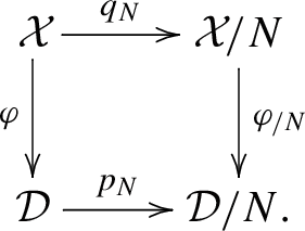  (5.2)

Proof

Consider the quotient mixed Hodge datum $q_N :(P,\mathcal {X}) \rightarrow (P/N,\mathcal {X}/N)$ defined in (5.1). Any $\overline{h} \in \mathcal {X}/N \subseteq {\text {Hom}}(\mathbb {S}_{\mathbb {C}}, (P/N)_{\mathbb {C}})$ induces a $\mathbb {Q}$-mixed Hodge structure on ${\text {Lie}}(P/N)$, via $\text {Ad}_{P/N} \circ \overline{h} :\mathbb {S}_{\mathbb {C}} \rightarrow (P/N)_{\mathbb {C}} \rightarrow \text {GL}({\text {Lie}}(P/N))_{\mathbb {C}}$, which satisfies the three properties listed in Definition 4.1 with P replaced by P/N and h replaced by $\overline{h}$.

Fix a faithful representation $\overline{\rho } :P/N \rightarrow \text {GL}(V')$ defined over $\mathbb {Q}$. Then the morphism $\overline{\rho } \circ \overline{h}$ induces a $\mathbb {Q}$-mixed Hodge structure on $V'$ by Proposition 2.3 for each $\overline{h} \in \mathcal {X}/N$, and the weight filtration and the Hodge numbers do not depend on the choice of $\overline{h} \in \mathcal {X}/N$. Thus we obtain a map

$$\begin{aligned} \varphi _{/N} :\mathcal {X}/N \rightarrow \{\text {mixed Hodge structures on }V'\}. \end{aligned}$$

Set $\mathcal {D}/N = \varphi _{/N}(\mathcal {X}/N)$. Then we get $\varphi _{/N} :\mathcal {X}/N \rightarrow \mathcal {D}/N$, which by [30, 1.7] is $(P/N)(\mathbb {R})^+(W_{-1}/(W_{-1}\cap N))(\mathbb {C})$-equivariant (here $W_{-1} = \mathcal {R}_u(P)$ and hence $\mathcal {R}_u(P/N) = W_{-1}/(W_{-1}\cap N)$). This establishes (iii) for the space $\mathcal {D}/N$.

By [30, 1.12] the $\mathbb {Q}$-mixed Hodge structures on $V'$ thus obtained are graded-polarized by some collection of non-degenerate bilinear forms (same for all $\overline{h}$). So $\mathcal {D}/N$ is a contained in some classifying space $\mathcal {M}'$. This establishes (i).

Now let us construct the map $p_N :\mathcal {D}\rightarrow \mathcal {D}/N$ and prove properties (ii) and (iv). Take $x \in \mathcal {D}$, and take any $h_x \in \varphi ^{-1}(x)$. Then $\varphi ^{-1}(x) = \exp (F^0_x({\text {Lie}}W_{-1})_{\mathbb {C}}) h_x$ by Lemma 4.2. Note that $\exp (F^0_x({\text {Lie}}W_{-1})_{\mathbb {C}})$ is a subgroup of $P_{\mathbb {C}}$. Then $q_N(\varphi ^{-1}(x)) = q_N(\exp (F^0_x({\text {Lie}}W_{-1})_{\mathbb {C}}) h_x) = \frac{\exp (F^0_x({\text {Lie}}W_{-1})_{\mathbb {C}})}{N(\mathbb {C})\cap \exp (F^0_x({\text {Lie}}W_{-1})_{\mathbb {C}})} q_N(h_x)$.

On the other hand define $\overline{x}:= \varphi _{/N}(q_N(h_x))$. Then $\varphi _{/N}^{-1}(\overline{x}) = \exp (F^0_{\overline{x}}({\text {Lie}}W_{-1}/(W_{-1}\cap N))_{\mathbb {C}}) q_N(h_x)$ again by Lemma 4.2.

We claim that $\frac{\exp (F^0_x({\text {Lie}}W_{-1})_{\mathbb {C}})}{N(\mathbb {C})\cap \exp (F^0_x({\text {Lie}}W_{-1})_{\mathbb {C}})} = \exp (F^0_{\overline{x}}({\text {Lie}}W_{-1}/(W_{-1}\cap N))_{\mathbb {C}})$. Indeed it suffices to check for Lie algebras, i.e. it suffices to prove $F^0_x({\text {Lie}}W_{-1})_{\mathbb {C}}/({\text {Lie}}N_{\mathbb {C}} \cap F^0_x({\text {Lie}}W_{-1})_{\mathbb {C}}) \simeq F^0_{\overline{x}}({\text {Lie}}W_{-1}/(W_{-1}\cap N))_{\mathbb {C}}$ canonically. As $N \lhd P$, we have $\text {Ad}_P({\text {Lie}}N) \subseteq {\text {Lie}}N$. So ${\text {Lie}}N$ is a sub-mixed Hodge structure of the adjoint Hodge structure on ${\text {Lie}}P$. Thus ${\text {Lie}}N_{\mathbb {C}} \cap F^0_x({\text {Lie}}W_{-1})_{\mathbb {C}} = F^0_x({\text {Lie}}W_{-1}\cap N)_{\mathbb {C}}$. Thus we proved the desired claim.

By the last three paragraphs, we have $q_N(\varphi ^{-1}(x)) = \varphi _{/N}^{-1}(\overline{x})$. So the map $\mathcal {D}\rightarrow \mathcal {D}/N$, $x \mapsto \overline{x}:=\varphi _{/N}(q_N(h_x))$ is well-defined. Call this map $p_N$. Then property (iv) holds true by construction of $p_N$. Property (ii) then is not hard to check.

Now the map is complex analytic by property (ii). $\square$

6 Fibered structure and real points

Let $\mathcal {D}$ be a Mumford–Tate domain in some classifying space $\mathcal {M}$ with $P = \text {MT}(\mathcal {D})$. Let the connected mixed Hodge datum $(P,\mathcal {X})$ and the $P(\mathbb {R})^+W_{-1}(\mathbb {C})^+$-equivariant map $\varphi :\mathcal {X}\rightarrow \mathcal {D}$ be as in Proposition 4.4.(i). In particular by Lemma 4.2, the fiber $\varphi ^{-1}(x)$ is a principal homogeneous space under $\exp (F^0_x({\text {Lie}}W_{-1})_{\mathbb {C}})$ for each $x \in \mathcal {D}$.

6.1 Fibered structure of Mumford–Tate domains

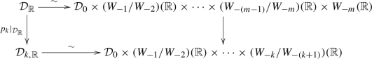
Let $0 = W_{-(m+1)} \subseteq W_{-m} \subseteq \cdots \subseteq W_{-1}$ be the sequence of unipotent normal subgroups of P defined in (B.1).

First for each $k \in \{0,\ldots ,m\}$, let $\mathcal {X}_k = \mathcal {X}/W_{-(k+1)}$ and let

$$\begin{aligned} p_k :\mathcal {D}\rightarrow \mathcal {D}/W_{-(k+1)} =: \mathcal {D}_k \end{aligned}$$

(6.1)

be the quotient constructed in Proposition 5.1. Notice that $\mathcal {X}_m = \mathcal {X}$ and $p_m$ is the identity on $\mathcal {D}$.

Observe that we have $(P/W_{-k},\mathcal {X}_k) = (P/W_{-(k+1)},\mathcal {X}_{k+1})/(W_{-(k+1)}/W_{-(k+2)})$ and $\mathcal {D}_k = \mathcal {D}_{k+1}/(W_{-(k+1)}/W_{-(k+2)})$. Denote by $q_{k+1,k} :(P/W_{-(k+1)},\mathcal {X}_{k+1}) \rightarrow (P/W_{-k},\mathcal {X}_k)$ and $p_{k+1,k} :\mathcal {D}_{k+1} \rightarrow \mathcal {D}_k$ the quotients. Then by Proposition 5.1 we have the following commutative diagram

(6.2)

By Lemma 4.2, $\varphi _0$ is bijective. But the other $\varphi _i$’s are not injective in general.

Let $k \in \{0,\ldots , m-1\}$. Recall that $W_{-(k+1)}/W_{-(k+2)} = {\text {Lie}}W_{-(k+1)}/ W_{-(k+2)}$ is a vector group. Thus for any $x_k \in \mathcal {D}_{k}$, the notation $F^0_{x_k}(W_{-(k+1)}/W_{-(k+2)})_{\mathbb {C}}$ makes sense.

Lemma 6.1

For each $k \in \{0,\ldots , m\}$ and any point $x_k \in \mathcal {D}_k$, we have that

• (i) the fiber $\varphi _k^{-1}(x_k)$ is a principal homogeneous space under $F^0_{x_k}(W_{-(k+1)}/W_{-(k+2)})_{\mathbb {C}}$.

• (ii) (for $k \le m-1$) the fiber $p_{k+1,k}^{-1}(x_k)$ is a principal homogeneous space under

  $$\begin{aligned} (W_{-(k+1)}/W_{-(k+2)})(\mathbb {C}) / F^0_{x_k}(W_{-(k+1)}/W_{-(k+2)})_{\mathbb {C}}. \end{aligned}$$

Proof

Part (i) follows directly from Lemma 4.2.

For (ii): By [30, 1.8(a)], each fiber of $q_{k+1,k}$ is a principal homogeneous space under $(W_{-(k+1)}/W_{-(k+2)})(\mathbb {C})$. Combined with part (i) we can conclude. $\square$

6.2 Real points

Define $\mathcal {D}_{\mathbb {R}}$ to be the set of $x \in \mathcal {D}$ such that the mixed Hodge structure parametrized by x is split over $\mathbb {R}$. Namely, $\mathcal {D}_{\mathbb {R}} = \varphi (\mathcal {X}_{\mathbb {R}})$ with $\mathcal {X}_{\mathbb {R}} = \{ h :\mathbb {S}_{\mathbb {C}} \rightarrow P_{\mathbb {C}}: h\text { is defined over }\mathbb {R}\} \subseteq \mathcal {X}$.

It is known that $\mathcal {D}_{\mathbb {R}} = P(\mathbb {R})^+x$ for some $x \in \mathcal {D}$; see [28, last Remark of Sect. 3].

Moreover for any $x \in \mathcal {D}_{\mathbb {R}}$, it is not hard to check that $F^0_x({\text {Lie}}W_{-1})_{\mathbb {C}} \cap {\text {Lie}}P_{\mathbb {R}} = \{0\}$. So by Lemma 4.2, $p_0 :P \rightarrow G = P/W_{-1}$ induces

$$\begin{aligned} \text {Stab}_{P(\mathbb {R})^+}(x) \simeq \text {Stab}_{G(\mathbb {R})^+}(p_0(x)). \end{aligned}$$

(6.3)

Consider the real semi-algebraic $P(\mathbb {R})^+$-equivariant retraction induced by the $\mathfrak {sl}_2$-splitting [5, Thm. 2.18] (see also [3, Cor. 3.12])

$$\begin{aligned} r :\mathcal {D}\rightarrow \mathcal {D}_{\mathbb {R}}. \end{aligned}$$

(6.4)

For each $k \in \{0,\ldots ,m-1\}$, $\mathcal {D}_k$ is a Mumford–Tate domain and hence we can define $\mathcal {D}_{k,\mathbb {R}}$ as above. Then $\mathcal {D}_{k,\mathbb {R}}$ is a $(P/W_{-(k+1)})(\mathbb {R})^+$-orbit, and there is a real semi-algebraic $(P/W_{-(k+1)})(\mathbb {R})^+$-equivariant retraction $r_k :\mathcal {D}_k \rightarrow \mathcal {D}_{k,\mathbb {R}}$ induced by the $\mathfrak {sl}_2$-splitting.

Let $p_k :\mathcal {D}\rightarrow \mathcal {D}_k$ be from (6.1). The following diagram is commutative by [3, Lem. 6.6]:

(6.5)

We close this subsection with the following proposition, which states that $\mathcal {D}_{\mathbb {R}}$ can be split (non-canonically) into the product of a Mumford–Tate domain for pure Hodge structures and some vector spaces.

Proposition 6.2

There exists a real algebraic isomorphism

$$\begin{aligned} \mathcal {D}_{\mathbb {R}} \simeq \mathcal {D}_{0} \times (W_{-1}/W_{-2})(\mathbb {R}) \times \cdots \times (W_{-(m-1)}/W_{-m})(\mathbb {R}) \times W_{-m}(\mathbb {R}) \end{aligned}$$

(6.6)

with the following properties.

• (i) For any $g = (g_0, w_1,\ldots , w_m) \in P(\mathbb {R})^+$ under the identification (B.6) and any $x = (x_0,x_1,\ldots ,x_m) \in \mathcal {D}_{\mathbb {R}}$ under (6.6), the action of $P(\mathbb {R})^+$ on $\mathcal {D}_{\mathbb {R}}$ is given by the formula

  $$\begin{aligned} gx= & {} (g_0 x_0, w_1 + g_0 x_1, w_2+g_0 x_2 + \text {calb}_2(w_1, g_0 x_1), \ldots ,\nonumber \\ {}{} & {} w_m + g_0 x_m + \text {calb}_m(\textbf{w}_{m-1}, g_0\textbf{x}_{m-1})) \end{aligned}$$

  (6.7)

  where $\textbf{w}_k = (w_1,\ldots , w_k)$ and $\textbf{x}_k = (x_1,\ldots ,x_k)$ for all $k \ge 1$, and the $\text {calb}_k$’s are the $\mathbb {Q}$-polynomials of degree at most $k-1$ given by Lemma B.3.

• (ii) The decomposition (6.6) is compatible with taking quotients of $W_{-(k+1)}$ on both sides for each $k \in \{0,\ldots ,m-1\}$, i.e., the following diagram commutes

  

  where the top arrow is (6.6), the bottom arrow is (6.6) applied to $\mathcal {D}_{k,\mathbb {R}}$, and the right arrow is omitting the last $m-k$ factors.

Proof

First note that $\mathcal {D}_{0,\mathbb {R}} = \mathcal {D}_0$ because every pure Hodge structure is split over $\mathbb {R}$. Now (B.6) and (6.3) together induce a real algebraic isomorphism as in (6.6). Part (ii) is clear. Part (i) follows from the group law given by (B.7). $\square$

7 Period Map and Logarithmic Ax

7.1 Period map

Let S be an irreducible algebraic variety defined over $\mathbb {C}$. Assume that S carries a graded-polarized VMHS $(\mathbb {V}_\mathbb {Z},W_\bullet ,\mathcal {F}^\bullet ) \rightarrow S$. Then it induces a period map $[\Phi ] :S \rightarrow \Gamma \backslash \mathcal {M}$ where $\mathcal {M}$ is the classifying space and $\Gamma$ is an arithmetic subgroup of $P^{\mathcal {M}}(\mathbb {Q})$.

The period map $[\Phi ]$ factors through another quotient space in the following way. In the context of Theorem 1.1, we have a complex analytic irreducible subset $\mathcal {Z}$ of $S \times _{\Gamma \backslash \mathcal {M}}\mathcal {M}= \{(s,x) \in S \times \mathcal {M}: [\Phi ](s) = u(x)\}$, where $u :\mathcal {M}\rightarrow \Gamma \backslash \mathcal {M}$. For the projection $p_{\mathcal {M}} :S\times \mathcal {M}\rightarrow \mathcal {M}$, we have that $p_{\mathcal {M}}(\mathcal {Z})$ is irreducible and is contained in $u^{-1}([\Phi ](S))$. Let $\widetilde{S}$ be a complex analytic irreducible component of $u^{-1}([\Phi ](S))$ which contains $p_{\mathcal {M}}(\mathcal {Z})$. Then $\mathcal {Z} \subseteq S \times \widetilde{S}$. Let $\mathcal {D}= \widetilde{S}^{\text {sp}}$, the smallest Mumford–Tate domain containing $\widetilde{S}$; see Corollary 2.8. Let $P = \text {MT}(\widetilde{S})$ and $W_{-1} = \mathcal {R}_u(P)$, then $\mathcal {D}$ is a $P(\mathbb {R})^+W_{-1}(\mathbb {C})$-orbit. Now we have $[\Phi ](S) \subseteq u(\mathcal {D})$.

Let $\Gamma _P = \Gamma \cap P(\mathbb {Q})$, then $[\Phi ]$ factors through $S \rightarrow \Gamma _P \backslash \mathcal {D}$. The inclusion $\mathcal {D}\subseteq \mathcal {M}$ induces a finite map $\Gamma _P \backslash \mathcal {D}\rightarrow \Gamma \backslash \mathcal {M}$.

Let $\Delta = S \times _{\Gamma _P\backslash \mathcal {D}}\mathcal {D}$. So to prove Theorem 1.1, it suffices to work in the following diagram and assume $\mathcal {Z} \subseteq \Delta$

(7.1)

This is our setup for the rest of the paper.

7.2 Quotient for the period map

Assume $N \lhd P$. We have constructed the quotient Mumford–Tate domain $p_N :\mathcal {D}\rightarrow \mathcal {D}/N$ in Proposition 5.1. For the arithmetic group $\Gamma _{P/N}:= \Gamma _P/(\Gamma _P \cap N(\mathbb {Q}))$, we then have a map $[p_N] :\Gamma _P \backslash \mathcal {D}\rightarrow \Gamma _{P/N}\backslash (\mathcal {D}/N)$. Composing with $[\Phi ] :S \rightarrow \Gamma _P \backslash \mathcal {D}$, we obtain

$$\begin{aligned}{}[\Phi _{/N}] :S \rightarrow \Gamma _{P/N}\backslash (\mathcal {D}/N). \end{aligned}$$

(7.2)

Proposition 5.1 says that $\mathcal {D}/N$ is a Mumford–Tate domain in the classifying space of some mixed Hodge structures. Thus $[\Phi _{/N}]$ is again a period map.

Let us summarize the notations involving this operation of taking quotient in the following diagram:

(7.3)

7.3 Bi-algebraic system

Recall that $\mathcal {M}$ is a semi-algebraic open subset in some algebraic variety $\mathcal {M}^\vee$ over $\mathbb {C}$. So $\mathcal {D}$ is a semi-algebraic open subset in some algebraic variety $\mathcal {D}^\vee$ over $\mathbb {C}$.

Definition 7.1

• (i) A subset of $\mathcal {D}$ is said to be irreducible algebraic if it is a complex analytic irreducible component of $U \cap \mathcal {D}$, with U an algebraic subvariety of $\mathcal {D}^\vee$.

• (ii) An irreducible algebraic subset W of $\mathcal {D}$ is said to be bi-algebraic if $[\Phi ]^{-1}(u(W))$ is algebraic.

By [3, Cor. 6.7], every weak Mumford–Tate domain is bi-algebraic.

7.4 Logarithmic Ax

In this subsection, we prove a particular case of Theorem 1.1. Retain $\mathcal {Z}$ as in Theorem 1.1 and the notations in and above (7.3). As discussed before, we have $\mathcal {Z} \subseteq \Delta \cap (S \times \widetilde{S})$.

Theorem 7.2

There is a smallest weak Mumford–Tate domain in $\mathcal {D}$, denoted by $\widetilde{S}^{\text {ws}}$, which contains $\widetilde{S}$. Moreover,

• (i) $\mathcal {Z}^{\text {Zar}} \subseteq S \times \widetilde{S}^{\text {ws}}$.

• (ii) Theorem 1.1 holds if $u_S(\mathcal {Z}) = S$.

In the proof, we will see that $\widetilde{S}^{\text {ws}}$ is an $N(\mathbb {R})^+(W_{-1}\cap N)(\mathbb {C})$-orbit, where N is the connected algebraic monodromy group of $(\mathbb {V},W_\bullet ,\mathcal {F}^{\bullet }) \rightarrow S$.

Proof

Let N be the connected algebraic monodromy group of $(\mathbb {V},W_{\bullet },\mathcal {F}^{\bullet }) \rightarrow S$. Then $N \lhd P$ by Theorem 3.4. Thus $N(\mathbb {R})^+(W_{-1}\cap N)(\mathbb {C})\widetilde{s}$ is a weak Mumford–Tate domain, for any $\widetilde{s} \in \widetilde{S}$.

As $N \lhd P$, we have the quotient period map $[\Phi _{/N}] :S \rightarrow \Gamma _{S/N}\backslash (\mathcal {D}/N)$ constructed in (7.2). Note that $[\Phi _{/N}]$ gives rise to a new VMHS over S, whose connected algebraic monodromy group is trivial. So $[\Phi _{/N}](S)$ is a point by [8, Thm. 7.12]. Thus using the notations in (7.3), we have that $p_N(\widetilde{S})$ is a point. So $\widetilde{S} \subseteq N(\mathbb {R})^+(W_{-1}\cap N)(\mathbb {C})\widetilde{s}$ for any $\widetilde{s} \in \widetilde{S}$.

In particular $N(\mathbb {R})^+(W_{-1}\cap N)(\mathbb {C})\widetilde{s}$ is independent of the choice of $\widetilde{s} \in \widetilde{S}$.

Let us start by proving part (ii). In the course of this proof, we will also show the existence of $\widetilde{S}^{\text {ws}}$.

Assume $u_S(\mathcal {Z}) = S$. Since $\mathcal {Z} \subseteq S \times \widetilde{S}$, the following is true: For each $s \in S$, there exists $\widetilde{s} \in \widetilde{S}$ such that $(s,\widetilde{s}) \in \mathcal {Z}$.

The group $P(\mathbb {R})^+W_{-1}(\mathbb {C})$ acts on $S \times \mathcal {D}$ via its action on the second factor. Let $\rho :\pi _1(S,s) \rightarrow \text {GL}(V)$ be the monodromy representation. Then $\text {Im}(\rho )$ is a subgroup of $\Gamma _P$. By construction of $\widetilde{S}$, we have $\text {Im}(\rho )(s,\widetilde{s}) \subseteq \mathcal {Z}$ for any $(s,\widetilde{s}) \in \mathcal {Z}$. Taking Zariski closures of both sides and recalling that $N = (\text {Im}(\rho )^{\text {Zar}})^{\circ }$, we have $\{s\} \times N(\mathbb {R})^+(W_{-1}\cap N)(\mathbb {C})\widetilde{s} \subseteq \mathcal {Z}^{\text {Zar}}$. As this holds true for each $s \in S$, we then have $S \times N(\mathbb {R})^+(W_{-1}\cap N)(\mathbb {C})\widetilde{s} \subseteq \mathcal {Z}^{\text {Zar}}$.

To sum it up, we have $\mathcal {Z} \subseteq S \times \widetilde{S} \subseteq S \times N(\mathbb {R})^+(W_{-1}\cap N)(\mathbb {C})\widetilde{s} \subseteq \mathcal {Z}^{\text {Zar}}$. By taking Zariski closures, we have $\mathcal {Z}^{\text {Zar}} = S \times N(\mathbb {R})^+(W_{-1}\cap N)(\mathbb {C})\widetilde{s}$ and $\widetilde{S}^{\text {Zar}} = N(\mathbb {R})^+(W_{-1}\cap N)(\mathbb {C})\widetilde{s}$.

By definition, $N(\mathbb {R})^+(W_{-1}\cap N)(\mathbb {C})\widetilde{s}$ is a weak Mumford–Tate domain. Moreover if $\mathcal {W}$ is a weak Mumford–Tate domain which contains $\widetilde{S}$, then $\mathcal {W}$ contains $\widetilde{S}^{\text {Zar}} = N(\mathbb {R})^+(W_{-1}\cap N)(\mathbb {C})\widetilde{s}$ because $\mathcal {W}$ is algebraic. So $N(\mathbb {R})^+(W_{-1}\cap N)(\mathbb {C})\widetilde{s}$ is the smallest weak Mumford–Tate domain which contains $\widetilde{S}$. Thus $\widetilde{S}^{\text {ws}}$ exists and is precisely $N(\mathbb {R})^+(W_{-1}\cap N)(\mathbb {C})\widetilde{s}$. Now part (ii) is established.

Now part (i) is immediately true because $\mathcal {Z} \subseteq S \times \widetilde{S}$ and $S \times \widetilde{S}^{\text {ws}}$ is algebraic. $\square$

Remark 7.3

If we assume $S = u_S(\mathcal {Z})^{\text {Zar}}$, then $\widetilde{S}^{\text {ws}}$ is the smallest weak Mumford–Tate domain which contains $p_{\mathcal {D}}(\mathcal {Z})$. Indeed, we have $p_{\mathcal {D}}(\mathcal {Z}) \subseteq \widetilde{S}^{\text {ws}}$ by Theorem 7.2.(i). So it suffices to prove the following statement: for any W a weak Mumford–Tate domain in $\mathcal {D}$ which contains $p_{\mathcal {D}}(\mathcal {Z})$, we have $\widetilde{S}^{\text {ws}} \subseteq W$. This is true: $u(W) \supseteq u(p_{\mathcal {D}}(\mathcal {Z})) = [\Phi ](u_S(\mathcal {Z}))$, so $[\Phi ]^{-1}(u(W)) \supseteq u_S(\mathcal {Z})$, so $[\Phi ]^{-1}(u(W)) \supseteq S$ because $[\Phi ]^{-1}(u(W))$ is algebraic (by [3, Cor. 6.7]) and $S = u_S(\mathcal {Z})^{\text {Zar}}$. Therefore $\widetilde{S}^{\text {ws}} \subseteq W$ and hence we are done.

8 Dévissage and Preparation

In this section, we do some preparations. Recall the setup (7.1)

Lemma 8.1

If Theorem 1.1 holds true under the following two additional assumptions:

• (i) $S = u_S(\mathcal {Z})^{\text {Zar}}$.

• (ii) $\mathcal {Z}$ is a complex analytic irreducible component of $\mathcal {Z}^{\text {Zar}} \cap \Delta$.

then it holds true in full generality.

Proof

Let $\mathcal {Z}$ be as in Theorem 1.1. Notice that $\mathcal {Z}^{\text {Zar}} \subseteq u_S(\mathcal {Z})^{\text {Zar}} \times \mathcal {D}$. The assumptions and the conclusion of Theorem 1.1 do not change if we replace S by $u_S(\mathcal {Z})^{\text {Zar}}$. So we may assume $S = u_S(\mathcal {Z})^{\text {Zar}}$.

Let $\mathcal {Z}'$ be a complex analytic irreducible component of $\mathcal {Z}^{\text {Zar}} \cap \Delta$ which contains $\mathcal {Z}$. Note that $\mathcal {Z} \subseteq \mathcal {Z}' \subseteq \mathcal {Z}^{\text {Zar}}$. Thus by taking the Zariski closures, we obtain $\mathcal {Z}'^{\text {Zar}} = \mathcal {Z}^{\text {Zar}}$.

Thus $p_{\mathcal {D}}(\mathcal {Z}'^{\text {Zar}}) = p_{\mathcal {D}}(\mathcal {Z}^{\text {Zar}})$, for the projection $p_{\mathcal {D}} :S \times \mathcal {D}\rightarrow \mathcal {D}$. So for the algebraic structure on $\mathcal {D}$ defined by Definition 7.1, we have $p_{\mathcal {D}}(\mathcal {Z}')^{\text {Zar}} = p_{\mathcal {D}}(\mathcal {Z})^{\text {Zar}}$ because the projection $p_{\mathcal {D}}$ is algebraic. But each weak Mumford–Tate domain is algebraic. So

$$\begin{aligned} p_{\mathcal {D}}(\mathcal {Z}') \subseteq p_{\mathcal {D}}(\mathcal {Z}')^{\text {Zar}} = p_{\mathcal {D}}(\mathcal {Z})^{\text {Zar}} \subseteq p_{\mathcal {D}}(\mathcal {Z})^{\text {ws}} = \widetilde{S}^{\text {ws}}, \end{aligned}$$

where the last equality follows from Remark 7.3. But $p_{\mathcal {D}}(\mathcal {Z}) \subseteq p_{\mathcal {D}}(\mathcal {Z}')$ because $\mathcal {Z} \subseteq \mathcal {Z}'$. So every weak Mumford–Tate domain containing $p_{\mathcal {D}}(\mathcal {Z}')$ must also contain $p_{\mathcal {D}}(\mathcal {Z})$, and thus contains $\widetilde{S}^{\text {ws}}$ by Remark 7.3. Combined with the inclusion above, we get that $\widetilde{S}^{\text {ws}}$ is also the smallest weak Mumford–Tate domain which contains $p_{\mathcal {D}}(\mathcal {Z}')$. So

$$\begin{aligned} \dim \mathcal {Z}^{'\text {Zar}} - \dim \mathcal {Z}' \ge \dim p_{\mathcal {D}}(\mathcal {Z}')^{\text {ws}} \Longrightarrow \dim \mathcal {Z}^{\text {Zar}} - \dim \mathcal {Z} \ge \dim p_{\mathcal {D}}(\mathcal {Z})^{\text {ws}} \end{aligned}$$

as $\dim \mathcal {Z} \le \dim \mathcal {Z}'$ and $p_{\mathcal {D}}(\mathcal {Z})^{\text {ws}} = p_{\mathcal {D}}(\mathcal {Z}')^{\text {ws}} = \widetilde{S}^{\text {ws}}$. Replacing $\mathcal {Z}$ by $\mathcal {Z}'$, it is thus enough to prove Theorem 1.1 assuming furthermore (ii). $\square$

Thus our main theorem is reduced to the following theorem, which we will prove in the rest of the paper.

Theorem 8.2

Theorem 1.1 holds true under the additionnal assumption that $\mathcal {Z}$ is a complex analytic irreducible component of $\mathcal {Z}^{\text {Zar}} \cap \Delta$ and $S = u_S(\mathcal {Z})^{\text {Zar}}$.

The rest of the paper is devoted to prove Theorem 8.2.

9 Bigness of the $\mathbb {Q}$-stabilizer

Recall our setup

(9.1)

We consider a subset $\mathcal {Z}$ of $\Delta$ satisfying the following properties: (i) $\mathcal {Z}$ is a complex analytic irreducible component of $\mathcal {Z}^{\text {Zar}}\cap \Delta$; (ii) $S = u_S(\mathcal {Z})^{\text {Zar}}$.

Let $H_{\mathcal {Z}^{\text {Zar}}}$ be the $\mathbb {Q}$-stabilizer of $\mathcal {Z}^\text {Zar}$, namely

$$\begin{aligned} H_{\mathcal {Z}^{\text {Zar}}} = \left( \text {Stab}_{P(\mathbb {R})}(\mathcal {Z}^{\text {Zar}}) \cap \Gamma _P \right) ^{\text {Zar},\circ } = \left( \{\gamma \in \Gamma _P: \gamma \mathcal {Z}^{\text {Zar}} = \mathcal {Z}^{\text {Zar}}\}^{\text {Zar}}\right) ^{\circ }. \end{aligned}$$

(9.2)

In this section, we prove the following case of Theorem 8.2:

Proposition 9.1

Theorem 8.2 holds true under the additional assumption $H_{\mathcal {Z}^{\text {Zar}}}$ is the trivial group.

9.1 Auxiliary set

Our proof of Proposition 9.1 heavily uses o-minimality. We are able to work in this framework thanks to the following theorem proved by the second-named author, Bakker, Brunebarbe, and Tsimerman. In the pure case this theorem is the main result of [4].

Theorem 9.2

[3, Prop. 3.13 and Thm. 4.4] Let $r :\mathcal {D}\rightarrow \mathcal {D}_{\mathbb {R}}$ be the retraction defined in (6.4), and identify $\mathcal {D}_{\mathbb {R}}$ with $\mathcal {D}_0 \times \prod _{1\le k \le m} (W_{-k}/W_{-k-1})(\mathbb {R})$ under the real-algebraic isomorphism defined in (6.6).

There exist an $\mathbb {R}_{\text {alg}}$-definable subset $\mathfrak {F}_0$ of $\mathcal {D}_0$ and a real number $M > 0$ such that

$$\begin{aligned} \mathfrak {F}_{\mathbb {R}}:= \mathfrak {F}_0 \times \prod _{1 \le k \le m} (-M,M)^{\dim (W_{-k}/W_{-(k+1)})(\mathbb {R})}, \end{aligned}$$

(9.3)

which is a $\mathbb {R}_{\text {alg}}$-definable subset of $\mathcal {D}_{\mathbb {R}}$, satisfies the following properties:

• (i) $u|_{r^{-1}(\mathfrak {F}_{\mathbb {R}})}$ is surjective;

• (ii) $[\Phi ]$ is $\mathbb {R}_{\text {an},\exp }$-definable for the $\mathbb {R}_{\text {alg}}$-structure on $\Gamma _P\backslash \mathcal {D}$ defined by $r^{-1}(\mathfrak {F}_{\mathbb {R}})$.

The following auxiliary set is important for the proof of Ax–Schanuel.

$$\begin{aligned} \Theta := \{g \in P(\mathbb {R}): \dim (g^{-1} \mathcal {Z}^{\text {Zar}} \cap (S \times \mathfrak {F}) \cap \Delta ) = \dim \mathcal {Z} \}, \end{aligned}$$

(9.4)

with $\mathfrak {F} = r^{-1}(\mathfrak {F}_{\mathbb {R}})$. It is clear that $\Theta$ is definable in $\mathbb {R}_{\text {an},\exp }$, and

$$\begin{aligned} \{\gamma \in \Gamma _P: \gamma (S\times \mathfrak {F}) \cap \mathcal {Z} \not = \emptyset \} \subseteq \Theta . \end{aligned}$$

Denote for simplicity by $\widetilde{Z} = p_{\mathcal {D}}(\mathcal {Z})$, then

$$\begin{aligned} p_{\mathcal {D}}\left( \gamma (S\times \mathfrak {F}) \cap \mathcal {Z} \right) = p_{\mathcal {D}}(p_{\mathcal {D}}^{-1}(\gamma \mathfrak {F}) \cap \mathcal {Z}) = \gamma \mathfrak {F} \cap \widetilde{Z}. \end{aligned}$$

Thus for any $\gamma \in \Gamma _P$, we have

$$\begin{aligned} \gamma (S\times \mathfrak {F}) \cap \mathcal {Z} \not =\emptyset \Leftrightarrow \gamma \mathfrak {F} \cap \widetilde{Z} \not =\emptyset . \end{aligned}$$

Therefore

$$\begin{aligned} \{\gamma \in \Gamma _P: \gamma \mathfrak {F} \cap \widetilde{Z} \not = \emptyset \} \subseteq \Theta . \end{aligned}$$

(9.5)

Theorem 9.3

Assume $\dim \widetilde{Z} > 0$. Then there exist constants $\epsilon > 0$, $c_{\epsilon }>0$ and a sequence of real numbers $\{T_i\}_{i\in \mathbb {N}}$ with $T_i \rightarrow \infty$ such that

$$\begin{aligned} \#\{\gamma \in \Theta \cap \Gamma _P: H(\gamma ) \le T_i\} \ge c_{\epsilon } T_i^{\epsilon }. \end{aligned}$$

(9.6)

9.2 Proof of Proposition 9.1 assuming Theorem 9.3

If $\dim \widetilde{Z} = 0$, then $\dim \widetilde{Z}^{\text {ws}} = 0$ and hence Theorem 8.2 clearly holds true. So we assume $\dim \widetilde{Z} > 0$.

We prove Proposition 9.1 by (downward) induction on $\dim \mathcal {Z}^{\text {Zar}}$. The starting point for this induction is when $\mathcal {Z}^{\text {Zar}} = S \times \widetilde{S}^{\text {ws}}$ (see Theorem 7.2). In this case, under the assumptions of Theorem 8.2 we have $\mathcal {Z} = S\times _{\Gamma _P\backslash \mathcal {D}} \widetilde{S}^{\text {ws}}$, and so $\dim \mathcal {Z} = \dim S$. Thus Theorem 8.2 holds true in this case.

Let $c_{\epsilon }>0$, $\epsilon >0$ and $\{T_i\}$ be as in Theorem 9.3. Then by the Pila–Wilkie counting theorem [29, 3.6], for each $T_i$ there exists a connected semi-algebraic curve $C_i \subseteq \Theta$ which contains $\ge c_{\epsilon }T_i^{\epsilon }$ points in $\Gamma _P$ of height at most $T_i$. For $T_i \gg 1$ we have $c_{\epsilon }T_i^{\epsilon } \ge 2$.

Fix $c_0 \in C_i \cap \Gamma _P$. Set $C:= c_0^{-1} \cdot C_i$. Then C is a semi-algebraic curve which contains $\ge c_{\epsilon }T_i^{\epsilon }$ in $\Gamma _P$.

For each $c' \in C_i \subseteq \Theta$, we have $\dim (c^{\prime -1}\mathcal {Z}^{\text {Zar}} \cap \Delta ) = \dim \mathcal {Z}$ by definition of $\Theta$ from (9.4). But $c_0 \Delta = \Delta$ since $c_0 \in \Gamma _P$. So we have

$$\begin{aligned} \dim (c^{-1}\mathcal {Z}^{\text {Zar}} \cap \Delta ) = \dim \mathcal {Z}\qquad \text { for all }c \in C. \end{aligned}$$

(9.7)

Notice that $\mathcal {Z}^{\text {Zar}} \subseteq C^{-1}\mathcal {Z}^{\text {Zar}}$. Moroever since C is a semi-algebraic curve, we have $\dim (C^{-1}\mathcal {Z}^{\text {Zar}})^{\text {Zar}} \le \dim \mathcal {Z}^{\text {Zar}} + 1$.

We have the following alternative:

• (i) $\dim (C^{-1}\mathcal {Z}^{\text {Zar}})^{\text {Zar}} = \dim \mathcal {Z}^{\text {Zar}}$;

• (ii) $\dim (C^{-1}\mathcal {Z}^{\text {Zar}})^{\text {Zar}} = \dim \mathcal {Z}^{\text {Zar}}+1$.

Assume we are in case (i). Then $C \subseteq \text {Stab}_{P(\mathbb {R})}(\mathcal {Z}^{\text {Zar}})$. Hence $\#(\text {Stab}_{P(\mathbb {R})}(\mathcal {Z}^{\text {Zar}}) \cap \Gamma _P) \ge C \cap \Gamma _P \ge c_{\epsilon }T_i^{\epsilon }$ for each i. Letting $T_i \rightarrow \infty$, we get $\#(\text {Stab}_{P(\mathbb {R})}(\mathcal {Z}^{\text {Zar}}) \cap \Gamma ) = \infty$. Hence $\dim H_{\mathcal {Z}^{\text {Zar}}} > 0$. This contradicts the triviality of $H_{\mathcal {Z}^{\text {Zar}}}$.

Thus we are in case (ii). Then there exists $c \in C$ such that $\mathcal {Z}^{\text {Zar}} \not = c^{-1}\mathcal {Z}^{\text {Zar}}$. Thus $\mathcal {Z} \not \subseteq c^{-1}\mathcal {Z}^{\text {Zar}}$; otherwise taking the Zariski closures we get $\mathcal {Z}^{\text {Zar}} \subseteq c^{-1}\mathcal {Z}^{\text {Zar}}$, hence $\mathcal {Z}^{\text {Zar}} = c^{-1}\mathcal {Z}^{\text {Zar}}$ by comparing dimensions, contradicting the choice of c. Thus $c^{-1}\mathcal {Z}^{\text {Zar}} \cap \Delta$ varies with $c \in C$. Therefore by (9.7), an irreducible component $\mathcal {Z}' \supseteq \mathcal {Z}$ of $(C^{-1}\mathcal {Z}^{\text {Zar}})^{\text {Zar}} \cap \Delta$ which has dimension $\ge \dim \mathcal {Z} + 1$.

We claim that $\mathcal {Z}^{\prime \text {Zar}} = (C^{-1}\mathcal {Z}^{\text {Zar}})^{\text {Zar}}$. Indeed, otherwise $\mathcal {Z}^{\prime \text {Zar}} = \mathcal {Z}^{\text {Zar}}$ by dimension comparisons. But then the assumption of Theorem 8.2 says that $\mathcal {Z}$ is a component of $\mathcal {Z}^{\text {Zar}} \cap \Delta = \mathcal {Z}^{\prime \text {Zar}}\cap \Delta$. Hence $\mathcal {Z}' \subseteq \mathcal {Z}$. This contradicts $\dim \mathcal {Z}' \ge \dim \mathcal {Z}+1$.

So we can apply the induction hypothesis to $\mathcal {Z}'$ and obtain

$$\begin{aligned} \dim \mathcal {Z}^{\prime \text {Zar}} - \dim \mathcal {Z}' \ge \dim p_{\mathcal {D}}(\mathcal {Z}')^{\text {ws}}. \end{aligned}$$

But the left hand side $\le \dim \mathcal {Z}^{\text {Zar}} - \dim \mathcal {Z}$ and the right hand side is $\ge \dim p_{\mathcal {D}}(\mathcal {Z})^{\text {ws}}$. Hence Theorem 8.2 holds true for $\mathcal {Z}$.

We are done.

9.3 Preparation of the proof of Theorem 9.3

We will prove Theorem 9.3, or more precisely (9.6), in the rest of this section. The proof is long. It will be divided in several steps for readers’ convenience. In this subsection, we fix some notations.

The proof of (9.6) uses the fibered structure of $\mathcal {D}$ and the discussion on its real points, both explained in Sect. 6. We start by recollecting basic knowledge on both aspects.

Recall the sequence of normal subgroups

$$\begin{aligned} 0 = W_{-(m+1)} \subseteq W_{-m} \subseteq \cdots W_{-1} = \mathcal {R}_u(P) \end{aligned}$$

of P from (B.1), and the quotient Mumford–Tate domains $p_k :\mathcal {D}\rightarrow \mathcal {D}_k:= \mathcal {D}/W_{-k-1}$, for each $k \in \{0,\ldots ,m\}$, from (6.1). Notice that $p_m$ is the identity map on $\mathcal {D}$.

Let $r :\mathcal {D}\rightarrow \mathcal {D}_{\mathbb {R}}$ be the $P(\mathbb {R})^+$-equivariant retraction of the inclusion $\mathcal {D}_{\mathbb {R}}\subseteq \mathcal {D}$ from (6.4). Applying (6.5) successively to $p_{k,k-1} :\mathcal {D}_{k+1} \rightarrow \mathcal {D}_k$ (defined in the diagram (6.2)), we obtain the following commutative diagram

(9.8)

with each $r_k$ a $(P/W_{-k-1})(\mathbb {R})^+$-equivariant retraction of $\mathcal {D}_{k,\mathbb {R}} \subseteq \mathcal {D}_k$. Recall that $\mathcal {D}_{0}$ is a Mumford–Tate domain in a classifying space of pure Hodge structures, and $r_0$ is the identity map. There is a metric on $\mathcal {D}_0$; see [6, beginning of Sect. 2.1].

In the proof, we often need to project subsets of $\mathcal {D}$ to different levels and consider the real points. So it is convenient to fix the following notations.

Notation 9.4

For each $k \in \{0,1,\cdots ,m\}$,

• For any subset $A \subseteq \mathcal {D}$, denote by $A_k:= p_k(A) \subseteq \mathcal {D}_{k}$. As convention $A_m = A$.

• For any subset $A \subseteq \mathcal {D}$, denote by $A_{\mathbb {R}}:= r(A) \subseteq \mathcal {D}_{\mathbb {R}}$, and $A_{k,\mathbb {R}} = r_k(A_k) \subseteq \mathcal {D}_{k,\mathbb {R}}$.

Let $\mathfrak {F} = r^{-1}(\mathfrak {F}_{\mathbb {R}})$ where $\mathfrak {F}_{\mathbb {R}} \subseteq \mathcal {D}_{\mathbb {R}}$ is given by Theorem 9.2, or more precisely by (9.3).

Before moving on, let us sketch how (9.6) is proved when $m = 0$, namely when $\mathcal {D}= \mathcal {D}_0$ and $P = P/W_{-1}$ is a reductive group. In this case, $\widetilde{Z} = \widetilde{Z}_0$, which has positive dimension by assumption. For each real number $T > 0$, take $\textbf{B}_0(T) \subseteq \mathcal {D}_{0}$ to be the ball centered at a fixed point of radius $\log T$ in $\mathcal {D}_{0}$. Let $\widetilde{Z}_0(T)$ be a complex analytic irreducible component of $\widetilde{Z} \cap \textbf{B}_0(T)$. The following estimate is a direct corollary of Thm. 1.2 and Thm. 4.2 of Bakker–Tsimerman [6]: There exist constants $c_0, \epsilon _0 > 0$, independent of T, such that

$$\begin{aligned} \#\{\gamma \in \Gamma _P: \gamma \mathfrak {F} \cap \widetilde{Z}_0(T) \not = \emptyset , ~ H(\gamma ) \le T \} \ge c_0 T^{\epsilon _0}. \end{aligned}$$

See also [7, Prop. 6.3] for the statement of this estimate. By (9.5), the set on the left hand side is a subset of $\#\{\gamma \in \Theta \cap \Gamma _P: H(\gamma ) \le T\}$. This yields (9.6).

For a general m, we need to generalize this idea. A first thing to do is to find an appropriate generalization of $\textbf{B}_0(T)$ for $\mathcal {D}$. To achieve this, we make use of the retractions $r_k$’s (with $r_m = r$) and the following product structure on $\mathcal {D}_{\mathbb {R}}$ (6.6) (and the truncated version given by Proposition 6.2.(ii) for each $k \in \{0,1,\cdots ,m\}$)

$$\begin{aligned} \mathcal {D}_{k,\mathbb {R}} \simeq \mathcal {D}_{0,\mathbb {R}} \times (W_{-1}/W_{-2})(\mathbb {R}) \times (W_{-2}/W_{-3})(\mathbb {R}) \times \cdots \times (W_{-k}/W_{-k-1})(\mathbb {R}).\nonumber \\ \end{aligned}$$

(9.9)

Now we are ready to give the generalization of the $\textbf{B}_0(T)$ above. For each $k \in \{0,1,\cdots ,m\}$ and each real number $T > 0$, define the following subset $\textbf{B}_k(T) \subseteq \mathcal {D}_k$ as follows.

• Let $\textbf{B}_0(T) = B_0(T) \subseteq \mathcal {D}_{0}$ be the ball of radius $\log T$ centered at a fixed point in $\widetilde{Z}_0$.

• For each $k \ge 1$, let $B_k(T)$ the $| \cdot |$-ball centered at 0 of radius T in $(W_{-k}/W_{-k-1})(\mathbb {R})$, i.e. $B_k(T) = \{w \in (W_{-k}/W_{-k-1})(\mathbb {R}): |w| < T\}$. Define $\textbf{B}_k(T) = r_k^{-1}(\prod _{i=0}^k B_i(T))$. In particular, $p_{k+1,k}(\textbf{B}_{k+1}(T)) = \textbf{B}_k(T)$, and $\textbf{B}_k(T)_{\mathbb {R}} = \prod _{i=0}^k B_i(T)$.

Next, we need to generalize the set $\widetilde{Z}_0(T)$. For each $k \ge 0$:

• Let $\widetilde{Z}_k(T)$ be a complex analytic irreducible component of $\widetilde{Z}_k \cap \textbf{B}_k(T) \subseteq \mathcal {D}_k$.

• We may choose such $\widetilde{Z}_k(T)$’s that $p_{k+1,k} (\widetilde{Z}_{k+1}(T)) \subseteq \widetilde{Z}_k(T)$ for all k.²

Finally for the purpose of lifting, we need to introduce the following sets, which generalize the set $\widetilde{Z}(T)$ from [19, proof of Thm. 5.2] (which handles the case where $m=1$). Let $k_0$ be such that $\dim \widetilde{Z}_{k_0} > 0$, smallest for this property. For each $k \in \{k_0+1,\cdots ,m\}$ and each real number $T > 0$ (the diagram (9.10) below, with k replaced by $k-1$, is helpful to keep track of the notation):

• Let $\widetilde{Z}(k,T):= \widetilde{Z}_k \cap p_{k,k-1}^{-1}(\widetilde{Z}_{k-1}(T)) \subseteq \mathcal {D}_k$, and $\widetilde{Z}(k,T)^+$ be a complex analytic irreducible component of $\widetilde{Z}(k,T)$.

• Similar to the $\widetilde{Z}_k(T)$’s, we may choose such $\widetilde{Z}(k,T)^+$’s that $p_{k+1,k} (\widetilde{Z}(k+1,T)^+) \subseteq \widetilde{Z}(k,T)^+$ for all k.

Notice that by definition, we have $p_{k,k-1}(\widetilde{Z}(k,T)) = \widetilde{Z}_{k-1} \cap \widetilde{Z}_{k-1}(T) = \widetilde{Z}_{k-1}(T) \subseteq \widetilde{Z}_{k-1} \cap \textbf{B}_{k-1}(T)$.

9.4 Sketch of the strategy of the proof of Theorem 9.3

For simplicity, we use the same notation $p_k$ to denote the projection $P \rightarrow P/W_{-k-1}$ and the projection $\mathcal {D}\rightarrow \mathcal {D}_k$. In the proof we need to work with many subscripts, and the following diagram is helpful to keep track of them.

(9.10)

where the real-algebraic isomorphism $\mathcal {D}_{k+1,\mathbb {R}} \simeq \mathcal {D}_{k,\mathbb {R}} \times (W_{-k-1}/W_{-k-2})(\mathbb {R})$ is from (9.9). Notice that $\widetilde{Z}(k+1,T)_{\mathbb {R}}$ is a component of $\widetilde{Z}_{k+1,\mathbb {R}} \bigcap (\prod _{i=0}^k B_i(T) \times (W_{-k-1}/W_{-k-2})(\mathbb {R}))$, and that $\widetilde{Z}_k(T)_{\mathbb {R}}$ is a component of $\widetilde{Z}_{k,\mathbb {R}} \bigcap \prod _{i=0}^k B_i(T)$.

Suppose $\dim \widetilde{Z}_0 = \dim p_0(\widetilde{Z}) > 0$. By the results of Bakker and Tsimerman as explained above, we find $\#\{\gamma _0 \in p_0(\Gamma _P): \gamma _0 \mathfrak {F}_0 \cap \widetilde{Z}_0(T) \not = \emptyset , ~ H(\gamma _0) \le T \} \ge c_0T^{\epsilon _0}$. Consider the diagram (9.10) with $k=0$. We wish to lift at least polynomially many such $\gamma _0$’s to elements in $p_1(\Gamma _P)$ of height at most T with the following property: each such lift $\gamma _1 \in p_1(\Gamma _P)$ satisfies $\gamma _1\mathfrak {F}_1 \cap \widetilde{Z}(1,T) \not = \emptyset$, or equivalently $\gamma _1 r_1(\mathfrak {F}_1) \cap r_1(\widetilde{Z}(1,T)) \not =\emptyset$ (since $\mathfrak {F}_1 = r_1^{-1}(\mathfrak {F}_{1,\mathbb {R}})$ by definition of $\mathfrak {F}$). This last condition, expressed with Notation 9.4, becomes $\gamma _1 \mathfrak {F}_{1,\mathbb {R}}\cap \widetilde{Z}(1,T)_{\mathbb {R}} \not =\emptyset$. The intersection is taken in $\mathcal {D}_{1,\mathbb {R}} \simeq \mathcal {D}_0 \times (W_{-1}/W_{-2})(\mathbb {R})$. If the desired lifting can be realized, then we do similar liftings to $p_2(\Gamma _P)$, etc., under we obtain at least polynomially many elements $\gamma$ in $p_m(\Gamma _P) = \Gamma _P$ of height at most T such that $\gamma \mathfrak {F}_{\mathbb {R}} \cap \widetilde{Z}(T)_{\mathbb {R}} \not = \emptyset$.

At this stage, we can explain why the second bullet point in the constructions of the $\widetilde{Z}(k,T)$’s is needed: in the lifting process, we need that $\widetilde{Z}(k+1,T)_{\mathbb {R}}$ is mapped into $\widetilde{Z}(k,T)_{\mathbb {R}}$ under $p_{k+1,k}$.

There is a problem in the procedure described above, namely it is possible that $\widetilde{Z}_0$ is a point. In this case, we need to work with the smallest $k_0$ such that $\dim \widetilde{Z}_{k_0} > 0$, which serves as the base step of the lifting process. Thus we need to introduce the set $\widetilde{Z}_{k_0}(T)$, which is a complex analytic irreducible component of $\widetilde{Z}_{k_0} \cap \textbf{B}_{k_0}(T)$. We need to find at least polynomially many elements $\gamma _{k_0} \in p_{k_0}(\Gamma _P)$ of height at most T such that $\gamma _{k_0} \mathfrak {F}_{k_0,\mathbb {R}} \cap \widetilde{Z}_{k_0}(T)_{\mathbb {R}} \not = \emptyset$. Whereas this is guaranteed by the result of Bakker and Tsimerman when $k_0 = 0$, it is not known when $k_0 \ge 1$. We will prove this result in Sect. 9.5, or more precisely Proposition 9.5.(ii).

Once we have established the base step, we need to realize the lifting. In view of (9.10), in order to realize the lifting process from k to $k+1$, we need to compare the growth of $\widetilde{Z}(k+1,T)_{\mathbb {R}} \subseteq \mathcal {D}_{k+1,\mathbb {R}}$ in the vertical direction $(W_{-k-1}/W_{-k-2})(\mathbb {R})$ with its growth in the horizontal direction $\mathcal {D}_{k,\mathbb {R}}$. This lifting process is done in Sect. 9.8. As in [19, proof of Thm. 5.2], we will divide into the two cases where $\widetilde{Z}(k+1,T)_{\mathbb {R}}$ grows “faster” in the vertical direction $(W_{-k-1}/W_{-k-2})(\mathbb {R})$ (Lemma 9.11) and where $\widetilde{Z}(k+1,T)_{\mathbb {R}}$ grows “faster” in the horizontal direction $\mathcal {D}_{k,\mathbb {R}}$ (the rest of Sect. 9.8).

9.5 Proof of Theorem 9.3: the base step

The main goal of this subsection is to prove the base step for the lifting process, namely Proposition 9.5. At the end of this subsection we also state the result for the lifting process (Proposition 9.10) and explain how it implies Theorem 9.3. The proof of the lifting process will be executed in the next subsection.

Let $k_0 \in \{0,\cdots ,m\}$ be such that $\dim \widetilde{Z}_{k_0} > 0$, smallest for this property. For simplicity, we introduce the following notation. For each real number $T \ge 0$, let

$$\begin{aligned} \Xi _{k_0}(T)&:= \{g \in (W_{-k_0}/W_{-k_0-1})(\mathbb {R}) : g \mathfrak {F}_{k_0} \cap \widetilde{Z}_{k_0}(T) \not =\emptyset \} \nonumber \\&= \{g \in (W_{-k_0}/W_{-k_0-1})(\mathbb {R}) : g \mathfrak {F}_{k_0,\mathbb {R}} \cap \widetilde{Z}_{k_0}(T)_{\mathbb {R}} \not =\emptyset \}. \end{aligned}$$

(9.11)

Here the second equality holds true since $\mathfrak {F}_{k_0} = r_{k_0}^{-1}( \mathfrak {F}_{k_0,\mathbb {R}})$.

We also denote by $\Gamma _{-k_0/-k_0-1} = (\Gamma _P \cap W_{-k_0}(\mathbb {Q})) / (\Gamma _P \cap W_{-k_0-1}(\mathbb {Q}))$; it is a subgroup of $P/W_{-k_0-1}$ and acts on $\mathcal {D}_{k_0} = \mathcal {D}/W_{-k_0-1}$.

Proposition 9.5

There exist constants $c_{k_0}, \epsilon _{k_0} > 0$ such that

$$\begin{aligned} \#\{\gamma _{-k_0/-k_0-1} \!\in \! \Xi _{k_0}(T) \cap \Gamma _{-k_0/-k_0-1}: H(\gamma _{-k_0/-k_0-1}) \!\le \! T \} \!\ge \! c_{k_0} T^{\epsilon _{k_0}}\quad \! \text {for all }T \!\gg \! 1. \end{aligned}$$

Proof of Proposition 9.5

If $k_0 = 0$, this is proved in [6]. We refer to [7, Prop. 6.3] for a precise statement.

From now on, assume $k_0 \ge 1$. We use (9.10) with $k = k_0-1$. Now $\widetilde{Z}_{k_0-1} = \overline{h}$ is a point in $\mathcal {D}_{k_0-1}$. Thus $\widetilde{Z}_{k_0} \subseteq p_{k_0,k_0-1}^{-1}(\overline{h})$. Notice that $r_{k_0}(p_{k_0,k_0-1}^{-1}(\overline{h}))$ can be identified with $(W_{-k_0}/W_{-k_0-1})(\mathbb {R})$.

Lemma 9.6

Recall $M > 0$ the real number in the definition of $\mathfrak {F}_{\mathbb {R}}$ from Theorem 9.2. Denote for simplicity $\mathfrak {F}'_{k_0} = (-M,M)^{\dim (W_{-k_0}/W_{-k_0-1})(\mathbb {R})} \subseteq (W_{-k_0}/W_{-k_0-1})(\mathbb {R})$. Then any $\gamma _{-k_0/-k_0-1} \in \Xi _{k_0}(T) \cap \Gamma _{-k_0/-k_0-1}$ satisfies $H(\gamma _{-k_0/-k_0-1}) \le T+M$.

Proof of Lemma 9.6

We have $\widetilde{Z}_{k_0,\mathbb {R}} = r_{k_0}(\widetilde{Z}_{k_0}) \subseteq r_{k_0}(p_{k_0,k_0-1}^{-1}(\overline{h})) = (W_{-k_0}/W_{-k_0-1})(\mathbb {R})$. Recall the definition $\textbf{B}_{k_0}(T) = r_{k_0}^{-1}(\prod _{i=0}^{k_0} B_i(T))$. So

$$\begin{aligned}{} & {} \Xi _{k_0}(T) \cap \Gamma _{-k_0/-k_0-1} = \{\gamma _{-k_0/-k_0-1} \in \Gamma _{-k_0/-k_0-1}:\nonumber \\{} & {} \left( \gamma _{-k_0/-k_0-1} + \mathfrak {F}'_{k_0} \right) \cap \widetilde{Z}_{k_0}(T)_{\mathbb {R}} \not = \emptyset \}. \end{aligned}$$

(9.12)

Hence each $\gamma _{-k_0/-k_0-1} \in \Xi _{k_0}(T) \cap \Gamma _{-k_0/-k_0-1}$ satisfies $\left( \gamma _{-k_0/-k_0-1} + \mathfrak {F}'_{k_0} \right) \cap B_{k_0}(T)_{\mathbb {R}} \not = \emptyset$. We are done. $\square$

Now we are ready to finish the proof of Proposition 9.5.

Consider $\{\gamma _{-k_0/-k_0-1} \in \Gamma _{-k_0/-k_0-1}: (\gamma _{-k_0/-k_0-1} + \mathfrak {F}'_{k_0}) \cap \widetilde{Z}_{k_0,\mathbb {R}} \not = \emptyset \}$. We claim that it is infinite. Indeed, assume otherwise, then $\widetilde{Z}_{k_0,\mathbb {R}}$ is contained in a bounded subset of $(W_{-k_0}/W_{-k_0-1})(\mathbb {R})$. But $p_{k_0,k_0-1}^{-1}(\overline{h}) \simeq (W_{-k_0}/W_{-k_0-1})(\mathbb {C})/F^0_{\overline{h}}(W_{-k_0}/W_{-k_0-1})_{\mathbb {C}}$ by part (ii) of Lemma 6.1, and the composite ($\varphi _{k_0}$ is the natural projection)

$$\begin{aligned} (W_{-k_0}/W_{-k_0-1})(\mathbb {C})&\xrightarrow {\varphi _{k_0}} (W_{-k_0}/W_{-k_0-1})(\mathbb {C}) / F^0_{\overline{h}}(W_{-k_0}/W_{-k_0-1})_{\mathbb {C}} = p_{k_0,k_0-1}^{-1}(\overline{h}) \nonumber \\&\xrightarrow {r_{k_0}} (W_{-k_0}/W_{-k_0-1})(\mathbb {R}) \end{aligned}$$

(9.13)

is, up to an automorphism of $(W_{-k_0}/W_{-k_0-1})(\mathbb {R})$ sending bounded sets to bounded sets, the projection to the real part.³ So $\varphi _{k_0}^{-1}(\widetilde{Z}_{k_0}) \subseteq \varphi _{k_0}^{-1}(r_{k_0}^{-1}(\widetilde{Z}_{k_0,\mathbb {R}}))$ is contained in a set whose real part is bounded. But $\varphi _{k_0}^{-1}(\widetilde{Z}_{k_0})$ is complex analytic, so $\varphi _{k_0}^{-1}(\widetilde{Z}_{k_0})$ is a point, and so is $\widetilde{Z}_{k_0}$. This contradicts $\dim \widetilde{Z}_{k_0} > 0$.

Next we claim that $\widetilde{Z}_{k_0}(T)_{\mathbb {R}}$ passes through the boundary of $B_{k_0}(T)$. Assume otherwise, then $\widetilde{Z}_{k_0,\mathbb {R}} {\setminus } \widetilde{Z}_{k_0}(T)_{\mathbb {R}}$ and $\widetilde{Z}_{k_0}(T)_{\mathbb {R}}$ are disjoint. But $\widetilde{Z}_{k_0,\mathbb {R}}$ is connected since $\widetilde{Z}_{k_0}$ is irreducible. So we must have $\widetilde{Z}_{k_0,\mathbb {R}} = \widetilde{Z}_{k_0}(T)_{\mathbb {R}}$. Hence $\widetilde{Z}_{k_0,\mathbb {R}}$ is contained in a bounded subset of $(W_{-k_0}/W_{-k_0-1})(\mathbb {R})$. This yields a contradiction by the same argument in the previous paragraph.

Note that $\mathfrak {F}'_{k_0}$ is a fundamental set for the action of $\Gamma _{-k_0/-k_0-1}$ on the Euclidean space $(W_{-k_0}/W_{-k_0-1})(\mathbb {R})$. The claims in the previous two paragraphs together immediately imply that

$$\begin{aligned} \#\{\gamma _{-k_0/-k_0-1} \in \Gamma _{-k_0/-k_0-1}: (\gamma _{-k_0/-k_0-1} + \mathfrak {F}'_{k_0}) \cap \widetilde{Z}_{k_0}(T)_{\mathbb {R}} \not = \emptyset \} \ge T \end{aligned}$$

for all $T \gg 1$. Now the conclusion follows from Lemma 9.6 with $c_{k_0} =1/2$ and $\epsilon _{k_0} = 1$. $\square$

Remark 9.7

The proof of Proposition 9.5 is the only place in the proof of Theorem 9.3 where we use the complex structure of $\mathcal {D}$. More precisely, the complex structure of $\mathcal {D}$ is used only in the citation of [6] (if $k_0 = 0$) and in the paragraph involving (9.13) (if $k_0 \ge 1$).

9.6 A preliminary lifting process

Let $k \ge 0$. For simplicity denote by $W_0:= P$. The following diagram is useful to keep track of the notations.

(9.14)

where the real-algebraic isomorphism $\mathcal {D}_{k+1,\mathbb {R}} \simeq \mathcal {D}_{k,\mathbb {R}} \times (W_{-k-1}/W_{-k-2})(\mathbb {R})$ is from (9.9), and $\lambda _{k+1}$ is the natural projection.

Consider the isomorphism of $\mathbb {Q}$-varieties given by (B.6) $P/W_{-k-2} \simeq G \times (W_{-1}/W_{-2}) \times \cdots \times (W_{-k-1}/W_{-k-2})$. It induces

$$\begin{aligned} P/W_{-k-2} \simeq P/W_{-k-1} \times W_{-k-1/-k-2}. \end{aligned}$$

(9.15)

The group $(P/W_{-k-2})(\mathbb {R})^+$ acts on $\mathcal {D}_{k+1,\mathbb {R}} = (\mathcal {D}/W_{-k-2})_{\mathbb {R}}$. Write

$$\begin{aligned} \Gamma _{0/-k-2} = \Gamma _P/(\Gamma _P \cap W_{-k-2}(\mathbb {Q})). \end{aligned}$$

Lemma 9.8

There exists a constant $\beta _k > 0$ with the following property. Consider the Euclidean norm $| \cdot |$ on $(W_{-k-1}/W_{-k-2})(\mathbb {R})$. Then for any $\gamma _{0/-k-2} \in \Gamma _{0/-k-2}$, the set $\lambda _{k+1}(\gamma _{0/-k-2} \mathfrak {F}_{k+1,\mathbb {R}})$ is contained in a $|\cdot |$-ball of radius $\le \beta _k H(\gamma _{0/-k-1})^{k}$ in $(W_{-k-1}/W_{-k-2})(\mathbb {R})$. Here, $\gamma _{0/-k-1} \in \Gamma _{0/-k-1}$ is the projection of $\gamma _{0/-k-2}$ under the natural projection $P/W_{-k-2} \rightarrow P/W_{-k-1}$.

Moreover, if we denote by $(\gamma _{0/-k-1}, \gamma _{-k-1/-k-2})$ the image of $\gamma _{0/-k-2}$ under the isomorphism (9.15), then the $|\cdot |$-ball mentioned above can be taken to be centered at $\gamma _{-k-1/-k-2}$.

Before proving Lemma 9.8, let us see an application.

Lemma 9.9

There exist constants $\alpha _k >0$ and $\alpha '_k > 0$ satisfying the following property. If $\gamma _{0/-k-1} \in \Gamma _{0/-k-1}$ satisfies $\gamma _{0/-k-1} \mathfrak {F}_{k,\mathbb {R}} \cap \prod _{i=0}^{k} B_i(T) \not = \emptyset$, then $H(\gamma _{0/-k-1}) \le \alpha '_k T^{\alpha _k}$.

Proof of Lemma 9.9

We prove this lemma by upward induction on $k \ge 0$. The base step is $k = 0$, which is precisely [6, Thm. 4.2].

Use the notation from (9.14).

Assume Lemma 9.9 holds true for k, namely $H(\gamma _{0/-k-1}) \le \alpha '_k T^{\alpha _k}$ for each $\gamma _{0/-k-1} \in \Gamma _{0/-k-1}$ with $\gamma _{0/-k-1} \mathfrak {F}_{k,\mathbb {R}} \cap \prod _{i=0}^{k} B_i(T) \not = \emptyset$. We wish to prove the property for $k+1$.

Let $\gamma _{0/-k-2} \in \Gamma _{0/-k-2}$ be such that $\gamma _{0/-k-2} \mathfrak {F}_{k+1,\mathbb {R}} \cap \prod _{i=0}^{k+1} B_i(T) \not = \emptyset$. Denote by $(\gamma _{0/-k-1},\gamma _{-k-1/-k-2})$ the image of $\gamma _{0/-k-2}$ under the isomorphism (9.15). In particular, $\gamma _{0/-k-1}$ is the image of $\gamma _{0/-k-2}$ under the projection $p_{k+1,k} :P/W_{-k-2} \rightarrow P/W_{-k-1}$.

Applying $p_{k+1,k}$ to both sides of $\gamma _{0/-k-2} \mathfrak {F}_{k+1,\mathbb {R}} \cap \prod _{i=0}^{k+1} B_i(T) \not = \emptyset$, we obtain that $\gamma _{0/-k-1} \mathfrak {F}_{k,\mathbb {R}} \cap \prod _{i=0}^{k} B_i(T) \not = \emptyset$. Thus by induction hypothesis, we have $H(\gamma _{0/-k-1}) \le \alpha '_k T^{\alpha _k}$.

Next, applying $\lambda _{k+1}$ to both sides of $\gamma _{0/-k-2} \mathfrak {F}_{k+1,\mathbb {R}} \cap \prod _{i=0}^{k+1} B_i(T) \not =\emptyset$, we then have

$$\begin{aligned} \lambda _{k+1}(\gamma _{0/-k-2} \mathfrak {F}_{k+1,\mathbb {R}}) \cap B_{k+1}(T) \not =\emptyset . \end{aligned}$$

(9.16)

By Lemma 9.8, $\lambda _{k+1}(\gamma _{0/-k-2} \mathfrak {F}_{k+1,\mathbb {R}})$ is contained in a $|\cdot |$-ball of radius $\beta _k H(\gamma _{0/-k-1})^{k}$ centered at $\gamma _{-k-1/-k-2}$. But $H(\gamma _{0/-k-1}) \le \alpha '_k T^{\alpha _k}$. Therefore the following two $|\cdot |$-balls in the Euclidean space $(W_{-k-1}/W_{-k-2})(\mathbb {R})$ intersect: the one of radius T centered at 0, and the one of radius $\beta _k \alpha _k^{\prime k} T^{k \alpha _k}$ centered at $\gamma _{-k-1/-k-2}$. So $H(\gamma _{-k-1/-k-2}) \le T+\beta _k \alpha _k^{\prime k} T^{k \alpha _k}$.

Thus the proposition holds true with $\alpha '_{k+1}:= 1+\beta _k \alpha _k^{\prime k}$ and $\alpha _{k+1} = \max \{1,k\alpha _k\}$. $\square$

We end this subsection with:

Proof of Lemma 9.8

Let $\gamma _{0/-k-2} \in \Gamma _{0/-k-2}$. Use the notation as in the lemma, namely $\gamma _{0/-k-2} \mapsto (\gamma _{0/-k-1}, \gamma _{-k-1/-k-2})$ under the isomorphism of $\mathbb {Q}$-varieties $P/W_{-k-2} \simeq P/W_{-k-1} \times (W_{-k-1}/W_{-k-2})$ (9.15).

Next, consider the isomorphism of $\mathbb {Q}$-varieties induced by (B.6)

$$\begin{aligned} P/W_{-k-2} \simeq G \times (W_{-1}/W_{-2}) \times \cdots \times (W_{-k-1}/W_{-k-2}), \end{aligned}$$

and suppose $\gamma _{0/-k-2} \mapsto (\gamma _{0/-1}, \gamma _{-1/-2}, \ldots , \gamma _{-k-1/-k-2})$ under this isomorphism. Then $H(\gamma _{0/-k-2}) = \max \{H(\gamma _{0/-1}), \ldots , H(\gamma _{-k-1/-k-2})\}$.

On the other hand, for the real-algebraic morphism induced by (9.9)

$$\begin{aligned} \mathcal {D}_{k+1,\mathbb {R}}\simeq & {} \mathcal {D}_0 \times (W_{-1}/W_{-2})(\mathbb {R}) \times \cdots \\{} & {} \times (W_{-k-1}/W_{-k-2})(\mathbb {R}) \times (W_{-k-1}/W_{-k-2})(\mathbb {R}), \end{aligned}$$

we have defined, in (9.3), $\mathfrak {F}_{k+1,\mathbb {R}}$ to be the inverse image of $\mathfrak {F}_0 \times \mathfrak {F}'_1 \times \cdots \times \mathfrak {F}'_{k+1}$, where M is a fixed real number and

$$\begin{aligned} \mathfrak {F}'_i = (-M,M)^{\dim (W_{-i}/W_{-i-1})(\mathbb {R})} \subseteq (W_{-i}/W_{-i-1})(\mathbb {R}). \end{aligned}$$

The formula for the action of the group $(P/W_{-k-2})(\mathbb {R})^+$ on $\mathcal {D}_{k+1,\mathbb {R}}$ is given by Proposition 6.2, or more precisely (6.7). Thus

$$\begin{aligned}&\lambda _{k+1}(\gamma _{0/-k-2} \mathfrak {F}_{k+1,\mathbb {R}}) \nonumber \\&\quad = \{ \gamma _{-k-1/-k-2} + \gamma _{0/-1} \widetilde{x} + \text {calb}_{k+1}(\gamma _{0/-k-1} , \gamma _{0/-1} \widetilde{x}'):\nonumber \\&\qquad \quad \widetilde{x} \in \mathfrak {F}'_{k+1}, ~ \widetilde{x}' \in \mathfrak {F}_0 \times \mathfrak {F}'_1 \times \cdots \times \mathfrak {F}'_{k}\} \nonumber \\&\quad = \gamma _{-k-1/-k-2} + \gamma _{0/-1} \cdot \mathfrak {F}'_{k+1}\nonumber \\&\qquad +\text {calb}_{k+1}(\gamma _{0/-k-1}, \gamma _{0/-1} \mathfrak {F}_0 \times \gamma _{0/-1} \mathfrak {F}'_1 \times \cdots \times \gamma _{0/-1} \mathfrak {F}'_{k} ),\qquad \end{aligned}$$

(9.17)

where $\text {calb}_{k+1}$ is a polynomial of degree at most k. Notice that M, $\mathfrak {F}_0$ and the $\mathfrak {F}'_i$’s are fixed, and that $H(\gamma _{0/-1}) \le H(\gamma _{0/-k-1})$. So

$$\begin{aligned}{} & {} |\gamma _{0/-1} \cdot \mathfrak {F}'_{k+1} + \text {calb}_{k+1}(\gamma _{0/-k-1}, \gamma _{0/-1} (\mathfrak {F}_0 \times \mathfrak {F}'_1 \times \cdots \mathfrak {F}'_{k}) )|\\ {}{} & {} \qquad \ll H(\gamma _{0/-1}) + H(\gamma _{0/-k-1})^{k} \ll H(\gamma _{0/-k-1})^{k}. \end{aligned}$$

Therefore, by (9.17), $\lambda _{k+1}(\gamma _{0/-k-2} \mathfrak {F}_{k+1,\mathbb {R}})$ is contained in the $|\cdot |$-ball of radius $\ll H(\gamma _{0/-k-1})^{k}$ centered at $\gamma _{-k-1/-k-2}$. Hence we are done. $\square$

9.7 Setup and final conclusion of the lifting process

For each $k \in \{k_0, \ldots , m\}$ and each real number $T \ge 0$:

• Let $\Gamma _{-k_0/-k-1} = (\Gamma _P \cap W_{-k_0}(\mathbb {Q}))/(\Gamma _P \cap W_{-k-1}(\mathbb {Q}))$. Then $\Gamma _{-k_0/-k-1}$ acts on $\mathcal {D}_{k} = \mathcal {D}/W_{-k-1}$.

• If furthermore $k \ge k_0+1$, then set

  $$\begin{aligned} \Xi _{k}(T)&= \{g \in (W_{-k_0}/W_{-k-1})(\mathbb {R}) : g \mathfrak {F}_{k} \cap \widetilde{Z}(k,T) \not = \emptyset \} \\&=\{g \in (W_{-k_0}/W_{-k-1})(\mathbb {R}) : g \mathfrak {F}_{k,\mathbb {R}} \cap \widetilde{Z}(k,T)_{\mathbb {R}} \not = \emptyset \} \subseteq (P/W_{-k-1})(\mathbb {R}), \end{aligned}$$

  where the second equality follows from the construction $\mathfrak {F}_k = r_k^{-1}(\mathfrak {F}_{k,\mathbb {R}})$.

Notice that the above definition of $\Xi _k(T)$ for $k \ge k_0+1$ differs in an essential way from the definition for $\Xi _{k_0}(T)$ given in (9.11), because for $\Xi _{k_0}(T)$ we intersect with $\widetilde{Z}_{k_0}(T)$ while in case $k \ge k_0+1$ the intersection is with $\widetilde{Z}(k,T)_{\mathbb {R}}$ (which is larger than $\widetilde{Z}_k(T)_{\mathbb {R}}$). This seemingly strange convention will make the induction step of the proof of Proposition 9.10 much cleaner.

Now we are ready to state the desired lifting proposition.

Proposition 9.10

For each $k \ge k_0$, there exist constants $c_k, \epsilon _k> 0$, and a sequence $\{T_i \in \mathbb {R}\}_{i \in \mathbb {N}}$ with $T_i \rightarrow \infty$, such that

$$\begin{aligned} \#\{\gamma _{-k_0/-k-1} \in \Xi _{k}(T_i) \cap \Gamma _{-k_0/-k-1}: H(\gamma _{-k_0/-k-1}) \le T_i \} \ge c_k T_i^{\epsilon _k}. \end{aligned}$$

Let us finish the proof of Theorem 9.3 assuming this proposition.

Proof of Theorem 9.3 assuming Proposition 9.10

Apply Proposition 9.10 to $k = m$. As $W_{-(m+1)} = 0$, the conclusion of the proposition becomes: there exist constants $c=c_m, \epsilon =\epsilon _m > 0$ and a sequence $\{T_i \in \mathbb {R}\}_{i \in \mathbb {N}}$ with $T_i \rightarrow \infty$, such that

$$\begin{aligned} \#\{\gamma \in \Gamma _{-k}: H(\gamma ) \le T_i, ~ \gamma \mathfrak {F} \cap \widetilde{Z}(m,T_i) \not = \emptyset \} \ge c T_i^{\epsilon }. \end{aligned}$$

But $\Gamma _{-k_0} \subseteq \Gamma _P$ and $\widetilde{Z}(m,T_i) \subseteq \widetilde{Z}$, and so

$$\begin{aligned} \# \{\gamma \in \Gamma _P: H(\gamma ) \le T_i, ~ \gamma \mathfrak {F} \cap \widetilde{Z} \not = \emptyset \} \ge c T_i^{\epsilon }. \end{aligned}$$

Thus we can conclude by (9.5). $\square$

9.8 Proof of Proposition 9.10

We prove in this subsection Proposition 9.10 with a lifting process. The following diagram helps to keep track of the lifting, with $k \ge k_0$:

(9.18)

where the vertical inclusions are inclusions in the $\mathbb {R}$-points of the underlying groups, and the horizontal inclusions are inclusions in the underlying spaces.

We start with the following observation:

$$\begin{aligned} p_{k+1,k}(\Xi _{k+1}(T)) \subseteq \{g \in (W_{-k}/W_{-k-1})(\mathbb {R}): g \mathfrak {F}_{k,\mathbb {R}} \cap \prod _{i=0}^{k} B_i(T) \not = \emptyset \}.\qquad \end{aligned}$$

(9.19)

Indeed, take $g \in p_{k+1,k}(\Xi _{k+1}(T))$. Then $g = p_{k+1,k}(g')$ for some $g' \in \Xi _{k+1}(T)$. Thus $g' \mathfrak {F}_{k+1,\mathbb {R}}\cap \widetilde{Z}(k+1,T)_{\mathbb {R}} \not =\emptyset$. Applying $p_{k+1,k}$ to both sides, we get $g \mathfrak {F}_{k,\mathbb {R}} \cap p_{k+1,k}(\widetilde{Z}(k+1,T)_{\mathbb {R}}) \not =\emptyset$. But $p_{k+1,k}(\widetilde{Z}(k+1,T)_{\mathbb {R}}) = p_{k+1,k}(r_{k+1}(\widetilde{Z}(k+1,T)) = r_k(p_{k+1,k}(\widetilde{Z}(k+1,T))) \subseteq r_k(\widetilde{Z}_k \cap \textbf{B}_k(T)) \subseteq r_k(\textbf{B}_k(T)) = \prod _{i=0}^{k} B_i(T)$. Hence we get (9.19).

For each $\alpha _k$ from Lemma 9.9, let us fix a number $\delta _k$ such that

$$\begin{aligned} \delta _k > (k+1) \alpha _k. \end{aligned}$$

(9.20)

Now we proceed to the proof. We start with the following lemma, which handles the case where the vertical direction of $\widetilde{Z}(k+1,T_i)$ grows faster than the horizontal direction.

Lemma 9.11

Assume there exists $k \ge k_0$ such that

$$\begin{aligned} |\lambda _{k+1}(\widetilde{Z}(k+1,T)_{\mathbb {R}})| > T^{\delta _k} \qquad \text { for all }T \gg 1. \end{aligned}$$

(9.21)

Then there exist constants $c_{k+1} >0$ and $\epsilon _{k+1} >0$, both independent of T, such that

$$\begin{aligned} \#\{\gamma _{-k_0/-k-2} \in \Xi _{k+1}(T) \cap \Gamma _{-k_0/-k-2}: H(\gamma _{-k_0/-k-2}) \le T\} \ge c_{k+1}T^{\epsilon _{k+1}}.\nonumber \\ \end{aligned}$$

(9.22)

Proof of Lemma 9.11

Use the notation from (9.18). By definition (9.3), we have $\mathfrak {F}_{k+1,\mathbb {R}} = \mathfrak {F}_{k,\mathbb {R}} \times (-M,M)^{\dim (W_{-k-1}/W_{-k-2})(\mathbb {R})}$ for some fixed real number $M>0$.

Take $\gamma _{-k_0/-k-2} \in \Xi _{k+1}(T) \cap \Gamma _{-k_0/-k-2}$. Write $(\gamma _{-k_0/-k-1},\gamma _{-k-1/-k-2})$ for the image of $\gamma _{-k_0/-k-2}$ under the isomorphism (9.15) $P/W_{-k-2} \simeq P/W_{-k-1}\times W_{-k-1/-k-2}$. Then $\gamma _{-k_0/-k-1} = p_{k+1,k}(\gamma _{-k_0/-k-2})$ for the group morphism $p_{k+1,k} :P/W_{-k-2} \rightarrow P/W_{-k-1}$. Thus $H(\gamma _{-k_0/-k-1}) \le \alpha '_k T^{\alpha _k}$ by (9.19) and Lemma 9.9.

We temporarily work in the Euclidean space $(W_{-k-1}/W_{-k-2})(\mathbb {R})$. Our hypothesis (9.21) says that $\lambda _{k+1}(\widetilde{Z}(k+1,T_i)_{\mathbb {R}})$ reaches the boundary of the $|\cdot |$-ball of radius $T_i^{\delta _k}$ centered at 0.

We claim that $\lambda _{k+1}(\widetilde{Z}(k+1,T_i)^+_{\mathbb {R}})$ also reaches the boundary of the $|\cdot |$-ball of radius $T_i^{\delta _k}$ centered at 0 (which by our notation is $B_{k+1}(T_i^{\delta _k})$). Assume otherwise, then $\lambda _{k+1}(\widetilde{Z}_{k+1,\mathbb {R}}) {\setminus } B_{k+1}(T_i^{\delta _k})$ and $\lambda _{k+1}(\widetilde{Z}(k+1,T_i)^+_{\mathbb {R}})$ are disjoint. But $\lambda _{k+1}(\widetilde{Z}_{k+1,\mathbb {R}})$ is connected because $\widetilde{Z}$ is irreducible. So we must have $\lambda _{k+1}(\widetilde{Z}_{k+1,\mathbb {R}}) = \lambda _{k+1}(\widetilde{Z}(k+1,T_i)^+_{\mathbb {R}})$. By definition, we have $\widetilde{Z}(k+1,T)_{\mathbb {R}} \subseteq \widetilde{Z}_{k+1,\mathbb {R}}$. Thus $\lambda _{k+1}(\widetilde{Z}(k+1,T_i)^+_{\mathbb {R}}) = \lambda _{k+1}(\widetilde{Z}_{k+1,\mathbb {R}}) \supseteq \lambda _{k+1}(\widetilde{Z}(k+1,T)_{\mathbb {R}}) \supseteq \lambda _{k+1}(\widetilde{Z}(k+1,T_i)^+_{\mathbb {R}})$, and hence every inclusion is an equality. Now we are done by the assumption (9.21).

On the other hand by Lemma 9.8, the subset $\lambda _{k+1}(\gamma _{-k_0/-k-2}\mathfrak {F}_{k+1,\mathbb {R}} \cap \widetilde{Z}(k+1,T_i)_{\mathbb {R}})$ is contained in a $|\cdot |$-ball of radius $\ll H(\gamma _{-k_0/-k-1})^{k+1} \ll T_i^{(k+1)\alpha _k}$ centered at $\gamma _{-k-1/-k-2}$.

Since $(W_{-k-1}/W_{-k-2})(\mathbb {R})$ is Euclidean and $\delta _k > (k+1)\alpha _k$ and that $\lambda _{k+1}(\widetilde{Z}(k+1,T_i)^+_{\mathbb {R}})$ is connected, the previous two paragraphs together imply

$$\begin{aligned} \#\{\gamma _{-k-1/-k-2} \in&\Gamma _{-k-1/-k-2} : H(\gamma _{-k-1/-k-2}) \le T^{\delta _k}, ~ (\gamma _{-k_0/-k-1}, \gamma _{-k-1/-k-2}) \in \Xi _k(T) \\&\text { for some }\gamma _{-k_0/-k-1} \in p_{k+1,k}(\Xi _{k+1}(T)) \cap \Gamma _{-k_0/-k-1} \} \gg T^{\delta _k - (k+1)\alpha _k} \end{aligned}$$

for all $T\gg 1$. As each $\gamma _{-k_0/-k-1} \in p_{k+1,k}(\Xi _{k+1}(T)) \cap \Gamma _{-k_0/-k-1}$ satisfies $H(\gamma _{-k_0/-k-1}) \le \alpha '_k T^{\alpha _k}$ by (9.19) and Lemma 9.9, the counting above yields, for all $T \gg 1$,

$$\begin{aligned} \#\{(\gamma _{-k_0/-k-1},\gamma _{-k-1/-k-2}) \in \Xi _k(T) \cap \Gamma _{-k_0/-k-2} :&H(\gamma _{-k-1/-k-2}) \le T^{\delta _k}, \\&H(\gamma _{-k_0/-k-2}) \le \alpha '_k T^{\alpha _k} \} \gg T^{\delta _k - (k+1)\alpha _k}. \end{aligned}$$

But the only assumption on $\delta _k$ is $\delta _k > (k+1) \alpha _k$. Hence we have proved (9.22) by choosing appropriately $c_{k+1}$ and $\epsilon _{k+1}$. We are done. $\square$

The next lemma is useful for the lifting in the case where the horizontal direction of $\widetilde{Z}(k+1,T_i)$ grows faster than the vertical direction.

Lemma 9.12

Let $k \ge k_0$. Assume there exists a sequence $\{T_i \in \mathbb {R}\}$, with $T_i \rightarrow \infty$, such that

$$\begin{aligned} |\lambda _{k+1}(\widetilde{Z}(k+1,T_i)_{\mathbb {R}})| \le T_i^{\delta _k}. \end{aligned}$$

(9.23)

Then $H(\gamma _{-k_0/-k-2}) \ll T_i^{\delta _k}$ for each $\gamma _{-k_0/-k-2} \in \Xi _{k+1}(T_i) \cap \Gamma _{-k_0/-k-2}$.

Proof

Use the notation from (9.18).

Take $\gamma _{-k_0/-k-2} \in \Xi _{k+1}(T_i) \cap \Gamma _{-k_0/-k-2}$. Write $(\gamma _{-k_0/-k-1},\gamma _{-k-1/-k-2})$ for the image of $\gamma _{-k_0/-k-2}$ under the isomorphism (9.15) $P/W_{-k-2} \simeq P/W_{-k-1}\times W_{-k-1/-k-2}$. Then $\gamma _{-k_0/-k-1} \in p_{k+1,k}(\Xi _{k+1}(T_i) )$ for the group morphism $p_{k+1,k} :P/W_{-k-2} \rightarrow P/W_{-k-1}$. Thus $H(\gamma _{-k_0/-k-1}) \le \alpha '_k T_i^{\alpha _k}$ by (9.19) and Lemma 9.9.

There exists a point $\widetilde{z}_{k+1} \in \gamma _{-k_0/-k-2} \mathfrak {F}_{k+1,\mathbb {R}} \cap \widetilde{Z}(k+1,T_i)_{\mathbb {R}}$. Write $\widetilde{z}_{k+1,k} = \lambda _{k+1}(\widetilde{z}_{k+1})$.

Now that $\widetilde{z}_{k+1,k}$ is a point in $\lambda _{k+1}(\gamma _{-k_0/-k-2}\mathfrak {F}_{k+1,\mathbb {R}})$, which by Lemma 9.8 is contained in a $|\cdot |$-ball of radius $\le \beta _k H(\gamma _{-k_0/-k-1})^{k+1} \le \beta _k \alpha _k^{\prime k} T_i^{(k+1)\alpha _k}$ centered at $\gamma _{-k-1/-k-2}$. On the other hand $\widetilde{z}_{k+1,k}$ is a point in $\lambda _{k+1}(\widetilde{Z}(k+1,T_i)_{\mathbb {R}})$. So the assumption (9.23) yields $|\widetilde{z}_{k+1,k}| \le T_i^{\delta _k}$. Write $\beta '_k:= \beta _k \alpha _k^{\prime k}$. This says that in the Euclidean space, the following two $|\cdot |$-balls intersect: the one of radius $T_i^{\delta _k}$ centered at 0, and the one of radius $\beta '_k T_i^{(k+1)\alpha _k}$ centered at $\gamma _{-k-1/-k-2}$. Thus we must have $H(\gamma _{-k-1/-k-2}) \le T_i^{\delta _k} + \beta '_k T_i^{(k+1)\alpha _k}$, which furthermore $\le (1+\beta '_k) T_i^{\delta _k}$ by assumption on $\delta _k$.

Therefore $H(\gamma _{-k_0/-k-2}) \le \max \{H(\gamma _{-k_0/-k-1}), H(\gamma _{-k-1/-k-2})\} \ll T_i^{\delta _k}$. $\square$

With these preparations, we are ready to prove Proposition 9.10.

Proof of Proposition 9.10

We prove Proposition 9.10 by induction on $k \ge k_0$.

The base step is $k = k_0$. Recall that in this case, $\Xi _{k_0}(T)$ is defined in a different way than the other $\Xi _k(T)$’s (with $k \ge k_0+1$). Indeed

$$\begin{aligned} \Xi _{k_0}(T):=\{g \in (W_{-k_0}/W_{-k_0-1})(\mathbb {R}): g \mathfrak {F}_{k_0,\mathbb {R}}\cap \widetilde{Z}_{k_0}(T)_{\mathbb {R}}\not =\emptyset \}. \end{aligned}$$

(9.24)

The conclusion for the base step follows immediately from Proposition 9.5, which says: There exist constants $c_{k_0}, \epsilon _{k_0} > 0$ such that

$$\begin{aligned} \#\{\gamma _{-k_0/-k_0-1} \in \Xi _{k_0}(T) \cap \Gamma _{-k_0/-k_0-1}: H(\gamma _{-k_0/-k_0-1}) \le T \} \ge c_{k_0} T^{\epsilon _{k_0}}.\qquad \end{aligned}$$

(9.25)

Assume Proposition 9.10 is proved for $k \ge k_0$, i.e. there exist constants $c_k, \epsilon _k> 0$, and a sequence $\{T_i \in \mathbb {R}\}_{i \in \mathbb {N}}$ with $T_i \rightarrow \infty$, such that

$$\begin{aligned} \#\{\gamma _{-k_0/-k-1} \in \Xi _{k}(T_i) \cap \Gamma _{-k_0/-k-1}: H(\gamma _{-k_0/-k-1}) \le T_i \} \ge c_k T_i^{\epsilon _k}. \end{aligned}$$

(9.26)

We wish to prove for $k+1$, i.e. up to replacing $\{T_i \in \mathbb {R}\}$ by a subsequence, find constants $c_{k+1}, \epsilon _{k+1} > 0$ such that

$$\begin{aligned} \#\{\gamma _{-k_0/-k-2} \in \Xi _{k+1}(T_i) \cap \Gamma _{-k_0/-k-2}: H(\gamma _{-k_0/-k-2}) \le T_i \} \ge c_{k+1} T_i^{\epsilon _{k+1}}.\nonumber \\ \end{aligned}$$

(9.27)

We have two alternatives:

• (i) Either $|\lambda _{k+1}(\widetilde{Z}(k+1,T)_{\mathbb {R}})| > T^{\delta _{k}}$ for all $T \gg 1$,

• (ii) or $|\lambda _{k+1}(\widetilde{Z}(k+1,T_i)_{\mathbb {R}})| \le T_i^{\delta _{k}}$ for some sequence $\{T_i\in \mathbb {R}\}$ with $T_i \rightarrow \infty$.

For case (i), the conclusion follows from Lemma 9.11. So from now on, assume that we are in case (ii).

By Lemma 9.12 we have $H(\gamma _{-k_0/-k-2}) \ll T_i^{\delta _{k}}$ for each $\gamma _{-k_0/-k-2} \in \Xi _{k+1}(T_i) \cap \Gamma _{-k_0/-k-2}$. Thus, to establish (9.27), it suffices to show that $\#(\Xi _{k+1}(T_i) \cap \Gamma _{-k_0/-k-2})$ is at least polynomial in $T_i$.

Notice that

$$\begin{aligned} \widetilde{Z}(k+1,T_i)_{\mathbb {R}} = \bigcup _{\gamma _{-k_0/-k-2}\in \Xi _{k+1}(T_i) \cap \Gamma _{-k_0/-k-2}} \gamma _{-k_0/-k-2}\mathfrak {F}_{k+1,\mathbb {R}} \cap \widetilde{Z}(k+1,T_i)_{\mathbb {R}}. \end{aligned}$$

Applying $p_{k+1,k}|_{\mathcal {D}_{k+1,\mathbb {R}}}$ to both sides, we obtain

$$\begin{aligned} p_{k+1,k}(\widetilde{Z}(k+1,T_i)_{\mathbb {R}}) \subseteq \bigcup _{\gamma _{-k_0/-k-2}\in \Xi _{k+1}(T_i) \cap \Gamma _{-k_0/-k-2}} \gamma _{-k_0/-k-1}\mathfrak {F}_{k,\mathbb {R}}. \end{aligned}$$

Thus $p_{k+1,k}(\widetilde{Z}(k+1,T_i)_{\mathbb {R}})$ hits $\le \#(\Xi _{k+1}(T_i) \cap \Gamma _{-k_0/-k-2})$ fundamental sets which are $\Gamma _{-k_0/-k-1}$-translates of $\mathfrak {F}_{k,\mathbb {R}}$.

On the other hand, we claim that $\widetilde{Z}_k(T_i)_{\mathbb {R}}$ hits at least polynomially fundamental sets which are $\Gamma _{-k_0/-k-1}$-translates of $\mathfrak {F}_{k,\mathbb {R}}$. To show this, we need to divide into two cases: when $k = k_0$ or $k \ge k_0+1$. When $k = k_0$, this follows immediately from (9.25) and the definition of $\Xi _{k_0}(T_i)$ (9.24). It remains to prove the claim for $k \ge k_0+1$. In this case, if $\gamma _{-k_0/-k-1} \in \Xi _{k}(T_i) \cap \Gamma _{-k_0/-k-1}$ with $H(\gamma _{-k_0/-k-1}) \le T_i$, then $\lambda _k(\gamma _{-k_0/-k-1}\mathfrak {F}_{k,\mathbb {R}})$ is contained in a $|\cdot |$-ball of radius $\ll T_i^k$ centered at 0 by Lemma 9.8 (applied with k replaced by $k-1$). Thus $\gamma _{-k_0/-k-1}\mathfrak {F}_{k,\mathbb {R}} \cap \widetilde{Z}_k(T_i^k)_{\mathbb {R}} \not = \emptyset$. So (9.26) yields the claim with $T_i$ replaced by $T_i^k$.

By choice of $\widetilde{Z}(k+1,T_i)$ and $\widetilde{Z}_k(T_i)$, we have that $p_{k+1,k}(\widetilde{Z}(k+1,T)) = \widetilde{Z}_k(T)$; see the end of Sect. 9.3 (or right above Sect. 9.4). Thus $p_{k+1,k}(\widetilde{Z}(k+1,T)_{\mathbb {R}}) = \widetilde{Z}_k(T)_{\mathbb {R}}$. Hence the previous two paragraphs imply that $\#(\Xi _{k+1}(T_i) \cap \Gamma _{-k_0/-k-2})$ is at least polynomial in $T_i$. Hence we are done. $\square$

10 Normality of the $\mathbb {Q}$-stabilizer: Part 1

Let N be the connected algebraic monodromy group of the admissible VMHS $(\mathbb {V}_\mathbb {Z},W_{\bullet },\mathcal {F}^{\bullet })$ on S. Then $N \lhd P$ by Theorem 3.4.

The goal of this section is to prove the following normality result.

Proposition 10.1

$H_{\mathcal {Z}^{\text {Zar}}} \lhd N$.

10.1 Family associated with $\mathcal {Z}$

Let $\textbf{H}$ be the component of the Hilbert scheme of $S \times \mathcal {D}^\vee$ which contains $[\mathcal {Z}^{\text {Zar}}]$, the point representing $\mathcal {Z}^{\text {Zar}}$. Then $\textbf{H}$ is proper. Consider the (modified) universal family

$$\begin{aligned} \textit{B} = \{(x,\widetilde{m}, [\mathcal {B}]) \in (S \times \mathcal {D}) \times \textbf{H}: (x,\widetilde{m}) \in \mathcal {B}\}. \end{aligned}$$

The projection

$$\begin{aligned} \psi :\textit{B} \rightarrow S \times \mathcal {D}\end{aligned}$$

(10.1)

is a proper map since $\textbf{H}$ is proper.

Define

$$\begin{aligned} \textit{Z} = \{(\widetilde{\delta }, [\mathcal {B}]) \in (\Delta \times \textbf{H}) \cap \textit{B}: \dim _{\widetilde{\delta }}(\Delta \cap \mathcal {B}) \ge \dim \mathcal {Z} \}. \end{aligned}$$

Then $\textit{Z}$ is a closed complex analytic subset of $\textit{B}$. So $\psi (\textit{Z})$ is closed complex analytic in $S \times \mathcal {D}$ as $\psi$ is proper. Note that $\psi (\textit{Z}) \subseteq \Delta$.

Let us summarize the notations in the following diagram.

Recall that the arithmetic group $\Gamma _P$ acts on $S \times \mathcal {D}$ by its action on the second factor. We claim that $\Gamma _P \psi (\textit{Z}) = \psi (\textit{Z})$. Indeed, this action of $\Gamma _P$ on $S \times \mathcal {D}$ induces an action of $\Gamma _P$ on $\textit{B}$ by

$$\begin{aligned} \gamma (x,\widetilde{m},[\mathcal {B}]) = (x,\gamma \widetilde{m},[\gamma \mathcal {B}]). \end{aligned}$$

(10.2)

Thus $\Gamma _P \Delta = \Delta$ implies $\Gamma _P \textit{Z} = \textit{Z}$. But $\psi$ is $\Gamma _P$-invariant. So $\Gamma _P \psi (\textit{Z}) = \psi (\textit{Z})$.

As the map $u_S :\Delta \rightarrow S$ is $\Gamma _P$-invariant (for the trivial action of $\Gamma _P$ on S), we have that $T: = u_S(\psi (\textit{Z}))$ is closed complex analytic in S.

Proposition 10.2

T is an algebraic subvariety of S.

Proof

By definable Chow ( [31, Thm. 4.5] or [27, Thm. 2.2]), it suffices to prove that T is definable in $\mathbb {R}_{\text {an},\exp }$. In the rest of the proof, when we say “definable” we mean definable in $\mathbb {R}_{\text {an},\exp }$.

Let $\mathfrak {F}_{\mathbb {R}}$ and $\mathfrak {F} = r^{-1}(\mathfrak {F}_{\mathbb {R}})$ be as in Theorem 9.2.

Note that $u_S$ is the restriction of the natural projection $p_S :S \times \mathcal {D} \rightarrow S$ to ${\Delta }$. So $T = u_S(\psi (\textit{Z})) = p_S(\psi (\textit{Z})) = p_S(\psi (\textit{Z}) \cap (S \times \mathfrak {F}))$. Thus it suffices to prove that $\psi (\textit{Z}) \cap (S \times \mathfrak {F})$ is definable.

But $\psi (\textit{Z}) \cap (S \times \mathfrak {F}) = \psi (\textit{Z} \cap (S \times \mathfrak {F} \times \textbf{H}))$. So it suffices to prove that $\textit{Z} \cap (S \times \mathfrak {F} \times \textbf{H})$ is definable.

By property (ii) of Theorem 9.2, the period map $[\Phi ]$ is definable if we endow $\Gamma _P \backslash \mathcal {D}$ with the definable structure given by $u|_{\mathfrak {F}}$. So

$$\begin{aligned} \Delta \cap (S \times \mathfrak {F}) = \{(x,\widetilde{m}) \in S \times \mathfrak {F}: u(\widetilde{m}) = [\Phi ](x)\} \end{aligned}$$

is a definable subset of $S \times \mathcal {D}$. So

$$\begin{aligned} \Big ( \big (\Delta \cap (S \times \mathfrak {F}) \big ) \times \textbf{H} \Big ) \cap \textit{B} \end{aligned}$$

is a definable subset of $S \times \mathcal {D}\times \textbf{H}$. So

$$\begin{aligned}{} & {} \textit{Z} \cap (S \times \mathfrak {F} \times \textbf{H}) = \{(\widetilde{\delta },[\mathcal {B}])\\ {}{} & {} \in \Big ( \big (\Delta \cap (S \times \mathfrak {F}) \big ) \times \textbf{H} \Big ) \cap \textit{B}: \dim _{\widetilde{\delta }}(\Delta \cap (S\times \mathfrak {F})\cap \mathcal {B}) \ge \dim \mathcal {Z}\} \end{aligned}$$

is definable. Hence we are done. $\square$

10.2 Monodromy

Proof of Proposition 10.1

Recall that $\Gamma _P \textit{Z} = \textit{Z}$. So $\Gamma _P \backslash \textit{Z}$ is a complex analytic space. The proper map $\psi$ (10.1) induces

$$\begin{aligned} \overline{\psi } :\Gamma _P \backslash \textit{Z} \rightarrow \Gamma _P \backslash \psi (\textit{Z}) = u_S(\psi (\textit{Z})) = T, \end{aligned}$$

which is surjective and proper.

We have $\mathcal {Z} = \psi (\mathcal {Z} \times [\mathcal {Z}^{\text {Zar}}]) \subseteq \psi (\textit{Z})$. Applying $u_S$ to both sides, we get

$$\begin{aligned} u_S(\mathcal {Z}) \subseteq T. \end{aligned}$$

Recall the assumption $S = u_S(\mathcal {Z})^{\text {Zar}}$. So taking the Zariski closures of both sides, we get $T = S$ by Proposition 10.2.

Let $\textit{Z}_0$ be an irreducible component of $\textit{Z}$ which contains $\mathcal {Z} \times [\mathcal {Z}^{\text {Zar}}]$. By abuse of notation, we use $\Gamma _P\backslash \textit{Z}_0$ to denote the image of $\textit{Z}_0$ under the map $\textit{Z} \rightarrow \Gamma _P \backslash \textit{Z}$. Then $\overline{\psi }(\Gamma _P\backslash \textit{Z}_0) = S$ because $T=S$ is irreducible.

Thus $\overline{\psi }$ induces a map $\overline{\psi }_* :\pi _1(\Gamma _P \backslash \textit{Z}_0) \rightarrow \pi _1(S)$, and so a subgroup $\Gamma _0$ of $N(\mathbb {Q})$. We have then $\Gamma _0 \textit{Z}_0 = \textit{Z}_0$. But $\text {Im}(\overline{\psi }_*)$ has finite index in $\pi _1(S)$ (since $\overline{\psi }$ is proper), so $\Gamma _0^{\text {Zar}} = N$.

Next denote by $\theta :\textit{B} \subseteq (S \times \mathcal {D}) \times \textbf{H} \rightarrow \textbf{H}$ the restriction of the natural projection. Let $\textit{F} = \theta ^{-1}(\theta (\textit{Z}_0)) = \{(x,\widetilde{m},[\mathcal {B}]): [\mathcal {B}] \in \theta (\textit{Z}_0), ~(x,\widetilde{m}) \in \mathcal {B}\}$. Then $\textit{F} \subseteq \textit{B}$ is the family of algebraic varieties parametrized by $\theta (\textit{Z}_0) \subseteq \textbf{H}$, with the fiber over each $[\mathcal {B}] \in \theta (\textit{Z}_0)$ being $\mathcal {B}$. Then we have

$$\begin{aligned} \Gamma _0 \textit{F} \subseteq \textit{F} \end{aligned}$$

for the action of $\Gamma _P$ on $\textit{B}$ defined by (10.2). Thus every $\gamma \in \Gamma _0$ sends a very general fiber of $\textit{F}$ to a very general fiber of $\textit{F}$.

Define

$$\begin{aligned} \Gamma _{\textit{F}} = \{ \gamma \in \Gamma _P: \gamma \mathcal {B} \subseteq \mathcal {B}, ~ \text {for all }[\mathcal {B}] \in \theta (\textit{Z}_0) \}. \end{aligned}$$

Then for a very general $[\mathcal {B}] \in \theta (\textit{Z}_0)$, we have

$$\begin{aligned} \text {Stab}_{\Gamma _P}(\mathcal {B}) = \Gamma _{\textit{F}}. \end{aligned}$$

(10.3)

By construction of $\textit{F}$, without loss of generality we may assume that $\mathcal {Z}^{\text {Zar}}$ is a very general fiber of $\textit{F}$. The conclusion of the last paragraph implies that any $\gamma \in \Gamma _0$ sends $\mathcal {Z}^{\text {Zar}}$ to a very general fiber of $\textit{F}$. By taking the stabilizers of the two fibers in consideration, we get $\Gamma _{\textit{F}} = \gamma \Gamma _{\textit{F}} \gamma ^{-1}$ for all $\gamma \in \Gamma _0$. By taking the Zariski closures, we get

$$\begin{aligned} (\Gamma _{\textit{F}}^{\text {Zar}})^{\circ } \lhd N. \end{aligned}$$

On the other hand (10.3) implies $(\Gamma _{\textit{F}}^{\text {Zar}})^{\circ } = H_{\mathcal {Z}^{\text {Zar}}}$. Hence we are done. $\square$

11 Normality of the $\mathbb {Q}$-stabilizer: Part 2

In this section, we finish the proof of the following proposition.

Proposition 11.1

$H_{\mathcal {Z}^\text {Zar}} \lhd P$.

For simplicity we write H for $H_{\mathcal {Z}^\text {Zar}}$. By Theorem 3.4 and Proposition 10.1, we have $H \lhd N \lhd P$.

Recall $W_{-1} = \mathcal {R}_u(P)$. Fix a suitable Levi decomposition $P = W_{-1} \rtimes G$. In order to prove $H\lhd P$, it suffices to establish the following two assertions.

• (i) $W_{-1}\cap H$ is a normal subgroup of P;

• (ii) $H/(W_{-1}\cap H)$, as a subgroup of G, acts trivially on $W_{-1}/ (W_{-1}\cap H)$.

Assume that (i) holds true. Then $N/(W_{-1}\cap N)$ acts trivially on $W_{-1}/(W_{-1}\cap N)$ since $N\lhd P$, and $H/(W_{-1}\cap H)$ acts trivially on $(W_{-1}\cap N)/(W_{-1}\cap H)$ since $H \lhd N$. But $H/(W_{-1}\cap H)$ is a subgroup of $N/(W_{-1}\cap N)$. So part (ii) is established.

Now it remains to prove part (i). We will finish this in the rest of this section.

Recall the set $\Theta$ defined in (9.4)

$$\begin{aligned} \Theta = \{g \in P(\mathbb {R}): \dim (g^{-1} \mathcal {Z}^{\text {Zar}} \cap (S \times \mathfrak {F}) \cap \Delta ) = \dim \mathcal {Z} \}, \end{aligned}$$

where $\mathfrak {F}$ is defined as follows; see Theorem 9.2.

(11.1)

Recall $p_0 :(P,\mathcal {D}) \rightarrow (G,\mathcal {D}_0)$. Denote by $\Gamma _G:= p_0(\Gamma _P)$.

Let $\gamma _0 \in p_0(\Theta ) \cap \Gamma _G \supseteq \{\gamma _0 \in \Gamma _G: \gamma _0 \mathfrak {F}_0 \cap \widetilde{Z}_0 \not = \emptyset \}$, and let $\widetilde{Z}|_{\gamma _0\mathfrak {F}_0}^+$ be a complex analytic irreducible component of $\widetilde{Z}|_{\gamma _0\mathfrak {F}_0}:= \widetilde{Z} \cap p_0^{-1}(\gamma _0\mathfrak {F}_0)$.

Write $\Gamma _{-1}:= W_{-1}(\mathbb {Q}) \cap \Gamma _P$. The quotient $\mathcal {D}\rightarrow \mathcal {D}_0$ induces $\Gamma _{-1} \backslash \mathcal {D}\rightarrow \mathcal {D}_0$. Write $(\Gamma _{-1}\backslash \mathcal {D})|_{\gamma _0\mathfrak {F}_0} \subseteq \Gamma _{-1} \backslash \mathcal {D}$ for the inverse image of $\gamma _0\mathfrak {F}_0$.

Lemma 11.2

For the map $\overline{u} :\mathcal {D}\rightarrow \Gamma _{-1} \backslash \mathcal {D}$, the set $\overline{u}(\widetilde{Z}|_{\gamma _0\mathfrak {F}_0}^+)$ is closed in $(\Gamma _{-1}\backslash \mathcal {D})|_{\gamma _0\mathfrak {F}_0}$ in the usual topology.

Proof

Fix a Levi decomposition $P = W_{-1} \rtimes G$.

Define the following set

$$\begin{aligned} \Theta ':= \{ w \in W_{-1}(\mathbb {R}): \left( (w^{-1}, \gamma _0^{-1})\mathcal {Z}^{\text {Zar}} \cap (S \times \mathfrak {F}) \cap \Delta \right) = \dim \mathcal {Z} \} \subseteq W_{-1}(\mathbb {R}). \end{aligned}$$

Then $\Theta ' \cap \Gamma _P \supseteq \{ \gamma _{-1} \in \Gamma _{-1}: (\gamma _{-1},\gamma _0)\mathfrak {F} \cap \widetilde{Z}|_{\gamma _0\mathfrak {F}_0}^+ \not = \emptyset \}$, and $(\Theta ', \gamma _0^{-1}) \subseteq \Theta$. Denote by $\Gamma _{-1,H}:= H(\mathbb {Q}) \cap \Gamma _{-1}$.

Denote by

$$\begin{aligned} \lambda :\mathcal {D}_{\mathbb {R}} \simeq \mathcal {D}_0 \times \prod _{1\le k \le m} (W_{-k}/W_{-k-1})(\mathbb {R}) \rightarrow \prod _{1\le k \le m} (W_{-k}/W_{-k-1})(\mathbb {R}) \end{aligned}$$

the natural projection. For each $\gamma _{-1} \in \Gamma _{-1}$, write $\gamma _{-k}$ the image of $\gamma _{-1}$ under the quotient $W_{-1} \rightarrow W_{-k}$ (with $k \le m$). We say that $\gamma _{-1}$ has reduced multi-height $\le (T_1, \ldots , T_{m-1})$ if $H(\gamma _{-k}) \le T_k$ for each $k \in \{1,\ldots ,m-1\}$. Now if $\gamma _{-1} \in \Gamma _{-1}$ has reduced multi-height at most $(T^{1/\prod _{i=2}^m i}, \ldots ,T^{1/(m-1)m}, T^{1/m})$, then $\lambda ((\gamma _{-1},\gamma _0)\mathfrak {F})$ is contained in a $|\cdot |$-ball of radius $\ll T$ by applying Lemma 9.8 iteratively (the constant involved may depend on $\gamma _0$).

Suppose that $\{\gamma _{-1} \in \Gamma _{-1}: (\gamma _{-1},\gamma _0)\mathfrak {F} \cap \widetilde{Z}|^+_{\gamma _0\mathfrak {F}_0} \not = \emptyset \}$ is not contained in a finite union of $\Gamma _{-1,H}$-cosets. Because $\widetilde{Z}|^+_{\gamma _0\mathfrak {F}_0}$ is connected and $\prod _{1\le k \le m} (W_{-k}/W_{-k-1})(\mathbb {R})$ is Euclidean, we get for free (when $T \gg 1$) that it contains $\ge T$ elements $\gamma _{-1} \in \Gamma _{-1}\setminus \Gamma _{-1,H}$ with the following property: the reduced multi-height of $\gamma _{-1}$ is $\le (T^{1/\prod _{i=2}^m i}, \ldots ,T^{1/(m-1)m}, T^{1/m})$ and $H(\gamma _{-m}) \ll T$. Notice that each such $\gamma _{-1}$ has height $\ll T$. Hence by Pila–Wilkie, there exist constants $c,\epsilon > 0$ with the following property: for each $T \gg 1$, $\Theta '$ contains a semi-algebraic block $B'$ which is not in any coset of $(W_{-1}\cap H)(\mathbb {R})$ and which contains $\ge c T^{\epsilon }$ elements in $\Gamma _{-1}$ outside $\Gamma _{-1,H}$ of height at most T. Recall our assumption that every positive diemensional semi-algebraic block in $\Theta$ is contained in a left coset of $\text {Stab}_{P(\mathbb {R})}(\mathcal {Z}^{\text {Zar}})$. In particular, $(B', \gamma _0^{-1}) \subseteq (\gamma _{-1}, \gamma _0^{-1}) \cdot \text {Stab}_{P(\mathbb {R})}(\mathcal {Z}^{\text {Zar}})$ for some $\gamma _{-1} \in B' \cap \Gamma _{-1}$. Hence $(\gamma _{-1}^{-1} \cdot (\gamma _0 B'), 1) \subseteq \text {Stab}_{P(\mathbb {R})}(\mathcal {Z}^{\text {Zar}})$. So

$$\begin{aligned} (\gamma _{-1}^{-1} \cdot (\gamma _0 B') \cap \Gamma _{-1}, 1) \subseteq \text {Stab}_{P(\mathbb {R})}(\mathcal {Z}^{\text {Zar}}) \cap \Gamma \subseteq H(\mathbb {Q}). \end{aligned}$$

By letting $T \rightarrow \infty$ and varying $B'$ accordingly, we see that this inclusion cannot hold true because $B' \subseteq W_{-1}(\mathbb {R})$ is not contained in any coset of $(W_{-1}\cap H)(\mathbb {R})$.

Therefore $\{\gamma _{-1} \in \Gamma _{-1}: (\gamma _{-1},\gamma _0)\mathfrak {F} \cap \widetilde{Z}|^+_{\gamma _0\mathfrak {F}_0} \not = \emptyset \}$ is contained in a finite union of $\Gamma _{-1,H}$-cosets. Hence we are done. $\square$

From now on we work with the usual topology. Now $\widetilde{Z}|^+_{\gamma _0\mathfrak {F}_0}$ is an open subset of $\widetilde{Z}$ because $\gamma _0\mathfrak {F}_0$ is open in $\mathcal {D}_0$. In particular, there exists $\gamma _0 \in \Gamma _G$ such that $\dim \widetilde{Z}|^+_{\gamma _0\mathfrak {F}_0} = \dim \widetilde{Z}$. Let Y be the closure of $\overline{u}( \widetilde{Z}|^+_{\gamma _0\mathfrak {F}_0} )$ in $\Gamma _{-1}\backslash \mathcal {D}$. Then Lemma 11.2 yields $Y^{\circ } \subseteq \overline{u}( \widetilde{Z}|^+_{\gamma _0\mathfrak {F}_0} ) \subseteq Y$, where $Y^{\circ }$ is the interior of Y. Let $\widetilde{Z}'$ be a complex analytic irreducible component of $\overline{u}^{-1}(Y)$ which contains $\widetilde{Z}|^+_{\gamma _0\mathfrak {F}_0}$. Then $\widetilde{Z}' \subseteq \widetilde{Z}$ and $\dim \widetilde{Z}|^+_{\gamma _0\mathfrak {F}_0} \le \dim \widetilde{Z}' \le \dim \widetilde{Z}$. Therefore $\dim \widetilde{Z}' = \dim \widetilde{Z}$.

By analytic continuation, we then have $(\widetilde{Z}')^{\text {Zar}} = \widetilde{Z}^{\text {Zar}}$. Moreover, an irreducible component of $(S \times \widetilde{Z}' ) \cap \Delta$, which we denote by $\mathcal {Z}'$, satisfies $(\mathcal {Z}')^{\text {Zar}} = \mathcal {Z}^{\text {Zar}}$.

Set

$$\begin{aligned} \Gamma ':= \text {Im} \left( \pi _1(\overline{u}(\widetilde{Z}')) \rightarrow \pi _1(\Gamma _{-1}\backslash \mathcal {D}) = \Gamma _{-1} \right) \subseteq \Gamma _{-1}. \end{aligned}$$

Then $\Gamma '$ stabilizes $\widetilde{Z}'$. So it also stabilizes $\mathcal {Z}'$, and hence $(\Gamma ')^{\text {Zar}}(\mathbb {R})$ stabilizes $(\mathcal {Z}')^{\text {Zar}} = \mathcal {Z}^{\text {Zar}}$. Thus $(\Gamma ')^{\text {Zar}} \subseteq H$ because H is the $\mathbb {Q}$-stabilizer of $\mathcal {Z}^{\text {Zar}}$.

By logarithmic Ax Theorem 7.2 and its remark, $(\widetilde{Z}')^{\text {Zar}} = \widetilde{Z}^{\text {Zar}}$ is contained in an $N(\mathbb {R})^+(W_{-1}\cap N)(\mathbb {C})$-orbit in $\mathcal {D}$. Call this orbit $\mathcal {D}_N$. For each $k \ge 1$, let $W_{-k,N}:= W_{-k}\cap N$. Then the top row of (11.1) induces $\mathcal {D}_N \xrightarrow {r} \mathcal {D}_{N,\mathbb {R}} \simeq \mathcal {D}_{N,0} \times \prod _{i=1}^m (W_{-k,N} / W_{-k-1,N})(\mathbb {R})$.

Denote by $\Gamma _{-k,N}:= \Gamma _P \cap W_{-k,N}$, and by $\Gamma _{-k/-k-1,N}:= \Gamma _{-k,N}/\Gamma _{-k-1,N}$. Then we have the following diagram

and $\widetilde{Z}' \subseteq \mathcal {D}_N$.

Since $W_{-1}\cap H \lhd N$ (because $W_{-1}\cap H = \mathcal {R}_u(H)$), we can take the quotient of $\mathcal {D}_{N,\mathbb {R}}$ by $(W_{-1}\cap H)(\mathbb {R})$ and get a real manifold. Call this quotient q. Denote by $W_{-k, N/H}:= W_{-k,N} / (W_{-k} \cap H)$, and by $\Gamma _{-k/-k-1, N/H}$ the image of $\Gamma _{-k,N}$ under the quotient $W_{-k, N} \rightarrow W_{-k, N/H} \rightarrow W_{-k, N/H}/W_{-k-1, N/H}$. Then the diagram above expands to (notice $\widetilde{Z}' \subseteq \mathcal {D}_N$)

Since $\Gamma ' \subseteq H$, we have that $[\lambda _{N/H}] \circ [q] \circ \overline{u}_{\mathbb {R}}(r(\widetilde{Z}'))$ is simply connected. But $\lambda _{N/H} \circ q \circ r(\widetilde{Z}')$ is connected. So it is contained in a fundamental domain of $u_{W,\mathbb {R}}$, and hence is bounded. So $\lambda _{N/H} \circ q \circ r(\widetilde{Z}')$ is a point because $\widetilde{Z}'$ is complex analytic.

Recall that $\mathcal {Z}' \subseteq \Delta$ and $\widetilde{Z}'$ is the projection of $\mathcal {Z}'$ to $\mathcal {D}$. Thus the previous paragraph implies that for $\widetilde{z}_0 \in p_0(\widetilde{Z}') \subseteq \mathcal {D}_0$, the fiber of $(\widetilde{Z}' )^{\text {Zar}}$ over $\widetilde{z}_0$ is contained in an $(W_{-1}\cap H)(\mathbb {C})$-orbit. Since $H(\mathbb {R})(W_{-1}\cap H)(\mathbb {C})$ stabilizes $\widetilde{Z}^{\text {Zar}} = (\widetilde{Z}' )^{\text {Zar}}$, this fiber is indeed an $(W_{-1}\cap H)(\mathbb {C})$-orbit. Call this fiber $\widetilde{X}'$. We may furthermore assume that $\widetilde{z}_0$ is Hodge generic in $\mathcal {D}_0$.

As $W_{-1}\cap H$ is a $\mathbb {Q}$-group, the set $u(\widetilde{X}')$ is closed in $\Gamma \backslash \mathcal {D}$ under the usual topology. It is a definable subset, and hence $[\Phi ]^{-1}(u(\widetilde{X}'))$ is a definable complex analytic subvariety of S; see Theorem 9.2. So $[\Phi ]^{-1}(u(\widetilde{X}'))$ is algebraic by definable Chow. Its connected algebraic monodromy group is $W_{-1} \cap H$. Hence $W_{-1}\cap H$ is normal in P by André Theorem 3.4.

12 End of the proof

In this section, we prove Theorem 8.2, which finishes the proof of Theorem 1.1.

Let $\mathcal {Z}$ as in Theorem 8.2. If $\dim H_{\mathcal {Z}^{\text {Zar}}} =0$ then we are done by Proposition 9.1. Thus we may assume $\dim H_{\mathcal {Z}^{\text {Zar}}} > 0$. For simplicity we write $H:= H_{\mathcal {Z}^{\text {Zar}}}$.

Proposition 11.1 says that $H \lhd P$. Thus we can take the quotient $\mathcal {D}/H$ and obtain

(12.1)

We can apply Proposition 9.1 to the new period map $[\Phi _{/H}] :S \rightarrow \Gamma _{P/H}\backslash (\mathcal {D}/H)$ and

$$\begin{aligned} \mathcal {Z}_{/H}:= (\text {id}_S, p_H)(\mathcal {Z}) \subseteq S \times _{\Gamma _{P/H}\backslash (\mathcal {D}/H)} (\mathcal {D}/H). \end{aligned}$$

But $H = H_{\mathcal {Z}^{\text {Zar}}}$ is the $\mathbb {Q}$-stabilizer of $\mathcal {Z}^{\text {Zar}}$, so the $\mathbb {Q}$-stabilizer of $\mathcal {Z}_{/H}^{\text {Zar}}$ must be 1. Thus Proposition 9.1 implies

$$\begin{aligned} \dim \mathcal {Z}_{/H}^{\text {Zar}} - \dim \mathcal {Z}_{/H} \ge \dim p_{\mathcal {D}/H}(\mathcal {Z}_{/H})^{\text {ws}}, \end{aligned}$$

(12.2)

where $p_{\mathcal {D}/H} :S \times \mathcal {D}/H \rightarrow \mathcal {D}/H$ is the natural projection.

Let $\mathcal {R}_u(H)$ be the unipotent radical of H. As $H(\mathbb {R})^+\mathcal {R}_u(H)(\mathbb {C})\mathcal {Z}^{\text {Zar}} = \mathcal {Z}^{\text {Zar}}$, we have (for any $\widetilde{s} \in \widetilde{S}$)

$$\begin{aligned} \dim \mathcal {Z}^{\text {Zar}} = \dim \mathcal {Z}_{/H}^{\text {Zar}} + \dim H(\mathbb {R})^+\mathcal {R}_u(H)(\mathbb {C})\widetilde{s} \end{aligned}$$

(12.3)

and

$$\begin{aligned} \dim p_{\mathcal {D}}(\mathcal {Z})^{\text {ws}} = \dim p_{\mathcal {D}/H}(\mathcal {Z}_{/H})^{\text {ws}} + \dim H(\mathbb {R})^+\mathcal {R}_u(H)(\mathbb {C})\widetilde{s}. \end{aligned}$$

(12.4)

By (12.2), (12.3) and (12.4), we then have

$$\begin{aligned} \dim \mathcal {Z}^{\text {Zar}} - \dim \mathcal {Z}_{/H} \ge \dim p_{\mathcal {D}}(\mathcal {Z})^{\text {ws}}. \end{aligned}$$

(12.5)

So it remains to prove $\dim \mathcal {Z} = \dim \mathcal {Z}_{/H}$. Hence it remains to prove that each fiber of

$$\begin{aligned} (\text {id}_S, p_H) :S \times _{\Gamma _P\backslash \mathcal {D}} \mathcal {D}\rightarrow S \times _{\Gamma _{P/H}\backslash (\mathcal {D}/H)} (\mathcal {D}/H) \end{aligned}$$

is at most a countable set. This is true: Suppose $(s_1,\widetilde{x}_1)$ and $(s_2,\widetilde{x}_2)$ are in the same fiber, then $s_1 = s_2$. But any point $(s,\widetilde{x}) \in S \times _{\Gamma _P\backslash \mathcal {D}} \mathcal {D}$ satisfies $[\Phi ](s) = u(\widetilde{x})$. So we have $u(\widetilde{x}_1) = u(\widetilde{x}_2)$, and hence $\widetilde{x}_1 \in \Gamma _P \widetilde{x}_2$. So each fiber of the map $(\text {id}_S, p_H)$ above is contained in a $\Gamma _P$-orbit, and thus is at most a countable set.

Appendices

Appendix A: Basic knowledge on Mumford–Tate domains

1.1 A.1: Some fundamental properties of Mumford–Tate domains

The goal of this subsection is to prove Proposition 2.6 and Corollary 2.8.

Let V be a finite-dimensional $\mathbb {Q}$-vector space, and let $\mathcal {M}$ be the classifying space of $\mathbb {Q}$-mixed Hodge structures constructed in Sect. 2.2. We have seen that $\mathcal {M}$ is a homogeneous space under $P^{\mathcal {M}}(\mathbb {R})^+W_{-1}^{\mathcal {M}}(\mathbb {C})$ for the $\mathbb {Q}$-algebraic group $P^{\mathcal {M}}$ constructed in (2.3) and $W_{-1}^{\mathcal {M}} = \mathcal {R}_u(P^{\mathcal {M}})$.

Let $h \in \mathcal {M}$. Recall that the adjoint Hodge structure on ${\text {Lie}}P^{\mathcal {M}}$ defined by h has weight $\le 0$ by part (iii) of Proposition 2.3. The following lemma is a rephrase of [28, Thm. 3.13].

Lemma A.1

The tangent space $T_h\mathcal {M}$ can be canonically identified with

$$\begin{aligned} \bigoplus _{r< 0, ~ r+s\le 0} ({\text {Lie}}P^{\mathcal {M}}_{\mathbb {C}})^{r,s} = \bigoplus _{r < 0} ({\text {Lie}}P^{\mathcal {M}}_{\mathbb {C}})^{r,s}. \end{aligned}$$

With this lemma, we are ready to prove Proposition 2.6.

Proof of Proposition 2.6

Let $\mathcal {D}= P(\mathbb {R})^+W_{-1}(\mathbb {C})h$ be a Mumford–Tate domain contained in $\mathcal {M}$, where $P = \text {MT}(h)$ and $W_{-1} = \mathcal {R}_u(P)$.

Because $\mathcal {D}$ and $\mathcal {M}$ are homogeneous spaces, to prove that $\mathcal {D}$ is a complex submanifold of $\mathcal {M}$ it suffices to prove that $T_h\mathcal {D}$ is a complex subspace of $T_h\mathcal {M}$.

${\text {Lie}}P$ is a sub-Hodge structure of ${\text {Lie}}P^{\mathcal {M}}$ for the adjoint Hodge structure on ${\text {Lie}}P^{\mathcal {M}}$ induced by h. So $F^0 {\text {Lie}}P_{\mathbb {C}} = F^0 {\text {Lie}}P^{\mathcal {M}}_{\mathbb {C}} \cap {\text {Lie}}P_{\mathbb {C}}$. By Lemma A.1, the complex structure on $T_h\mathcal {M}$ is given by

$$\begin{aligned} {\text {Lie}}P^{\mathcal {M}}_{\mathbb {C}}/F^0{\text {Lie}}P^{\mathcal {M}}_{\mathbb {C}} = \bigoplus _{r < 0} ({\text {Lie}}P^{\mathcal {M}}_{\mathbb {C}})^{r,s}. \end{aligned}$$

Thus $T_h\mathcal {D}= {\text {Lie}}P_{\mathbb {C}}/ \left( F^0 {\text {Lie}}P^{\mathcal {M}}_{\mathbb {C}} \cap {\text {Lie}}P_{\mathbb {C}}\right) = {\text {Lie}}P_{\mathbb {C}}/F^0{\text {Lie}}P_{\mathbb {C}}$ is a complex subspace of $T_h\mathcal {M}$. Thus we can conclude that $\mathcal {D}$ is a complex submanifold of $\mathcal {M}$. Moreover we have shown that

$$\begin{aligned} T_h\mathcal {D}= \bigoplus _{r<0}({\text {Lie}}P_{\mathbb {C}})^{r,s}. \end{aligned}$$

(A.1)

The proof for weak Mumford–Tate domains is the similar. The only new input is to prove that ${\text {Lie}}N$ is a sub-Hodge structure of ${\text {Lie}}P^{\mathcal {M}}$ for the normal subgroup N of $P:=\text {MT}(h)$ from Definition 2.5.(2). This is true because the adjoint action of P on ${\text {Lie}}P$ leaves ${\text {Lie}}N$ stable (since $N\lhd P$), and the adjoint action $\text {Ad} :P \rightarrow \text {GL}({\text {Lie}}P)$ is precisely the restriction of $\text {Ad}^{\mathcal {M}} :P^{\mathcal {M}} \rightarrow \text {GL}({\text {Lie}}P^{\mathcal {M}})$ restricted to P (which leaves ${\text {Lie}}P$ stable). $\square$

Next we turn to the Mumford–Tate group $\text {MT}(h)$. For $m, n \in \mathbb {Z}_{\ge 0}$, denote by $T^{m,n}V:= V^{\otimes m} \otimes (V^\vee )^{\otimes n}$. Then h induces a $\mathbb {Q}$-mixed Hodge structure on $T^{m,n}V$, whose weight filtration we denote by $W_{\bullet }$ and Hodge filtration we denote by $F^{\bullet }$.

The elements of $(T^{m,n}V_{\mathbb {C}})^{0,0} \cap T^{m,n}V = F^0(T^{m,n}V_{\mathbb {C}}) \cap W_0(T^{m,n}V)$, with m and n running over all non-negative integers, are called the Hodge tensors for h. Denote by $\text {Hdg}_h$ the set of all Hodge tensors for h.

The following result is proved by André [2, Lem. 2.(a)], with pure case by Deligne.

Lemma A.2

We have

• (i) Any element in some $T^{m,n}V$ fixed by $\text {MT}(h)(\mathbb {Q})$ is a Hodge tensor for h;

• (ii) $\text {MT}(h) = Z_{\text {GL}(V)}(\text {Hdg}_h)$.

By dimension reasons, Lemma A.2.(ii) has the following consequence.

Corollary A.3

There exists a finite set $\mathfrak {I} \subseteq \text {Hdg}_h$ such that $\text {MT}(h) = Z_{\text {GL}(V)}(\mathfrak {I})$.

Now we are ready to characterize Mumford–Tate domains contained in $\mathcal {M}$ as irreducible components of Hodge loci.

Definition A.4

For each $h \in \mathcal {M}$, the Hodge locus at h is defined as

$$\begin{aligned} \text {HL}(h) = \{ h' \in \mathcal {M}: \text {Hdg}_h\subseteq \text {Hdg}_{h'}\}. \end{aligned}$$

(A.2)

Lemma A.5

We have

• (i) $\text {HL}(h) = \{h' \in \mathcal {M}: \text {MT}(h') < \text {MT}(h)\}$.

• (ii) $\text {HL}(h) = \{ h' \in \mathcal {M}: \mathfrak {I} \subseteq \text {Hdg}_{h'}\}$ where $\mathfrak {I}$ is the finite set from Corollary A.3.

Proof

• (i) The inclusion $\subseteq$ is clear by Lemma A.2.(ii). Conversely suppose $\text {MT}(h') < \text {MT}(h)$. Then any $t \in \text {Hdg}_h$ is fixed by $\text {MT}(h)$ by Lemma A.2.(ii), and so is also fixed by $\text {MT}(h')$, and thus is a Hodge tensor for $h'$ by Lemma A.2.(i). Therefore $\text {Hdg}_h \subseteq \text {Hdg}_{h'}$.

• (ii) We first prove the inclusion $\subseteq$. Let $h' \in \text {HL}(h)$. By Corollary A.3 and (i), each $t \in \mathfrak {I}$ is fixed by $\text {MT}(h')(\mathbb {Q})$, and hence is a Hodge tensor for $h'$ by Lemma A.2.(i). So $\mathfrak {I} \subseteq \text {Hdg}_{h'}$. This proves the desired inclusion. Conversely suppose that $h' \in \mathcal {M}$ satisfies $\mathfrak {J} \subseteq \text {Hdg}_{h'}$. Then $Z_{\text {GL}(V)}(\text {Hdg}_{h'}) \subseteq Z_{\text {GL}(V)}(\mathfrak {I})$. Thus $\text {MT}(h') < \text {MT}(h)$ by Lemma A.2.(ii) and Corollary A.3. So $h' \in \text {HL}(h)$ by part (i) of the current lemma. This proves the inclusion $\supseteq$. Now we are done.

$\square$

By Lemma A.5.(ii), $\text {HL}(h)$ is the complex analytic subvariety of $\mathcal {M}$ which parametrizes $\mathbb {Q}$-mixed Hodge structures (satisfying the properties (1)-(3) in Sect. 2.2) together with the Hodge tensors in the finite set $\mathfrak {I}$.

Proposition A.6

Let $h \in \mathcal {M}$, with $P=\text {MT}(h)$ and $W_{-1}=\mathcal {R}_u(P)$. Then $P(\mathbb {R})^+W_{-1}(\mathbb {C})h$ is the complex analytic irreducible component of $\text {HL}(h)$ passing through h.

Proof

The proof is simply [10, Prop. 17.1.2] adapted to the mixed case. For completeness we include it here.

Denote by $\mathcal {D}= P(\mathbb {R})^+W_{-1}(\mathbb {C}) h$. Each $h' \in \mathcal {D}$ equals $g\cdot h$ for some $g \in P(\mathbb {R})^+W_{-1}(\mathbb {C})$, and hence the homomorphism $h' :\mathbb {S}_{\mathbb {C}}\rightarrow \text {GL}(V_{\mathbb {C}})$ factors through $g P_{\mathbb {C}} g^{-1} = P_{\mathbb {C}}$. Thus $\text {MT}(h') < P$. So Lemma A.5.(i) implies $h' \in \text {HL}(h)$ for each $h' \in \mathcal {D}$. Therefore

$$\begin{aligned} \mathcal {D}\subseteq \text {HL}(h). \end{aligned}$$

(A.3)

Next we study $T_h(\text {HL}(h)) \subseteq T_h\mathcal {M}= \bigoplus _{r < 0} ({\text {Lie}}P^{\mathcal {M}}_{\mathbb {C}})^{r,s}$; see Lemma A.1 for the last equality. By (A.3) and (A.1), to prove the proposition it suffices to prove

$$\begin{aligned} T_h (\text {HL}(h)) \subseteq \bigoplus _{r<0} ({\text {Lie}}P_{\mathbb {C}})^{r,s}. \end{aligned}$$

(A.4)

Indeed the action of $P^{\mathcal {M}}$ on $T^{m,n}V$ induces an action of $T_h\mathcal {M}$ on $T^{m,n}V$ in the following way: $\xi \cdot t = \frac{\text {d}}{\text {d}u}(e^{u \xi }\cdot t)|_{u=0}$, for $\xi \in T_h\mathcal {M}= \bigoplus _{r < 0} ({\text {Lie}}P^{\mathcal {M}}_{\mathbb {C}})^{r,s}$ and $t \in T^{m,n}V$. Then for any vector $\xi \in T_h\mathcal {M}= \bigoplus _{r < 0} ({\text {Lie}}P^{\mathcal {M}}_{\mathbb {C}})^{r,s}$, we have

$$\begin{aligned} \xi \in T_h(\text {HL}(h)) \Leftrightarrow \xi \cdot t \in \text {Hdg}_h \text { for each } t \in \text {Hdg}_h. \end{aligned}$$

(A.5)

Now take $\xi \in T_h(\text {HL}(h))$. Suppose $t \in T:=T^{m,n}V$ is a Hodge tensor, namely $t \in F^0T_{\mathbb {C}} \cap W_0T \subseteq T_{\mathbb {C}}^{0,0}$.⁴ Then (A.5) implies $\xi \cdot t \in F^0T_{\mathbb {C}} \cap W_0T \subseteq T_{\mathbb {C}}^{0,0}$. On the other hand $\xi \in \bigoplus _{r < 0} ({\text {Lie}}P^{\mathcal {M}}_{\mathbb {C}})^{r,s}$. Write $\xi = \sum _{r<0} \xi ^{r,s}$. Then $\xi \cdot t =\sum _{r<0} \xi ^{r,s}\cdot t \in \bigoplus _{r<0}T_{\mathbb {C}}^{r,s}$. Thus $\xi \cdot t \in T^{0,0} \cap \bigoplus _{r<0}T_{\mathbb {C}}^{r,s} = 0$. In summary

$$\begin{aligned} \xi \in T_h(\text {HL}(h)) \Rightarrow \xi \cdot t = 0 \text { for each }t \in \text {Hdg}_h. \end{aligned}$$

(A.6)

But part (ii) of Lemma A.2 implies that $\{\xi \in {\text {Lie}}P^{\mathcal {M}}_{\mathbb {C}}: \xi \cdot t = 0 \text { for each }t \in \text {Hdg}_h\} \subseteq {\text {Lie}}P_{\mathbb {C}}$ with $P= \text {MT}(h)$. Thus $T_h(\text {HL}(h)) \subseteq {\text {Lie}}P_{\mathbb {C}}$. So

$$\begin{aligned} T_h(\text {HL}(h)) \subseteq {\text {Lie}}P_{\mathbb {C}} \cap \oplus _{r>0} ({\text {Lie}}P^{\mathcal {M}}_{\mathbb {C}})^{r,s} = \oplus _{r>0}({\text {Lie}}P_{\mathbb {C}})^{r,s}. \end{aligned}$$

This is precisely (A.4). Hence we are done. $\square$

Now by Proposition A.6 and Lemma A.5.(ii), the Mumford–Tate domains contained in $\mathcal {M}$ are precisely the complex irreducible components of the moduli spaces parametrizing $\mathbb {Q}$-mixed Hodge structures (satisfying the properties (1)-(3) in Sect. 2.2) together with a finite number of Hodge tensors.

Proof of Lemma 2.7

This is an immediate consequence of the moduli interpretation of Mumford–Tate domains above. $\square$

Another application is as follows.

Corollary A.7

There are at most countably many Mumford–Tate domains in $\mathcal {M}$.

Proof

We have the moduli interpretation of Mumford–Tate domains above. On the other hand, every complex analytic variety has at most countably many irreducible components, and by definition there are countably many Hodge tensors. Hence there are at most countably many Mumford–Tate domains contained in $\mathcal {M}$. $\square$

This allows to prove a stronger version of Corollary 2.8.

Lemma A.8

Let $\mathcal {Z}$ be a complex analytic irreducible subvariety of $\mathcal {M}$. Let $P = \text {MT}(\mathcal {Z})$ be the generic Mumford–Tate group of $\mathcal {Z}$. Then $\mathcal {Z}^{\text {sp}}$, the smallest Mumford–Tate domain which contains $\mathcal {Z}$, is precisely $P(\mathbb {R})^+W_{-1}(\mathbb {C})h$ for some $h \in \mathcal {Z}$, where $W_{-1} = \mathcal {R}_u(P)$.

Proof

Denote by $\mathcal {Z}^o$ the set of Hodge generic points in $\mathcal {Z}$. Then $\mathcal {Z}^o$ is the complement of the union of countably many proper complex analytic irreducible subvarieties of $\mathcal {Z}$. In particular, $\mathcal {Z}^o$ is irreducible since $\mathcal {Z}$ is.

It is clearly true that $\mathcal {Z}^o \subseteq \bigcup _{h \in \mathcal {Z}^o} P(\mathbb {R})^+W_{-1}(\mathbb {C})h$. Each member in the union is by definition a Mumford–Tate domain, and hence the union is at most a countable union by Corollary A.7. Moreover two $P(\mathbb {R})^+W_{-1}(\mathbb {C})$-orbits either coincide or are disjoint. So $\mathcal {Z}^o$ is contained in a countable disjoint union of some $P(\mathbb {R})^+W_{-1}(\mathbb {C})$-orbits. But $\mathcal {Z}^o$ is irreducible, so it is contained some member in the union. Thus $\mathcal {Z}^o \subseteq P(\mathbb {R})^+W_{-1}(\mathbb {C})h$ for some $h \in \mathcal {Z}^o$. But then $\mathcal {Z}\subseteq P(\mathbb {R})^+W_{-1}(\mathbb {C})h$. Hence we are done. $\square$

Now we are ready to prove Lemma 2.10.

Proof of Lemma 2.10

By assumption $\mathcal {D}= P(\mathbb {R})^+W_{-1}(\mathbb {C})h$. From now on we fix $h' \in \mathcal {D}$ Hodge generic, namely $\text {MT}(h') = \text {MT}(\mathcal {D})$.

By Lemma A.8 we have

$$\begin{aligned} P(\mathbb {R})^+W_{-1}(\mathbb {C})h' = \mathcal {D}\subseteq \text {MT}(\mathcal {D})(\mathbb {R})^+\mathcal {R}_u(\text {MT}(\mathcal {D}))(\mathbb {C})h'. \end{aligned}$$

(A.7)

Let us prove $\text {MT}(\mathcal {D})< P$. Indeed, each point $h' \in \mathcal {D}$ is of the form $g \cdot h$ for some $g \in P(\mathbb {R})^+W_{-1}(\mathbb {C})$. The homomorphism $h' = g \cdot h :\mathbb {S}_{\mathbb {C}} \rightarrow \text {GL}(V_{\mathbb {C}})$ factors through $g h(\mathbb {S}_{\mathbb {C}}) g^{-1} \subseteq g P_{\mathbb {C}} g^{-1} = P_{\mathbb {C}}$. Hence $\text {MT}(h') < P$ for all $h' \in \mathcal {D}$. So $\text {MT}(\mathcal {D})< P$.

Next we show that $\text {MT}(\mathcal {D})$ is normal in P. Indeed for any $g \in P(\mathbb {Q})$, we have

$$\begin{aligned} \text {MT}(\mathcal {D}) \supseteq \text {MT}(g\cdot h') = g \text {MT}(h') g^{-1} = g\text {MT}(\mathcal {D})g^{-1}. \end{aligned}$$

By comparing dimensions, we have $\text {MT}(\mathcal {D})= g\text {MT}(\mathcal {D}) g^{-1}$. By letting g run over elements in $P(\mathbb {Q})$, we get $\text {MT}(\mathcal {D}) \lhd P$. In particular $\mathcal {R}_u(\text {MT}(\mathcal {D})) = W_{-1} \cap \text {MT}(\mathcal {D})$.

This implies

$$\begin{aligned} \text {MT}(\mathcal {D})(\mathbb {R})^+\mathcal {R}_u(\text {MT}(\mathcal {D}))(\mathbb {C})h' \subseteq P(\mathbb {R})^+W_{-1}(\mathbb {C})h'. \end{aligned}$$

(A.8)

Thus $\mathcal {D}= \text {MT}(h')(\mathbb {R})^+ \mathcal {R}_u(\text {MT}(h'))(\mathbb {C}) h'$ by (A.7) and (A.8). So $\mathcal {D}$ is a Mumford–Tate domain. $\square$

Appendix B: Underlying group

Let $\mathcal {D}$ be a Mumford–Tate domain in some classifying space $\mathcal {M}$ with $P = \text {MT}(\mathcal {D})$. Each $h \in \mathcal {D}$ defines an adjoint Hodge structure on ${\text {Lie}}P$. Write $W_\bullet$ for the weight filtration. By property (iii) of Proposition 2.3$W_\bullet$ does not depend on the choice of $h \in \mathcal {D}$ and satisfies $W_0({\text {Lie}}P) = {\text {Lie}}P$ and $W_{-1}= \mathcal {R}_u(P)$.

The weight filtration $0 = W_{-m-1}({\text {Lie}}P) \subseteq W_{-m}({\text {Lie}}P) \subseteq \cdots \subseteq W_{-1}({\text {Lie}}P)$ defines a sequence of connected subgroups

$$\begin{aligned} 0 = W_{-(m+1)} \subseteq W_{-m} \subseteq \cdots \subseteq W_{-1} \end{aligned}$$

(B.1)

of P. Each $W_{-k}$, $k \in \{1,\ldots ,m\}$, is a normal unipotent subgroup of P.

Write as before $G = P/W_{-1}$ the reductive part of P. We wish to reconstruct P from G and the $W_{-k}$’s.

Let us start with the unipotent radical $W_{-1}$.

Lemma B.1

• (a) For each $k \in \{1,\ldots ,m\}$, $W_{-k}/W_{-(k+1)}$ is a vector group.

• (b) There is an isomorphism of $\mathbb {Q}$-algebraic varieties

  $$\begin{aligned} \begin{array}{lll} W_{-1} &{} \rightarrow &{} (W_{-1}/W_{-2}) \times \cdots \times (W_{-(m-1)}/W_{-m}) \times W_{-m}\\ \textbf{w} &{}\mapsto &{} (w_{1}, \cdots , w_{m-1}, w_{m}) \;. \end{array} \end{aligned}$$

  (B.2)

Proof

We first prove (a). For each $k \in \{1,\ldots ,m\}$, the algebraic group $W_{-k}/W_{-(k+1)}$ is unipotent since $W_{-k}$ is unipotent. On the other hand $[{\text {Lie}}W_{-k},{\text {Lie}}W_{-k}] \subseteq W_{-2k}$ by reason of weight, and $W_{-2k} \subseteq W_{-(k+1)}$ as $k \ge 1$. Thus ${\text {Lie}}W_{-k}/W_{-(k+1)}$ is a commutative Lie algebra, hence $W_{-k}/W_{-(k+1)}$ is an abelian algebraic group. Finally the algebraic group $W_{-k}/W_{-(k+1)}$ is a vector group as it is abelian and unipotent.

We now turn to the description of the isomorphism (B.2). As $W_{-1}$ is unipotent, the exponential map $\exp :{\text {Lie}}W_{-1} \rightarrow W_{-1}$ is an isomorphism of $\mathbb {Q}$-algebraic varieties.

Fix an isomorphism of $\mathbb {Q}$-vector spaces ${\text {Lie}}W_{-1} \simeq \bigoplus _{j=1}^m {\text {Lie}}W_{-j}/W_{-(j+1)}$. As part (a) provides a canonical identification of $\mathbb {Q}$-algebraic varieties ${\text {Lie}}W_{-k}/W_{-(k+1)} = W_{-k}/W_{-(k+1)}$ between a vector group and its Lie algebra, we get the desired the isomorphism (B.2) by

$$\begin{aligned} W_{-1} \xleftarrow [\sim ]{\exp } {\text {Lie}}W_{-1} = \bigoplus _{j=1}^m {\text {Lie}}(W_{-j}/W_{-(j+1)}) = \prod _{j=1}^m W_{-j}/W_{-(j+1)}. \end{aligned}$$

$\square$

Notice that this isomorphism (B.2) is not canonical. In this paper, we fix such an isomorphism once and for all.

Next we give the formula for the group law on $W_{-1}$ under this identification given by (B.2).

Definition B.2

For $k \in \{1, \cdots , m\}$ we define the k-truncation $\textbf{w}_k \in W_{-1}/ W_{-k-1} \simeq \prod _{j=1}^k W_{-j}/W_{-(j+1)}$ of an element $\textbf{w} \in W_{-1}$ as follows. If $\textbf{w} = (w_{1}, \cdots , w_{m-1}, w_{m})$ under the identification (B.2), then $\textbf{w}_k= (w_{1}, \cdots , w_{k})$.

Lemma B.3

For each $k \ge 2$, there exists a polynomial map

$$\begin{aligned} \text {calb}_k :W_{-1}/ W_{-k-1} \times W_{-1}/ W_{-k-1} \rightarrow W_{-k}/ W_{-k-1} \end{aligned}$$

of degree at most $k-1$ and constant term 0 such that for any $\textbf{w}, \textbf{w}' \in W_{-1}$, their product is given under the identification (B.2) by

$$\begin{aligned} \textbf{w} \cdot \textbf{w}'= & {} (w_1+w'_1,w_2+w'_2+\text {calb}_2(\textbf{w}_{1},\textbf{w}_{1}'),\ldots ,\nonumber \\{} & {} w_m+w'_m+\text {calb}_m(\textbf{w}_{m-1},\textbf{w}'_{m-1})). \end{aligned}$$

(B.3)

Proof

Let $\textbf{w} = (w_1,\ldots ,w_m)$ and $\textbf{w}' = (w'_1, \ldots , w'_m)$ under (B.2). The Baker–Campbell–Hausdorff formula gives:

$$\begin{aligned} \textbf{w}\cdot \textbf{w}' = \exp \left( (w_1,\ldots ,w_m) + (w'_1, \ldots , w'_m) + \frac{1}{2} [(w_1, \ldots , w_m), (w'_1, \ldots , w'_m)] + \ldots \right) , \end{aligned}$$

(B.4)

where all operations in the exponential are taken in ${\text {Lie}}W_{-1}$, and the sum is finite as ${\text {Lie}}W_{-1}$ is nilpotent. Noticing that

$$\begin{aligned}{}[W_{-k}/W_{-(k+1)}, W_{-k'}/W_{-(k'+1)}] \subseteq W_{-(k+k')}/W_{-(k+k'+1)}, \end{aligned}$$

one can rewrite (B.4) as

$$\begin{aligned} \textbf{w} \cdot \textbf{w}'= & {} \exp \Big ( (w_1+w'_1,w_2+w'_2+\textrm{calb}_2(\textbf{w}_{1},\textbf{w}_{1}'),\ldots ,w_m\\{} & {} +w'_m+\textrm{calb}_m(\textbf{w}_{m-1},\textbf{w}'_{m-1})) \Big ), \end{aligned}$$

with polynomials $\text {calb}_k$ for each $k\ge 2$ as required by the lemma. $\square$

The next lemma explains how $G = P/W_{-1}$ acts on $W_{-1} = \mathcal {R}_u(P)$ under the identification (B.2).

Lemma B.4

For each $k \ge 1$, $W_{-k}/W_{-(k+1)}$ is a G-module. Moreover this G-module structure is induced by the action of G on $W_{-1}$.

As a consequence, for each $g_0 \in G$ and $\textbf{w} = (w_1,\ldots ,w_m) \in W_{-1}$ under (B.2), we have

$$\begin{aligned} g_0\cdot \textbf{w} = (g_0w_1,\ldots ,g_0w_m). \end{aligned}$$

(B.5)

Proof

As $\text {Gr}_0^{W_\bullet }({\text {Lie}}P) = {\text {Lie}}G$ and $W_{-k}({\text {Lie}}P) = {\text {Lie}}W_{-k}$ for each $k \ge 1$, we have $[{\text {Lie}}G, {\text {Lie}}W_{-k}] \subseteq {\text {Lie}}W_{-k}$. Hence the action of G on $W_{-1}$ preserves $W_{-k}$ for each $k \ge 1$, and hence furthermore induces an action on $W_{-k}/W_{-(k+1)}$ which is a $\mathbb {Q}$-vector space. This concludes the lemma. $\square$

We are now ready to state the result to reconstruct P from G and the $W_{-k}$’s. First let us fix a Levi decomposition $P = W_{-1} \rtimes G$.

Proposition B.5

The fixed Levi decomposition $P = W_{-1} \rtimes G$ and the fixed isomorphism (B.2) together induce an isomorphism as algebraic varieties defined over $\mathbb {Q}$

$$\begin{aligned} P \simeq G \times (W_{-1}/W_{-2}) \times \cdots (W_{-(m-1)}/W_{-m}) \times W_{-m}. \end{aligned}$$

(B.6)

The group law on the right hand side of (B.6) is given as follows. Let $(g_0,w_1,\ldots ,w_m)$ and $(g_0',w_1',\ldots ,w_m')$ be two elements in P under the identification (B.6). Denote by $\textbf{w} = (w_1,\ldots ,w_m)$ and $\textbf{w}' = (w_1',\ldots ,w_m')$. Then

$$\begin{aligned} (g_0, \textbf{w})\cdot (g_0',\textbf{w}')= & {} (g_0 g_0', w_1 + g_0 w_1', w_2+g_0 w_2' + \text {calb}_2(w_1, g_0 w_1'), \ldots , w_m \nonumber \\{} & {} + g_0 w_m' + \text {calb}_m(\textbf{w}_{m-1}, g_0\textbf{w}'_{m-1})) \end{aligned}$$

(B.7)

where $\text {calb}_2,\ldots ,\text {calb}_m$ are the $\mathbb {Q}$-polynomials from Lemma B.3, $\textbf{w}_k$ (resp. $\textbf{w}'_k$) is the k-th truncation as in Lemma B.3, and $g_0 \textbf{w}_k' = (g_0w_1',\ldots ,g_0w_k')$ for each $k \ge 1$.

Proof

(B.6) follows directly from the fixed Levi decomposition and (B.2).

To prove (B.7), first note that $(g_0,\textbf{w}) = (1,\textbf{w})\cdot (g_0,0)$ for $P = W_{-1}\rtimes G$. Similarly $(g_0',\textbf{w}') = (1,\textbf{w}')\cdot (g_0',0)$. So

$$\begin{aligned} (g_0,\textbf{w}) \cdot (g_0',\textbf{w}')&= (1,\textbf{w})\cdot \left( (g_0,0) \cdot (1,\textbf{w}') \right) \cdot (g_0',0) \\&= (1,\textbf{w}) \cdot (g_0, g_0\cdot \textbf{w}') \cdot (g_0',0) \\&= (1,\textbf{w}) \cdot \left( (1,g_0\cdot \textbf{w}') \cdot (g_0,0) \right) \cdot (g_0',0) \\&= (1,w_1,\ldots ,w_m) \cdot (1,g_0w_1', \ldots , g_0w_m') \cdot (g_0,0) \cdot (g_0',0) \quad \text {by (B.5)}\\&= (1, w_1 + g_0 w_1', w_2+g_0 w_2' + \text {calb}_2(w_1, g_0 w_1'), \ldots , \\&\qquad \quad w_m + g_0 w_m' + \text {calb}_m(\textbf{w}_{m_1}, g_0\textbf{w}'_{m-1})) \cdot (g_0g_0',0) \quad \text {by (B.3)} \\&= (g_0g_0', w_1 + g_0 w_1', w_2+g_0 w_2' + \text {calb}_2(w_1, g_0 w_1'), \ldots , \\&\qquad \qquad \qquad \qquad \qquad \qquad w_m + g_0 w_m' + \text {calb}_m(\textbf{w}_{m_1}, g_0\textbf{w}'_{m-1})). \end{aligned}$$

$\square$

References

André, Y., Corvaja, P., Zannier, U.: The Betti map associated to a section of an abelian scheme (with an appendix by Z. Gao). Inv. Math. 222, 161–202 (2020)
André, Y.: Mumford–Tate groups of mixed Hodge structures and the theorem of the fixed part. Compos. Math. 82(1), 1–24 (1992)
Bakker, B., Brunebarbe, Y., Klingler, B., Tsimerman, J. Definability of mixed period maps. JEMS (to appear) (2020)
Bakker, B., Klingler, B., Tsimerman, J.: Tame topology of arithmetic quotients and algebraicity of Hodge loci. J. Amer. Math. Soc. 33, 917–939 (2020)
Brosnan, P., Pearlstein, G.: On the algebraicity of the zero locus of an admissible normal function. Compos. Math. 149(11), 1913–1962 (2013)
Bakker, B., Tsimerman, J.: The Ax–Schanuel conjecture for variations of Hodge structures. Inv. Math. 217, 77–94 (2019)
Bakker, B., Tsimerman, J.: Lectures on the Ax–Schanuel conjecture. In: Nicole, M.-H. (ed.) Arithmetic Geometry of Logarithmic Pairs and Hyperbolicity of Moduli Spaces: Hyperbolicity in Montréal, pp. 1–68. Springer International Publishing, Cham (2020)
Brylinski, J.-L., Zucker, S.: An overview of recent advances in Hodge theory. Complex Manifolds 20, 39–142 (1998)
Chiu, K.C.T. Ax–Schanuel for variations of mixed Hodge structures. arXiv:2101.10968 (preprint) (2021)
Carlson, J., Müller-Stach, S., Peters, C.: Period Mappings and Period Domains, Volume 168 of Cambridge Studies in Advanced Mathematics. Cambridge University Press, Cambridge (2017)
Deligne, P.: Théorie de Hodge: II. Publ. Math. l’IHÉS 40, 5–57 (1971)
Deligne, P.: Un théorème de finitude pour la monodromie. In: Discrete Groups in Geometry and Analysis, Volume 67 of Progress in Mathematics. Birkäuser, Basel (1987)
Dimitrov, V., Gao, Z., Habegger, P.: Uniformity in Mordell–Lang for curves. Ann. Math. 194(1), 237–298 (2021)
Daw, C., Ren, J.: Applications of the hyperbolic Ax–Schanuel conjecture. Compos. Math. 154(9), 1843–1888 (2018)
El Zein, F.: Théorie de hodge des cycles évanescents. Ann. Sci. École Norm. Sup. 19(1), 107–184 (1986)
Gao, Z.: About the mixed André–Oort conjecture: reduction to a lower bound for the pure case. Comptes Rendus Math. 354, 659–663 (2016)
Gao, Z.: Towards the André–Oort conjecture for mixed Shimura varieties: the Ax–Lindemann–Weierstrass theorem and lower bounds for Galois orbits of special points. J. Reine Angew. Math (Crelle) 732, 85–146 (2017)
Gao, Z.: Generic rank of Betti map and unlikely intersections. Compos. Math. 156(12), 2469–2509 (2020)
Gao, Z.: Mixed Ax–Schanuel for the universal abelian varieties and some applications. Compos. Math. 156(11), 2263–2297 (2020)
Hast, D.: Functional transcendence for the unipotent Albanese map. Algebra Number Theory 15, 1565–1580 (2021)
Kaplan, A.: Notes on the moduli spaces of Hodge structures (1995)
Kashiwara, M.: A study of variation of mixed Hodge structure. Publ. RIMS Kyoto Univ. 22, 991–1024 (1986)
Klingler, B.: Hodge theory and atypical intersections: conjectures, to appear in the book motives and complex multiplication. Birkhaüser. arXiv:1711.09387 (2017)
Klingler, B., Ullmo, E., Yafaev, A.: The hyperbolic Ax–Lindemann–Weierstrass conjecture. Publ. Math. IHES 123, 333–360 (2016)
Lawrence, B., Sawin, W.: The Shafarevich conjecture for hypersurfaces in abelian varieties. arXiv:2004.09046 (preprint) (2020)
Lawrence, B., Venkatesh, A.: Diophantine problems and p-adic period mappings. Inv. Math. 221, 893–999 (2020)
Mok, N., Pila, J., Tsimerman, J.: Ax–Schanuel for Shimura varieties. Ann. Math. 189, 945–978 (2019)
Pearlstein, G.J.: Variations of mixed Hodge structure, Higgs fields, and quantum cohomology. Manuscr. Math. 102(3), 269–310 (2000)
Pila, J.: O-minimality and the André–Oort conjecture for \(\mathbb{C} ^n\). Ann. Math. 173, 1779–1840 (2011)
Pink, R.: Arithmetical compactification of mixed Shimura varieties. PhD thesis, Bonner Mathematische Schriften (1989)
Peterzil, Y., Starchenko, S.: Complex analytic geometry and analytic–geometric categories. J. Reine Angew. Math (Crelle) 626, 39–74 (2009)
Pila, J., Tsimerman, J.: The André-Oort conjecture for the moduli space of Abelian surfaces. Compos. Math. 149, 204–216 (February 2013)
Pila, J., Tsimerman, J.: Ax–Lindemann for \(\cal{A} _g\). Ann. Math. 179, 659–681 (2014)
Pila, J., Tsimerman, J.: Ax–Schanuel for the \(j\)-function. Duke J. Math. 165(13), 2587–2605 (2016)
Steenbrink, J., Zucker, S.: Variation of mixed Hodge structure I. Inv. Math. 80, 489–542 (1985)
Tsimerman, J.: A proof of the André–Oort conjecture for \(\cal{A} _g\). Ann. Math. 187, 379–390 (2018)
Ullmo, E., Yafaev, A.: The hyperbolic Ax–Lindemann in the compact case. Duke J. Math. 163(2), 433–463 (2014)
Acknowledgements
ZG has received fundings from the European Research Council (ERC) under the European Union’s Horizon 2020 research and innovation programme (Grant agreement \(\hbox {n}^\circ \) 945714). BK has received fundings from the European Research Council (ERC) under the European Union’s Horizon 2020 research and innovation programme (Grant agreement \(\hbox {n}^\circ \) 101020009). The authors would like to thank Jacob Tsimerman for having pointed out a mistake in a previous version of Sect. 11 and for explaining to us the similarities of our new Sect. 11 and Chiu’s [9, Sect. 8].
Funding
Open Access funding enabled and organized by Projekt DEAL.
Author information
Authors and Affiliations
Corresponding author
Additional information
Publisher's Note
Springer Nature remains neutral with regard to jurisdictional claims in published maps and institutional affiliations.