Long-Time Behaviour and Phase Transitions for the Mckean–Vlasov Equation on the Torus

Abstract

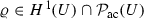
We study the McKean–Vlasov equation

$$\begin{aligned} \partial _t \varrho = \beta ^{-1} \Delta \varrho + \kappa {{\,\mathrm{\nabla \cdot }\,}}(\varrho \nabla (W \star \varrho )), \end{aligned}$$

with periodic boundary conditions on the torus. We first study the global asymptotic stability of the homogeneous steady state. We then focus our attention on the stationary system, and prove the existence of nontrivial solutions branching from the homogeneous steady state, through possibly infinitely many bifurcations, under appropriate assumptions on the interaction potential. We also provide sufficient conditions for the existence of continuous and discontinuous phase transitions. Finally, we showcase these results by applying them to several examples of interaction potentials such as the noisy Kuramoto model for synchronisation, the Keller–Segel model for bacterial chemotaxis, and the noisy Hegselmann–Krausse model for opinion dynamics.

1 Introduction

Systems of interacting particles arise in a myriad of applications ranging from opinion dynamics [41], granular materials [6, 11, 25] and mathematical biology [8, 47] to statistical mechanics [50], galactic dynamics [18], droplet growth [29], plasma physics [14], and synchronisation [48]. Apart from being of independent interest, these systems find applications in a diverse range of fields such as particle methods in numerical analysis [35], consensus-based methods for global optimisation [20], and nonlinear filtering [23]. They have also been studied in the context of multiscale analysis [40], in the presence of memory-like effects and in a non-Markovian setting [36], and in the discrete setting of graphs [38].

In this paper, we analyse the partial differential equation (PDE) associated to the system of interacting stochastic differential equations (SDEs) on ${{\mathbb {T}}}^d$, the torus of side length $L>0$, of the following form:

where the $X^i_t \in {{\mathbb {T}}}^d,i= 1\dots N$ represent the positions of the N “particles”, W is a periodic interaction potential, and the $B^i_t, i = 1 \dots N$ represent N independent ${{\mathbb {T}}}^d$-valued Brownian motions. The constants $\kappa ,\beta >0$ represent the strength of interaction and inverse temperature respectively. Since one of the two parameters is redundant, we keep $\beta$ fixed for the rest of the paper. It is clear that what we have described is a set of interacting overdamped Langevin equations. Based on the choice of W(x), one can then obtain models for numerous phenomena from the physical, biological, and social sciences. We refer to [45, 54, 55, 60] and the references therein for a comprehensive list of such models.

Systems of interacting diffusions have been studied extensively. They were first analysed by McKean (cf. [51, 52]) who noticed an interesting relation between them and a class of nonlinear parabolic partial differential equations. In particular, it is well known (cf. [58, 65]) that for this class of SDEs one can pass to the so-called mean field limit; if we consider the empirical measure defined as follows:

$$\begin{aligned} \varrho ^{(N)} : = \frac{1}{N} \sum \limits _{i=1}^N \delta _{X^i_t}, \quad \text { with }\quad {\text {Law}}(X_0:=(X^1_0 \cdots X^N_0 )) =\prod \limits _{i=1}^N \varrho _0({x_i}), \end{aligned}$$

then, provided that W is smooth, as $N \rightarrow \infty$, ${\mathbb {E}}(\varrho ^{(N)})$ converges in the sense of weak convergence of probability measures to some measure $\varrho$ satisfying the nonlocal parabolic PDE

$$\begin{aligned} \begin{aligned} \partial _t \varrho&= \beta ^{-1} \Delta \varrho + \kappa \nabla \cdot (\varrho \nabla W \star \varrho ), \\ \varrho (x,0)&=\varrho _0(x). \end{aligned} \end{aligned}$$

(1.1)

The above equation is commonly referred to as the McKean–Vlasov equation, the latter name stemming from the fact that it also arises as the overdamped limit of the Vlasov–Fokker–Planck equation. Equation (1.1) can also be thought of as a nonlinear Fokker–Planck equation for the following nonlinear SDE, commonly referred to as the McKean SDE:

where $\varrho = \text {Law}(X_t)$. The PDE (1.1) itself has a very rich structure associated to it - we have the following free energy functional:

(1.2)

where $S(\varrho )$ and ${\mathcal {E}}(\varrho ,\varrho )$ represent the entropy and interaction energy associated with $\varrho$ respectively. It is well known, starting from the seminal work in [43, 59], that this equation belongs to a larger class of dissipative PDEs including the heat equation, the porous medium equation, and the aggregation equation, which can be written in the form

$$\begin{aligned} \partial _t \varrho = \nabla \cdot \left( \varrho \nabla \frac{\delta {\mathscr {F}}}{\delta \varrho }\right) \, \end{aligned}$$

for some free energy ${\mathscr {F}}$, and are gradient flows for the associated free energy functional with respect to the $d_2$ transportation distance defined on probability measures having finite second moment, see [25, 69]. We refer the reader to [2, 63] for more information on the abstract theory of gradient flows in the space of probability measures.

Our goals are to study some aspects of the asymptotic behaviour and the stationary states of the McKean–Vlasov equation for a wide class of interaction potentials. In terms of the asymptotic behaviour, we analyse the stability conditions for the homogeneous steady state $1/L^d$ and the rate of convergence to equilibrium. We extend the ${L}^2$-decay results of [21] to arbitrary dimensions and arbitrary sufficiently nice interactions and also provide sufficient conditions for convergence to equilibrium in relative entropy.

The rest of the paper is devoted to the analysis of the properties of non-trivial stationary states of the Mckean–Vlasov system, that is, nontrivial solutions of

$$\begin{aligned} \beta ^{-1} \Delta \varrho + \kappa \nabla \cdot (\varrho \nabla W \star \varrho )=0. \end{aligned}$$

Previous results in this direction include those by Tamura [66], who provided some criteria for the existence of local bifurcations on the whole space by using tools from nonlinear functional analysis, in particular, the Crandall–Rabinowitz theorem. Unfortunately, his analysis depends crucially on the unphysical assumption that the interaction potential is an odd function. One of the main results of the present work is a complete, quantitative, local bifurcation analysis under physically realistic assumptions. Dawson [32] studied for the first time the existence of nontrivial stationary states for a particular double-well confinement and Curie–Weiss interaction on the line. The existence of nontrivial stationary states or the bifurcation of nontrivial solutions from the homogeneous steady state is usually referred as phase transition in the literature. We also mention that more recently several authors [9, 34, 68] looked at the existence of phase transitions in the whole space with different confinement and interactions. The most related work to us in the literature is due to Chayes and Panferov [27], who studied the problem on the torus and provided some criteria for the existence of continuous and discontinuous phase transitions.

In addition to presenting an existence and uniqueness theory for the evolution problem, we extend considerably the results of both [66] and [27]. We provide explicit criteria based on the Fourier coefficients of the interaction potential W for the existence of local bifurcations by studying the implicit symmetry in the problem. In fact, we show that for carefully chosen potentials it is possible to have infinitely many bifurcation points. Additionally, we extend the results of [27] and provide additional criteria for the existence of continuous and discontinuous phase transitions.

1.1 Statement of Main Results

We only state simplified versions of our results in one dimension, so as to avoid the use of notation that will be introduced later. We only need to define the cosine transform, for $k \in {{\mathbb {Z}}}, k>0$. We work with classical solutions of (1.1) which are constructed in Theorem 2.2.

Theorem 1.1

(Convergence to equilibrium) Let $\varrho$ be a classical solution of the Mckean–Vlasov equation (1.1) with smooth initial data and smooth, even, interaction potential W. Then we have:

• (a) If $0< \kappa < \frac{2 \pi }{3 \beta L ||\nabla W||_\infty }$, then $\left||\varrho (\cdot ,t)- \frac{1}{L}\right||_2 \rightarrow 0$, exponentially, as $t \rightarrow \infty$,

• (b) If ${\widetilde{W}}(k) \geqq 0$ for all $k \in {{\mathbb {Z}}}, k>0$, or $0< \kappa < \frac{2 \pi ^2}{ \beta L^2 ||\Delta W||_\infty }$, then ${\mathcal {H}}\left( \varrho (\cdot ,t)|\frac{1}{L}\right) \rightarrow 0$, exponentially, as $t \rightarrow \infty$

where denotes the relative entropy.

The previous theorem implies that the uniform state can fail to be the unique stationary solution only if the interaction potential has a negative Fourier mode, that is, the interaction potential is not H-stable. Thus, the concept of H-stability introduced by Ruelle [62] is relevant for the study of the stationary McKean–Vlasov equation as noticed in [27]. We have the following conditions for the existence of bifurcating branches of steady states:

Theorem 1.2

(Local bifurcations) Let W be smooth and even and let $(1/L,\kappa )$ represent the trivial branch of solutions. Then every $k^* \in {{\mathbb {Z}}}, k^*>0$ such that

• (1) ${\text {card}}\left\{ k \in {{\mathbb {Z}}}, k>0 : {\widetilde{W}}(k)={\widetilde{W}}(k^*)\right\} =1$,

• (2) ${\widetilde{W}}(k^*) <0$,

leads to a bifurcation point $(1/L,\kappa _*)$ of the stationary McKean–Vlasov equation through the formula

$$\begin{aligned} \kappa _*=-\frac{(2L)^{1/2}}{\beta {\widetilde{W}}(k^*)}. \end{aligned}$$

We are also able to sharpen sufficient conditions for the existence of continuous or discontinuous bifurcating branches. The following theorem is a simplified version of the exact statements that are presented in Theorem 5.11 and Theorem 5.19:

Theorem 1.3

(Discontinuous and continuous phase transitions) Let W be smooth and even and assume the free energy ${\mathscr {F}}_{\kappa ,\beta }$ defined in (1.2) exhibits a transition point, $\kappa _c<\infty$, in the sense of Definition 5.1. Then we have the following two scenarios:

• (a) If there exist strictly positive $k^a,k^b,k^c \in {{\mathbb {Z}}}$ with ${\widetilde{W}}(k^a)\approx {\widetilde{W}}(k^b)\approx {\widetilde{W}}(k^c)\approx \min _k{\widetilde{W}}(k)<0$ such that $k^a=k^b +k^c$, then $\kappa _c$ is a discontinuous transition point.

• (b) Let $k^\sharp = {{\,\mathrm{\mathrm{arg\,min}}\,}}_k {\widetilde{W}}(k)$ be uniquely defined with ${\widetilde{W}}(k^\sharp )<0$ and $\kappa _\sharp =\sqrt{2L}/(\beta {\widetilde{W}}(k^\sharp ))$. Let $W_\alpha$ denote the potential obtained by multiplying all the negative Fourier modes ${\widetilde{W}}(k)$ except ${\widetilde{W}}(k^\sharp )$ by some $\alpha \in (0,1]$. Then if $\alpha$ is made small enough, the transition point $\kappa _c$ is continuous and $\kappa _c=\kappa _\sharp$.

The proof of the above theorem relies mainly on Proposition 5.8 which states that if $\varrho _\infty$ is the unique minimiser of the free energy ${\mathscr {F}}_\kappa$ at $\kappa =\kappa _\sharp$ then $\kappa _c=\kappa _\sharp$ is a continuous transition point; on the other hand if $\varrho _\infty$ is not the global minimiser of ${\mathscr {F}}_\kappa$ at $\kappa =\kappa _\sharp$, then $\kappa _c<\kappa _\sharp$ and $\kappa _c$ is a discontinuous transition point.

We conclude the introduction with a figure to provide the reader with some more intuition about the spectral signature of continuous and discontinuous phase transitions. As it can be seen in Figure 1, the results of Theorem 1.3 essentially apply to two perturbative regimes. Figure 1(a) shows the scenario for the existence of a discontinuous transition point in which there are multiple resonating/near-resonating dominant modes $k^a,k^b,k^c$ which satisfy the algebraic condition $k^a=k^b+k^c$ from Theorem 1.3(a). This condition allows us to construct a competitor state at $\kappa =\kappa _\sharp$ which has a lower value of ${\mathscr {F}}_\kappa$ than $\varrho _\infty$ by controlling the sign of the higher order terms in the Taylor expansion of the free energy. The statement Theorem 1.3(a) is then a direct consequence of Proposition 5.8.

Figure 1(b) shows the scenario in which there is one dominant negative mode and all other negative modes are restricted to a small neighbourhood of 0. In this case, there exists a continuous transition point. The proof follows by showing that $\varrho _\infty$ is the unique minimiser of ${\mathscr {F}}_\kappa$ at $\kappa =\kappa _\sharp$. For controlling the involved error terms, the neighbourhood needs to made by small, which is equivalent to making $\alpha$ small in the statement of  Theorem 1.3(b). As it will become clear in §5, the condition in Theorem 1.3(b) is essentially an assumption on the size of the spectral gap of the linearised McKean–Vlasov operator. Again, applying Proposition 5.8, the result follows.

Fig. 1

a The near-resonating modes scenario, in which the modes $k^a=7,k^b=5,k^c=2$ satisfy the algebraic condition $k^a=k^b+k^c$; b The dominant mode scenario

This work provides a complete local and global bifurcation analysis for the Mckean–Vlasov equation on the torus. This enables us to study phase transitions for several important models that have been introduced in the literature. This is done in §6. In particular, we apply our results to the following examples: the noisy Kuramoto model for synchronisation, the Hegselmann–Krausse model for opinion dynamics, the Keller–Segel model for bacterial chemotaxis, the Onsager model for liquid crystal alignment, and the Barré–Degond–Zatorska model for interacting dynamical networks. As an example of the typical bifurcation diagram expected for this kind of system, we discuss the noisy Kuramoto model which has the interaction potential $W(x)=-(2/L)^{1/2}\cos (2 \pi x/L)$. For $\kappa$ sufficiently small, the uniform state is the unique stationary solution. At some critical $\kappa =\kappa _c$ a clustered solution branches out from the uniform state and for all $\kappa >\kappa _c$ this clustered state is preferred solution, that is, it is the global minimiser of the free energy, ${\mathscr {F}}_{\kappa }$. The bifurcation diagram and a plot of the clustered solution can be seen in Figure 2. The model is discussed in more detail in §6.1.

Fig. 2

a The bifurcation diagram for the noisy Kuramoto system: the solid blue line denotes the stable branch of solutions while the dotted red line denotes the unstable branch of solutions. b An example of a clustered solution representing phase synchronisation of the oscillators

1.2 Organisation of the Paper

The paper is organised in the following manner: in Section 2 we introduce the main notation and assumptions on the interaction potential W, state a basic existence and uniqueness theorem for classical solutions of the evolutionary problem and present a series of results about the stationary problem and the associated free energy that we use for our later analysis. In Section 3 we present the proof of Theorem 1.1(b), whereas the proof of  Theorem 1.1(a) is similar to the argument in [21] and can be found in Version 1 of the arXiv manuscript. Additionally, we perform a linear stability analysis of the Mckean–Vlasov PDE about $1/L^d$. Section 4 is dedicated mainly to the the proof of Theorem 1.2, including further details about the structure of the bifurcating branches and the structure of the global bifurcation diagram. In Section 5 we give sufficient conditions for the existence of continuous and discontinuous phase transitions and we present the proofs of Theorem 1.3(a) and Theorem 1.3(b), along with some supplementary results. In Section 6, we apply our results to various models from the biological, physical and social sciences.

2 Preliminaries

2.1 Set Up and Notation

Let $U={{{\mathbb {R}}}^{d}/ L {{\mathbb {Z}}}^d} \widehat{=} \left( -\frac{L}{2},\frac{L}{2}\right) ^d \subset {{\mathbb {R}}}^d$ be the torus of size $L>0$. We denote by ${{\mathbb {N}}}= \{0,1,\dots \}$ the nonnegative integers. Furthermore, we will denote by $\mathcal {P}(U)$ the space of Borel probability measures on U, by the subset of $\mathcal {P}(U)$ absolutely continuous with respect to the Lebesgue measure, and by the subset of having strictly positive densities almost everywhere. Additionally, $C^k(U)$ will denote the restriction to U of all L-periodic and k-times continuously differentiable functions, ${\mathcal {D}}(U)$ the space of test functions, and $\left\langle f,g\right\rangle _\mu$ the ${L}^2(U,\mu )$ inner product.

2.2 Assumptions on W

Throughout the subsequent discussion we will assume that W(x) is at least integrable and coordinate-wise even, that is

$$\begin{aligned}&\forall x\in {{\mathbb {R}}}^d \ \forall i \in \{1,\dots , d\} : \qquad W(x_1, \dots ,x_i, \dots , x_d)\\&\quad =W(x_1, \dots ,-x_i, \dots , x_d). \end{aligned}$$

For the evolutionary problem we will assume

while for the stationary problem we will assume

where the ${L}^p(U)$ with $1 \leqq p \leqq \infty$ represent the Lebesgue spaces and ${{\mathcal {W}}}^{k,p}(U)$ represent the periodic Sobolev spaces with ${H}^k(U) = {{\mathcal {W}}}^{k,2}(U)$. Wherever required, weaker or stronger assumptions will be indicated in the text. As one may expect, the assumptions on W(x) for the evolutionary and stationary problems to be the same, it is important to mention that these assumptions are in no way sharp and the aim of this paper is not to study low regularity theory for this class of PDEs.

For the space ${L}^2(U)$ we define the orthonormal basis, $\{w_k\}_{k \in {{\mathbb {Z}}}^d}$, $k=(k_1, k_2, \ldots , k_d)$, as follows:

$$\begin{aligned} w_k(x)= N_k\prod \limits _{i=1}^d w_{k_i}(x_i), \qquad \text { where } \qquad w_{k_i}(x_i)= {\left\{ \begin{array}{ll} \cos \left( \frac{2 \pi k_i}{L} x_i\right) &{} k_i>0, \\ 1 &{} k_i=0, \\ \sin \left( \frac{2 \pi k_i}{L} x_i\right) &{} k_i<0, \\ \end{array}\right. } \end{aligned}$$

(2.1)

and $N_k$ is defined as

$$\begin{aligned} N_k:=\frac{1}{L^{d/2}}\prod \limits _{i=1}^d \left( 2-\delta _{k_i, 0} \right) ^{\frac{1}{2}}=: \frac{\Theta (k)}{L^{d/2}}, \end{aligned}$$

(2.2)

where $\delta _{i,j}$ denotes the Kronecker delta. We then have the following form for the discrete Fourier transform of any $f \in {L}^2(U)$:

$$\begin{aligned} {\widetilde{f}}(k)&= \langle f,w_k \rangle , \qquad k \in {{\mathbb {Z}}}^d. \end{aligned}$$

We denote by “$\star$” the convolution of any two functions, $f(x),g \in {L}^2(U)$ and for $f(x)=W(x)$ we have the following representation in Fourier space:

$$\begin{aligned} (W \star g)(y)= \sum \limits _{k \in {{\mathbb {N}}}^d}{\widetilde{W}}(k) \frac{1}{N_k} \sum \limits _{\sigma \in \mathrm {Sym}(\Lambda )}{\widetilde{g}}(\sigma (k))w_{\sigma (k)}(y). \end{aligned}$$

Here, we have used the fact that W(x) is coordinate-wise even. $\mathrm {Sym}(\Lambda )$ represents the symmetry group of the product of two-point spaces $\Lambda =\{1,-1\}^d$, which acts on ${{\mathbb {Z}}}^d$ by pointwise multiplication, that is, $(\sigma (k))_i=\sigma _i k_i, k \in {{\mathbb {Z}}}^d, \sigma \in \mathrm {Sym}(\Lambda )$. Another expression that we will use extensively in the sequel is the Fourier expansion of the following bilinear form:

(2.3)

It will be useful to note that for any function g(x) and $k \in {{\mathbb {Z}}}^d$ the sum $\sum _{\sigma \in \mathrm {Sym}(\Lambda )}|{\widetilde{g}}(\sigma (k))|^2$ is translation invariant, that is, the value of the sum is the same for g and $g_\tau (x) =g(x+\tau )$ for $\tau \in U$. In later sections we will also use the space ${L}^2_s(U) \subset {L}^2(U)$, which we define as the space of coordinate-wise even functions in ${L}^2(U)$ given by

$$\begin{aligned} {L}^2_s(U)= & {} \{ f\in {L}^2(U) : f(x_1,\dots ,x_i,\dots ,x_d)\nonumber \\= & {} f(x_1,\dots ,-x_i,\dots , x_d), i\in \{1,\dots ,d\} , x\in U \}. \end{aligned}$$

(2.4)

It should be noted that any pointwise properties (like being coordinate-wise even) should be understood in a pointwise almost everywhere sense. The space ${L}^2_s(U)$ is a closed subspace of ${L}^2(U)$ and thus is a Hilbert space in its own right. It is also easy to check that $\{w_k\}_{k \in {{\mathbb {N}}}^d} \subset \{w_k\}_{k \in {{\mathbb {Z}}}^d}$ forms an orthonormal basis for ${L}^2_s(U)$. If g is assumed to be in ${L}^2_s(U)$, then the above expressions reduce to

In addition, the sign of the individual Fourier modes of W is quite important in the subsequent analysis and we introduce the following definition:

Definition 2.1

A function $W \in {L}^2(U)$ is said to be H-stable, denoted by $W \in {{\mathbb {H}}}_\text {s}$, if it has non-negative Fourier coefficients, i.e,

$$\begin{aligned} {\widetilde{W}}(k) \geqq 0, \quad \forall k \in {\mathbb {Z}}^d, \end{aligned}$$

where, ${\widetilde{W}}_k=\langle W,w_k\rangle$. This is, by (2.3), equivalent to the condition that

Thus every potential is decomposed into two parts $W(x)=W_\text {s}(x) + W_\text {u}(x)$, where

$$\begin{aligned} W_\text {s}(x)&= \sum \limits _{k \in {{\mathbb {Z}}}^d} \left( \langle W,w_k\rangle \right) _+ w_k(x)\qquad \text {and}\qquad W_\text {u}(x)=W(x)-W_\text {s}(x). \end{aligned}$$

Hereby, $(a)_+ = \max \{0, a\}$ (resp. $(a)_-= \min \{0, a\}$) denotes the positive (resp. negative) part for a real number $a\in {{\mathbb {R}}}$. We will denote a potential $W \in {L}^2(U)$ which is not H-stable by $W \in {{\mathbb {H}}}_s^c$.

An immediate consequence of the identity (2.3) is that H-stable potentials have nonnegative interaction energy. The above definition can be thought of as a continuous analogue of the notion of H-stability encountered in the study of discrete systems (cf. [62]). We refer to [26] for an example of the notion of H-stability applied to continuous systems. For the rest of the paper we will drop the subscript U under the integral sign and all integrals in space will be taken over U unless specified otherwise.

2.3 Existence and Uniqueness for the Dynamics

We present an existence and uniqueness result for the McKean–Vlasov equation and comment on the nontrivial parts of the proof. The proof is quite standard. Our result is an extension of [21, Theorem 4.5] since we consider all potentials W satisfying Assumption (A1) in any dimension d, as opposed to [21, Theorem 4.5] which deals with the Hegselmann–Krause potential in one dimension. Additionally, we prove strict positivity of solutions as opposed to the nonnegativity proved in [21]. We prove below the existence of classical solutions $\varrho (\cdot ,t) \in C^2 (U)$ to the system

$$\begin{aligned} \begin{aligned} \frac{\partial \varrho }{\partial t}&= \beta ^{-1}\Delta \varrho + \kappa {{\,\mathrm{\nabla \cdot }\,}}(\varrho \nabla W \star \varrho ), \qquad&(x,t) \in U \times (0,T] \ ; \\ \varrho (x,0)&=\varrho _0(x), \qquad&x \in U. \end{aligned} \end{aligned}$$

(2.5)

Theorem 2.2

Assume Assumption (A1) holds, then for , there exists a unique classical solution $\varrho$ of (2.5) such that for all $t>0$. Additionally, $\varrho (\cdot ,t)$ is strictly positive and has finite entropy, i.e, $\varrho (\cdot ,t)>0$ and $S(\varrho (\cdot ,t))< \infty$, for all $t>0$.

The strategy of the proof is identical to that used in the proof of [21, Theorem 4.5]. We construct a sequence of linear problems that approximate the McKean–Vlasov equation

$$\begin{aligned} \frac{\partial \varrho _n}{\partial t} = \beta ^{-1}\Delta \varrho _n + \kappa {{\,\mathrm{\nabla \cdot }\,}}(\varrho _n\nabla W \star \varrho _{n-1}) \quad&\text { in } U \times (0,T], \\ \forall i \in \{1,\dots , d\} : \qquad \varrho _n(\cdot + L {\mathbf {e}}_i)=\varrho _n(\cdot ) \quad&\text { on } \partial U \times [0,T], \\ \varrho =\varrho ' \quad&\text { in } U \times \{0\}, \end{aligned}$$

which for smooth initial data, have unique smooth solutions. Similar apriori estimates to [21] obtained using the ${{\mathcal {W}}}^{2,\infty }(U)$-regularity of W allows us to pass to the limit as $n \rightarrow \infty$ and recover weak solutions of the McKean–Vlasov equation which are proved to be unique. Their regularity follows from bootstrapping and using the regularity of W and the initial data.

We now comment on the proof of strict positivity for classical solutions $\varrho (x,t)$ of (2.5). The nonnegativity of the solutions follows from a similar argument to [21, Corollary 2.2]. Consider now the “frozen” linearised version of the McKean–Vlasov equation, that is,

$$\begin{aligned} \frac{\partial \vartheta }{\partial t}= {{\,\mathrm{\nabla \cdot }\,}}\left( \beta ^{-1}\nabla \vartheta + \kappa \vartheta (\nabla W \star \varrho (x,t))\right) . \end{aligned}$$

This is a linear parabolic PDE with uniformly bounded and continuous coefficients. Additionally, $\varrho (x,t)$ is a classical solution to this PDE. Thus we have a Harnack’s inequality of the following form (cf. [16, Theorems 8.1.1-8.1.3] for sharp versions of this result):

$$\begin{aligned} \sup _U \varrho (x,t_1) < C \inf _U \varrho (x,t_2), \end{aligned}$$

for $0<t_1<t_2< \infty$ for some positive constant C. Since $\varrho (x,t)$ is nonnegative and $||\varrho (x,t)||_{1}=1$ for all $0\leqq t < \infty$, this implies that $\inf _U\varrho (x,t)$ is positive for any positive time. The fact that the entropy is finite follows from the fact that $\varrho (x,t)$ is positive and bounded above.

2.4 Characterisation of the Stationary Solutions

In subsequent sections we will study the stationary solutions of the McKean–Vlasov equation (2.5), i.e, classical solutions $\varrho \in C^2 (U)$ of

$$\begin{aligned} {{\,\mathrm{\nabla \cdot }\,}}\left( \beta ^{-1}\nabla \varrho + \kappa \varrho \nabla W \star \varrho \right) =0, \quad&x \in U . \end{aligned}$$

(2.6)

In this subsection we present standard results about the stationary McKean–Vlasov equation that will be useful for our later analysis. The main results in this section are Theorem 2.3 which discusses the existence of solutions and their regularity, Proposition 2.4 which connects stationary solutions to minimisers of the free energy, and Theorem 2.7 which discusses the existence of minimisers for the free energy.

We start by discussing the existence and and regularity question for the stationary problem. The proof relies on the link between the stationary PDE and the fixed points of a nonlinear map as was discussed in [66] and [37].

Theorem 2.3

(Existence, regularity, and strict positivity of solutions for the stationary problem) Consider the stationary McKean–Vlasov PDE (2.6) such that Assumption (A2) holds. Then we have that

• (a) There exists a weak solution, of (2.6) and any weak solution is a fixed point of the nonlinear map

  

  (2.7)

• (b) Any weak solution is smooth and strictly positive, that is, .

Proof

The weak formulation of (2.6) is

(2.8)

where we look for solutions . We have the following estimate on the map ${\mathcal {T}}$ from (2.7):

$$\begin{aligned} \left||{\mathcal {T}}\!\varrho \right||_2^2 \leqq \left||{\mathcal {T}}\!\varrho \right||_\infty \leqq e^{\beta \kappa (\left||W_-\right||_\infty + \left||W\right||_1)}. \end{aligned}$$

(2.9)

Thus it makes sense to search for fixed points of this equation in the set as all fixed points must be in this set. It is easy to check that E is a closed, convex subset of ${L}^2(U)$. We can now redefine ${\mathcal {T}}$ to act on E. Additionally, for any $\varrho \in E$, we have that

$$\begin{aligned} \left||{\mathcal {T}}\!\varrho \right||_{{H}^1}^2&= \left||{\mathcal {T}}\!\varrho \right||_2^2 + \left||\nabla {\mathcal {T}}\!\varrho \right||_2^2 \leqq \left||{\mathcal {T}}\!\varrho \right||_\infty \left( 1 + L^d\beta ^2 \kappa ^2 \left||{\mathcal {T}}\!\varrho \right||_\infty ^2\left||\nabla W\right||_2^2\right) \ , \end{aligned}$$

(2.10)

where we have used the fact that $W \in {H}^1(U)$. Thus, using (2.9), we have that ${\mathcal {T}}(E) \subset E$ is uniformly bounded in ${H}^1(U)$. By Rellich’s compactness theorem, this implies that ${\mathcal {T}}(E)$ is relatively compact in ${L}^2(U)$, and therefore in E, since E is closed. Furthermore, ${\mathcal {T}}$ is Lipschitz continuous, that is, we have for $\varrho _1,\varrho _2 \in E:$$\left||{\mathcal {T}}\!\varrho _1 -{\mathcal {T}}\!\varrho _2\right||_2 \leqq C\left||\varrho _1-\varrho _2\right||_2$, for some positive constant C. By the Schauder fixed point theorem, there exists a fixed point of $\varrho \in E$ of ${\mathcal {T}}$ which by (2.10) is in ${H}^1(U)$. Plugging this expression into the weak form of the PDE (2.8) we obtain (a). Also note that fixed points of ${\mathcal {T}}$ are bounded from below by $e^{-\beta \kappa (\left||W_-\right||_\infty + \left||W\right||_1 \left||{\mathcal {T}}\!\varrho \right||_\infty )}$, proving the positivity of them.

Before proceeding to the proof of (b), we argue that every weak solution in is a fixed point of the nonlinear map, ${\mathcal {T}}$. Considering the “frozen” version of the weak form in (2.8),

(2.11)

where is a weak solution of (2.6) and $\vartheta$ is the unknown function. The above equation is the weak form of a uniformly elliptic PDE whose associated bilinear form is coercive in the weighted space, ${H}^1_0(U, {\mathcal {T}}\!\varrho )$ where ${H}^1_0(U)={H}^1(U) /\ {{\mathbb {R}}}$. To see this, set $\vartheta (x)=h(x) {\mathcal {T}}\!\varrho$. We then obtain the following integral formulation of the transformed PDE:

Let $h_1$ and $h_2$ be two weak solutions of the above equation. By choosing $\varphi =h_1 -h_2 = h$, we obtain a unique weak solution to (2.11) up to normalisation. Here, we also used that ${\mathcal {T}}\!\varrho$ has full support, since it is bounded from below. Hence, if it is chosen to be a probability measure, it is unique. We observe that $\vartheta ={\mathcal {T}}\!\varrho$ is such a weak solution, as is $\varrho$. This implies that any weak solution must be such that $\varrho ={\mathcal {T}}\!\varrho$.

We obtain regularity of solutions by observing that if $f \in {H}^m(U), g \in {H}^n(U)$, then we have that $f \star g \in {{\mathcal {W}}}^{m+n,\infty }(U)$. Then we use a bootstrap argument, that is, $W \in {H}^1(U), \varrho \in {H}^1(U)$ implies that $\varrho ={\mathcal {T}}\!\varrho \in {{\mathcal {W}}}^{2,\infty }(U)$. This implies that $W \star \varrho \in {{\mathcal {W}}}^{3,\infty }(U)$ and so on and and so forth. Thus we have that $\varrho \in {H}^m(U) \cup {{\mathcal {W}}}^{m,\infty }(U)$ for any $m \in {{\mathbb {N}}}$. The strict positivity follows from the lower bound on ${\mathcal {T}}\!\varrho$. $\quad \square$

We already know that associated with this PDE we have a free energy functional defined on the space of strictly positive absolutely continuous probability measures on U by

(2.12)

Since we regard $\beta$ as a fixed parameter, we omit it in the subscript on ${\mathcal {F}}_\kappa$.

The free energy ${\mathscr {F}}_{\kappa }$ is a Lyapunov function for the evolution and its negative derivative along the flow is given by the entropy dissipation functional with

This follows from rewriting (2.5) as $\partial _t \varrho = {{\,\mathrm{\nabla \cdot }\,}}\left( \varrho \left( \beta ^{-1} \nabla \log \varrho + \nabla W \star \varrho \right) \right)$ and differentiating the free energy functional along the flow

Finally we have the Gibbs state map . This equation encodes the stationary states as fixed points of the nonlinear mapping ${\mathcal {T}}$ from (2.7):

(2.13)

The identification of stationary states (2.6), critical points of ${\mathscr {F}}_{\kappa }$ and $\mathcal {J}_\kappa$, and zeros of $F_{\kappa }$ is given by the following proposition:

Proposition 2.4

Assume W(x) satisfies Assumption (A2) and fix $\kappa >0$. Let . Then the following statements are equivalent:

• (1) $\varrho$ is a classical solution of the stationary McKean–Vlasov equation (2.6).

• (2) $\varrho$ is a zero of the map $F_\kappa (\varrho )$.

• (3) $\varrho$ is a critical point of the free energy ${\mathscr {F}}_\kappa (\varrho )$.

• (4) $\varrho$ is a global minimiser of the entropy dissipation functional ${\mathcal {J}}_\kappa (\varrho )$.

Proof

• (1)$\Leftrightarrow$(2): Observe that $\varrho$ is a zero of $F_\kappa (\varrho )$ if and only if it is a fixed point of ${\mathcal {T}}$. Thus by part (a) of Theorem 2.3 we have the desired equivalence.

• (2)$\Rightarrow$(3): The main observation for this is that zeroes of $F_\kappa$ represent solutions of the Euler–Lagrange equations for ${\mathscr {F}}_\kappa$. Let , we define the standard convex interpolant, $\varrho _s=(1-s)\varrho +s \varrho _1$, $s \in (0,1)$ such that ${\mathscr {F}}(\varrho ),{\mathscr {F}}(\varrho _1)< \infty$. Then we have the following form of the Euler–Lagrange equations (which are well-defined for ):

  

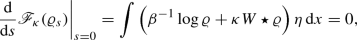  (2.14)

  where $\eta = \varrho _1-\varrho$. Now if $\varrho$ is a zero of $F_\kappa$ it is easy to check that the above expression is zero for any .

• (3)$\Rightarrow$(2): On the other hand assume that $\varrho$ is a critical point. If the integrand $\beta ^{-1}\log \varrho + \kappa W \star \varrho$ in (2.14) is not constant almost everywhere, we can find without loss of generality a set $A \in \mathcal {B}(U)$ of nonzero Lebesgue measure such that

  

  We are now free to choose to be

  $$\begin{aligned} \varrho _1 = \frac{1}{L^d}\left( {(1- \varepsilon ) \chi _A(x) + \varepsilon \chi _A^c(x)}\right) \ \end{aligned}$$

  for some $\varepsilon >0$. For this choice of $\varrho _1$, we have,

  

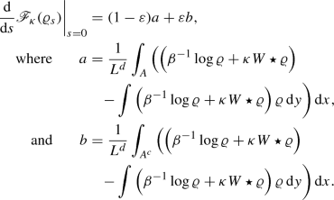
  From our choice of the set A, it is clear that $a >0$ and $b \leqq 0$. Since $\varepsilon$ can be made arbitrarily small, $(1-\varepsilon )a + \varepsilon b$ can be made positive. Thus we have derived a contradiction, since $\varrho$ is a critical point of ${\mathscr {F}}_\kappa$ and therefore it must satisfy the Euler–Lagrange equations in (2.14). Thus the integrand must be constant almost everywhere from which we obtain (3)$\Rightarrow$(2).

• (2)$\Rightarrow$(4): Clearly, ${\mathcal {J}}_\kappa$ is nonnegative. Thus if ${\mathcal {J}}_\kappa (\varrho )=0$ for some then it is necessarily a global minimiser. Plugging in $\varrho$ for some zero of $F_\kappa$ finishes this implication.

• (4)$\Rightarrow$(2): Now, any global minimiser $\varrho$ of ${\mathcal {J}}_\kappa (\varrho )$ must satisfy ${\mathcal {J}}_\kappa (\varrho )=0$ since ${\mathcal {J}}_\kappa (\varrho _\infty )=0$. From the expression for ${\mathcal {J}}_\kappa (\varrho )$ and the fact that $\varrho$ has full support this is possible only if

  $$\begin{aligned} \nabla \frac{ \log \varrho }{e^{-\beta \kappa W \star \varrho }} =0, \quad {\mathrm {almost everywhere}}. \end{aligned}$$

  Thus, we have that, $\varrho - C e^{-\beta \kappa W \star \varrho }=0$, almost everywhere, for some constant, $C>0$, which is given precisely by $Z(\varrho ,\kappa ,\beta )$ since . Thus we have that $\varrho$ is a zero of $F_\kappa (\varrho )$ and the reverse implication, (4)$\Rightarrow$(2).

 $\quad \square$

The following lemma is taken from [27] in which it is shown that for any unbounded there exists a bounded having a lower value of the free energy:

Lemma 2.5

([27]) Assume that W satisfies Assumption (A2) and fix $\kappa \in (0, \infty )$. Then there exists a positive constant $B_0<\infty$ such that for all with $\left||\varrho \right||_{\infty } > B_0$ there exists some with $\left||\varrho ^{\dagger }\right||_{\infty }\leqq B_0$ satisfying

$$\begin{aligned} {\mathscr {F}}_{\kappa }(\varrho ^{\dagger }) < {\mathscr {F}}_{\kappa }(\varrho ). \end{aligned}$$

The next lemma shows that minimisers of ${\mathscr {F}}_\kappa (\varrho )$ over are attained in .

Lemma 2.6

Assume W(x) satisfies Assumption (A2) and let . Then, there exists such that

$$\begin{aligned} {\mathscr {F}}_\kappa (\varrho ^+) < {\mathscr {F}}_\kappa (\varrho ). \end{aligned}$$

Proof

Let ${{\mathbb {B}}}_0:=\{ x \in U:\varrho (x)=0\}$. Then, from assumption , it follows that $|{{\mathbb {B}}}_0|>0$. We define the competitor state

and show that for $\epsilon >0$ sufficiently small $\varrho _\epsilon$ has smaller free energy; we first compute its entropy

where we have used the fact that . For computing the interaction term, we use the fact that ${\mathcal {E}}(\varrho ,\varrho )> - \left||W_-\right||_\infty$ to estimate

where $C_1,C_2<\infty$ depend on W and ${{\mathbb {B}}}_0$ and we have chosen $\epsilon$ sufficiently small. Combining the two expressions together, we obtain

$$\begin{aligned} {\mathscr {F}}_\kappa (\varrho _\epsilon ) < {\mathscr {F}}_\kappa (\varrho ) +\frac{\epsilon |{{\mathbb {B}}}_0| }{1 + \epsilon |{{\mathbb {B}}}_0|}\left( \beta ^{-1} \log \epsilon -\beta ^{-1} S(\varrho _\infty ) + (C_1+C_2) \epsilon \right) . \end{aligned}$$

Thus for $\epsilon$ sufficiently small but positive the logarithmic term will dominate and give us the required result.  $\quad \square$

Theorem 2.7

(Existence of a minimiser [27]) Assume W(x) satisfies Assumption (A2). For $\kappa \in (0,\infty )$ the free energy ${\mathscr {F}}_{\kappa }(\varrho )$ has a smooth minimiser .

Proof

We start by noticing that we can control the entropy and interaction energy from below as follows:

$$\begin{aligned} S(\varrho ) \geqq \log \varrho _\infty \qquad \text {and}\qquad \mathcal {E}(\varrho ,\varrho ) \geqq -\left||W_-\right||_\infty , \end{aligned}$$

(2.15)

where the bound on the entropy follows from Jensen’s inequality and the bound on the interaction energy follows from Assumption (A2). Since by (2.15), ${\mathscr {F}}_{\kappa }(\varrho )$ is bounded from below over , there exists a minimising sequence . Furthermore, by Lemma 2.5, the minimising sequence can be chosen such that $\{\varrho _j\}_{j=1}^\infty \subset {L}^2(U)$ with $\left||\varrho _j\right||_2 \leqq B_0^{\frac{1}{2}}$, where $B_0$ is the constant from Lemma 2.5. Thus, there exists a subsequence which we continue to denote by $\{\varrho _j\}_{j=1}^\infty$ such that $\varrho _j \rightharpoonup \varrho _{\kappa }$ weakly in ${L}^2(U)$. Clearly we have that . It is also easy to see that $\varrho _\kappa \geqq 0$, almost everywhere. Thus . The lower semicontinuity of $S(\varrho )$ follows from standard results (cf. [44], Lemma 4.3.1). Consider now the interaction energy term. For $W \in {L}^1(U)$, the interaction energy is weakly continuous in ${L}^2(U)$ [27, Theorem 2.2, Equation (9)]. This implies that the free energy ${\mathscr {F}}_\kappa (\varrho )$ has a minimiser $\varrho _\kappa$ over . A direct consequence of this and Lemma 2.6 is that the minimisation problem is well-posed in since the minimiser $\varrho _\kappa$ must be attained in . We can then use Theorem 2.3 together with Proposition 2.4 to argue that any such minimiser must be smooth.  $\quad \square$

Proposition 2.8

Assume W satisfies Assumption (A2) such that $W_\text {u}$ is bounded from below, where $W_\text {u}$ is the unstable part defined in Definition 2.1. Then, for $\kappa \in \left( 0,\kappa _{\mathrm {con}}\right)$, where $\kappa _{\mathrm {con}}:=\beta ^{-1} \left||W_{\text {u}-}\right||_\infty ^{-1}$, the functional ${\mathscr {F}}_\kappa (\varrho )$ is strictly convex on , that is, for all $s\in (0,1)$, it holds that

Proof

For , let $\varrho (s)=(1-s) \varrho _1 + s \varrho _2, s \in (0,1)$ and $\eta =\varrho _2-\varrho _1$. Then we have

Now we apply Jensen’s inequality and use the fact that $W_\text {s}\in {{\mathbb {H}}}_\text {s}$, which gives us

Finally we bound $W_\text {u}(x)$ from below to obtain

showing the desired statement.  $\quad \square$

Remark 2.9

It follows from the above result that if $W_\text {u}\equiv 0$, that is, $W\in {{\mathbb {H}}}_\text {s}$, then ${\mathscr {F}}_\kappa (\varrho )$ is strictly convex for all $\kappa \in (0,\infty )$.

3 Global Asymptotic Stability

3.1 Trend to Equilibrium in Relative Entropy

In this section, we will use the free energy as defined in (2.12) to study the global asymptotic stability of the uniform state for the system (2.5). By introducing the relative entropy

(3.1)

we observe the following identity between the free energy gap and the relative entropy:

$$\begin{aligned} {\mathscr {F}}_\kappa (\varrho )-{\mathscr {F}}_\kappa (\varrho _{\infty }) = \beta ^{-1}\mathcal {H}(\varrho | \varrho _\infty ) + \frac{\kappa }{2}\mathcal {E}(\varrho -\varrho _\infty ,\varrho -\varrho _\infty ). \end{aligned}$$

By directly differentiating the relative entropy (3.1), we obtain the rate of change of the relative entropy:

(3.2)

Proposition 3.1

(Exponential stability and convergence in relative entropy) Let with $S(\varrho _0) <\infty$ and $W \in {{\mathcal {W}}}^{2,\infty }(U)$. Then the classical solution $\varrho$ of (2.5) is exponentially stable in relative entropy and it holds that

$$\begin{aligned} {\mathcal {H}}(\varrho (\cdot ,t) | \varrho _\infty ) \leqq \exp \left[ \left( -\frac{4 \pi ^2}{\beta L^2} +2 \kappa \left||\Delta W_\text {u}\right||_{\infty }\right) t \right] \ {\mathcal {H}}(\varrho _0 | \varrho _\infty ). \end{aligned}$$

Especially, in the cases $W \in {{\mathbb {H}}}_\text {s}$ for any $\beta ,\kappa >0$ and if $W\notin {{\mathbb {H}}}_\text {s}$ for $\beta \kappa < \frac{2\pi ^2}{L^2 \left||\Delta W_\text {u}\right||_{\infty }}$ it holds that we have exponentially fast convergence to the uniform state in relative entropy for any initial condition .

Proof of Theorem 1.1(b)

We know the solution $\varrho$ is classical, thus $\mathcal {H}(\varrho (\cdot ,t) | \varrho _\infty ) \in C^1(0,\infty )$. Using (3.2), we obtain, with another integration by parts,

The first term is the Fisher information and can be controlled by a log-Sobolev inequality of the form

(3.3)

Now, we rewrite the interaction term in its Fourier series by (2.3), estimate it in terms of the unstable modes and transform it back to position space

Now, we use the fact that $\Delta W_\text {u}$ has mean zero to replace $\varrho$ by $\varrho - \varrho _\infty$ and estimate

The above term can be controlled using the CKP inequality in the following way:

$$\begin{aligned} \left||\varrho - \varrho _\infty \right||_{1} \leqq \sqrt{2 \mathcal {H}(\varrho |\varrho _\infty )} . \end{aligned}$$

(3.4)

In combination with (3.3) and (3.4), we obtain the bound

Finally, by Gronwall’s inequality, we have the desired result.  $\quad \square$

Remark 3.2

For the case of the noisy Hegselmann–Krausse model studied in [21], we have with $\phi (|x|)={\mathbb {1}}_{|x|\leqq R}$. We can estimate by the same arguments $\left||W_\text {u}''(x)\right||_{\infty }\leqq \left||W''(x)\right||_{\infty }={R}$. Thus for $\kappa <\frac{2 \pi ^2}{\beta L^2}$, we have exponential convergence to equilibrium. See §6.2 for a detailed analysis of this model.

Remark 3.3

By the improved entropy defect estimate of Lemma 5.16, the above statement could be slightly improved under more specific assumptions on the unstable modes of the potential. For the moment, we want to keep the presentation as concise as possible and refer to §5 for the details.

3.2 Linear Stability Analysis

We start this subsection by linearising the stationary Mckean–Vlasov equation around some stationary solution, $\varrho _\kappa$. We obtain the following linear integrodifferential operator:

$$\begin{aligned} {\mathcal {L}}w := \beta ^{-1} \Delta w+ \kappa {{\,\mathrm{\nabla \cdot }\,}}\left( \varrho _\kappa \nabla (W \star w)\right) + \kappa {{\,\mathrm{\nabla \cdot }\,}}\left( w \nabla (W \star \varrho _\kappa )\right) . \end{aligned}$$

If we pick $\varrho _\kappa$ to be the uniform state $\varrho _\infty$, the above expression reduces to

$$\begin{aligned} {\mathcal {L}}w := \beta ^{-1} \Delta w+ \kappa \varrho _\infty \Delta (W \star w). \end{aligned}$$

We are now interested in studying the spectrum of this operator over mean zero ${L}^2(U)$ functions, ${L}^2_0(U)$. From the classical theory for symmetric elliptic operators, it follows that the eigenfunctions of this system form an orthonormal basis in ${L}^2_0(U)$ given by $\{ L^{-\frac{d}{2}} e^{i \frac{2 \pi }{L} k' \cdot x}\}_{k' \in {{\mathbb {Z}}}^d\setminus \{{\mathbf {0}}\}}$ with the eigenvalues given by

$$\begin{aligned} \lambda _{k'}= \left( -\beta ^{-1}\left( \frac{2 \pi |k'|}{L}\right) ^2 - \kappa L^{-d/2} \left( \frac{2 \pi |k'|}{L}\right) ^2 {\widehat{W}}(k') \right) , \end{aligned}$$

where . One can check that we have the following relationship:

$$\begin{aligned} {\widehat{W}}(k') = \frac{1}{\Theta (k)} {\widetilde{W}}(k), \qquad k_\ell = |k'_\ell |, \ k \in {{\mathbb {N}}}^d, \end{aligned}$$

where $\Theta (k)$ is as defined in (2.2). To obtain the above expression we have used the fact that W is coordinate-wise even, which implies that

Thus, we have the following expression for the value of the parameter $\kappa _\sharp$ at which the first eigenvalue of ${\mathcal {L}}$ crosses the imaginary axis:

$$\begin{aligned} \kappa _\sharp = -\frac{L^{d/2}\Theta (k)}{\beta \min _{k \in {{\mathbb {N}}}^d\setminus \{{\mathbf {0}}\}} {\widetilde{W}}(k)} \, . \end{aligned}$$

(3.5)

We will refer to $\kappa _\sharp$ as the point of critical stability. We denote by $k^\sharp$ the critical wave number (if it is unique) and define it as

$$\begin{aligned} k^\sharp := {{\,\mathrm{\mathrm{arg\,min}}\,}}_{k \in {{\mathbb {N}}}^d\setminus \{{\mathbf {0}}\}} {\widetilde{W}}(k) \, . \end{aligned}$$

(3.6)

4 Bifurcation Theory

For the local bifurcation analysis, it is convenient to rewrite the fixed point equation (2.13) of the nonlinear mapping (2.7) by making the parameter $\kappa \in (0,\infty )$ explicit. Hence, in this section we consider the nonlinear map $F:{L}^2_s(U) \times {{\mathbb {R}}}^+ \rightarrow {L}^2_s(U)$ defined as

(4.1)

where $\beta > 0$ is fixed, and $W \in {L}^2_s(U)$ with ${L}^2_s(U)$, the space of coordinate-wise even and square integrable functions as defined in (2.4).

The purpose of this section is to study the bifurcation problem

$$\begin{aligned} F(\varrho ,\kappa )=0. \end{aligned}$$

Any zero of $F(\varrho ,\kappa )$ is also a coordinate-wise even fixed point of . The converse is true if W satisfies Assumption (A2). We do not make this assumption for the whole section as we want the bifurcation theory to be valid for more singular potentials, for example, the Keller–Segel model which we treat in a later section. It is also clear that the map $F(\varrho ,\kappa )$ is translation invariant on the whole space ${L}^2_s(U)$, that is, if $\varrho$ is a zero of $F(\varrho ,\kappa )$ then so is any translate $\varrho (\cdot - y)$ of $\varrho (\cdot )$ for any $y\in U$. This is the motivation for the restriction of F to the space ${L}^2_s(U)$. We will further justify our choice of the space ${L}^2_s(U)$ in Lemma 5.18.

The first result is an easy consequence of the characterisation of stationary solutions from §2.4, but could be also derived by standard contraction mapping argument on the map F as done in [66, Theorem 4.1] and [53, Theorem 3].

Proposition 4.1

Assume W(x) satisfies Assumption (A2). Then, for $\kappa$ sufficiently small, the uniform state $\varrho _\infty$ is the only solution of $F(\varrho ,\kappa )=0$.

Proof

Proposition 2.8 implies that ${\mathscr {F}}_\kappa (\varrho )$ is strictly convex for $\kappa < \kappa _{\mathrm {con}} = \beta ^{-1} \left||W_\text {u}\right||_\infty ^{-1}$. Hence, using Theorem 2.7, it has a unique minimiser and exactly one critical point. This implies from Proposition 2.4 that $F(\varrho ,\kappa )$ has a unique solution.  $\quad \square$

We use the trivial branch of solutions $F(\varrho _\infty ,\kappa )=0, \kappa \in (0,\infty )$ with $\varrho _\infty \equiv 1/L^d$ to centre the map and define for any $u\in {L}^2_s(U)$

$$\begin{aligned} {\widehat{F}}(u,\kappa )=F(u + \varrho _\infty ,\kappa ). \end{aligned}$$

(4.2)

In this way, we have ${\widehat{F}}(0,\kappa )=0$. We compute the Fréchet derivatives of this map for variations $w_1,w_2, w_3\in {L}_s^2(U)$:

(4.3)

(4.4)

(4.5)

(4.6)

(4.7)

We have the following characterisation of the local bifurcations of ${\widehat{F}}$:

Theorem 4.2

Consider ${\widehat{F}}: {L}^2_s(U) \times {{\mathbb {R}}}^+ \rightarrow {L}^2_s(U)$ as defined in (4.1) with $W \in {L}^2_s(U)$. Assume there exists $k^* \in {{\mathbb {N}}}^d$ such that

• (1) ${\text {card}}\left\{ k : \frac{{\widetilde{W}}(k)}{\Theta (k)}=\frac{{\widetilde{W}}(k^*)}{\Theta (k^*)}\right\} =1$;

• (2) ${\widetilde{W}}(k^*) <0$.

Then $(0,\kappa _*)\in {L}^2_s(U) \times {{\mathbb {R}}}^+$ is a bifurcation point of ${\widehat{F}}(\varrho ,\kappa )=0$ where

$$\begin{aligned} \kappa _*=-\frac{L^{\frac{d}{2}} \Theta (k^*)}{\beta {\widetilde{W}}(k^*)} . \end{aligned}$$

(4.8)

In addition, there exists a branch of solutions of the form

$$\begin{aligned} \varrho _{*}(s)&= \varrho _\infty + s w_{k^*} + r(s w_{k^*},\kappa (s)), \end{aligned}$$

(4.9)

where $w_{k^*} \in {L}^2_s(U)$ defined in (2.1), $s \in (-\delta ,\delta )$ for some $\delta >0$, and $\kappa :(-\delta ,\delta ) \rightarrow V$ is a twice continuously differentiable function in a neighbourhood V of $\kappa _*$ with $\kappa (0)=\kappa _*$. Moreover, it holds that $\kappa '(0)=0$, $\kappa ''(0)=\frac{2\beta \kappa _*}{3 \varrho _\infty }>0$, and $\varrho _*$ is the only nontrivial solution in a neighbourhood of $(0,\kappa _*)$ in ${L}^2_s(U) \times {{\mathbb {R}}}$.

Specifically, the error $r:{\text {span}} [w_{k^*}] \times V \rightarrow ({\text {span}} [w_{k^*}])^{\perp }\subset {L}^2_s(U)$ is a map satisfying

$$\begin{aligned} \forall s \in (-\delta ,\delta ): \quad r(s w_{k^*},\kappa (s)) \in {L}^{\infty }(U) \qquad \text {with}\qquad r(0,0)=0, \nonumber \\ \text {and}\qquad \lim _{|s| \rightarrow 0} \frac{\left||r(s w_{k^*},\kappa (s))\right||_2}{|s|}=0. \end{aligned}$$

(4.10)

Proof of Theorem 1.2

The proof of this theorem relies on the Crandall–Rabinowitz theorem [28], which for the convenience of the reader is included in Appendix A. Before we proceed it is convenient to rewrite $D_\varrho {\widehat{F}}$ from (4.3) as

$$\begin{aligned} D_\varrho ({\widehat{F}}(0,\kappa ))&= I - \kappa {\widehat{T}}, \end{aligned}$$

(4.11)

where ${\widehat{T}}: {L}^2_s(U) \rightarrow {L}^2_s(U)$ is defined for $w\in {L}^2_s(U)$ by

(4.12)

Using the above expression one checks that the linear operator ${\widehat{T}}$ is Hilbert–Schmidt with $\left||{\widehat{T}}\right||_{\mathrm {HS}}^2 = \sum _{k \in {\mathbb {N}}^d}\left||{\widehat{T}}w_k\right||_2^2 < \infty$, where $\{w_k\}_{k \in {{\mathbb {N}}}^d}$ is the orthonormal basis of ${L}^2_s(U)$ as defined earlier. Thus, $I - \kappa {\widehat{T}}$ is Fredholm by [31, Corollary 4.3.8]. Since the index of a Fredholm operator is homotopy invariant (cf. Theorem 4.3.11 [31]), we show that the mapping $\kappa \mapsto (I- \kappa {\widehat{T}})$ is norm-continuous:

$$\begin{aligned} \left||I- \kappa _1 {\widehat{T}} -I + \kappa _2 {\widehat{T}}\right|| = |\kappa _2 - \kappa _1| \left||{\widehat{T}}\right||. \end{aligned}$$

Thus, the index satisfies ${{\,\mathrm{ind}\,}}(I-\kappa {\widehat{T}})= {{\,\mathrm{ind}\,}}\left( I\right) =0$. We diagonalize $I -\kappa {\widehat{T}}$ with respect to $\{w_k\}_{k\in {{\mathbb {N}}}^d}$ to get

$$\begin{aligned} (I-\kappa {\widehat{T}})w_k(x)= {\left\{ \begin{array}{ll} \qquad 1 &{}, \forall i=1 \dots d: k_i =0, \\ \left( 1 + \beta \kappa \frac{{\widetilde{W}}_k}{L^{d/2} \Theta (k)}\right) w_k(x) &{}, \text { else.} \end{array}\right. } \end{aligned}$$

(4.13)

Now it is easy to see that if Condition (1) in the statement of the theorem is satisfied, then $\dim \ker (I - \kappa {\widehat{T}})=1$ for $\kappa = \kappa _*$. Indeed, if Condition (1) is satisfied, we have $\ker (I-\kappa _* {\widehat{T}})= \mathrm {span}[w_{k^*}]$ and Condition (2) ensures that $\kappa _*$ is positive.

Thus Condition (1) of Theorem A.2 is satisfied. Since ${{\,\mathrm{Im}\,}}(I - \kappa {\widehat{T}})$ is closed we have that ${{\,\mathrm{Im}\,}}(I-\kappa {\widehat{T}})=\ker (I - \kappa {\widehat{T}}^*)^{\perp }$, with ${\widehat{T}}^*$ denoting the adjoint. It is easy to check that if $v_0 \in \ker (I-\kappa {\widehat{T}})$, $v_0 \not \equiv 0$ then $v_0 \in \ker (I-\kappa {\widehat{T}}^*)$. Then, by differentiating (4.11) in $\kappa$ and using $v_0 \in \ker (I-\kappa {\widehat{T}})$, we get the identity

$$\begin{aligned} \left\langle D^2_{\varrho \kappa }({\widehat{F}}(0, \kappa ))[v_0],v_0\right\rangle&= -\left\langle {\widehat{T}} v_0,v_0\right\rangle =-\kappa ^{-1} \left||v_0\right||_2^2 \ne 0, \end{aligned}$$

since $v_0 \not \equiv 0$ by assumption. This implies that $D^2_{\varrho \kappa }({\widehat{F}}(0, \kappa ))[v_0] \notin \ker (I-\kappa {\widehat{T}}^*)^{\perp }$. Thus condition (2) of Theorem A.2 is also satisfied. Thus we can now apply Theorem A.2 and use (4.4) to obtain (4.9).

Before proceeding, it is useful to characterize ${{\,\mathrm{Im}\,}}(I -\kappa _* {\widehat{T}})$. By using (4.13), we can see that we have the following orthogonal decomposition of ${L}^2_s(U)$:

$$\begin{aligned} {L}^2_s(U)= \mathrm {span}[w_{k^*}] \oplus {{\,\mathrm{Im}\,}}(I -\kappa _* {\widehat{T}}). \end{aligned}$$

Using the identity [46, (I.6.3)] it follows that $\kappa '(0)=0$ provided that $D^2_{\varrho \varrho }{\widehat{F}}(0,\kappa )[w_{k^*},w_{k^*}] \in {{\,\mathrm{Im}\,}}(I -\kappa _* {\widehat{T}} )$. Thus it is sufficient to check that

$$\begin{aligned} \left\langle D^2_{\varrho \varrho }{\widehat{F}}(0,\kappa )[w_{k^*},w_{k^*}],w_{k^*}\right\rangle = \left\langle \beta \kappa {\widetilde{W}}(k^*)\left[ w_{k^*}^2\left( \frac{L}{2}\right) ^{d/2}-\left( \frac{1}{2L}\right) ^{d/2}\right] , w_{k^*}\right\rangle =0, \end{aligned}$$

where we have used (4.6) and the fact that . Thus we conclude that $\kappa '(0)=0$. Likewise, from [46, (I.6.11)], we also have that

$$\begin{aligned} \kappa ''(0)&= -\frac{\left\langle D^3_{\varrho \varrho \varrho }{\widehat{F}}(0,\kappa _*)[w_{k^*},w_{k^*},w_{k^*}],w_{k^*}\right\rangle }{3\left\langle D^2_{\varrho \kappa }{\widehat{F}}(0,\kappa _*)[w_{k^*}],w_{k^*}\right\rangle } = \frac{2 \beta \kappa _* {\widetilde{W}}(k^*)(L/2)^{d/2}}{3 \varrho _\infty {\widetilde{W}}(k^*)(L/2)^{d/2}} = \frac{2\beta \kappa _*}{3\varrho _\infty } >0, \end{aligned}$$

where we have used (4.5) and (4.7). The first two properties of (4.10) follow from Theorem A.2. To prove the third property in (4.10), we observe that

$$\begin{aligned} \lim _{|s| +|\kappa (s)-\kappa _*| \rightarrow 0} \frac{\left||r_1(s\widehat{v_0},\kappa (s))\right||_2}{|s| +|\kappa (s)-\kappa _*|}=0. \end{aligned}$$

Since $\kappa '(0)=0$, we also have $\lim _{|s|\rightarrow 0}\frac{|\kappa (s)-\kappa _*|}{|s|}=0$. Thus, we conclude that

$$\begin{aligned} \lim _{|s| \rightarrow 0} \frac{\left||r(s w_{k^*},\kappa (s))\right||_2}{|s|}&= \lim _{|s| \rightarrow 0} \frac{\left||r(s w_{k^*},\kappa (s))\right||_2}{|s| +|\kappa (s)-\kappa _*|}\left( \lim _{|s|\rightarrow 0}\frac{|s| +|\kappa (s)-\kappa _*|}{|s|}\right) =0, \end{aligned}$$

where we have used the fact from Theorem A.2 that $\kappa$ is continuously differentiable. This completes the proof.  $\quad \square$

The statment of Theorem 4.2 becomes more transparent in one dimension.

Corollary 4.3

Fix $U=(-L/2,L/2)$ and consider ${\widehat{F}}: {L}^2_s(U) \times {{\mathbb {R}}}^+ \rightarrow {L}^2_s(U)$ as defined in (4.1) with $W \in {L}^2_s(U)$. Assume that there exists $k^* \in {{\mathbb {N}}}$ such that

• (1) ${\text {card}}\left\{ k : {\widetilde{W}}(k)={\widetilde{W}}(k^*)\right\} =1$;

• (2) ${\widetilde{W}}(k^*) <0$.

Then $(0,\kappa _*)$ is a bifurcation point of ${\widehat{F}}(\varrho ,\kappa )=0$, where

$$\begin{aligned} \kappa _*=-\frac{ (2L)^{\frac{1}{2}} }{\beta {\widetilde{W}}(k^*)} ; \end{aligned}$$

that is, there exists a branch of solutions having the following form:

$$\begin{aligned} \varrho _{*}(s)&= \frac{1}{L}+ s \sqrt{\frac{2}{L}}\cos \left( \frac{2 \pi k^* x }{L}\right) + o(s), \quad s \in (-\delta ,\delta ), \end{aligned}$$

with all the other properties of the branch being the same as Theorem 4.2.

Remark 4.4

It should also be noted that one can obtain the existence of bifurcations with higher-dimensional kernels as well, i.e, when $\dim (\ker ({\widehat{T}})) >1$. Since ${\widehat{T}}$ is self adjoint, for any eigenvalue its algebraic and geometric multiplicities are the same. From [33, Theorem 28.1] it follows that any characteristic values (the reciprocals of the eigenvalues of ${\widehat{T}}$) of odd algebraic multiplicity correspond to a bifurcation point. This implies that we could replace Condition (1) in Theorem 4.2 with ${\text {card}}\left\{ k : \frac{{\widetilde{W}}(k)}{\Theta (k)}=\frac{{\widetilde{W}}(k^*)}{\Theta (k^*)}\right\} =m$, where m is odd. However, it is not easy to obtain detailed information about the structure and regularity of the bifurcating branches in this case.

Remark 4.5

Condition (1) of Theorem 4.2 is in particular satisfied for an interaction potential $W \in {L}^2_s(U)$ if the map ${\widetilde{W}} : {{\mathbb {N}}}^d \rightarrow {{\mathbb {R}}}$ is injective. In this case, every $k_\alpha \in {{\mathbb {N}}}^d$ such that ${\widetilde{W}}(k) <0$, corresponds to a unique bifurcation point $\kappa _\alpha$ of $F(\varrho ,\kappa )$ through the relation (4.8). For example consider the interaction potential $W(x)=x^2/2$. In this case ${\widetilde{W}}$ is injective and therefore the system has infinitely many bifurcation points. On the other hand, when $W(x)=-w_k(x)$ for some $k \in {{\mathbb {N}}}^d$, the system has only one bifurcation point.

Remark 4.6

In dimensions higher than one, the space ${L}^2_s(U)$ may not be small enough for our purposes, that is, it is possible that the potential may have additional symmetries. For instance, the potential could be exchangeable, that is $W(x)=W(\Pi (x))$ for all possible permutations $\Pi$ of the d coordinates. In this case it is easy to check that $\left\langle W,w_k\right\rangle = \left\langle W,w_{\Pi (k)}\right\rangle$ for all $k \in {{\mathbb {N}}}^d$. We can then define the equivalence relation, $k \sim k'$ if $k' = \Pi (k)$ for some permutation $\Pi$ and write $\left[ k\right]$ for the corresponding equivalence class. Thus, the consequence of W(x) having this symmetry is that the value ${\widetilde{W}}(k)/\Theta (k)$ is constant on $[k]$. This implies that kernel of $D_\varrho {\widehat{F}}$ is can never be one-dimensional. We can quotient out this symmetry by defining the space ${L}^2_{{\text {ex}}}(U)={\text {span}}\{w_{[k]}\}$, where $\{w_{[k]}\}$ is an orthonormal basis defined by

$$\begin{aligned} w_{[k]}= \frac{1}{\sqrt{\sharp [k]}}\sum _{\ell \in [k]} w_{\ell }(x), \quad k \in {{\mathbb {N}}}^d, \end{aligned}$$

where $\sharp [k]$ denotes the cardinality of the equivalence class $[k]$. Then ${\widehat{F}}:{L}^2_{{\text {ex}}}(U) \times {{\mathbb {R}}}^+ \rightarrow {L}^2_{{\text {ex}}}(U)$ is a well-defined mapping. Then, the results of Theorem 4.2 carry over to ${\widehat{F}}$ defined this way for $W \in {L}^2_{{\text {ex}}}(U)$ and the corresponding orthonormal basis $\{w_{[k]}\}_{k\in {{\mathbb {N}}}}$. In this case the conditions read as follows:

• (1) ${\text {card}}\left\{ \left[ k\right] : \frac{{\widetilde{W}}([k])}{\Theta ([k])} = \frac{{\widetilde{W}}([k^*])}{\Theta ([k^*])}\right\} = 1$,

• (2) ${\widetilde{W}}([k^*]) <0$,

with ${\widetilde{W}}([k])={\widetilde{W}}(k),\Theta ([k])=\Theta (k)$ for any $k \in [k]$. The bifurcation point is given by

$$\begin{aligned} \kappa _*=-\frac{L^{\frac{d}{2}} \Theta ([k^*])}{\beta {\widetilde{W}}([k^*])}. \end{aligned}$$

Remark 4.7

Consider the interaction potential

$$\begin{aligned} W_s(x)= -\sum _{k=1}^\infty \frac{1}{|k|^{2s}}w_k(x), \quad s \geqq 1 . \end{aligned}$$

It is straightforward to check that $W_s(x)$ belongs to ${H}^s(U)$ and thus to $C({\overline{U}})$. Additionally, $W_s(x) \rightarrow -w_1(x)$ uniformly as $s \rightarrow \infty$. One can check now that, for any $s>1$, $W_s(x)$ satisfies the conditions of Theorem 4.2 for all $k \in {{\mathbb {N}}}, k \ne 0$ and thus the trivial branch of the system has infinitely many bifurcation points. However, as mentioned in Remark 4.5, the system $W(x)=-w_1(x)$ has only one bifurcation point. This can be explained by the fact that as $s\rightarrow \infty$ all bifurcation points of $W_s(x)$ except one are pushed to infinity. This example illustrates however that two potentials may “look” similar but their associated bifurcation structure may be entirely different. Therefore, approximating potentials, even uniformly, by some dense subset, may not reveal all the information about the bifurcation structure of the limiting system.

If we now assume that W satisfies assumption (A2) we can see that the zeros of $F(\varrho ,\kappa )$ are fixed points of the map ${\mathcal {T}}$ which by Proposition 2.4 are equivalent to smooth solutions of the stationary McKean–Vlasov equation. Theorem 4.2 also provides us information about the structure of the branches, that is, if $w_k(x)$ is the mode such that $k\in {{\mathbb {N}}}^d$ satisfies the conditions of Theorem 4.2, then to leading order the nontrivial solution is of the form $\varrho _\infty + s w_k(x)$. One may think of this as a “proto-cluster”, with the nodes of $w_k(x)$ corresponding to the positions of the peaks and valleys of the cluster.

So far the analysis in this section has been local. We conclude this section by providing a characterisation of the global structure of the bifurcation diagram for ${\widehat{F}}$ as defined in (4.2).

Proposition 4.8

Let V be an open neighbourhood of $(0,\kappa _*)$ in ${L}^2_s(U) \times {{\mathbb {R}}}$, where $(0,\kappa _*)$ is a bifurcation point of the map ${\widehat{F}}$ in the sense of Theorem 4.2. We denote by ${\mathcal {C}}_V$ the set of nontrivial solutions of ${\widehat{F}}(\varrho ,\kappa )=0$ in V and by ${\mathcal {C}}_{V,\kappa _*}$ the connected component of $\overline{{\mathcal {C}}_V}$ containing $(0,\kappa _*)$. Then ${\mathcal {C}}_{V,\kappa _*}$ has at least one of the following two properties:

• (1) ${\mathcal {C}}_{V,\kappa _*} \cap \partial V \ne \emptyset$;

• (2) ${\mathcal {C}}_{V,\kappa _*}$ contains an odd number of characteristic values of ${\widehat{T}}$, $(0,\kappa _i) \ne (0,\kappa _*)$, which have odd algebraic multiplicity.

Proof

The proof follows from the direct application of the so-called Rabinowitz alternative [33, Theorem 29.1] which we have included as Theorem A.3 for the convenience of the reader. It is easy to check that the map ${\widehat{F}}$ can be written in the following form:

$$\begin{aligned} {\widehat{F}}(\varrho ,\kappa )= \varrho - \kappa {\widehat{T}}\varrho + G(\varrho ,\kappa ), \end{aligned}$$

with ${\widehat{T}}$ as defined in (4.12), and

$$\begin{aligned} G(\varrho ,\kappa )= \varrho _\infty - \frac{1}{Z}e^{-\beta \kappa W \star \varrho } + \kappa {\widehat{T}} \varrho . \end{aligned}$$

We now need to show that G is completely continuous and $o\left( \left||\varrho \right||_2\right)$ uniformly in $\kappa$ as $\left||\varrho \right||_2 \rightarrow 0$. For the first result, it is enough to show that G is compact since ${L}^2_s(U)$ is reflexive. We establish the following estimate:

$$\begin{aligned}&\left||G(\varrho _1,\kappa ) - G(\varrho _2,\kappa )\right||_2 \leqq \frac{1}{Z(\varrho _2)} \left||e^{-\beta \kappa W \star \varrho _2} -e^{-\beta \kappa W \star \varrho _1}\right||_2 \\&\qquad + \frac{\left||e^{-\beta \kappa W \star \varrho _1}\right||_\infty }{Z(\varrho _2) Z(\varrho _2)} L^{d/2}\left| Z(\varrho _2)-Z(\varrho _1)\right| \\&\qquad +\kappa \left||{\widehat{T}}(\varrho _2-\varrho _1)\right||_2 \\&\quad \leqq \frac{\beta \kappa }{L^{d/2}}e^{\beta \kappa \left||W\right||_2 \left||\varrho _2\right||_2 }\left( 1+ e^{2\beta \kappa \left||W\right||_2 \left||\varrho _1\right||_2 }\right) \left||W \star (\varrho _2-\varrho _1)\right||_\infty \\&\qquad +\frac{2\beta \kappa }{L^{d/2}} \left||W \star (\varrho _2-\varrho _1)\right||_\infty . \end{aligned}$$

Now setting $\varrho _2=\varrho$ and $G(\varrho _1,\kappa )=\tau G(\varrho ,\kappa )= G(\tau \varrho ,\kappa )$(with $\tau f(x+\tau )$) in the above expression we obtain

$$\begin{aligned} \left||G(\varrho ,\kappa ) - \tau G( \varrho ,\kappa )\right||_2&\leqq C_\kappa \left||W \star \varrho - \tau W \star \varrho \right||_\infty \, . \end{aligned}$$

(4.14)

Similarly we can also deduce the following estimate by bounding $W \star (\varrho _2-\varrho _1)$ from above:

$$\begin{aligned} \left||G(\varrho _1,\kappa ) - G(\varrho _2,\kappa )\right||_2&\leqq C_\kappa \left||W\right||_2 \left||\varrho _1-\varrho _2\right||_2. \end{aligned}$$

(4.15)

In the above two expressions, $C_\kappa$ is a constant which tends to 0 as $\kappa \rightarrow 0$. Setting $\varrho _2=0$ in (4.15), it follows that G is a bounded map on ${L}^2(U)$. Together with this and (4.14), and using the fact that the convolution is uniformly continuous, one can check that that G(A) satisfies the conditions of the Kolmogorov–Riesz theorem, where A is any bounded subset of ${L}^2_s(U)$. Thus G is compact. The fact that G is $o\left( \left||\varrho \right||_2\right)$ follows by Taylor expanding $e^{-\beta \kappa W \star \varrho }/Z$.

One can now check that if condition (1) of Theorem 4.2 is satisfied for some $k \in {{\mathbb {N}}}^d$, the associated eigenvalue $\kappa ^{-1}$(which could be negative) of ${\widehat{T}}$ is simple, that is, it has algebraic multiplicity one. This implies that all bifurcation points predicted by Theorem 4.2 are associated with simple eigenvalues of ${\widehat{T}}$. Thus, we can apply Theorem A.3 to complete the proof.  $\quad \square$

5 Phase Transitions for the McKean–Vlasov Equation

We know from Proposition 2.8 that $\varrho _\infty$ is the unique minimiser of the free energy for $\kappa$ sufficiently small. We are interested in studying under what criteria there is a change in the qualitative structure of the set of minimisers of ${\mathscr {F}}_\kappa$. For the rest of this section we will assume that W satisfies Assumption (A2), i.e, $W \in {H}^1(U)$ and bounded below. We build on and extend the notions introduced by [27]. The first definition introduces what we mean by a transition point.

Definition 5.1

(Transition point) A parameter value $\kappa _c >0$ is said to be a transition point of ${\mathscr {F}}_\kappa$ if it satisfies the following conditions:

• (1) For $0<\kappa < \kappa _c$, $\varrho _\infty$ is the unique minimiser of ${\mathscr {F}}_\kappa (\varrho )$.

• (2) For $\kappa =\kappa _c$, $\varrho _\infty$ is a minimiser of ${\mathscr {F}}_\kappa (\varrho )$.

• (3) For $\kappa >\kappa _c$, there exists some , not equal to $\varrho _\infty$, such that $\varrho _\kappa$ is a minimiser of ${\mathscr {F}}_\kappa (\varrho )$.

In the present work, we are only interested in the first transition point by increasing $\kappa$ starting from 0, also called the lower transition point. To convince the reader that the above definition makes sense we include the following result from [27]:

Proposition 5.2

([27, Proposition 2.8])  Assume $W \in {{\mathbb {H}}}_\text {s}^c$ and suppose that for some $\kappa _T <\infty$ there exists not equal to $\varrho _\infty$ such that

$$\begin{aligned} {\mathscr {F}}_{\kappa _T}(\varrho _{\kappa _T}) \leqq {\mathscr {F}}_{\kappa _T}(\varrho _\infty ). \end{aligned}$$

Then, for all $\kappa >\kappa _T$, $\varrho _\infty$ no longer minimises the free energy.

In addition, the following result from [39] shows that H-stability of the potential is a necessary and sufficient condition for the nonexistence of a transition point:

Proposition 5.3

([39]) ${\mathscr {F}}_\kappa$ has a transition point at some $\kappa =\kappa _c<\infty$ if and only if $W \in {{\mathbb {H}}}_\text {s}^c$. Additionally for $\kappa >\kappa _\sharp$, with $\kappa _\sharp$ the point of critical stability as defined in (3.5) in §3.2, $\varrho _\infty$ is not the minimiser of ${\mathscr {F}}_\kappa$.

From this result it follows directly that if the system possesses a transition point $\kappa _c$, $\varrho _\infty$ can no longer be a minimiser beyond this point. We are also interested in understanding how this transition occurs. In the infinite-dimensional setting it is not always possible to obtain a well-defined order parameter for the system characterizing first and second order phase transitions in the sense of statistical physics. For this reason, it may be better to define such transitions in terms of discontinuity in some norm or metric.

Definition 5.4

(Continuous and discontinuous transition point) A transition point $\kappa _c >0$ is said to be a continuous transition point of ${\mathscr {F}}_\kappa$ if it satisfies the following conditions:

• (1) For $\kappa =\kappa _c$, $\varrho _\infty$ is the unique minimiser of ${\mathscr {F}}_\kappa (\varrho )$;

• (2) Given any family of minimisers, $\{\varrho _\kappa |\kappa > \kappa _c \}$, we have that

  $$\begin{aligned} \limsup _{\kappa \downarrow \kappa _c} \left||\varrho _\kappa -\varrho _\infty \right||_1=0. \end{aligned}$$

A transition point $\kappa _c$ which is not continuous is said to be discontinuous.

We now include a series of results from [27] that we need for our subsequent analysis.

Proposition 5.5

([27]) is nonincreasing in $\kappa$.

Proposition 5.6

([27]) Assume $W \in {{\mathbb {H}}}_s^c$ and that condition (2) of Definition 5.4 is violated. Then there exists a discontinuous transition point $\kappa _c < \infty$ and some $\varrho _{\kappa _c} \ne \varrho _\infty$ such that ${\mathscr {F}}_{\kappa _c}(\varrho _{\kappa _c})={\mathscr {F}}_{\kappa _c}(\varrho _\infty )$.

Proposition 5.7

([27]) Assume $W \in {{\mathbb {H}}}_s^c$ and that the free energy ${\mathscr {F}}_\kappa$ exhibits a continuous transition point at some $\kappa _c < \infty$. Then it follows that $\kappa _c=\kappa _\sharp$.

By combining certain properties of transition points with the previous analysis on critical stability in §3.2, we obtain more streamlined sufficient conditions for the identification of transition points, which is the basis for the proof of Theorem 1.3, or more precisely Theorem 5.11 and Theorem 5.19.

Proposition 5.8

Let ${\mathscr {F}}_\kappa$ have a transition point at some $\kappa _c<\infty$ and let $\kappa _\sharp$ denote the point of critical stability defined in §3.2. Then we have that

• (a) If $\varrho _\infty$ is the unique minimiser of ${\mathscr {F}}_{\kappa _\sharp }$, then $\kappa _c = \kappa _{\sharp }$ is a continuous transition point.

• (b) If $\varrho _\infty$ is not a global minimiser of ${\mathscr {F}}_{\kappa _\sharp }$, then $\kappa _c < \kappa _{\sharp }$ and $\kappa _c$ is a discontinuous transition point.

Remark 5.9

The statements of Proposition 5.8(a) and  Proposition 5.8(b) are only necessary conditions for the characterisation of transition points. In particular, they are not logical complements of each other, that is, $\varrho _\infty$ could be a global minimiser of ${\mathscr {F}}_{\kappa _\sharp }$ without being the unique one or vice versa.

Proof

A consequence of the assumption in the first statement (a) of the proposition is that $\varrho _\infty$ is the unique minimiser for all $\kappa \leqq \kappa _\sharp$. Indeed, from Proposition 5.5, we know that for $\kappa \leqq \kappa _c$. Thus, if $\varrho _\infty$ is the unique minimiser at some $\kappa =\kappa _c$, it must be a minimiser for all $\kappa \leqq \kappa _c$. In fact, using Proposition 5.2 we can assert that $\varrho _\infty$ is the unique minimiser of ${\mathscr {F}}_\kappa$ for all $\kappa \leqq \kappa _c$. Indeed, if this were not the case then there exists some not equal to $\varrho _\infty$ such that ${\mathscr {F}}_{\kappa _T}(\varrho _{\kappa _T}) = {\mathscr {F}}_{\kappa _T}(\varrho _\infty )$ for some $\kappa _T<\kappa _\sharp$.  Proposition 5.2 then tells us that $\varrho _\infty$ can no longer be a minimiser for any $\kappa >\kappa _T$, which is a contradiction. It follows that conditions (1) and (2) from Definition 5.1 are satisfied. That condition (3) is satisfied follows directly from Proposition 5.3. This implies that $\kappa _\sharp$ satisfies the three conditions of being a transition point.

Now, we have to verify condition (2) of Definition 5.4 (condition (1) is already satisfied from the statement of the proposition). Assume condition (2) doesn’t hold, that is, there exists a family of minimisers $\{\varrho _\kappa |\kappa > \kappa _c \}$ of ${\mathscr {F}}_\kappa (\varrho )$ such that $\limsup _{\kappa \downarrow \kappa _c} \left||\varrho _\kappa -\varrho _\infty \right||_1\ne 0$. Then we know from Proposition 5.6 that there exists some not equal to $\varrho _\infty$ such that it is a minimiser of the free energy ${\mathscr {F}}_\kappa (\varrho )$ at $\kappa =\kappa _c$. Applied in the present setting with $\kappa _c=\kappa _\sharp$, we would deduce that $\varrho _\infty$ is no longer the unique minimiser of ${\mathscr {F}}_{\kappa _\sharp }(\varrho )$, in contradiction to statement (a) of the proposition. Thus both conditions (1) and (2) of Definition 5.4 are satisfied from which it follows that $\kappa _c=\kappa _\sharp$ is a continuous transition point.

To prove the second statement (b) of the proposition, let $\varrho$ be such that ${\mathscr {F}}_{\kappa _\sharp }(\varrho ) < {\mathscr {F}}_{\kappa _\sharp }(\varrho _\infty )$. Then for any $\kappa$ close enough to $\kappa _\sharp$, we also have ${\mathscr {F}}_{\kappa }(\varrho ) < {\mathscr {F}}_{\kappa }(\varrho _\infty )$. Hence by a combination of Proposition 5.2 and Proposition 5.3 there exists a transition point $\kappa _c < \kappa _\sharp$ and, in particular $\kappa _\sharp$, cannot be a transition point. From Proposition 5.7, we have the fact that if $\kappa _c$ is a continuous transition point of ${\mathscr {F}}_{\kappa }$, then necessarily $\kappa _c =\kappa _\sharp$. This implies that $\kappa _c< \kappa _\sharp$ cannot be a continuous transition point.  $\quad \square$

Before proceeding to present the main results of this section, we remind the reader that for the rest of the paper $\kappa _c$ denotes a transition point, $\kappa _\sharp$ denotes the point of critical stability, and $\kappa _*$ denotes a bifurcation point.

5.1 Discontinuous Transition Points

We provide below a characterisation of potentials which exhibit discontinuous transition points, which proves Theorem 1.3(a).

Definition 5.10

Assume $W\in {{\mathbb {H}}}_\text {s}^c$ and let $K^{\delta }:=\Big \{k' \in {{\mathbb {N}}}^d\setminus \{{\mathbf {0}}\}: \frac{{\widetilde{W}}(k')}{\Theta (k')}\leqq \min _{k \in {{\mathbb {N}}}^d\setminus \{{\mathbf {0}}\}} \frac{{\widetilde{W}}(k)}{\Theta (k)} +\delta \Big \}$ for some $\delta \geqq 0$. We define $\delta _*$ to be the smallest value, if it exists, of $\delta$ for which the following condition is satisfied:

Theorem 5.11

Let W(x) be as in Definition 5.10. Then if $\delta _*$ exists and is sufficiently small, ${\mathscr {F}}_\kappa$ exhibits a discontinuous transition point at some $\kappa _c<\kappa _\sharp$.

Proof

We know already from Proposition 5.3 that the system possesses a transition point $\kappa _c$. We are going to use Proposition 5.8 (b) and construct a competitor which has a lower value of the free energy than $\varrho _\infty$ at $\kappa =\kappa _\sharp$. Let

for some $\epsilon >0$, sufficiently small. We denote by $|K^{\delta _*}|$ the cardinality of $K^{\delta _*}$, which is necessarily finite as $W \in {L}^2(U)$. Expanding about $\varrho _\infty$, we obtain

Using the fact that $\kappa _\sharp \min \limits _{k \in {{\mathbb {N}}}^d\setminus \{{\mathbf {0}}\}}\frac{{\widetilde{W}}(k)}{\Theta (k)}=-\beta ^{-1}L^{d/2}\$, we obtain

Setting $\epsilon =\delta _*^{\frac{1}{2}}$ (if $\delta _* >0$, otherwise we stop here), we obtain

(5.1)

One can now check that under condition (C1), it holds that

where the constant a is independent of $\delta _*$. Indeed, the cube of the sum of n numbers $a_i$, $i=1, \dots , n$ consists of only three types of terms, namely: $a_i^3$, $a_i^2 a_j$ and $a_i a_j a_k$. Setting the $a_i=w_{s(i)}$, with $s(i) \in K^{\delta _*}$, one can check that the first type of term will always integrate to zero. The other two will take nonzero and in fact positive values if and only if condition (C1) is satisfied. This follows from the fact that

Thus, for $\delta _*$ sufficiently small considering the fact that $|K^{\delta _*}| \geqq 2$ and is nonincreasing as $\delta _*$ decreases, $\varrho$ has smaller free energy and $\varrho _\infty$ is not a minimiser at $\kappa =\kappa _\sharp$.  $\quad \square$

Remark 5.12

The case of the above result for $\delta _*=0$ can be thought of as the pure resonance case. In this case the set $K^0$ will denote the set of all resonant modes. Similarly, the above result for $\delta _*$ small but positive can be thought of as the near resonance case.

The corollary below tells us that if we have a have a sequence of potentials whose Fourier modes grow closer to each other then it will eventually have a discontinuous transition point, as long as the potentials do not lose mass too fast.

Corollary 5.13

  Let $\{W^n\}_{n \in {{\mathbb {N}}}} \in {{\mathbb {H}}}_\text {s}^c$ be a sequence of interaction potentials such that $\delta _*(n) \rightarrow 0$ as $n \rightarrow \infty$, where $\delta _*$ is as defined in Definition 5.10. Assume further that for all n greater than some $N \in {{\mathbb {N}}}$, there exists a constant $C>0$ such that $\left|\min \limits _{k \in {{\mathbb {N}}}^d\setminus \{{\mathbf {0}}\}} \frac{\widetilde{W^n}(k)}{\Theta (k)}\right| \geqq C \delta _*(n)^{ \gamma }$ for some $\gamma <1/2$. Then for n sufficiently large, the associated free energy ${\mathcal {F}}^n_\kappa (\varrho )$ possesses a discontinuous transition point at some $\kappa _c^n < \kappa _\sharp ^n$.

Proof

We return to estimate (5.1) from the proof of Theorem 5.11

where we have suppressed the dependence of $\delta _*$ on n. We also note that the error term is independent of the potential $W^n$. Using our assumption on the potential (for $n>N$), we have

Since $\gamma <1/2$ and $\delta _* \rightarrow 0$ as $n \rightarrow \infty$, the result follows.  $\quad \square$

To conclude our discussion of discontinuous transition points, we present the following corollary to provide some more intuition of the types of interaction potentials that exhibit a discontinuous transition point:

Corollary 5.14

  Let $\{W^n\}_{n \in {{\mathbb {N}}}}$ be a sequence of interaction potentials with $||W^n||_1 =C>0$ for all $n \in {{\mathbb {N}}}$ such that $W^n\rightarrow -C \delta _0$ in the sense of distributions as $n \rightarrow \infty$. Then for n large enough, the associated free energy ${\mathcal {F}}^n_\kappa (\varrho )$ possesses a discontinuous transition point at some $\kappa _c^n < \kappa _\sharp ^n$.

Proof

Note first that we have not included the assumption $W^n \in {{\mathbb {H}}}_\text {s}^c$ as eventually this must be the case if the potentials converge to a negative Dirac measure. Now we just need to check that the other conditions of Corollary 5.13 hold true. We have the following estimate:

$$\begin{aligned} \widetilde{W^n}(k) \geqq -C N_k \implies \frac{\widetilde{W^n}(k)}{\Theta (k)} \geqq -C L^{-d/2} \, , \end{aligned}$$

(5.2)

for all $k \in {{\mathbb {N}}}^d \setminus \{{\mathbf {0}}\}$. From the convergence to the Dirac measure it follows that for any $\epsilon >0$ we can find an N large enough such that $\frac{\widetilde{W^n}(k)}{\Theta (k)},\frac{\widetilde{W^n}(2 k)}{\Theta (2 k)} \in {\left( -C L^{-d/2},-C L^{-d/2}+\epsilon \right) }$ for all $n >N$, for some $k \in {{\mathbb {N}}}^d \setminus \{{\mathbf {0}}\}$. This and (5.2) tells us that $\delta _* \leqq \epsilon$ and since $\epsilon$ is arbitrary $\delta _* \rightarrow 0$ as $n \rightarrow \infty$. From similar arguments we assert that for all $n>N$, $\left( \min \limits _{k \in {{\mathbb {N}}}^d\setminus \{{\mathbf {0}}\}} \frac{\widetilde{W^n}(k)}{\Theta (k)}\right) < -C L^{-d/2}+\epsilon$. Thus we have that $\left|\left( \min \limits _{k \in {{\mathbb {N}}}^d\setminus \{{\mathbf {0}}\}} \frac{\widetilde{W^n}(k)}{\Theta (k)}\right) \right|> C \frac{2^{d/2}}{L^{d/2}}-\epsilon$ for $n >N$. Since the conditions of Corollary 5.13 are satisfied, we have the desired result.  $\quad \square$

Remark 5.15

As examples of potentials that satisfy the conditions of Corollary 5.14, we have the negative Dirichlet kernel $W^n(x)=-1 -2 \sum _{k=1}^{n} w_k(x)$, the negative Féjer kernel $W^n(x)=-\frac{1}{n}\left( \frac{1- w_n(x)}{1- w_1(x)}\right)$, and any appropriately scaled negative mollifier.

5.2 Continuous Transition Points

We now present a couple of technical lemmas starting with a functional inequality that gives a bound on the defect in the Gibbs inequality from below by the size of individual Fourier modes. These will be useful for the characterisation of continuous transition points provided in Theorem 5.19 and, in particular, in the proof of Theorem 1.3(b).

Lemma 5.16

Let $(\Omega , \Sigma ,\mu )$ be a probability space and $\left\{ w_k\right\} _{k\in {{\mathbb {N}}}}$ be any orthonormal basis for ${L}^2(\Omega ,\mu )$. Assume that $f\in {L}^2(\Omega , \mu )$ is a probability density with respect to $\mu$, that is f is nonegative and , then we have, for any $b\in {{\mathbb {R}}}$ and any $k\in {{\mathbb {Z}}}$, the following estimate:

(5.3)

In particular, let $\Omega = U$, $\mu =\varrho _\infty$ and $w_k$ is as defined in (2.1). Moreover, for any $k \in {{\mathbb {Z}}}^d\setminus \{{\mathbf {0}}\}$ let $n=n(k) = \left|\{i: k_i \ne 0\}\right|$ denote the number of nonzero entries. Then, there exists a strictly increasing function ${\mathcal {G}}: {{\mathbb {R}}}^+\rightarrow {{\mathbb {R}}}^+$ with ${\mathcal {G}}(0)=0$ such that it holds that

$$\begin{aligned} \mathcal {H}(\varrho | \varrho _\infty )- C(n(k)) \tfrac{L^d }{2}|{\widetilde{\varrho }}(k)|^2 \geqq {\mathcal {G}}(|{\widetilde{\varrho }}(k)|), \end{aligned}$$

(5.4)

where the constant $C(n) > 0$ for is given by $C(1)=C(2)=1$ and for $n>2$ by

$$\begin{aligned} C(n) = \frac{(n/2)^n}{(n-1)^{n-1}} < 1. \end{aligned}$$

Definition 5.17

Assume that $W \in {{\mathbb {H}}}_\text {s}^c$ has one dominant negative mode, that is, there exists a unique $k^\sharp \in {{\mathbb {N}}}^d$ such that $\frac{{\widetilde{W}}(k^\sharp )}{\Theta (k^\sharp )}=\min _{k \in {{\mathbb {N}}}^d}\frac{{\widetilde{W}}(k)}{\Theta (k)}$(as defined in (3.6)). We define the $\alpha$-stabilised potential $W_\alpha (x)$ as

$$\begin{aligned} W_\alpha (x)=\left\langle W,w_{k^\sharp }\right\rangle w_{k^\sharp }(x)+\alpha (W_\text {u}(x)- \left\langle W,w_{k^\sharp }\right\rangle w_{k^\sharp }(x)) + W_\text {s}(x), \end{aligned}$$

where $\alpha \in [0,1]$, $W_\text {s}(x), W_\text {u}(x)$ are as defined in Definition 2.1, and $W_1(x)=W(x)$.

The above definition puts into context the discussion around Figure 1(a) in §1, that is, the $\alpha$-stabilised potential $W_\alpha$ pushes all negative modes except the dominant one to some small neighbourhood of 0. We define the fixed point equation associated with the interaction potential $W_\alpha$ to be

$$\begin{aligned} F_\kappa (\varrho ,\alpha )= \varrho (x)- \frac{1}{Z}e^{-\beta \kappa W_\alpha \star \varrho }. \end{aligned}$$

Lemma 5.18

Let $W_\alpha (x)$ be as in Definition 5.17 and let denote the set of nontrivial solutions of $F_{\kappa _\sharp }(\varrho ,\alpha )=0$ for $\alpha \in [0,\alpha ^*) \subset [0,1]$. Then, for $\alpha ^*$ sufficiently small, we have the uniform lower bound $\sum \limits _{\sigma \in \mathrm {Sym}(\Lambda )}|{\widetilde{\varrho }}(\sigma (k^\sharp ))|^2 >c$ for all $\varrho \in {\mathcal {C}}$ and for some $c>0$ independent of $\alpha \in [0,\alpha ^*)$.

We are now in the position to give the precise statement of Theorem 1.3(b) and prove it. We present the proofs of Lemma 5.16 and Lemma 5.18 after the proof of Theorem 5.19.

Theorem 5.19

Let $W_\alpha (x)$ be as in Definition 5.17 such that ${\Theta (k^\sharp ) \leqq 2}$ where $\Theta (k)$ is as defined in (2.2). Assume further that $W_\text {u}$ and $W_\text {s}$ are bounded below. Then, for $\alpha$ sufficiently small, the system exhibits a continuous transition point at $\kappa _c=\kappa _\sharp$.

Proof

By Proposition 5.8 (a), it is sufficient to show that at the point of critical stability $\kappa _\sharp$, that is,

$$\begin{aligned} \kappa _\sharp =\kappa _c= -\frac{L^{\frac{d}{2}}\Theta (k)}{\beta \widetilde{W_\alpha }(k^\sharp )}=-\frac{L^{\frac{d}{2}}\Theta (k)}{\beta {\widetilde{W}}(k^\sharp )}, \end{aligned}$$

the uniform state $\varrho _\infty$ is the unique minimiser, for $\alpha$ small enough. Let $\varrho$ be any solution of $F_{\kappa _\sharp }(\varrho ,\alpha )=0$, that is, a critical point of ${\mathscr {F}}_{\kappa _\sharp }$ (cf. Proposition 2.4). Then we have

$$\begin{aligned} {\mathscr {F}}(\varrho )-{\mathscr {F}}(\varrho _\infty )&= \beta ^{-1}\mathcal {H(\varrho |\varrho _\infty )} + \frac{\kappa _\sharp }{2}\mathcal {E}(\varrho -\varrho _\infty ,\varrho -\varrho _\infty )\\&= \beta ^{-1}\mathcal {H(\varrho |\varrho _\infty )} + \frac{\kappa _\sharp }{2} L^{d/2} \frac{{\widetilde{W}}(k^\sharp )}{\Theta (k^\sharp )}\left( \sum \limits _{\sigma \in \mathrm {Sym}(\Lambda )}|{\widetilde{\varrho }}(\sigma (k^\sharp ))|^2 \right) \\&\qquad + \frac{\kappa _\sharp }{2} L^{d/2} \sum \limits _{k \in {{\mathbb {N}}}^d, k \ne k^\sharp }\frac{\widetilde{W_\alpha }(k)}{\Theta (k)}\left( \sum \limits _{\sigma \in \mathrm {Sym}(\Lambda )}|{\widetilde{\varrho }}(\sigma (k))|^2 \right) . \end{aligned}$$

We can translate $\varrho$ w.l.o.g so that $\varrho (\sigma (k^\sharp ))=0, \forall \sigma \in (\mathrm {Sym}(\Lambda )-e)$ and throw away all positive $\widetilde{W_\alpha }(k)$. A consequence of this is that $|{\widetilde{\varrho }}(k^\sharp )|^2 = \sum \limits _{\sigma \in \mathrm {Sym}(\Lambda )}|{\widetilde{\varrho }}(\sigma (k^\sharp ))|^2$. Thus we obtain

$$\begin{aligned} {\mathscr {F}}(\varrho )-{\mathscr {F}}(\varrho _\infty )&\geqq \beta ^{-1}\left( \mathcal {H(\varrho |\varrho _\infty )} - \frac{L^d}{2}|{\widetilde{\varrho }}(k^\sharp )|^2\right) \\&\qquad +\frac{\beta ^{-1}L^d}{2} \sum \limits _{k \in {{\mathbb {N}}}^d, k \ne k^\sharp }\left( \frac{\widetilde{W_\alpha }(k)\Theta (k^\sharp )}{\Theta (k){\widetilde{W}}(k^\sharp )}\right) _-\left( \sum \limits _{ \sigma \in \mathrm {Sym}(\Lambda )} |{\widetilde{\varrho }}(\sigma (k))|^2 \right) . \end{aligned}$$

Since ${\widetilde{W}}_\alpha (k)=\alpha {\widetilde{W}}(k)$ for all $k \in {{\mathbb {N}}}^d, k \ne k^\sharp$ with ${\widetilde{W}}(k)<0$ and by definition ${\widetilde{W}}(k)/\Theta (k) \geqq {\widetilde{W}}(k^\sharp )/\Theta (k^\sharp )$, we can obtain the estimate

$$\begin{aligned} {\mathscr {F}}(\varrho )-{\mathscr {F}}(\varrho _\infty )&\geqq \beta ^{-1} \left( \mathcal {H(\varrho |\varrho _\infty )} - \frac{ L^d}{2}|{\widetilde{\varrho }}(k^\sharp )|^2\right) -\frac{ \alpha \beta ^{-1} L^d}{2} \\&\quad \sum \limits _{k \in {{\mathbb {N}}}^d, k \ne k^\sharp }\left( \sum \limits _{\sigma \in \mathrm {Sym}(\Lambda )}|{\widetilde{\varrho }}(\sigma (k))|^2 \right) . \end{aligned}$$

We apply Lemma 5.16 to the first term on the right hand side to get

$$\begin{aligned} {\mathscr {F}}(\varrho )-{\mathscr {F}}(\varrho _\infty )&> \beta ^{-1} \left( {\mathcal {G}}(|{{\widetilde{\varrho }}}(k^\sharp )|) - \frac{\alpha L^d}{2} \left||\varrho \right||_2^2\right) . \end{aligned}$$

Here, we use that the fact that the assumption that ${ \Theta (k^\sharp ) \leqq 2}$ is equivalent to $n(k^\sharp )\leqq 2$, where $n(k^\sharp )$ is the number of nonzero components in $k^\sharp$ as defined in the statement of Lemma 5.18. Now, we use the result of Lemma 5.16 with the constant c and the monotonicity of the function ${\mathcal {G}}$ to further estimate

$$\begin{aligned} {\mathscr {F}}(\varrho )-{\mathscr {F}}(\varrho _\infty )&> \beta ^{-1}\left( {\mathcal {G}}(c) -\frac{ \alpha L^d}{2}\left||\varrho \right||_2^2\right) , \end{aligned}$$

where c is precisely the constant from Lemma 5.18 for $\alpha \in [0,\alpha ^*)$. Since $\varrho$ is a zero of $F_{\kappa _\sharp }(\varrho ,\alpha )=0$, we have the following estimate:

$$\begin{aligned} \left||\varrho \right||_2^2&\leqq \left||\varrho \right||_\infty {\mathop {\leqq }\limits ^{(2.9)}} \exp \left( \beta \kappa \left( \left||W_{\alpha -}\right||_\infty + \left||W_{\alpha }\right||_1 \right) \right) \\&\leqq \exp \left( \beta \kappa \left( \left||W_{\alpha -}\right||_\infty + L^{-d}\left||W_{\alpha }\right||_2 \right) \right) . \end{aligned}$$

If we restrict $\alpha$ to $[0,\alpha ^*)$ as in Lemma 5.18, we can obtain the following estimates on the norms of $W_\alpha$:

$$\begin{aligned} \left||W_{\alpha -}\right||_\infty&\leqq \left||W_{\text {s}-}\right||_\infty + \left||W_{\text {u}-}\right||_\infty +(\alpha +1 )|{\widetilde{W}}(k^\sharp )|\\&\leqq \left||W_{\text {s}-}\right||_\infty + \left||W_{\text {u}-}\right||_\infty +(\alpha ^* +1 )|{\widetilde{W}}(k^\sharp )|, \\ \text {and}\qquad \left||W_{\alpha }\right||_2^2&= \left||W_\text {s}\right||_2^2 + \alpha ^2\left||W_\text {u}\right||_2^2 + (1-\alpha )^2 |{\widetilde{W}}(k^\sharp )|^2 \\&\leqq \left||W_\text {s}\right||_2^2 + (\alpha ^*)^2\left||W_\text {u}\right||_2^2 + |{\widetilde{W}}(k^\sharp )|^2. \end{aligned}$$

Thus for $\alpha \in [0,\alpha ^*)$ we have $\left||\varrho \right||_2^2<c_1$ for some positive constant $c_1$ independent of $\alpha$. Thus, for $\alpha < \frac{2{\mathcal {G}}(c)}{L^dc_1}$, the result holds.  $\quad \square$

Proof of Lemma 5.16

Using its Fenchel dual, the relative entropy has the following formulation:

(5.5)

From here a lower bound is obtained by choosing, for $b\in {{\mathbb {R}}}$ arbitrary,

It is easy to check that and hence g is admissible in (5.5). The estimate (5.3) follows by plugging this specific choice of g into (5.5):

(5.6)

In the special case $\Omega =U$ and $\mu =\varrho _\infty$, setting $f= \frac{\varrho }{\varrho _\infty }$, we obtain from (5.6) the lower bound

We can pick $b=\alpha L^d$ for some $\alpha >0$ and set $y=L^{d/2} 2^{n/2} {\widetilde{\varrho }}(k)$. We thus obtain

where the $w_{k_i}(x_i)$ are as defined previously and $n \geqq 1$ represents the number of $k_i \ne 0$. Setting $x_i=\frac{L}{2 \pi k_i} \theta _i$ for all $k_i \ne 0$, we arrive at

(5.7)

We introduce the function

We will show that

$$\begin{aligned} {{\widetilde{{\mathcal {G}}}}}(z) =\frac{\lambda z^2}{2^{n+1}} - \log \mathcal {I}_n(z) \qquad \text {with}\qquad \lambda = \lambda (n) = {\left\{ \begin{array}{ll} 1 &{}, n\in \{1,2\} \\ \frac{(n-1)^{n-1}}{(n/2)^n} &{}, n >2 \end{array}\right. }\qquad \end{aligned}$$

(5.8)

is strictly increasing in z with ${{\widetilde{{\mathcal {G}}}}}(0)=0$. Once we have shown (5.8), the proof concludes by combining this with (5.7) to deduce that

$$\begin{aligned} \mathcal {H}(\varrho |\varrho _\infty ) - {{\widetilde{{\mathcal {G}}}}}(\alpha y) \geqq \frac{\alpha y^2 }{2^n} - \frac{\lambda \alpha ^2 y^2}{2^{n+1}} = \left( 2- \alpha \lambda \right) \alpha \frac{y^2}{2^{n+1}} {\mathop {=}\limits ^{\alpha =\lambda ^{-1}}} \frac{y^2}{\lambda \, 2^{n+1}}, \end{aligned}$$

from which the result (5.4) follows by setting ${\mathcal {G}}(y) = {{\widetilde{{\mathcal {G}}}}}(y/\lambda )$.

It is left now to show (5.8). For its validity, it is sufficient to note that ${\mathcal {I}}_n(0)=1$ and to show that $\exp \left( \lambda z^2/(\lambda 2^{n+1})\right) /\mathcal {I}_n(z)$ is strictly increasing in z. A sufficient condition for the monotonicity of this quotient is that quotient of the coefficients of the individual power series expansion of numerator and denominator are also increasing (cf. [42, Theorem 4.4], [15]). First of all, we observe that the odd coefficients are zero. We are left to investigate

$$\begin{aligned} \frac{\left( \exp \left( \lambda z^2/2^{n+1}\right) \right) _{2l}}{(\mathcal {I}_n(z))_{2l}}&= \frac{(l!)^{2n} 2^{2ln} \lambda ^{l}}{((2l)! )^{n-1} 2^{(n+1)l} l!} = \frac{(l!)^{2n-1} 2^{l(n-1)}\lambda ^{l}}{((2l)!)^{n-1}}\\&= {\left\{ \begin{array}{ll} l! &{}, n= 1 \\ \left( \frac{(l!)^{1+\frac{n}{n-1}} 2^l \lambda ^{l/(n-1)}}{(2l)!}\right) ^{n-1} =: (a_l)^{n-1} &{}, n>1 \end{array}\right. }. \end{aligned}$$

In the case $n=1$, the monotonicity follows by the above representation. For $n>1$, we consider

$$\begin{aligned} \frac{a_{l+1}}{a_l} = \frac{\lambda ^{1/(n-1)} (l+1)^{1+\frac{n}{n-1}} 2}{(2l+2)(2l+1)} = \frac{\lambda ^{1/(n-1)} (l+1)^{\frac{n}{n-1}}}{2l+1}. \end{aligned}$$

We need to find a $\lambda$ such that the above expression is greater than or equal to 1. Hence, we obtain

$$\begin{aligned} \lambda ^{1/(n-1)} = \sup _{l\geqq 1} \frac{2l+1}{(l+1)^{\frac{n}{n-1}}} = \frac{n-1}{\left( n/2\right) ^{\frac{n}{n-1}}}, \end{aligned}$$

where we note that the $\sup$ is attained for $l = \frac{n-2}{2}$, hence proving (5.8).  $\quad \square$

Proof of Lemma 5.18

For the first part of the proof, we fix $\alpha \in [0,\alpha ^*)$. Then, we know that $\kappa =\kappa _\sharp$ independent of $\alpha$ is a bifurcation point, that is, it satisfies the conditions of Theorem 4.2. Then one can check that the same set of arguments can be applied in the larger space ${L}^2_{k^\sharp }(U)$ instead of ${L}^2_s(U)$, where ${L}^2_{k^\sharp }=\{f \in {L}^2(U): \left\langle f,w_{\sigma (k^\sharp )}\right\rangle =0, \forall \sigma \in \mathrm {Sym}(\Lambda ), \sigma \ne e \}$, where e represents the identity element. For fixed $\alpha$, we consider the map, ${\overline{F}} : {L}^2_{k^\sharp }(U) \times {{\mathbb {R}}}^+ \rightarrow {L}^2(U)$, $(\varrho ,\kappa ) \mapsto F_\kappa (\varrho ,\alpha )$ and note that any $\varrho$ such that ${\overline{F}}(\varrho ,\kappa )=0$ is obviously in ${L}^2_{k^\sharp }(U)$. Additionally, any zero of ${\overline{F}}$ defined above is also a zero of $F^* :{L}^2_{k^\sharp }(U) \times {{\mathbb {R}}}^+ \rightarrow {L}^2_{k^\sharp }(U)$, which is defined as

$$\begin{aligned} F^*(\varrho ,\kappa )={\overline{F}}(\varrho ,\kappa ) - \sum \limits _{\sigma \in \mathrm {Sym}(\Lambda ),\sigma \ne e}\left\langle {\overline{F}}(\varrho ,\kappa ), w_{\sigma (k)}(x)\right\rangle w_{\sigma (k)}(x). \end{aligned}$$

One can also notice that $F^*(\varrho )$ does not change any of the local properties of ${\overline{F}}(\varrho )$ near $\varrho _\infty$, i.e, $D_\varrho F^*(\varrho _\infty ,\kappa )=\left. D_\varrho {\overline{F}}(\varrho _\infty ,\kappa )\right| _{{L}^2_{k^\sharp }}$ and $D^2_{\varrho \kappa } F^*(\varrho _\infty ,\kappa )=\left. D^2_{\varrho \kappa } {\overline{F}}(\varrho _\infty ,\kappa )\right| _{{L}^2_{k^\sharp }}$. The advantage of defining $F^*$ in this way is that the Fréchet derivative of the map is then Fredholm with index zero, which is not the case with ${\overline{F}}$. We also know from Theorem 4.2 that ${\overline{F}}$ has at least one nontrivial solution $\varrho _\kappa \in {L}^2_s(U)$ in a neighbourhood of $(\varrho _\infty ,\kappa _\sharp )$. We can now apply the same bifurcation argument to $F^*$ to obtain that $F^*$ has exactly one nontrivial solution in some neighbourhood of $(\varrho _\infty ,\kappa _\sharp )$. Since every zero of ${\overline{F}}$ is a zero of $F^*$ it follows that $\varrho _\kappa$ is this nontrivial zero in some neighbourhood of $(\varrho _\infty ,\kappa _\sharp )$ and that ${\overline{F}}$ has only one nontrivial solution in this neighbourhood. Thus the problem of studying bifurcations of ${\overline{F}}$ is reduced to that of studying bifurcations of $F^*$. This justifies our choice in §4 to study the bifurcations of ${\widehat{F}}$ in the space ${L}^2_s(U)$ as all bifurcations from the trivial branch lie either in this space or its translates.

Now, since we need a lower bound which is uniform in $\alpha$, we redefine $F^*$ to be a function of $\alpha$, that is, $F^*: X \times {{\mathbb {R}}}^+ \rightarrow {L}^2_{k^\sharp }(U)$, where $X:= {L}^2_{k^\sharp }(U) \times {{\mathbb {R}}}$ is Banach space equipped with the norm $\left||\cdot \right||_2 + |\cdot |$ and $f=(\varrho ,\alpha ) \in X$ a typical element of the space. We will now show that due to the particular structure of the problem one can still apply a Crandall–Rabinowitz type argument and obtain existence of local bifurcations. What follows below is a description of the Lyapunov–Schmidt decomposition for the map $F^*$ and a slightly modified version of the proof of the Crandall–Rabinowitz theorem as presented in [46].

We recentre the map as in the proof of Theorem 4.2 and linearise the map $F^*$ about $((0,0),\kappa _\sharp )$. We also note that $F^*((0,\alpha ),\kappa )=0$, for all $\kappa \in (0,\infty ),\alpha \in [0,\alpha *)$ and it is precisely this fact that will help us apply a Crandall–Rabinowitz type argument. Before we start out analysis, we write out the exact form of $F^*$ for the convenience of the readers:

$$\begin{aligned} F^*(f,\kappa )=&\varrho (x) +\varrho _\infty - \frac{1}{Z}e^{-\beta \kappa W_\alpha \star \varrho } \\&- \sum \limits _{\sigma \in \mathrm {Sym}(\Lambda ),\sigma \ne e}\left\langle \varrho (x) - \frac{1}{Z}e^{-\beta \kappa W_\alpha \star \varrho }, w_{\sigma (k^\sharp )}(x)\right\rangle w_{\sigma (k^\sharp )}(x). \end{aligned}$$

It is clear that $D_fF^*(f,\kappa )= \begin{pmatrix}D_\varrho F^*&D_\alpha F^* \end{pmatrix} \in L(X,L^2_{k^\sharp })$, the space of linear operators from X to ${L}^2_{k^\sharp }(U)$, with

where $w_1 \in {L}^2_{k^\sharp }(U)$. We will also need $D^2_{f \kappa }F^*(f,\kappa )= \begin{pmatrix}D_{\varrho \kappa } F^*&D_{\alpha \kappa }F^* \end{pmatrix}$, with

Then by using the arguments of Theorem 4.2, we see that $N:=\ker (D_f F^*((0,0),\kappa _\sharp ))=\mathrm {span}[w_{k^\sharp }] \times {{\mathbb {R}}}\widetilde{=} {{\mathbb {R}}}^2$ and $Z_0 := R^\perp = ({{\,\mathrm{Im}\,}}(D_f F^*((0,0),\kappa _\sharp )))^\perp = \mathrm {span}[w_{k^\sharp }]$. Thus, $D_f F^*((0,0),\kappa _\sharp ))$ is Fredholm and we have the following decompositions into complementary subspaces:

$$\begin{aligned} X&= N \oplus X_0,\\ {L}^2_{k^\sharp }(U)&= R \oplus Z_0. \end{aligned}$$

Given these decompositions, we define the following projection operators:

$$\begin{aligned} P&:X \rightarrow N,&(\varrho ,\alpha )&\mapsto \left( {\widetilde{\varrho }}(k^\sharp )w_{k^\sharp }(x),\alpha \right) ,\\ Q&:{L}^2_{k^\sharp }(U) \rightarrow Z_0,&\varrho&\mapsto {\widetilde{\varrho }}(k^\sharp ) w_{k^\sharp }(x). \end{aligned}$$

By introducing the splitting $v=Pf$, $w= (I -P)f$, we can solve $F^*(f,\kappa )=0$ individually on complementary subspaces

$$\begin{aligned} G(v,w,\kappa )&:=(I -Q) F^*(v + w,\kappa )=0,\\ \Phi (v,w,\kappa )&:=Q F^*(v + w,\kappa )=0. \end{aligned}$$

As in Theorem A.1, one can check that $D_wG((0,0),(0,0),\kappa _\sharp )= (I-Q)D_fF^*((0,0),\kappa _\sharp ): X_0 \rightarrow R$ is a homeomorphism. Thus, applying the implicit function theorem, there exist neighbourhoods U of $((0,0),\kappa _\sharp )$ in $N \times {{\mathbb {R}}}$ and V of (0, 0) in $X_0$ along with a $C^1$ function $\Psi :U \rightarrow V$ such that every solution of $G(v,w,\kappa )=0$ in $U\times V$ is of the form $(v,\kappa ,\Psi (v,\kappa ))$ with $\Psi ((0,0),\kappa _\sharp )= (0,0)$. Thus in U we are left to solve

$$\begin{aligned} \Phi (v,\kappa )&:=Q F^*(v + \Psi (v,\kappa ),\kappa )=0. \end{aligned}$$

It is also straightforward to show that $D_\kappa \Psi ((0,0),\kappa )=0$. Indeed,

$$\begin{aligned} D_\kappa (I-Q) F^*(v + \Psi (v,\kappa ),\kappa )&=0\\ (I-Q) (D_\kappa F^*(v + \Psi (v,\kappa ),\kappa ) + D_\varrho F^*(v + \Psi (v,\kappa ),\kappa )D_\kappa \Psi (v,\kappa ) )&=0. \end{aligned}$$

Setting $v=(0,0)$ and $\kappa =\kappa _\sharp$ one can see that $D_\kappa F^*((0,0),\kappa _\sharp )=0$ and since $(D_\kappa \Psi ((0,0),\kappa ),0) \in X_0$ which is complementary to N giving $D_\kappa \Psi ((0,0),\kappa _\sharp ),0)=0$. Using an argument similar to the above one, one can show that $D_{{\widetilde{\varrho }}(k^\sharp )} \Psi ((0,0),\kappa _\sharp )=0 \in L(N,X_0)$.

Since a typical element of N can be represented by $({\widetilde{\varrho }}(k^\sharp ),\alpha )=(s,\alpha )$ we proceed by rewriting $\Phi$ as follows:

where we have used the fact that $\Phi ((0,\alpha ),\kappa )=0$, since $\varrho _\infty$ is always a trivial solution. Now, ${\widetilde{\Phi }}:{{\mathbb {R}}}^2 \times {{\mathbb {R}}}\rightarrow {{\mathbb {R}}}$ is the map, which we analyse in the neighbourhood U and nontrivial solutions correspond to $s \ne 0$. Let ${\widehat{v}}= (ts w_{k^\sharp },\alpha ) \in N$, then we compute

$$\begin{aligned} D_\kappa D_s\Phi ({\widehat{v}},\kappa )w_{k^\sharp }&=D_\kappa \left( Q D_\varrho F^*({\widehat{v}}+\Psi ({\widehat{v}},\kappa ),\kappa )(w_{k^\sharp } + D_s \Psi ({\widehat{v}},\kappa ))w_{k^\sharp }\right) \\&= QD^2_{\varrho \varrho } F^*({\widehat{v}}+\Psi ({\widehat{v}},\kappa ),\kappa ) [w_{k^\sharp } + D_s \Psi ({\widehat{v}},\kappa ))w_{k^\sharp },D_\kappa \Psi ({\widehat{v}},\kappa )]\\&\qquad + Q D_\varrho F^*({\widehat{v}}+\Psi ({\widehat{v}},\kappa ),\kappa )D^2_{\varrho \kappa } \Psi ({\widehat{v}},\kappa ) w_{k^\sharp }\\&\qquad + Q D^2_{\varrho \kappa } F^*({\widehat{v}}+\Psi ({\widehat{v}},\kappa ),\kappa ) (w_{k^\sharp } + D_s \Psi ({\widehat{v}},\kappa ))w_{k^\sharp }). \end{aligned}$$

Setting ${\widehat{v}}=(0,0)$ and $\kappa =\kappa _\sharp$, we see that the first term of the above expression is zero because $D_\kappa \Psi ((0,0),\kappa )=0$ and the second term is zero because Q maps the range of $D_\varrho F^*((0,0),\kappa _\sharp )$ to zero. Noting that $D_s \Psi ((0,0),\kappa _\sharp ))=D_{{\widetilde{\varrho }}(k^\sharp )} \Psi ((0,0),\kappa _\sharp )=0$, we finally have

Thus we can apply the implicit function theorem to obtain a function $C^1(V_1;V_2)$, $\varphi (s,\alpha )$ such that ${\widetilde{\Phi }}((s,\alpha ),\varphi (s,\alpha ))=0$, where $V_1$ and $V_2$ are neighbourhoods of (0, 0) and $\kappa _\sharp$ respectively and $V_1 \times V_2 \subset U$. Additionally, in $V_1 \times V_2$ every solution of ${\widetilde{\Phi }}$ (and hence $\Phi$) is of the form $((s,\alpha ),\varphi (s,\alpha ))$ and $\varphi ((0,\alpha ))=\kappa _\sharp$. We know however from Theorem 4.2 that we could apply the same set of arguments for fixed $\alpha \in [0,1]$ to obtain single locally increasing branches which, at least for some small neighbourhood around 0, must coincide with $\varphi (s,\alpha )$. Thus, we now know that for each $\alpha \in [0,1]$, we can find $\epsilon _\alpha >0$ such that $\varphi (s,\alpha )>\kappa _\sharp$ for $0<|s|<\epsilon _\alpha$. Now, let $\alpha \in [0,\alpha ^*)=A$. If we show that $\inf _A \epsilon _\alpha =\epsilon '>0$ for $\alpha ^*$ small enough, we can conclude the proof. To see this, set $V_1'= V_1 \cap (-\epsilon ',\epsilon ')\times [0,\alpha ^*)$ and observe that $((s,\alpha ),\varphi (s,\alpha ))$ are the only solutions in $V_1' \times V_2$ and $\varphi (s,\alpha )=\kappa _\sharp$ implies $(s,\alpha )=(0,\alpha )$. Thus in $V_1'$, $(0,\alpha )$ is the only solution of the bifurcation equation which would provide the desired result. Assume now that there exists no $\alpha ^*$, such that $\inf _A \epsilon _\alpha >0$. It is straightforward to check that this would violate the continuity of $\varphi$ since $\epsilon _0>0$.  $\quad \square$

As an immediate consequence of Theorem 5.19 we have

Corollary 5.20

Let $W_\alpha (x)$ be as in Definition 5.17 such that $W_\text {u}$ and $W_\text {s}$ are bounded below. Then, for $\alpha$ sufficiently small, $\varrho _\infty$ is the unique minimiser of the free energy $\mathcal {F}_\kappa (\varrho )$ for $\kappa \in (0, C(n)\kappa _\sharp ]$, where C(n) is as defined in Lemma 5.16.

Proof

The proof follows the same arguments as Theorem 5.19 with $\kappa _\sharp$ replaced by $C(n)\kappa _\sharp$.  $\quad \square$

A natural question to ask now is how the estimate from Corollary 5.20 compares to the one obtained in Proposition 2.8 by the convexity argument, i.e: how does $C(n)\kappa _\sharp$ compare to $\kappa _{\mathrm {con}}$? It is easier to make this comparison whenever we can explicitly compute $\left||W_{\text {u}-}\right||_\infty$. Assume that $W=W_0$, i.e, W has only one negative mode, say $w_{k^\sharp }$, then we have

$$\begin{aligned} \frac{C(n)\kappa _\sharp }{\kappa _{\mathrm {con}}}=2^{n}C(n)= {\left\{ \begin{array}{ll} 2^n &{} n=1,2 \\ \frac{n^n}{(n-1)^{n-1}} &{} n>2 \end{array}\right. }, \end{aligned}$$

with $n=n(k^\sharp )$ as defined in Lemma 5.16. Thus, for all $n\geqq 1$, we have that $C(n)\kappa _\sharp >\kappa _{\mathrm {con}}$. From this we conclude that, for this choice of W,  Corollary 5.20 provides a sharper estimate on the range of $\kappa$ for which the uniform state is a unique minimiser of the free energy.

Remark 5.21

Theorem 5.19 indicates that if the linearised McKean–Vlasov operator ${\mathcal {L}}$, has a sufficiently large spectral gap $\lambda$, then (assuming all other conditions are satisfied) the system exhibits a continuous transition point. Indeed, the spectral gap of ${\mathcal {L}}:{L}^2_0(U) \rightarrow {L}^2_0(U)$ at $\kappa =\kappa _\sharp$ associated with the interaction potential $W_\alpha$ can be computed as

$$\begin{aligned} \lambda =\min _{k \in {{\mathbb {N}}}^d, k \ne k^\sharp }\left( -\beta ^{-1}\left( \frac{2 \pi |k|}{L}\right) ^2 - \kappa _\sharp L^{-d/2} \left( \frac{2 \pi |k|}{L}\right) ^2 \frac{\widetilde{W_\alpha }(k)}{\Theta (k)}\right) . \end{aligned}$$

Let us assume that $|\lambda |>C_1$ for some constant $C_1>0$. This implies that for all $k \in {{\mathbb {N}}}^d$ such that ${\widetilde{W}}(k)<0$ it must hold that

$$\begin{aligned} \alpha <\frac{\left( \beta ^{-1} - C_1\frac{L^2}{4 \pi ^2 |k|^2} \right) \Theta (k)}{\kappa _\sharp L^{-d/2} |{\widetilde{W}}(k)|}. \end{aligned}$$

It is easy to see then that $\lambda$ being sufficiently large is equivalent to $\alpha$ being sufficiently small.

We conclude this section with the following useful proposition which provides us with a comparison principle for interaction potentials to check if they possess continuous transition points.

Proposition 5.22

Let $W\in {{\mathbb {H}}}_\text {s}^c$ be an interaction potential such that the associated free energy ${\mathscr {F}}^W_\kappa (\varrho )$ has a continuous transition point. Additionally, assume that $G\in {{\mathbb {H}}}_\text {s}^c$ is such that ${{\,\mathrm{\mathrm{arg\,min}}\,}}_{k \in {{\mathbb {N}}}^d/ \{{\mathbf {0}}\}}{\widetilde{G}}(k)={{\,\mathrm{\mathrm{arg\,min}}\,}}_{k \in {{\mathbb {N}}}^d/ \{{\mathbf {0}}\}}{\widetilde{W}}(k)= k^\sharp$ and ${\widetilde{G}}(k^\sharp )={\widetilde{W}}(k^\sharp )$ with ${\widetilde{G}}(k)\geqq {\widetilde{W}}(k)$ for all $k \ne k^\sharp ,k \in {{\mathbb {N}}}^d$. Then ${\mathscr {F}}^G_{\kappa }(\varrho )$ exhibits a continuous transition point.

Proof

As in the proof of Theorem 5.19, it is sufficient to show that at $\kappa =\kappa _\sharp$, the free energy ${\mathscr {F}}^G_{\kappa _\sharp }(\varrho )$ has $\varrho _\infty$ as its unique minimiser. Noting that given the assumptions on G, the value of $\kappa _\sharp$ is the same for G and W, we have for that

$$\begin{aligned}&{\mathscr {F}}^G_{\kappa _\sharp }(\varrho )-{\mathscr {F}}^G_{\kappa _\sharp }(\varrho _\infty ) = \beta ^{-1}{\mathcal {H}}(\varrho |\varrho _\infty ) + \frac{\kappa _\sharp }{2}{\mathcal {E}}^G(\varrho -\varrho _\infty ,\varrho -\varrho _\infty ) \\&\quad =\beta ^{-1}{\mathcal {H}}(\varrho |\varrho _\infty ) + \frac{\kappa _\sharp }{2}{\mathcal {E}}^W(\varrho -\varrho _\infty ,\varrho -\varrho _\infty ) + \frac{\kappa _\sharp }{2}{\mathcal {E}}^{G-W}(\varrho -\varrho _\infty ,\varrho -\varrho _\infty ) \\&\quad = \left( {\mathscr {F}}^W_{\kappa _\sharp }(\varrho )-{\mathscr {F}}^W_{\kappa _\sharp }(\varrho _\infty )\right) + \frac{\kappa _\sharp }{2}{\mathcal {E}}^{G-W}(\varrho -\varrho _\infty ,\varrho -\varrho _\infty ), \end{aligned}$$

where . Using the fact that the term in the brackets must be strictly positive, since the free energy ${\mathscr {F}}^W_{\kappa _\sharp }(\varrho )$ associated to W possesses a continuous transition point, we obtain

$$\begin{aligned} {\mathscr {F}}^G_{\kappa _\sharp }(\varrho )-{\mathscr {F}}^G_{\kappa _\sharp }(\varrho _\infty )&>\frac{\kappa _\sharp }{2}{\mathcal {E}}^{G-W}(\varrho -\varrho _\infty ,\varrho -\varrho _\infty )\\&=\frac{\kappa _\sharp }{2} \sum \limits _{k \in {{\mathbb {N}}}^d, k \ne k^\sharp }\frac{{\widetilde{G}}(k)-{\widetilde{W}}(k)}{N_k}\left( \sum \limits _{\sigma \in \mathrm {Sym}(\Lambda )}|{\widetilde{\varrho }}(\sigma (k))|^2 \right) \geqq 0 . \end{aligned}$$

In the above estimate we have used the fact that ${\widetilde{G}}(k^\sharp )={\widetilde{W}}(k^\sharp )$ and that ${\widetilde{G}}(k)\geqq {\widetilde{W}}(k)$ for all other $k \in {{\mathbb {N}}}^d$. Thus, we have the desired result.  $\quad \square$

6 Applications

6.1 The Generalised Kuramoto Model

Let $W(x)=-w_k(x)$, for some $k \in {{\mathbb {N}}}, k \ne 0$, as defined in (2.1). Then we refer to the corresponding McKean SDE given by

$$\begin{aligned} d X_t^i&= \frac{\kappa }{N}\sum _{i=1}^N w_k'(X_t^i-X_t^j) + \sqrt{2 \beta ^{-1}}dB_t^i \quad i=1, \dots ,N \, \end{aligned}$$

as the generalised Kuramoto model. For $k=1$, it corresponds to the so-called noisy Kuramoto system (also referred to as the Kuramoto–Shinomoto–Sakaguchi model (cf. [1, 48, 64])) which models the synchronisation of noisy oscillators interacting through their phases. For infinitely many oscillators, we obtain a mean field approximation of the underlying particle dynamics given precisely by the McKean–Vlasov equation with $W(x)=-w_1(x)$. It is well known that this system exhibits a phase transition for some critical, $\kappa _c$ (cf. [12]). For $k=2$, it corresponds to the Maiers–Saupe system which is a model for the synchronization of liquid crystals (cf. [22, 30]). Again, in the mean field limit we obtain the McKean–Vlasov equation with the effective interaction potential, $W(x)= -w_2(x)$. The system exhibits a continuous transition point which represents the nematic-isotropic phase transition as the temperature is lowered, that is, as $\kappa$ is increased.

Finally, let us mention that there is a larger picture in the Kuramoto model when different frequency oscillators are allowed, see [1] for a nice review of the subject and [19] for recent numerical work on phase transitions for this problem.

Although it is possible to directly apply Theorem 5.19 to prove the existence of a continuous phase transition for this system, we employ an alternative approach that gives us more qualitative information about the structure of the nontrivial solutions.

Proposition 6.1

  The generalised Kuramoto model exhibits a continuous transition point at $\kappa _c=\kappa _\sharp$. Additionally, for $\kappa >\kappa _c$, the equation $F(\varrho ,\kappa )=0$ has only two solutions in ${L}^2(U)$ (up to translations). The nontrivial one, $\varrho _\kappa$ minimises ${\mathscr {F}}_\kappa$ for $\kappa >\kappa _c$ and converges in the narrow topology as $\kappa \rightarrow \infty$ to a normalised linear sum of equally weighted Dirac measures centred at the minima of W(x).

Proof

The strategy of proof is similar to that of Theorem 5.19, i.e, we show that at $\kappa =\kappa _\sharp$, $\varrho _\infty$ is the unique minimiser of the free energy. We do this by showing that $F(\varrho ,\kappa )=0$ has a unique solution at $\kappa =\kappa _\sharp$, which implies, by Proposition 2.4 (since W satisfies Assumption (A2)), uniqueness of the minimiser.

For $W(x)=-w_{k^\sharp }(x)$, we can explicitly compute

$$\begin{aligned} F(\varrho ,\kappa )=\varrho - \frac{e^{\beta \kappa \sqrt{L/2}({\widetilde{\varrho }}(k^\sharp )w_{k^\sharp }+ {\widetilde{\varrho }}(-k^\sharp )w_{-k^\sharp }) }}{\int _{-L/2}^{L/2} e^{\beta \kappa \sqrt{L/2}({\widetilde{\varrho }}(k^\sharp )w_{k^\sharp }+ {\widetilde{\varrho }}(-k^\sharp )w_{-k^\sharp }) }}=0. \end{aligned}$$

Since $F(\varrho ,\kappa )$ is translation invariant, one can always translate $\varrho$ so that ${\widetilde{\varrho }}(-k^\sharp )=0$. Thus we obtain the following simplified equation:

$$\begin{aligned} F(\varrho ,\kappa )=\varrho - \frac{e^{\beta \kappa \sqrt{L/2}{\widetilde{\varrho }}(k^\sharp )w_{k^\sharp } }}{\int _{-L/2}^{L/2} e^{\beta \kappa \sqrt{L/2}{\widetilde{\varrho }}(k^\sharp )w_{k^\sharp } }}=0. \end{aligned}$$

(6.1)

Taking the inner product with $w_{k^\sharp }(x)$, we obtain

After a change of variables we obtain

We can express the above equation in the following form:

$$\begin{aligned} M(a,\kappa ):=\sqrt{\frac{2}{L}}\beta \kappa \frac{I_1(a)}{I_0(a)}=\sqrt{\frac{2}{L}}\beta \kappa r_0(a)= a, \end{aligned}$$

(6.2)

where the $I_n$ represent modified Bessel functions of the first kind having order n, $r_n(a):=\frac{I_{n+1}(a)}{I_n(a)}$, and $a= \beta \kappa {\widetilde{\varrho }}(k^\sharp )$. This equation is similar to the one derived in Section VI of [5] (cf. [4, 53]). It is also qualitatively similar to the self-consistency equation associated with the two-dimensional Ising model.

For $\varrho =\varrho _\infty$, we know that ${\widetilde{\varrho }}(\kappa _\sharp )=0$. We argue that any nontrivial solution of $F(\varrho ,\kappa )=0$ must have ${\widetilde{\varrho }}(k^\sharp ) \ne 0$. Assume this is not the case, that is, there exists $\varrho _\kappa \ne \varrho _\infty$ which satisfies $F(\varrho _\kappa ,\kappa )=0$ and $\widetilde{\varrho _\kappa }(k^\sharp ) =0$, then from (6.1) we have that $\varrho =\varrho _\infty$. Thus $F(\varrho ,\kappa )$ has non-trivial solutions if and only if (6.2) has nonzero solutions. One should note that since $I_1$ is odd and $I_0$ is even, nonzero solutions to (6.2) come in pairs, i.e, if a is a solution so is $-a$. However, these two solutions are simply translates of each other.

We now show that if $\kappa \leqq \kappa _\sharp = \sqrt{2L}/\beta$, (6.2) has no nonzero solutions. As mentioned earlier it is sufficient to study the problem on the half line. Note first, that for $a>0$, $r_0(a)$ is increasing, i.e, $r_0'(a) >0$ (cf. [3, (15)]). Additionally, we have that

$$\begin{aligned} r_0'(a)&= \frac{1}{2} + \frac{I_0(a)I_2(a)-I_1(a)^2}{2I_0(a)^2}-\frac{r_0(a)^2}{2}, \end{aligned}$$

and so $r_0'(0) = \frac{1}{2}$. We can now use the so-called Turan-type inequalities (cf. [17, 67]) to assert that $I_0(a)I_2(a)-I_1(a)^2<0$ for $a>0$. This tells us that

$$\begin{aligned} r_0'(a)&< \frac{1}{2} -\frac{r_0(a)^2}{2}, \end{aligned}$$

with $r_0(a)>0$ for $a>0$. Using the fact that $\kappa \leqq \kappa _\sharp$, we obtain

$$\begin{aligned} \frac{\partial {M}}{\partial {a}}(a,\kappa )&< 1- r_0(a)^2. \end{aligned}$$

We know now that $M(a,\kappa )$ is increasing for $a>0$, $M(0,\kappa )=0$, $\frac{\partial {M}}{\partial {a}}(0,\kappa )=1$, and $\frac{\partial {M}}{\partial {a}}(a,\kappa )$ is bounded above by 1 for $a>0$. Thus the curve $y=M(a,\kappa )$ cannot intersect $y=a$ for any $a>0$. Thus $\varrho _\infty$ is the unique minimiser for $\kappa \leqq \kappa _\sharp$, which implies by Proposition 5.8 ((a)) that $\kappa _c=\kappa _\sharp$ is a continuous transition point.

We will now show that for $\kappa >\kappa _\sharp$, (6.2) has at most one solution for $a>0$. We know that

$$\begin{aligned} \frac{\partial {M}}{\partial {a}}(0,\kappa )&>1. \end{aligned}$$

Also for a large enough, $a>M(a,\kappa )$ (since $r_0(a) \rightarrow 1$, as $a \rightarrow \infty$, and is strictly increasing). Thus by the intermediate value theorem, there exists at least one positive a such that (6.2) holds for every $\kappa >\kappa _\sharp$. One can now show that $\frac{\partial {M}}{\partial {a}}(a,\kappa )$ is strictly decreasing for $a>0$. This is equivalent to showing that $r_0''(a)$ is strictly negative. We have

$$\begin{aligned} -r_0''(a)&= \frac{3}{4}r_0 + \frac{3 }{2}r_0^2 r_1 -2 r_0^3 -\frac{1}{4}r_0r_1r_2 =r_0 \left( \frac{3}{4} + \frac{3 }{2}r_0 r_1 -2 r_0^2 -\frac{1}{4}r_1r_2 \right) , \end{aligned}$$

where we have used the formula . The ratios $r_n$ enjoy the following monotonicity and separation properties (cf. [3, (10),(11)]):

$$\begin{aligned} r_n&\leqq r_{n+1} , \end{aligned}$$

(6.3)

$$\begin{aligned} \text {and}\qquad \frac{a}{n +1+ \sqrt{a^2 +(n+1)^2}}&\leqq r_n \leqq \frac{a}{n + \sqrt{a^2 +(n+2)^2}}, \qquad a \geqq 0, n \geqq 0. \end{aligned}$$

(6.4)

Using these we obtain

This implies that $\frac{\partial }{\partial {a}} \left( a- M(a,\kappa )\right) =1 -\frac{\partial {M}}{\partial {a}}(a,\kappa )$ changes sign only once. Thus (6.2) has only one solution, $a_\kappa$ for $a>0$ and $\kappa >\kappa _\sharp$. Additionally, $a<M(a,\kappa )$ if and only if $0<a<a_\kappa$ and $a>M(a,\kappa )$ if and only if $a>a_\kappa$. Now let $\kappa _2>\kappa _1> \kappa _\sharp$ with $a_{\kappa _1}$ and $a_{\kappa _2}$ the solutions of (6.2) at $\kappa _1$ and $\kappa _2$ respectively. We then have

$$\begin{aligned} \frac{\kappa _2}{\kappa _1}a_{\kappa _1}&= \frac{\kappa _2}{\kappa _1} M(a_{\kappa _1},\kappa _1)= M(a_{\kappa _1},\kappa _2) < M\left( \frac{\kappa _2}{\kappa _1}a_{\kappa _1},\kappa _2\right) , \end{aligned}$$

where we have used the fact that $\kappa _2>\kappa _1$, the linearity of $M(a,\kappa )$ in $\kappa$, and that $M(a,\kappa )$ is strictly increasing for positive a. Using previous arguments, the above inequality tells us that $0<\frac{\kappa _2}{\kappa _1}a_{\kappa _1}<a_{\kappa _2}$ which implies that $a_{\kappa } \rightarrow \infty$, as $\kappa \rightarrow \infty$. Finally, we have the following form for the solution:

$$\begin{aligned} \varrho (x,a_\kappa )=\frac{1}{L}\frac{e^{a_\kappa \cos (2 \pi k x /L)}}{ I_0(a_\kappa )}. \end{aligned}$$

Let us denote by the measure associated to the density $\varrho (x,a_\kappa )$. We will now show that for $k=1$, converges to $\delta _0$ as $a_\kappa \rightarrow \infty$ in the narrow topology, that is, tested against bounded, continuous functions. The argument for other $k \in {{\mathbb {N}}}$ is then simply an extension of the $k=1$ case. Let A be a continuity set of $\delta _0$, then if $0 \notin A$ it follows that $0 \notin \partial A$. By a large deviations argument, Laplace’s principle, we have that

Thus, for every Borel set not containing 0 and thus for $0 \in A$. By the portmanteau theorem (cf. [13, Theorem 2.1]), we have the desired convergence. For arbitrary k, one can apply the same argument on periods of the function $\cos (2 \pi k x /L)$, and due to the periodicity/symmetry of the solution the masses in each Dirac point are equal.  $\quad \square$

6.2 The Noisy Hegselmann–Krause Model for Opinion Dynamics

The noisy Hegselmann–Krause system (cf. [41]) models the opinions of N interacting agents such that each agent is only influenced by the opinions of its immediate neighbours. In the large N limit, we obtain again the McKean–Vlasov PDE with the interaction potential $W_{\mathrm {hk}}(x)=-\frac{1}{2}\left( \left( |x|-\frac{R}{2}\right) _-\right) ^2$ for some $R>0$. The ratio R / L measures the range of influence of an individual agent with $R/L=1$ representing full influence, that is, any one agent influences all others. In order to analyse this system further, we compute the Fourier transform of $W_{\mathrm {hk}}(x)$ given by

$$\begin{aligned} {\widetilde{W}}_{\mathrm {hk}}(k)=\frac{\left( -\pi ^2 k^2 R^2+2 L^2\right) \sin \left( \frac{\pi k R}{L}\right) -2 \pi k L R \cos \left( \frac{\pi k R}{L}\right) }{4 \sqrt{2} \pi ^3 k^3 \sqrt{\frac{1}{L}}}, \quad k \in {{\mathbb {N}}}, k \ne 0. \end{aligned}$$

A simple consequence of the above expression is that the model has infinitely many bifurcation points for $R/L=1$. For the other values of R / L the problem reduces to a computational one, namely checking that the conditions of Theorem 4.2 are satisfied. Also, $W_{\text {hk}}(x)$ is normalised and decays to 0 uniformly as $R \rightarrow 0$, that is, as the range of influence of an agent decreases so does its corresponding strength. We could define a rescaled version of the potential, $W_{\mathrm {hk}}^R(x)=-\frac{1}{2R^3}\left( \left( |x|-\frac{R}{2}\right) _-\right) ^2$ which does not lose mass as $R \rightarrow 0$. We conclude this subsection with the following result:

Proposition 6.2

For R small enough, the rescaled noisy Hegselmann–Krause model possesses a discontinuous transition point.

Proof

We define $C:=||W_{\mathrm {hk}}^R||_1$ and note that it is independent of R. The proof follows from the observation that $W_{\mathrm {hk}}^R \rightarrow - C \delta _0$ as $R \rightarrow 0$ and applying Corollary 5.14.  $\quad \square$

6.3 The Onsager Model for Liquid Crystals

In §6.1, we discussed the Maiers–Saupe model as a special case of the generalised Kuramoto model. In this subsection we discuss another model for the alignment of liquid crystals, that is, the Onsager model which has as its interaction potential, $W(x)=\left|\sin \left( \frac{2 \pi }{L} x\right) \right|$. As discussed in [24], one can also study the potential $W_\ell (x)=\left|\sin \left( \frac{2 \pi }{L} x\right) \right|^\ell \in {L}^2_s(U) \cap C^\infty ({\overline{U}})$ with $\ell \in {{\mathbb {N}}}, \ell \geqq 1$, so that the Onsager and Maiers–Saupe potential correspond to the cases $\ell =1$ and $\ell =2$, respectively. We have the following representation of $W_\ell (x)$ in Fourier space

$$\begin{aligned} \widetilde{W_\ell }(k)=\frac{\sqrt{\pi } 2^{\frac{1}{2}-\ell } \cos \left( \frac{\pi k}{2}\right) \Gamma (\ell +1)}{\Gamma \left( \frac{1}{2} (-k+\ell +2)\right) \Gamma \left( \frac{1}{2} (k+\ell +2)\right) }. \end{aligned}$$

(6.5)

Any nontrivial solutions to the stationary dynamics correspond to the so-called nematic phases of the liquid crystals. We can obtain the following characterisation of bifurcations associated to the $W_\ell (x)$ and thus of the Onsager model.

Proposition 6.3

We have the following results:

• (a) The trivial branch of the Onsager model, $W_1(x)$, has infinitely many bifurcation points.

• (b) The trivial branch of the Maiers–Saupe model, $W_2(x)$, has exactly one bifurcation point.

• (c) The trivial branch of the model $W_\ell (x)$ for $\ell$ even has at least $\frac{\ell }{4}$ bifurcation points if $\frac{\ell }{2}$ is even and $\frac{\ell }{4} + \frac{1}{2}$ bifurcation points if $\frac{\ell }{2}$ is odd.

• (d) The trivial branch of the model $W_\ell (x)$ for $\ell$ odd has infinitely many bifurcation points if $\frac{\ell -1}{2}$ is even and at least $\frac{\ell +1}{4}$ bifurcation points if $\frac{\ell -1}{2}$ is odd.

Proof

The proof of (b) follows from Proposition 6.1 so we only need to show (a),(c), and (d). We start by noting that ${\widetilde{W}}_\ell (0)\geqq 0$ and ${\widetilde{W}}_\ell (k)=0$ for all odd $k \in {{\mathbb {N}}}$. We also note that $\frac{1}{\Gamma (z)}$ is an entire function with zeroes at all nonpositive integers and $\frac{1}{\Gamma (-(2n+1)/2)}, n \in {{\mathbb {N}}}$ is negative for all even n and positive otherwise. For the rest of the proof we will always assume that $k>0$. We will now attempt to show that all nonzero values of ${\widetilde{W}}_\ell (k)$ for $k>0$ are distinct. Assumeing l is even, we have the following explicit form of ${\widetilde{W}}_\ell (k)$:

$$\begin{aligned} \widetilde{W_\ell }(k)=\frac{\sqrt{\pi } 2^{\frac{1}{2}-\ell } \cos \left( \frac{\pi k}{2}\right) \Gamma (\ell +1)}{ \left( \frac{1}{2} (-k+\ell )\right) ! \left( \frac{1}{2} (\ell +k)\right) !}, \end{aligned}$$

where k is assumed to be even and $k < \ell +2$(since it is zero for k odd or $k\geqq l+2$). From the above expression one can check that the denominator is strictly increasing as k increases from 2 to $\ell$, thus $|{\widetilde{W}}_\ell (k)|$ is strictly decreasing. Thus the nonzero values of ${\widetilde{W}}_\ell (k)$ are distinct for $\ell$ even. For $\ell$ odd, we first note that by simple integration by parts we can derive the following recursion relation:

$$\begin{aligned} {\widetilde{W}}_\ell (k)= -\frac{\ell (\ell -1)}{k^2 - \ell ^2} {\widetilde{W}}_{\ell -2}(k)\, , \end{aligned}$$

(6.6)

where again k is even(and thus not equal to $\ell$). For $\ell =1$, we have the following alternative formula for ${\widetilde{W}}_\ell (k)$ for even k:

$$\begin{aligned} {\widetilde{W}}_1(k)=\sqrt{\frac{2}{\pi }}\frac{ (\cos (\pi k)+1)}{1-k^2} \, . \end{aligned}$$

(6.7)

It is clear now that for $\ell =1$, ${\widetilde{W}}_1(k)$ has distinct(and in fact negative values) for k even. From the recursion formula in (6.6) it follows that this holds true for all odd $\ell$, that is, $|{\widetilde{W}}_\ell (k)|$ takes distinct values for k even.

Assume now that $\ell =1$(that is the Onsager model), then as mentioned earlier we can deduce from (6.7) that ${\widetilde{W}}_1(k)$ is distinct and negative for all k even. It follows that ${\widetilde{W}}_1(k)$ satisfies the conditions of Theorem 4.2 for all even k, thus completing the proof of (a).

Now let $\ell >2$ and even. It is clear from the expression in (6.5) that then ${\widetilde{W}}_\ell (k)$ can be negative only if $\cos (k \pi /2)/\Gamma \left( \frac{1}{2} (-k+\ell +2)\right)$ is negative. This happens if and only if $\frac{k}{2}$ is odd and $k<\ell +2$ since if $k \geqq \ell +2$, $\frac{1}{\Gamma \left( \frac{1}{2} (-k+\ell +2)\right) }$ is evaluated at a negative integer and thus ${\widetilde{W}}_\ell (k)=0$. Since by the previous arguments each $\frac{k}{2}$ odd with $k<\ell +2$ corresponds to a distinct value of ${\widetilde{W}}_\ell (k)$, we can apply  Theorem 4.2 to deduce that such k correspond to bifurcation points. Given an $\ell >2$ and even, there are $\frac{\ell }{4} + \frac{1}{2}$ such k if $\frac{\ell }{2}$ is odd and $\frac{\ell }{4}$ if $\frac{\ell }{2}$ is even. This completes the proof of (c).

Now, we let $\ell >2$ and odd. One can check again that ${\widetilde{W}}_\ell (k)$ is negative if and only if $\frac{k}{2}$ is odd and $k < \ell +2$ when $\frac{\ell -1}{2}$ is odd and if k is even, but $\frac{k}{2}$ is odd if $k < \ell +2$, when $\frac{\ell -1}{2}$ is even. For $\frac{\ell -1}{2}$ odd there are $\frac{\ell +1}{4}$ such k, while for $\frac{\ell -1}{2}$ even there are infinitely many such k. Applying Theorem 4.2 again, gives us (d).  $\quad \square$

The above result provides us with a finer analysis to that presented in [24], as we are able to count the solutions for general odd and even $\ell$, instead of just proving the existence of nontrivial solutions. The above result also generalises the work in [49] which studied a truncated version of the Onsager model with only a finite number of modes and proved the existence of nontrivial solutions. It also partially recovers results from [57, Theorem 2] in which the non-truncated Onsager model is analysed. We refer the reader to [70] for an analysis of the Onsager model in 2 dimensions, that is, for liquid crystals that live in 3 dimensions with two degrees of freedom.

6.4 The Barré–Degond–Zatorska Model for Interacting Dynamical Networks

The Barré–Degond–Zatorska system [10] models particles that interact through a dynamical network of links. Each particle interacts with its closest neighbours through cross-links modelled by springs which are randomly created and destroyed. Taking the combined mean field and overdamped limits one obtains the McKean–Vlasov equation with the interaction potential given by

$$\begin{aligned} W(x)= {\left\{ \begin{array}{ll} (|x|-\ell )^2 -(R -\ell )^2 &{} |x| <R \\ 0 &{} |x|\geqq R \end{array}\right. }, \end{aligned}$$

for two positive constants $0<\ell \leqq R \leqq L/2$. In [10, Theorem 6.1], using formal asymptotic analysis, it was shown (and later numerically verified in [7]) that one can provide conditions for continuous and discontinuous transitions for the above potential based on the values of the Fourier modes. We restate their result using our notation for the convenience of the reader.

Proposition 6.4

(Sharp characterisation of transition point by formal asymptotics [10, Theorem 6.1]) Consider the Barré–Degond–Zatorska model with $\ell , R,L$ chosen such that $\beta \kappa {\widetilde{W}}(1)+ \sqrt{2L} <0$ and $\beta \kappa {\widetilde{W}}(k)+ \sqrt{2L} >0$ for all $k \ne 1, k \in {{\mathbb {N}}}$. Then

• (a) If $2 {\widetilde{W}}(2) - {\widetilde{W}}(1) >0$, then the system exhibits a continuous transition point;

• (b) If $2 {\widetilde{W}}(2) - {\widetilde{W}}(1) <0$, then the system exhibits a discontinuous transition point.

The assumptions in the proposition essentially imply a separation of the Fourier modes. It follows immediately under these assumptions that $k=1$ satisfies the conditions of Theorem 4.2 and thus $\kappa _*=-\frac{ (2L)^{\frac{1}{2}} }{\beta {\widetilde{W}}(1)}$ corresponds to a bifurcation point of the system. Additionally, looking at Figure 1 one can see that the conditions (a) and (b) from the above proposition are consistent with our analysis for the existence of continuous and discontinuous transition points. If ${\widetilde{W}}(1)$ and ${\widetilde{W}}(2)$ are resonating/near-resonating then it follows that condition (b), that is, $2 {\widetilde{W}}(2) - {\widetilde{W}}(1) <0$ must hold for $\delta _*$ small, where $\delta _*$ is as introduced in Definition 5.10. Indeed, let $k=1,2$ be elements of the set $K^{\delta _*}$, then we have $2 {\widetilde{W}}(2) - {\widetilde{W}}(1) ={\widetilde{W}}(1) + 2({\widetilde{W}}(2)- {\widetilde{W}}(1) ) \leqq {\widetilde{W}}(1) +2\delta _* <0$, for $\delta _*$ sufficiently small. Similarly, using Lemma 5.22 and comparing with an $\alpha$-stabilised potential say $G_\alpha$, one can argue that if ${\widetilde{W}}(1)$ is the dominant mode then condition (a), that is, $2 {\widetilde{W}}(2) - {\widetilde{W}}(1) >0$ must hold for $\alpha$ small, where $\alpha$ is as defined in Definition 5.17.

6.5 The Keller–Segel Model for Bacterial Chemotaxis

The (elliptic-parabolic) Keller–Segel model is used to describe the motion of a group of bacteria under the effect of the concentration gradient of a chemical stimulus, whose distribution is determined by the density of the bacteria. This phenomenon is referred to as chemotaxis in the biology literature [47]. For this system, $\varrho (x,t)$ represents the particle density of the bacteria and c(x, t) represents the availability of the chemical resource. The dynamics of the system are then described by the following system of coupled PDEs:

$$\begin{aligned} \begin{aligned} \partial _t \varrho&={{\,\mathrm{\nabla \cdot }\,}}\left( \beta ^{-1}\nabla \varrho + \kappa \varrho \nabla c\right) \qquad&(x,t) \in U \times (0,\infty ), \\ -(-\Delta )^{s} c&=\varrho \quad&(x,t) \in U \times [0,\infty ),\\ \varrho (x,0)&= \varrho _0 \quad&x \in U \times \{0\},\\ \varrho (\cdot , t)&\in C^2(U) \quad&t \in [0,\infty ), \end{aligned} \end{aligned}$$

(6.8)

for $s \in (\frac{1}{2},1]$. The link between the model in (6.8) and the McKean–Vlasov equation is immediately noticed if one simply inverts $-(-\Delta )^s$ to obtain c. Thus, the stationary Keller–Segel equation is given by

$$\begin{aligned} {{\,\mathrm{\nabla \cdot }\,}}\left( \beta ^{-1}\nabla \varrho + \kappa \varrho \nabla \Phi ^s \star \varrho \right) =0 \quad&x \in U , \end{aligned}$$

(6.9)

with $\varrho \in C^2({\overline{U}})$ and where $\Phi ^s$ is the fundamental solution of $-(-\Delta )^s$. Since $\Phi ^s$ does not, in general, satisfy assumption (A2), Theorem 2.3 does not apply directly. However we can circumvent this issue to obtain the following result:

Theorem 6.5

Consider the stationary Keller–Segel equation (6.9). For $d\leqq 2$ and $s \in (\frac{1}{2},1]$, it has smooth solutions and its trivial branch $(\varrho _\infty ,\kappa )$ has infinitely many bifurcation points.

Fig. 3

a Contour plot of the Keller–Segel interaction potential $\Phi ^s$ for $d=2$ and $s=0.51$. The orange lines indicate the positions at which the potential is singular. b The associated wave numbers which correspond to bifurcation points of the stationary system

Proof

$\Phi ^s$ is given by the following formal Fourier series:

$$\begin{aligned} \Phi ^s(x) = -\left( \frac{2 \pi }{L}\right) ^{-2s} \sum _{k \in {{\mathbb {N}}}^d \setminus \{0\}} \frac{N_k}{|k|^{2s}} w_k \in {\mathcal {D}}(U)'. \end{aligned}$$

The weak form of (6.9) is then given by

(6.10)

where we look for solutions $\varrho$ in and $c= \Phi ^s \star \varrho$. We start by noticing that any fixed point of ${\mathcal {T}}^{ks}$ is a weak solution of (6.10) where the map ${\mathcal {T}}^{ks} : {L}^2(U)\rightarrow {L}^2(U)$ is defined as follows:

Indeed, let $\varrho$ be such a fixed point and $0<\epsilon <s-\frac{1}{2}$, then

$$\begin{aligned} \sum \limits _{k \in {{\mathbb {Z}}}^d} |k|^{2 +2 \epsilon }|{\widetilde{c}}(k)|^2&=\left( \frac{2 \pi }{L}\right) ^{-4s}\sum \limits _{k \in {{\mathbb {N}}}^d\setminus \{0\}} \frac{N_k^2}{|k|^{4s-2 -2 \epsilon }}\sum \limits _{k \in \mathrm {Sym}(\Lambda )} |{\widetilde{\varrho }}(\sigma (k))|^2 < \infty . \end{aligned}$$

Thus $c \in {H}^{1+ \epsilon }(U)$ which by the Sobolev embedding theorem for $d\leqq 2$ implies that $c \in C^0(U)$. This tells us that with $\nabla \varrho = -\beta \kappa Z^{-1} \, e^{-\beta \kappa c}\nabla c$. Plugging $\varrho$ into (6.10), we see immediately that it is a solution. The reverse implication follows by arguments identical to those in Theorem 2.3.

Since $\varrho _\infty$ is a solution to $\varrho ={\mathcal {T}}^{ks} \varrho$, for all $\kappa >0$, we need to check that any solution of the fixed point equation is smooth. Assume that $\varrho \in {H}^\ell (U)$, that is, $\sum _{k \in {{\mathbb {Z}}}^d}|k|^{2\ell } | {\widetilde{\varrho }}(k)|^2 < \infty$. Then for $0<\epsilon <s-\frac{1}{2}$ we have that

$$\begin{aligned} \sum \limits _{k \in {{\mathbb {Z}}}^d} |k|^{2\ell +2 + 2\epsilon }|{\widetilde{c}}(k)|^2&=\left( \frac{2 \pi }{L}\right) ^{-4s}\sum \limits _{k \in {{\mathbb {N}}}^d\setminus \{0\}} \frac{N_k^2 |k|^{2\ell }}{|k|^{4 s -2 -2 \epsilon }}\sum \limits _{k \in \mathrm {Sym}(\Lambda )} |{\widetilde{\varrho }}(\sigma (k))|^2, \nonumber \\&<\frac{2}{L} \left( \frac{2 \pi }{L}\right) ^{-4s}\sum \limits _{k \in {{\mathbb {Z}}}^d} |k|^{2\ell } |{\widetilde{\varrho }}(k)|^2 < \infty . \end{aligned}$$

Thus $c \in {H}^{\ell +1 +\epsilon }(U)$ and by the Sobolev embedding theorem we have that ${H}^{\ell +1 +\epsilon }(U)$ is continuously embedded in $C^{\ell }(U)$. Thus for all multiindices $\alpha$ such that $|\alpha |\leqq \ell$, we have that $\partial _\alpha c \in {L}^ \infty (U)$. Since $\varrho = Z^{-1} e^{-\beta \kappa c}$, computing $\partial _\alpha \varrho$ with $|\alpha |=\ell +1$ gives us

$$\begin{aligned} \partial _\alpha \varrho = Z^{-1} e^{-\beta \kappa c} \partial _\alpha c + F(Z^{-1},\beta \kappa ,\partial _\xi c), \text { for all } |\xi |\leqq \ell . \end{aligned}$$

Thus $\partial _\alpha c$ enters the expression for $\partial _\alpha \varrho$ linearly. Since all lower derivatives of c(x) are bounded, one can then check that $\left||\partial _\alpha \varrho \right||_2 < \infty$ and thus $\varrho \in {H}^{\ell +1}(U)$. We can then bootstrap to obtain smooth solutions.

Observe now that for $d \leqq 2$ and $s \in (\frac{1}{2},1]$, $\Phi ^s \in {L}^2_s(U)$. For $d=1$, Theorem 4.2 applies directly and the bifurcation points are given by

$$\begin{aligned} \kappa _*= \left( \frac{2 \pi }{L}\right) ^{2s} \frac{|k|^{2s} L }{\beta }, \text { for } d=1. \end{aligned}$$

For $d =2$ one can notice that $\Phi ^1(x)=\Phi ^1(\Pi (x))$ for any permutation $\Pi$ of the d coordinates. Our strategy will be to apply Theorem 4.2 after reducing the problem to the symmetrised space ${L}^2_{{\text {ex}}}(U)$ and then use the discussion in Remark 4.6. Then, showing that a particular [k] corresponds to a bifurcation point reduces to the condition

$$\begin{aligned} \mathrm {card}\left\{ [k] : \frac{{\widetilde{W}}([k])}{\Theta ([k])}=\frac{{\widetilde{W}}([k^*])}{\Theta ([k^*])}\right\} =\mathrm {card}\left\{ [k] : \frac{{\widetilde{W}}([k])}{\Theta ([k])}= -\left( \frac{2\pi }{L}\right) ^{-2s}\frac{1}{|k^*|^{2s}L}\right\} =1, \end{aligned}$$

which holds for example for $[k]=\{(1,0),(0,1)\}$. We argue that $\kappa _*= -\frac{L^{\frac{d}{2}} \Theta ([p^{n}])}{\beta {\widetilde{W}}([p^{n}])}$, where $[p^n]=\{(p^n,0),(0,p^n)\}$, p is a prime, and $n \in {{\mathbb {N}}}$, satisfy the conditions of being a bifurcation point. We need to check that

$$\begin{aligned} \mathrm {card}\left\{ [p^n] : \frac{{\widetilde{W}}([p])}{\Theta ([p])}= -\left( \frac{2\pi }{L}\right) ^{-2s}\frac{1}{|p|^{2s}L}\right\} =1, \end{aligned}$$

which is equivalent to checking that given a prime p there is a unique way (up to permutations) of expressing $p^{2n}$ as the sum of two squares and this is precisely $(p^n)^2 + 0^2$. Jacobi’s two square theorem tells us that number of representations, r(z), of a positive integer z as the sum of two squares is given by the formula

$$\begin{aligned} r(z)= (d_{1,4}(z)-d_{3,4}(z)), \end{aligned}$$

where $d_{\ell ,4}(z)$ is the number of divisors of z of the form $4 k +\ell , k\in {{\mathbb {N}}},\ell \geqq 1$. If $p=2$, then $d_{1,4}(2^{2n})=1$ and $d_{3,4}(2^{2n})=0$ and thus $r(2^{2n})=1$. For any odd prime, p, we know that it is either of the form $4k+1$ or $4k+3$. For either case, one can check that we have $d_{1,4}(p^{2n})=1+n$ and $d_{3,4}(p^{2n})=n$ and thus $r(p^{2n})=1$. The expression for the bifurcation points then follows from the discussion in Remark 4.6.  $\quad \square$

Results from Bifurcation Theory

Let X be a separable Hilbert space and denote by L(X) the set of bounded, linear, operators on X. For $F:X \times {{\mathbb {R}}}^+ \rightarrow X$ a twice Fréchet-differentiable mapping, we define $N = \ker D_x F (x_0,\kappa _*)$ and $R= {{\,\mathrm{Im}\,}}D_x F (x_0,\kappa _*)$. Furthermore, we assume that, $F(x_0,\kappa _*)=0$ for some $(x_0,\kappa _*) \in X \times {{\mathbb {R}}}^+$. We also assume that $D_x F (x_0,\kappa _*)$ is a Fredholm operator with index zero and that $\dim N =1$ from which follows that ${{\,\mathrm{codim}\,}}R =1$. Then, we have the following decompositions into complementary subspaces of X:

$$\begin{aligned} X= N \oplus X_0 \qquad \text {and}\qquad X= R \oplus Z_0, \end{aligned}$$

(A.1)

where $N= \mathrm {span}[v_0]$ and $Z_0= \mathrm {span}[z_0]$ for some $v_0, z_0 \in X$. We can also pick $X_0$ to be orthogonal to N and closed, that is, $X_0=\{x \in X: \left\langle x,v_0\right\rangle _X=0\}$, where $\langle \cdot ,\cdot \rangle _X$ denotes the inner product on X. This allows us to define the following canonical projection operators:

$$\begin{aligned} P:X \rightarrow N \qquad \text {and}\qquad Q:X \rightarrow Z_0, \end{aligned}$$

(A.2)

which, by the closed graph theorem, are continuous.

Theorem A.1

There is a neighbourhood $U \times V$ of $(x_0,\kappa _*)$ in $X \times {{\mathbb {R}}}^+$ such that the implicit equation

$$\begin{aligned} F(x,\kappa )=0, \qquad (x,\kappa ) \in U \times V, \end{aligned}$$

(A.3)

is equivalent to a finite-dimensional problem, that is, there exists ${\widetilde{U}}\subset N$ and $\Phi : {\widetilde{U}} \times V \rightarrow Z_0$ continuous with $\Phi (v_0,\kappa _*) = 0$ for some $(v_0,\kappa _*) \in {\widetilde{U}} \times V$ such that (A.3) is equivalent to

$$\begin{aligned} \Phi (v,\kappa )&=0, \qquad (v,\kappa )\in {\widetilde{U}} \times V \subset N \times {{\mathbb {R}}}^+. \end{aligned}$$

The function $\Phi$ is referred to as the bifurcation function.

Proof

Using the projection operators defined in (A.2), we can restate the bifurcation problem (A.3) as follows:

$$\begin{aligned}&Q F\left( Px + (I-P)x,\kappa \right) =0 \quad \text {and}\quad (I -Q) F\left( Px + (I-P)x,\kappa \right) =0 \nonumber \\&\quad \text {for } (x,\kappa ) \in U \times V. \end{aligned}$$

(A.4)

Let us recall the orthogonal splitting (A.1) from which we obtain two open neighbourhoods ${{\widetilde{U}}} \subset U \cap N$ and $W \subset U \cap X_0$ such that $(v_0, w_0) = (P x_0, (I-P)x_0) \in {{\widetilde{U}}} \times W$. we now define the operator $G : {\widetilde{U}}\times W \times V \rightarrow R$ by

$$\begin{aligned} G(v,w,\kappa )&=(I -Q) F(v+w,\kappa ), \quad \text {with} \quad v =Px \quad \text {and}\quad w= (I -P)x. \end{aligned}$$

We thus have that $G(v_0,w_0,\kappa _*)=0$. Since the projection operators are continuous, we can compute $D_w G(v_0,w_0,\kappa _*) =(I -Q)D_x F(x_0,\kappa _*):X_0 \rightarrow R$ with R defined in (A.1). One can check that this mapping is a homeomorphism between $X_0$ and R. Applying the implicit function theorem, we see that

$$\begin{aligned} G(v,w,\kappa )&=0 \text { in } {\widetilde{U}}\times W \times V, \end{aligned}$$

is equivalent to

$$\begin{aligned} w&=\Psi (v,\kappa ) \text { for some } \Psi :{\widetilde{U}}\times V \rightarrow W, \end{aligned}$$

such that

$$\begin{aligned} w_0&= \Psi (v_0,\kappa _*) \text { and } D_\gamma \Psi (v,\kappa )\nonumber \\&=-(D_w G(\Psi (v,\kappa ),v,\kappa ))^{-1} D_\gamma G(\Psi (v,\kappa ),v,\kappa ) , \end{aligned}$$

(A.5)

where $\gamma =(v,\kappa ) \in {\widetilde{U}} \times V$ and $D_\gamma [\cdot ]=\left( D_v [\cdot ] \, D_\kappa [\cdot ] \right)$. Inserting the function $\Psi$ into (A.4) we obtain

$$\begin{aligned} \Phi (v,\kappa )=(I -Q) F (v + \Psi (v,\kappa ),\kappa )&=0, \end{aligned}$$

which is the desired result. Finally, the continuity of $\Psi$ and Q gives us the desired continuity of $\Phi$. $\quad \square$

Since we know that the function $\Psi$ is $C^1$ we can expand about $(v_0,\kappa _*)$ to obtain

$$\begin{aligned} \Psi (\gamma _0+h)=w_0 + D_\gamma (\gamma _0)h + r_1(h), \end{aligned}$$

where $\gamma _0=(v_0,\kappa _*)$ and $\lim \limits _{h \rightarrow 0} \left||r_1(h)\right||/\left||h\right||=0$. It should also be noted that

$$\begin{aligned} D_v G(v_0,w_0,\kappa _*) =(I -Q)D_x F(x_0,\kappa _*):N \rightarrow R=0 \in L(N,R). \end{aligned}$$

Thus, using (A.5), we have that $D_v \Psi (v_0,\kappa )=0 \in L(N,X_0)$. We now state the Crandall–Rabinowitz theorem (cf. [46, 56]) for bifurcations with a one-dimensional kernel.

Theorem A.2

Consider a separable Hilbert space X with $U \subset X$ an open neighbourhood of 0, and a nonlinear $C^2$ map, $F: U \times V \rightarrow X$, where V is an open subset of ${{\mathbb {R}}}^+$ such that $F(0,\kappa )=0$ for all $\kappa \in V$. Assume the following conditions are satisfied for some $\kappa _* \in V$:

• (1) $D_x(0,\kappa _*)$ is a Fredholm operator with index zero and has a one-dimensional kernel.

• (2) $D^2_{x\kappa }(0,\kappa _*)[\widehat{v_0}] \notin {{\,\mathrm{Im}\,}}(D_x(0,\kappa _*))$, where $\widehat{v_0} \in \ker (D_x(0,\kappa _*)), \left||\widehat{v_0}\right|| =1$.

Then, there exists a nontrivial $C^1$ curve through $(0,\kappa _*)$ such that, for some $\delta >0$,

$$\begin{aligned} \{(x(s),\kappa (s))\ : s\in (-\delta ,\delta ), x(0)=0, \kappa (0)=\kappa _*\}, \end{aligned}$$

and $F(x(s),\kappa (s))=0$. Additionally, for some neighbourhood of $(0,\kappa _*)$, this is the only such solution (apart from the trivial solution), and it has the following form:

$$\begin{aligned} x(s)=s\widehat{v_0} +\Psi (s\widehat{v_0},\psi (s)), \qquad \kappa (s)=\psi (s), \end{aligned}$$

where $\Psi$ is the implicit function previously described and $\psi :(-\delta ,\delta ) \rightarrow V$ is a $C^1$ function such that $\psi (0)=\kappa _*$. Additionally, every nontrivial solution of F in some neighbourhood of $(0,\kappa _*)$ in $N \times {{\mathbb {R}}}^+$ is of the form $(s \widehat{v_0},\psi (s))$. Similarly, every nontrivial solution of F in some neighbourhood of $(0,\kappa _*)$ in $N \times X_0 \times {{\mathbb {R}}}^+$ is of the form $(s \widehat{v_0},\Psi (s\widehat{v_0},\psi (s)),\psi (s))$.

Since we have an entire branch of solutions, we can check that $D_\kappa \Psi (v_0,\kappa _*)=0$. Thus we obtain a simplified expression of the form

$$\begin{aligned} x(s)=s\widehat{v_0} + r_1(s\widehat{v_0},\psi (s)), \end{aligned}$$

such that $\lim \limits _{|s| +|\psi (s)-\kappa _*| \rightarrow 0} \frac{\left||r_1(s\widehat{v_0},\psi (s))\right||}{|s| +|\psi (s)-\kappa _*|}=0$.

We finally present the following result from [33, Theorem 29.1], often referred to as the Rabinowitz alternative (cf. [61]):

Theorem A.3

Let X be a real Banach space, $V \subset X \times {{\mathbb {R}}}$ a neighbourhood of $(0,\kappa _*)$, $G: {\overline{V}} \rightarrow X$ completely continuous, and $G(x, \kappa )=o(|x|)$ as $x \rightarrow 0$ uniformly in $\kappa$ on compact subsets of ${{\mathbb {R}}}^+$. Let K be a compact, linear operator on X and $\kappa _*$ be a characteristic value of K having odd algebraic multiplicity with $F(\varrho ,\kappa )=x-\kappa K x + G(x,\kappa )$. If ${\mathcal {C}}_V \subset V$ is the set of nontrivial solutions of $F(x,\kappa )=0$ in V and ${\mathcal {C}}_{V,\kappa _*}$ is the connected component of $\overline{{\mathcal {C}}_V}$ containing $(0,\kappa _*)$, then ${\mathcal {C}}_{V,\kappa _*}$ has at least one of the following two properties:

• (1) ${\mathcal {C}}_{V,\kappa _*} \cap \partial V \ne \emptyset$;

• (2) ${\mathcal {C}}_{V,\kappa _*}$ has an odd number of trivial zeros $(0,\kappa _i) \ne (0,\kappa _*)$, where the $\kappa _i$ are characteristic values of K with odd algebraic multiplicity.

References

Acebrón, J.A., Bonilla, L.L., Pérez Vicente, C.J., Ritort, F., Spigler, R.: The Kuramoto model: a simple paradigm for synchronization phenomena. Rev. Mod. Phys. 77, 137–185, 2005
Ambrosio, L., Gigli, N., Savaré, G.: Gradient flows in metric spaces and in the space of probability measures, 2nd edn. Lectures in Mathematics ETH Zürich. Birkhäuser Verlag, Basel 2008
Amos, D.E.: Computation of modified Bessel functions and their ratios. Math. Comput. 28, 239–251, 1974
Battle, G.A.: Phase transitions for a continuous system of classical particles in a box. Commun. Math. Phys. 55(3), 299–315, 1977
Bavaud, F.: Equilibrium properties of the Vlasov functional: the generalized Poisson–Boltzmann–Emden equation. Rev. Mod. Phys. 63(1), 129–148, 1991
Benedetto, D., Caglioti, E., Carrillo, J.A., Pulvirenti, M.: A non-Maxwellian steady distribution for one-dimensional granular media. J. Stat. Phys. 91(5–6), 979–990, 1998
Barré, J., Carrillo, J.A., Degond, P., Peurichard, D., Zatorska, E.: Particle interactions mediated by dynamical networks: assessment of macroscopic descriptions. J. Nonlinear Sci. 28(1), 235–268, 2018
Burger, M., Capasso, V., Morale, D.: On an aggregation model with long and short range interactions. Nonlinear Anal. Real World Appl. 8(3), 939–958, 2007
Barbaro, A.B.T., Cañizo, J.A., Carrillo, J.A., Degond, P.: Phase transitions in a kinetic flocking model of Cucker–Smale type. Multiscale Model. Simul. 14(3), 1063–1088, 2016
Barré, J., Degond, P., Zatorska, E.: Kinetic theory of particle interactions mediated by dynamical networks. Multiscale Model. Simul. 15(3), 1294–1323, 2017
Bolley, F., Gentil, I., Guillin, A.: Uniform convergence to equilibrium for granular media. Arch. Ration. Mech. Anal. 208(2), 429–445, 2013
Bertini, L., Giacomin, G., Pakdaman, K.: Dynamical aspects of mean field plane rotators and the Kuramoto model. J. Stat. Phys. 138(1–3), 270–290, 2010
Billingsley, P.: Convergence of Probability Measures. Wiley Series in Probability and Statistics: Probability and Statistics, second edn. Wiley, New York 1999. A Wiley-Interscience Publication
Bittencourt, J.A.: Fundamentals of Plasma Physics. Pergamon Press, Oxford 1986
Biernacki, M., Krzyż, J.: On the monotonity of certain functionals in the theory of analytic functions. Ann. Univ. Mariae Curie-Skłodowska. Sect. A. 9(135–147), 1955, 1957
Bogachev, V.I., Krylov, N.V., Röckner, M., Shaposhnikov, S.V.: Fokker-Planck-Kolmogorov equations, volume 207 of Mathematical Surveys and Monographs. American Mathematical Society, Providence, RI 2015
Baricz, A., Ponnusamy, S.: On Turán type inequalities for modified Bessel functions. Proc. Am. Math. Soc. 141(2), 523–532, 2013
Binney, J., Tremaine, S.: Galactic Dynamics. Princeton University Press, Princeton 2008
Carrillo, J.A., Choi, Y.-P., Pareschi, L.: Structure preserving schemes for the continuum Kuramoto model: phase transitions. preprint: arXiv:1803.03886, 2018
Carrillo, J.A., Choi, Y.-P., Totzeck, C., Tse, O.: An analytical framework for consensus-based global optimization method. Math. Models Methods Appl. Sci. 28(6), 1037–1066, 2018
Chazelle, B., Jiu, Q., Li, Q., Wang, C.: Well-posedness of the limiting equation of a noisy consensus model in opinion dynamics. J. Differ. Equ. 263(1), 365–397, 2017
Constantin, P., Kevrekidis, I., Titi, E.S.: Remarks on a Smoluchowski equation. Discrete Contin. Dyn. Syst. 11(1), 101–112, 2004
Crisan, D., Lyons, T.: Nonlinear filtering and measure-valued processes. Probab. Theory Relat. Fields109(2), 217–244, 1997
Chen, W., Li, C., Wang, G.: On the stationary solutions of the 2D Doi-Onsager model. Nonlinear Anal. 73(8), 2410–2425, 2010
Carrillo, J.A., McCann, R.J., Villani, C.: Kinetic equilibration rates for granular media and related equations: entropy dissipation and mass transportation estimates. Rev. Mat. Iberoam. 19(3), 971–1018, 2003
Cañizo, J.A., Carrillo, J.A., Patacchini, F.S.: Existence of compactly supported global minimisers for the interaction energy. Arch. Ration. Mech. Anal. 217(3), 1197–1217, 2015
Chayes, L., Panferov, V.: The McKean–Vlasov equation in finite volume. J. Stat. Phys. 138(1–3), 351–380, 2010
Crandall, M.G., Rabinowitz, P.H.: Bifurcation from simple eigenvalues. J. Funct. Anal. 8, 321–340, 1971
Conlon, J.G., Schlichting, A.: A non-local problem for the Fokker-Planck equation related to the Becker–Döring model. preprint: arXiv:1711.00782, 2017
Constantin, P., Vukadinovic, J.: Note on the number of steady states for a two-dimensional Smoluchowski equation. Nonlinearity18(1), 441–443, 2005
Davies, E.B.: Linear Operators and Their Spectra, volume 106 of Cambridge Studies in Advanced Mathematics. Cambridge University Press, Cambridge 2007
Dawson, D.A.: Critical dynamics and fluctuations for a mean-field model of cooperative behavior. J. Stat. Phys. 31(1), 29–85, 1983
Deimling, K.: Nonlinear Functional Analysis. Springer, Berlin 1985
Degond, P., Frouvelle, A., Liu, J.-G.: Phase transitions, hysteresis, and hyperbolicity for self-organized alignment dynamics. Arch. Ration. Mech. Anal. 216(1), 63–115, 2015
Del Moral, P., Hadjiconstantinou, N.G.: An introduction to probabilistic methods with applications. M2AN Math. Model. Numer. Anal44(5), 805–829, 2010
Duong, M.H., Pavliotis, G.A.: Mean field limits for non-Markovian interacting particles: convergence to equilibrium, GENERIC formalism, asymptotic limits and phase transitions. preprint: arXiv:1805.04959, 2018
Dressler, K.: Stationary solutions of the Vlasov–Fokker–Planck equation. Math. Methods Appl. Sci. 9(2), 169–176, 1987
Erbar, M., Fathi, M., Laschos, V., Schlichting, A.: Gradient flow structure for McKean–Vlasov equations on discrete spaces. Discrete Contin. Dyn. Syst. 36(12), 6799–6833, 2016
Gates, D.J., Penrose, O.: The van der Waals limit for classical systems. III. Deviation from the van der Waals–Maxwell theory. Commun. Math. Phys. 17(3), 194–209, 1970
Gomes, S.N., Pavliotis, G.A.: Mean field limits for interacting diffusions in a two-scale potential. J. Nonlinear Sci. 28(3), 905–941, 2018
Hegselmann, R., Krause, U.: Opinion dynamics and bounded confidence: models, analysis and simulation. J. Artif. Soc. Soc. Simul.5(3), 2002
Heikkala, V., Vamanamurthy, M.K., Vuorinen, M.: Generalized elliptic integrals. Comput. Methods Funct. Theory9(1), 75–109, 2009
Jordan, R., Kinderlehrer, D., Otto, F.: The variational formulation of the Fokker–Planck equation. SIAM J. Math. Anal. 29(1), 1–17, 1998
Jost, J., Li-Jost, X.: Calculus of Variations. Cambridge Studies in Advanced Mathematics, vol. 64. Cambridge University Press, Cambridge 1998
Kolokolnikov, T., Carrillo, J.A., Bertozzi, A., Fetecau, R., Lewis, M.: Emergent behaviour in multi-particle systems with non-local interactions [Editorial]. Physica D260, 1–4, 2013
Kielhöfer, H.: Bifurcation Theory. Applied Mathematical Sciences, vol. 156, 2nd edn. Springer, New York 2012. An introduction with applications to partial differential equations
Keller, E.F., Segel, L.A.: Model for chemotaxis. J. Theor. Biol. 30(2), 225–234, 1971
Kuramoto, Y.: Rhythms and turbulence in populations of chemical oscillators. Physica A106(1–2), 128–143, 1981. Statphys 14 (Proc. Fourteenth Internat. Conf. Thermodynamics and Statist. Mech., Univ. Alberta, Edmonton, Alta., 1980)
Lucia, M., Vukadinovic, J.: Exact multiplicity of nematic states for an Onsager model. Nonlinearity23(12), 3157–3185, 2010
Martzel, N., Aslangul, C.: Mean-field treatment of the many-body Fokker–Planck equation. J. Phys. A34(50), 11225–11240, 2001
McKean Jr., H.P.: A class of Markov processes associated with nonlinear parabolic equations. Proc. Natl. Acad. Sci. USA56, 1907–1911, 1966
McKean Jr., H.P.: Propagation of chaos for a class of non-linear parabolic equations. In: Stochastic Differential Equations (Lecture Series in Differential Equations, Session 7, Catholic Univ., 1967), pp. 41–57. Air Force Office Sci. Res., Arlington, VA, 1967
Messer, J., Spohn, H.: Statistical mechanics of the isothermal Lane-Emden equation. J. Stat. Phys. 29(3), 561–578, 1982
Motsch, S., Tadmor, E.: Heterophilious dynamics enhances consensus. SIAM Rev. 56(4), 577–621, 2014
Muntean, A., Toschi, F. (eds.): Collective Dynamics from Bacteria to Crowds. CISM International Centre for Mechanical Sciences. Courses and Lectures, vol. 553. Springer, Vienna 2014. An excursion through modeling, analysis and simulation
Nirenberg, L.: Topics in Nonlinear Functional Analysis. Courant Lecture Notes in Mathematics, vol 6. New York University, Courant Institute of Mathematical Sciences, New York; American Mathematical Society, Providence, RI, 2001. Chapter 6 by E. Zehnder, Notes by R. A. Artino, Revised reprint of the 1974 original.
Niksirat, M.A., Yu, X.: On stationary solutions of the 2D Doi-Onsager model. J. Math. Anal. Appl. 430(1), 152–165, 2015
Oelschläger, K.: A martingale approach to the law of large numbers for weakly interacting stochastic processes. Ann. Probab. 12(2), 458–479, 1984
Otto, F.: The geometry of dissipative evolution equations: the porous medium equation. Commun. Partial Differ. Equ. 26(1–2), 101–174, 2001
Pareschi, L., Toscani, G.: Interacting Multiagent Systems: Kinetic Equations and Monte Carlo Methods. OUP, Oxford 2013
Rabinowitz, P.H.: Some global results for nonlinear eigenvalue problems. J. Funct. Anal. 7, 487–513, 1971
Ruelle, D.: Statistical Mechanics. World Scientific, River Edge; Imperial College Press, London, 1999. Rigorous results, Reprint of the 1989 edition
Santambrogio, F.: Optimal Transport for Applied Mathematicians. Progress in Nonlinear Differential Equations and their Applications, vol. 87. Birkhäuser/Springer, Cham 2015. Calculus of variations, PDEs, and modeling
Sakaguchi, H., Shinomoto, S., Kuramoto, Y.: Phase transitions and their bifurcation analysis in a large population of active rotators with mean-field coupling. Prog. Theor. Phys. 79(3), 600–607, 1988
Sznitman, A.-S.: Topics in propagation of chaos. In: École d’Été de Probabilités de Saint-Flour XIX—1989, volume 1464 of Lecture Notes in Math., pp. 165–251. Springer, Berlin, 1991
Tamura, Y.: On asymptotic behaviors of the solution of a nonlinear diffusion equation. J. Fac. Sci. Univ. Tokyo Sect. IA Math. 31(1), 195–221, 1984
Thiruvenkatachar, V.R., Nanjundiah, T.S.: Inequalities concerning Bessel functions and orthogonal polynomials. Proc. Indian Acad. Sci. Sect. A33, 373–384, 1951
Tugaut, J.: Phase transitions of McKean–Vlasov processes in double-wells landscape. Stochastics86(2), 257–284, 2014
Villani, C.: Topics in Optimal Transportation. Graduate Studies in Mathematics, vol. 58. American Mathematical Society, Providence 2003
Vollmer, M.A.C.: Critical points and bifurcations of the three-dimensional Onsager model for liquid crystals. Arch. Ration. Mech. Anal. 226(2), 851–922, 2017
Author information
Authors and Affiliations
Corresponding author
Additional information
Communicated by A. Garroni
Publisher's Note
Springer Nature remains neutral with regard to jurisdictional claims in published maps and institutional affiliations.
JAC was partially supported by the EPSRC through Grant Number EP/P031587/1. RSG is funded by an Imperial College President’s Ph.D. Scholarship, partially through EPSRC Award Ref. 1676118. RSG also acknowledges the hospitality of RWTH Aachen University. GAP was partially supported by the EPSRC through Grant Numbers EP/P031587/1, EP/L024926/1, and EP/L020564/1. AS acknowledges the hospitality of Imperial College London.