
Abstract
This paper introduces the irregular N-gon solution, a new geometric method for constructing equilibrium distributions in the Colonel Blotto game with heterogeneous battlefield values, generalising known construction methods. Using results on the existence of tangential polygons, it derives necessary and sufficient conditions for the irregular N-gon method to be applied, given the parameters of a Blotto game. The method does particularly well when the battlefield values satisfy some clearly defined regularity conditions. The paper establishes the parallel between these conditions and the constrained integer partitioning problem in combinatorial optimisation. The properties of equilibrium distributions numerically generated using the irregular N-gon method are illustrated. They indicate that the realised allocations, weighted by battlefield value, are less egalitarian and depend more strongly on battlefield values than previously thought. In the context of the US presidential elections, the explicit construction of equilibria provides new insights into the relation between the size of a state and the campaign resources spent there by presidential candidates.


Notes
There are fifty states, plus the District of Columbia.
Weinstein (2012) also considers a game with N homogeneous battlefields in which one player’s budget is r times that of his opponent. That paper derives bounds on the equilibrium payoff and shows that they are tight when r is close to 1.
In addition, they treat the case of \(N=2\), as do Macdonell and Mastronardi (2012).
Kovenock and Roberson (2015) allow for battlefield values to differ both across battlefields (heterogeneous values) and across players (asymmetric values).
I had independently derived the results of Sect. 3.2. I thank an anonymous referee on an earlier version of this paper for bringing Radić’s work on tangential polygons to my attention.
Donder (2000) uses numerical simulations to compare the redistributive properties of different solution concepts in majority voting games.
Duffy and Matros (2015) study the Blotto game with heterogeneous battlefield values and a logit contest success function for total expected payoff and majority rule objectives.
In a slight abuse of terminology, I allow \(\mathcal {V}\) to contain multiple elements of the same value. That is, I allow for the possibility that any two battlefields have the same value.
All indices are calculated modulo N.
Every triangle admits an inscribed circle, as does every regular N-gon.
For instance, \( \varvec{v} =(1,1,1,2)\).
Treating a permutation (e.g. (x, y, z)), its cyclic shifts ((y, z, x) and (z, x, y)), and the order-reversing permutations of each ((z, y, x), (x, z, y) and (y, x, z)) as identical, the N elements of a set admit \((N-1)!/2\) distinct permutations.
The number of perfect partitions in the perfect phase is lower by about twenty per cent than in the limiting case where \(N\rightarrow \infty \) for a given ratio m / N.
Even though in all three cases, \(N=5\) and the \((N-1)!/2=12\) possible permutations of \( \varvec{v} \) can be quickly parsed.
The null hypothesis that the data are distributed according to the uniform distribution on [0, 16] cannot be rejected up to the 61% level based on the Kolmogorov–Smirnov test. (The p-value is 0.614616.)
For \(\mathcal {V}_2\), the null hypothesis that the data are distributed according to the uniform distribution on [0, 64] cannot be rejected up to the 95% level based on the Kolmogorov–Smirnov test. (The p-value is 0.95664.) For \(\mathcal {V}_3\), the null hypothesis that the data are distributed according to the uniform distribution on [0, 64] cannot be rejected up to the 98% level based on the Kolmogorov–Smirnov test. (The p-value is 0.987942.)
These may be identical-looking polygons generated by different permutations of the battlefield values.
“Rank and Correlation properties of \(F^*_\kappa \)” section of Appendix illustrates the effects of varying \(\kappa \) on the rank and correlation matrices in the US presidential election game.
In general, there are
 ways to partition N objects into k non-empty subsets, where
 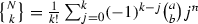 denotes the Stirling number of the second kind.
The Kolmogorov–Smirnov test statistic is 0.0127 while the critical value at the \(0,1\%\) significance level is 0.0080 for \(12 \times 10{,}000\) observations.
These numbers vary over time. The distribution of electoral votes across US states for the most recent four decades is given in “Distribution of electoral votes (Source: www.fec.gov)” section of Appendix.
Two states, Maine and Nebraska, allocate all but two of their electoral votes by Congressional district, so that a candidate needs to win a plurality of votes in a Congressional district to win that district’s electoral vote. The remaining two electoral votes (corresponding to the number of Senators in each state) are allocated to the candidate winning a plurality of the vote in the state. So, in these two states, the electoral votes may be split. I am grateful to an anonymous referee for this observation. Since neither state was considered a swing state in the 2012 election, this singularity does not affect the results of this section.
Perot in 1992 and Nader in 2000 are often cited as the most recent cases of potential “spoiler candidates”. Lee (2012) argues that third-party candidates are an integral part of the two-party system, even when they fail to win a significant percentage of votes.
See the Federal Election Commission brochure for Public Funding of Presidential Elections at http://www.fec.gov/pages/brochures/pubfund.shtml.
In the 2004 presidential election, both candidates rejected primary matching funds, but accepted public fund in the general election.
The null hypothesis that the values in \(\mathcal {V}\) are distributed according to the uniform distribution on [0, 32] cannot be rejected up to the 28% significance level based on the Kolmogorov–Smirnov test. (The p-value is 0.28.)
Had we considered the entire fifty US states and the District of Columbia (ignoring the singularities of Nebraska and Maine), the resulting combinatorial problem would also have been in the perfect phase (since \(N=51\), \(m=6\), and \(m/N =6/51 < 1\)). Indeed, a solution can readily be found by tâtonnement, as shown in “One permutation of US states satisfying Theorem 1 (2008 Electoral College)” section of Appendix, which illustrates one possible permutation of the 51 battlefields satisfying the conditions of Theorem 1.
Observe that because N is odd, given \(\kappa \) and a permutation \( \varvec{w} :=(w_1,\dots ,w_{11}) \in \mathcal {G}^*(\mathcal {V})\), there exists a unique associated vector \(\varvec{t}:=(t_1,\dots ,t_{11})\) given by (4) such that \((\varvec{t}, \varvec{w} )\) satisfies Theorem 1. Therefore, there exists a unique tangential polygon associated with each pair \((\kappa , \varvec{w} )\), \(\kappa \le \left\lfloor \frac{N-1}{2}\right\rfloor \), \( \varvec{w} \in \mathcal {G}^*(\mathcal {V})\).
See footnote 14.
Therefore, \(\left| \mathcal {G}_0( \mathcal {V})\right| =(N-1)!/2\).
The function \(\arcsin \) is defined as follows: for \(-1\le x \le 1\) and \(- \pi /2<y< \pi /2\), \(x=\sin y \Leftrightarrow y=\arcsin x\).
 ways to partition N objects into k non-empty subsets, where
  denotes the Stirling number of the second kind.
References
Arad, A., Rubinstein, A.: Multi-dimensional iterative reasoning in action: the case of the Colonel Blotto game. J. Econ. Behav. Organ. 84(2), 571–585 (2012)
Avrahami, J., Kareev, Y.: Do the weak stand a chance? Distribution of resources in a competitive environment. Cogn. Sci. 33(5), 940–950 (2009)
Barelli, P., Govindan, S., Wilson, R.: Competition for a majority. Econometrica 82(1), 271–314 (2014)
Borel, E., Ville, J.: Application de la théorie des probabilités aux jeux de hasard, original edition by Gauthier-Villars, Paris, 1938; reprinted at the end of Théorie mathématique du bridge à la portée de tous, by E. Borel & A Cheron, Editions Jacques Gabay, Paris (1938)
Borgs, C., Chayes, J., Pittel, B.: Phase transition and finite-size scaling for the integer partitioning problem. Random Struct. Algorithms 19(3–4), 247–288 (2001)
Borgs, C., Chayes, J.T., Mertens, S., Pittel, B.: Phase diagram for the constrained integer partitioning problem. Random Struct. Algorithms 24(3), 315–380 (2004)
Brams, S.J., Davis, M.D.: The 3/2’s rule in presidential campaigning. Am. Polit. Sci. Rev. 68(1), 113–134 (1974)
Brams, S.J., Davis, M.D.: Comment on ‘campaign resource allocations under the electoral college’. Am. Polit. Sci. Rev. 69(01), 155–156 (1975)
Casella, A., Laslier, J.F., Macé, A.: Democracy for polarized committees: The tale of Blotto’s lieutenants. Tech. rep, National Bureau of Economic Research (2016)
Chapman, R., Palda, K.: Assessing the influence of campaign expenditures on voting behavior with a comprehensive electoral market model. Mark. Sci. 3(3), 207–226 (1984)
Chowdhury, S.M., Kovenock, D., Sheremeta, R.M.: An experimental investigation of Colonel Blotto games. Econ. Theor. 52(3), 833–861 (2013)
Colantoni, C.S., Levesque, T.J., Ordeshook, P.C.: Campaign resource allocations under the electoral college. Am. Polit. Sci. Rev. 69(01), 141–154 (1975a)
Colantoni, C.S., Levesque, T.J., Ordeshook, P.C.: Rejoinder to ‘comment’ by S. J. Brams and M. D. Davis. Am. Polit. Sci. Rev. 69(01), 157–161 (1975b)
De Donder, P.: Majority voting solution concepts and redistributive taxation. Soc. Choice Welfare 17(4), 601–627 (2000)
Duffy, J., Matros, A.: Stochastic asymmetric Blotto games: some new results. Econ. Lett. 134, 4–8 (2015)
Duggan, J.: Equilibrium existence for zero-sum games and spatial models of elections. Games Econ. Behav. 60(1), 52–74 (2007)
Dziubiński, M.: Non-symmetric discrete General Lotto games. Int. J. Game Theory 42(4), 801–833 (2013)
Gross, O.: The symmetric Colonel Blotto game. RAND Memorandum RM-424, RAND Corporation, Santa Monica, California, (1950)
Gross, O., Wagner, R.: A continuous Colonel Blotto game. RAND Memorandum RM-408, RAND Corporation, Santa Monica, California, (1950)
Hart, S.: Discrete Colonel Blotto and General Lotto games. Int. J. Game Theory 36(3–4), 441–460 (2008)
Hart, S.: Allocation games with caps: from captain Lotto to all-pay auctions. Int. J. Game Theory 45(1–2), 37–61 (2016)
Herr, J.: The impact of campaign appearances in the 1996 election. J Politics 64(03), 904–913 (2008)
Kovenock, D., Roberson, B.: Generalizations of the General Lotto and Colonel Blotto games. ESI Working Paper 15-07, (2015)
Kvasov, D.: Contests with limited resources. J. Econ. Theory 136(1), 738–748 (2007)
Laffond, G., Laslier, J.F., Le Breton, M.: Social-choice mediators. Am. Econ. Rev. 84(2), 448–453 (1994)
Laslier, J., Picard, N.: Distributive politics and electoral competition. J. Econ. Theory 103(1), 106–130 (2002)
Laslier, J.F.: Interpretation of electoral mixed strategies. Soc. Choice Welfare 17(2), 283–292 (2000)
Laslier, J.F.: How two-party competition treats minorities. Rev. Econ. Design 7(3), 297–307 (2002)
Laslier, J.F.: Party objectives in the ‘divide a dollar’ electoral competition. In: Social Choice and Strategic Decisions, Springer, pp 113–130, (2005)
Lee, D.J.: Anticipating entry: Major party positioning and third party threat. Polit. Res. Q. 65(1), 138–150 (2012)
Levitt, S.D.: Using repeat challengers to estimate the effect of campaign spending on election outcomes in the US House. Journal of Political Economy pp 777–798, (1994)
Macdonell, S.T., Mastronardi, N.: Waging simple wars: a complete characterization of two-battlefield Blotto equilibria. Econ. Theor. 58(1), 183–216 (2012)
Montero, M., Possajennikov, A., Sefton, M., Turocy, T.L.: Majoritarian Blotto contests with asymmetric battlefields: an experiment on apex games. Econ. Theor. 61(1), 55–89 (2016)
Myerson, R.B.: Incentives to cultivate favored minorities under alternative electoral systems. American Political Science Review 87(4), 856–869 (1993)
Radić, M.: Some relations concerning k-chordal and k-tangential polygons. Math. Commun. 7(1), 21–34 (2002)
Roberson, B.: The Colonel Blotto game. Econ. Theor. 29(1), 1–24 (2006)
Roberson, B., Kvasov, D.: The non-constant-sum Colonel Blotto game. Econ. Theor. 51(2), 397–433 (2012)
Sahuguet, N., Persico, N.: Campaign spending regulation in a model of redistributive politics. Econ. Theor. 28(1), 95–124 (2006)
Schwartz, G., Loiseau, P., Sastry, S.: The heterogeneous Colonel Blotto Game. In: NETGCOOP 2014, International Conference on Network Games, Control and Optimization, October 29-31, 2014, Trento, Italy, Trento, ITALIE, http://www.eurecom.fr/publication/4479, (2014)
Snyder, J.M.: Election goals and the allocation of campaign resources. Econometrica, pp 637–660, (1989)
Szentes, B., Rosenthal, R.W.: Three-object two-bidder simultaneous auctions: chopsticks and tetrahedra. Games Econ. Behav. 44(1), 114–133 (2003)
Weinstein, J.: Two notes on the Blotto game. BE J. Theor. Econ. 12(1), (2012)
Acknowledgements
I thank three anonymous referees, Marcin Dziubiński and Balázs Szentes for helpful comments, as well as seminar audiences at UCL, Toulouse, IAS Princeton, Chapman, and the 2013 SAET conference.
Author information
Authors and Affiliations
Corresponding author
Appendix
Appendix
1.1 Bounds on \(t_n\) when N is even.
For N even, it follows from (2) that
Using (2) to express each \(t_n\) in terms of \(t_1\):
where \(b_n=\sum _{j=1}^{n}(-1)^{j+1}v_j\) for \(n=1,\dots ,N\) is defined in Corollary 2 and we use the convention \(b_0 \equiv 0\). Using (10) in (9), we obtain
Since \(b_{n}= b_{n-1}-v_n\) when n is even, and \(b_{n}= b_{n-1}+v_n\) when n is odd, the above becomes
The above system of inequalities imposes N / 2 upper bounds and N / 2 lower bounds on \(t_1\).
Condition (6) is necessary and sufficient for all N bounds to hold, and the interval in (6) defines the set of admissible values for \(t_1\). For a given \(t_1\), equation (10) uniquely defines \(t_n\) for all remaining \(n=2,\dots ,N\).
1.2 Algorithm
The following algorithm is used to build the set \(\mathcal {G}^*(\mathcal {V})\) of all permutations of the set \(\mathcal {V}\) of battlefield values satisfying Theorem 1, treating a permutation, its cyclic shifts and the order-reversing permutations of all of them as identical.Footnote 32 Fix \(\mathbf {v}:=(v_1,\dots ,v_N)\) and for each permutation \(\pi \) of \(1,\dots ,N\) let \(\mathbf {w}^\pi :=(w^\pi _1,\dots ,w^\pi _N) =(v_{\pi (1)},\dots ,v_{\pi (N)})\) denote the corresponding permutation of \(\mathbf {v}\). The existence of a tangential polygon with sides given by \(\mathbf {w}^\pi \) requires condition (2) to hold. This implies that for each \(n=1,\dots ,N\), we have \(0\le t_n\le w^\pi _{n-1}\) and \(0\le t_{n+1}\le w^\pi _{n+1}\) and therefore
Observing that this condition is harder to satisfy the larger \(w^\pi _n\), we use the following algorithm to construct \(\mathcal {G}^*(\mathcal {V})\).
-
1.
Let \(\mathcal {G}_0( \mathcal {V})\) denote the set of all possible permutations \(w^\pi \) of \(\mathbf {v}\), treating a permutation, its cyclic shifts and the order-reversing permutations of all of them as identicalFootnote 33. For each corresponding \(\pi \), let \(\tilde{n}^\pi :=\arg \max _{n\in \{1,\dots ,N\}} w^\pi _n \) denote the index of the highest valued coordinate of \(\mathbf {w}^\pi \).
-
2.
Construct the set \(\mathcal {G}_1( \mathcal {V}) \subseteq \mathcal {G}_0( \mathcal {V})\) of cyclical permutations satisfying
$$\begin{aligned} w^\pi _{\tilde{n}^\pi } \le w^\pi _{\tilde{n}^\pi -1}+w^\pi _{\tilde{n}^\pi +1}. \end{aligned}$$ -
3.
For \(k=2,\dots ,(N-1)/2\), construct the set \(\mathcal {G}_k( \mathcal {V}) \subseteq \mathcal {G}_{k-1}( \mathcal {V})\) of cyclical permutations satisfying
$$\begin{aligned} \left\{ \begin{array}{l} w^\pi _{\tilde{n}^\pi -k+1} \le w^\pi _{\tilde{n}^\pi -k}+w^\pi _{\tilde{n}^\pi -k+2},\\ w^\pi _{\tilde{n}^\pi +k-1} \le w^\pi _{ \tilde{n}^\pi +k}+w^\pi _{\tilde{n}^\pi +k-2}. \end{array} \right. \end{aligned}$$ -
4.
Eliminate from \( \mathcal {G}_ {\frac{N-1}{2}}( \mathcal {V})\) all permutations that do not satisfy (3).
The surviving permutations constitute the set \( \mathcal {G}^*( \mathcal {V})\).
Because the algorithm above exploits the conditions of Theorem 1, it does better at deriving the set \( \mathcal {G}^*( \mathcal {V})\) than the brute force method of testing all possible permutations of the elements of \(\mathcal {V}\).
1.3 Counter-example
Consider the set \(\mathcal {V}=\{1,2,3,109,110,111,325 \}\) of battlefield valuations. The set \(\mathcal {G}_1\), defined in Appendix 1, is empty, since \(325>110+111\) . Therefore, there exists no permutation of the elements of \(\mathcal {V}\) satisfying condition (2).
However, \(\mathcal {V}\) satisfies the N integer partitioning problems in Proposition 2 (ii):
\(v_n\) | partition of \(\mathcal {V}\smallsetminus \{v_n\}\) into two subsets of equal cardinality | discrepancy |
|---|---|---|
1 | \(\big \{\{109,110,111\},\{2,3,325\}\big \}\) | 0 |
2 | \(\big \{\{109,110,111\},\{1,3,325\}\big \}\) | 1 |
3 | \(\big \{\{109,110,111\},\{1,2,325\}\big \}\) | 2 |
109 | \(\big \{\{3,110,111\},\{1,2,325\}\big \}\) | 104 |
110 | \(\big \{\{3,109,111\},\{1,2,325\}\big \}\) | 105 |
111 | \(\big \{\{3,109,110\},\{1,2,325\}\big \}\) | 106 |
325 | \(\big \{\{3,109,111\},\{1,2,110\}\big \}\) | 110 |
1.4 Numerically constructing the equilibrium distribution
This section describes the method used for numerically computing the allocation of resources under \(F^*_\kappa \). Fix a given permutation \( \varvec{w} \) of the vector of battlefield values \( \varvec{v} \) such that \( \varvec{w} \in \mathcal {G}^*(\mathcal {V})\) and fix a \(\kappa \le \left\lfloor \frac{N-1}{2}\right\rfloor \). Using Mathematica, we generate 10, 000 points randomly distributed on the surface of a sphere. Each data point is then used to compute one realisation \({\varvec{x}}\) of the N-dimensional allocation vector. Recall that indices are defined modulo N. We use the notation of Sect. 3.1.
Let \(\rho _n\) denote the distance \(|O P_{n}|\) and let \(\alpha _{n}\) denote the angle \(\widehat{T_{n-1} O P_{n}}\) which by construction equals the angle \(\widehat{P_{n} O T_{n}}\) (See Fig. 9). The distance \(|O T_{n}|\) is given by the radius \(r_\kappa \) of the incircle of the tangential N-gon \({\varvec{P}}\). (In this section this radius is indexed by \(\kappa \) to emphasise the dependence.)
Consider the right triangle \( O T_{n-1} P_{n}\), where \(\widehat{T_{n-1} O P_{n}}=\alpha _n\) and where \(|O T_{n-1}|=r_\kappa \), \(|P_{n} T_{n-1}|=t_n\) and the hypotenuse is \(|O P_{n}|=\rho _n\). We have that
Since \(\alpha _{n}\) is one of the non-right apices of \( O T_{n-1} P_{n-1}\), we have that \(- \pi /2<\alpha _{n}< \pi /2\) so that \(\arcsin \left( \sin \alpha _n\right) \) is definedFootnote 34 and
Since \(\arcsin \) is strictly increasing over its domain, \(\alpha _n(r)\) is strictly decreasing in \(r_\kappa \).
Theorem 2 and Corollary 3 in Radić (2002) give the radius \(r_\kappa \) of the incirle of a \(\kappa \)-tangential polygon as an implicit function of the lengths \(t_1,\dots ,t_N\). Based on that, we obtain expressions for \(\alpha _n\) and \(\rho _n\), \(n=1,\dots ,N\).

Projecting Q onto \((P_n,P_{n+1})\)
Let \(\theta \in [0,2\pi ]\) and \(\phi \in [-\pi /2,\pi /2]\) denote the polar coordinates of R, the point uniformly distributed over the surface of the sphere \(\mathscr {S}=(O,r_\kappa )\). Let Q denote the projection of R onto the disc \((O,r_\kappa )\) inscribed in the N-gon \({\varvec{P}}\). Let \(h_n\) denote the orthogonal distance of Q from the line \((P_n,P_{n+1})\).
We orient the two-dimensional plane around the origin O by convening that \(T_1=r_\kappa e^{i0}\). We then have that
and
Moreover, since
we obtain that
and have shown in Sect. 3.1 that \(X_n=(h_n w_n)/(r_\kappa B) \sim U[0,2w_n/B]\).
1.5 Distribution of electoral votes (Source: www.fec.gov)
State | 1981–1990 | 1991–2000 | 2001–2010 | 2011–2020 |
|---|---|---|---|---|
Alabama | 9 | 9 | 9 | 9 |
Alaska | 3 | 3 | 3 | 3 |
Arizona | 7 | 8 | 10 | 11 |
Arkansas | 6 | 6 | 6 | 6 |
California | 47 | 54 | 55 | 55 |
Colorado | 8 | 8 | 9 | 9 |
Connecticut | 8 | 8 | 7 | 7 |
Delaware | 3 | 3 | 3 | 3 |
D.C | 3 | 3 | 3 | 3 |
Florida | 21 | 25 | 27 | 29 |
Georgia | 12 | 13 | 15 | 16 |
Hawaii | 4 | 4 | 4 | 4 |
Idaho | 4 | 4 | 4 | 4 |
Illinois | 24 | 22 | 21 | 20 |
Indiana | 12 | 12 | 11 | 11 |
Iowa | 8 | 7 | 7 | 6 |
Kansas | 7 | 6 | 6 | 6 |
Kentucky | 9 | 8 | 8 | 8 |
Louisiana | 10 | 9 | 9 | 8 |
Maine | 4 | 4 | 4 | 4 |
Maryland | 10 | 10 | 10 | 10 |
Massachusetts | 13 | 12 | 12 | 11 |
Michigan | 20 | 18 | 17 | 16 |
Minnesota | 10 | 10 | 10 | 10 |
Mississippi | 7 | 7 | 6 | 6 |
Missouri | 11 | 11 | 11 | 10 |
Montana | 4 | 3 | 3 | 3 |
Nebraska | 5 | 5 | 5 | 5 |
Nevada | 4 | 4 | 5 | 6 |
New Hampshire | 4 | 4 | 4 | 4 |
New Jersey | 16 | 15 | 15 | 14 |
New Mexico | 5 | 5 | 5 | 5 |
New York | 36 | 33 | 31 | 29 |
North Carolina | 13 | 14 | 15 | 15 |
North Dakota | 3 | 3 | 3 | 3 |
Ohio | 23 | 21 | 20 | 18 |
Oklahoma | 8 | 8 | 7 | 7 |
Oregon | 7 | 7 | 7 | 7 |
Pennsylvania | 25 | 23 | 21 | 20 |
Rhode Island | 4 | 4 | 4 | 4 |
South Carolina | 8 | 8 | 8 | 9 |
South Dakota | 3 | 3 | 3 | 3 |
Tennessee | 11 | 11 | 11 | 11 |
Texas | 29 | 32 | 34 | 38 |
Utah | 5 | 5 | 5 | 6 |
Vermont | 3 | 3 | 3 | 3 |
Virginia | 12 | 13 | 13 | 13 |
Washington | 10 | 11 | 11 | 12 |
West Virginia | 6 | 5 | 5 | 5 |
Wisconsin | 11 | 11 | 10 | 10 |
Wyoming | 3 | 3 | 3 | 3 |
1.6 Presidential campaign finance summaries
(Data: Federal Election Commission, Presidential Campaign Finance Summaries, http://www.fec.gov/press/bkgnd/pres_cf/pres_cf_Even.shtml)
Disbursements prior to Super Tuesday\(^\text {(i)}\) | Total disbursements | |
|---|---|---|
2012 | ||
Obama\(^*\) (D) | \({\$} 66,121,822^\dagger \) | \({\$} 469,930,646\) |
\({\$} 78,712,495^\ddagger \) | ||
Romney (R) | \({\$} 55,745,321^\dagger \) | \({\$} 298,158,415\) |
\({\$} 68,107,847^\ddagger \) | ||
2008 | ||
Obama (D) | \({\$} 115,689,084^\dagger \) | \({\$} 488,331,269\) |
\({\$} 158,579,005^\ddagger \) | ||
Mc Cain (R) (II) | \({\$} 49,650,185^\dagger \) | \({\$} 207,523,221\) |
\({\$} 58,432,608^\ddagger \) | ||
2004 | ||
Kerry (D) (II) | \({\$} 30,119,415^\dagger \) | \({\$}243,294,897 \) |
\({\$} 37,867,817^\ddagger \) | ||
Bush\(^*\) (R) (II) | \({\$} 38,901,223^\dagger \) | \({\$}286,628,893 \) |
\({\$} 46,724,159^\ddagger \) | ||
2000 | ||
Gore (D) (I) (II) | \({\$} 25,703,131^\dagger \) | \({\$} 77,863,579\) |
\({\$} 34,047,289^\ddagger \) | ||
Bush (R) (II) | \({\$} 47,964,764^\dagger \) | \({\$} 136,651,579\) |
\({\$} 60,724,475^\ddagger \) | ||
1.7 One permutation of US states satisfying Theorem 1 (2008 Electoral College)
For clarity, \(w_n\), \(t_n\) and \(t_{n+1}\) are multiplied by 538. (There are 538 electoral votes in total.)
n | \(w_n\) | \(t_n\) | \(t_{n+1}\) | n | \(w_n\) | \(t_n\) | \(t_{n+1}\) |
|---|---|---|---|---|---|---|---|
1 | 31 | 2 | 29 | 26 | 3 | 1 | 2 |
2 | 8 | 6 | 2 | 27 | 3 | 2 | 1 |
3 | 9 | 3 | 6 | 28 | 3 | 1 | 2 |
4 | 10 | 7 | 3 | 29 | 4 | 3 | 1 |
5 | 11 | 4 | 7 | 30 | 4 | 1 | 3 |
6 | 17 | 13 | 4 | 31 | 4 | 3 | 1 |
7 | 20 | 7 | 13 | 32 | 4 | 1 | 3 |
8 | 21 | 14 | 7 | 33 | 5 | 4 | 1 |
9 | 27 | 13 | 14 | 34 | 5 | 1 | 4 |
10 | 21 | 8 | 13 | 35 | 5 | 4 | 1 |
11 | 15 | 7 | 8 | 36 | 6 | 2 | 4 |
12 | 15 | 8 | 7 | 37 | 6 | 4 | 2 |
13 | 15 | 7 | 8 | 38 | 7 | 3 | 4 |
14 | 10 | 3 | 7 | 39 | 7 | 4 | 3 |
15 | 7 | 4 | 3 | 40 | 8 | 4 | 4 |
16 | 7 | 3 | 4 | 41 | 9 | 5 | 4 |
17 | 6 | 3 | 3 | 42 | 9 | 4 | 5 |
18 | 5 | 2 | 3 | 43 | 10 | 6 | 4 |
19 | 5 | 3 | 2 | 44 | 10 | 4 | 6 |
20 | 4 | 1 | 3 | 45 | 11 | 7 | 4 |
21 | 3 | 2 | 1 | 46 | 11 | 4 | 7 |
22 | 3 | 1 | 2 | 47 | 11 | 7 | 4 |
23 | 3 | 2 | 1 | 48 | 12 | 5 | 7 |
24 | 3 | 1 | 2 | 49 | 13 | 8 | 5 |
25 | 3 | 2 | 1 | 50 | 34 | 26 | 8 |
– | – | – | – | 51 | 55 | 29 | 26 |
1.8 Lorenz curves and Gini coefficients
See Tables 7 and 8 and Fig. 10.

Lorenz curves for \(\kappa =1\) in blue, \(\kappa =2\) in red, \(\kappa =3\) in green, \(\kappa =4\) in black, \(\kappa =5\) in orange
1.9 Rank and correlation properties of \(F^*_\kappa \)

Plots of the correlation matrices of \(F^*_\kappa \), for \(\kappa =1,\dots ,5\)

Plots of rank distributions under \(F^*_\kappa \) for \(\kappa =1,\dots ,5\)
Rights and permissions
About this article

Cite this article
Thomas, C. N-dimensional Blotto game with heterogeneous battlefield values. Econ Theory 65, 509–544 (2018). https://doi.org/10.1007/s00199-016-1030-z
Received:
Accepted:
Published:
Issue Date:
DOI: https://doi.org/10.1007/s00199-016-1030-z