Fundamentals of exact multi-load topology optimization – stress-based least-volume trusses (generalized Michell structures) – Part I: Plastic design

Abstract

In this two-part paper, Michell’s century-old stress-based single-load truss topology optimization paper is extended to multiple load conditions. In Part I, so-called ‘optimal plastic design’ of multi-load trusses is reviewed, which is based on ultimate (limit or collapse) load principles and requires only statical admissibility of the solution. However, its connections to ‘optimal elastic design’ will be explained, and these will be used in Part II for the full extension of Michell’s theory to elastic multi-load problems, which will fill a significant gap in our knowledge.

FormalPara Line notation

In this text, dash-dot lines denote symmetry axes, broken lines domain boundaries, dotted lines region boundaries, continuous lines with shading line supports, thick continuous lines truss members, arrows with a single thick line forces and arrows with a double line principal adjoint strains (Fig. 1).

Fig. 1

Line notation

1 Introduction – historic implications

“The undiscovered country from whose bourns ¹

No traveller returns, puzzles the will,

And makes us bear those ills we have,

Than fly to others we know not of”²

The historic implications of the present study can be explained as follows. Single-load truss topology optimization was first introduced over a century ago by Michell (1904), but nobody has extended Michell’s stress-based theory to elastic trusses with multiple loads ever since. The aim of this two-part paper is to fill this significant gap in our knowledge.

All past attempts in the literature (e.g. by Hemp, Prager and the first author) used ‘plastic design’, which has a highly limited practical applicability. Plastic design is based on a constraint on the ultimate load (collapse load) of structures having a rigid-perfectly plastic or elastic-perfectly plastic material. It requires (by the lower bound theorem of plasticity, see Section 1.1) fulfillment of the equilibrium conditions only.

On the other hand, in ‘elastic design’ we must also satisfy elastic compatibility. For a single load condition, optimal plastic and optimal elastic truss designs yield the same solution, due to statical determinacy of the optimal topology. This is not so in general for trusses with multiple load conditions. Although exact multi-load truss optimization for displacement constraints was discussed in several early papers by the first author (starting with Rozvany 1992, and Rozvany et al. 1993), and a complete theory for multi-load compliance-based truss optimization was presented this year Rozvany et al. (2014), this investigation has not been extended to stress constraints until the present study.³

Various difficulties (non-self-adjointness, static indeterminacy, non-linearity, non-convexity, non-orthogonality) have ‘puzzled the will’ of researchers, who have not produced a single exact stress-based optimal solution for an elastic truss with alternative load conditions ever since Michell’s (1904) paper. As a consequence, we had to ‘bear the ills’ of getting stuck in easier, but fairly academic problem classes like plastic optimal design. Realistic (elastic) exact multi-load truss topology optimization has remained an ‘undiscovered country’ for over a century. Well, at least until now.

Nevertheless, in this Part I we discuss mostly multi-load optimal plastic design, with a few incursions into the realm of multi-load optimal elastic design, because the former is a suitable starting point for our exploration of the latter, which is to be the subject of Part II.

1.1 The distinction between optimal elastic and optimal plastic design

As A.S.L. Chan (1960) correctly pointed out in relation to single-load studies, Hemp (e.g. 1958, 1973) tried to utilize Michell’s results in the context of ‘elastic design’, whilst Drucker and Shield (1957), and Prager (1958) applied them to ‘plastic limit design’. However, even Hemp first derived his optimality criteria for plastic design, and then showed that they are also valid for elastic design (see Section 1.1 in the book of Hemp 1973), but only for a single load condition.

In the case of Michell structures ‘elastic design’ means that the longitudinal member stresses in a linearly elastic truss may not exceed given values. In ‘plastic limit design’ or ‘ultimate load design’ an upper limit is set for the collapse load of a structure made out of a rigid-perfectly plastic or linearly elastic-perfectly plastic material.

It was shown (e.g. by Drucker et al. 1951) that for a structure having one of the above materials, a lower bound on the collapse load can be calculated on the basis of a ‘safe’, ‘statically admissible’ stress field. ‘Safe’ means that a stress field does not violate anywhere the yield condition. ‘Statically admissible’ means that a stress field satisfies static boundary conditions and equilibrium for the external forces.

A design based on the above ‘lower bound theorem of plasticity’ is called a plastic lower bound designor simply‘plastic design’. It need not take kinematic (compatibility) conditions into consideration. This is not so, however, for elastically designed trusses. It follows, therefore, that elastically and plastically designed optimal trusses are, in general, different.

1.2 Classical Michell frames for a single load condition

Fortunately, the above statement does not apply to trusses with a single load condition (and unconstrained, continuously varying member sizes), which we shall term ‘classical’ Michell structures. For those, the least-volume solution is known to be ‘statically determinate’(e.g. Sved 1954), or a convex combination of statically determinate solutions of the same minimal volume. ‘Statically determinate’ means that the internal forces can be calculated from purely statical (equilibrium) consideration and they do not depend on member sizes within a given topology.

It follows that, even for the elastic design of a ‘classical Michell truss’ (with a single load condition), the optimization can be based on statical considerations only, as in plastic design. For classical Michell trusses, therefore, optimal plastic and optimal elastic designs are identical.

This is not so, however, for generalized Michell trusses with multiple, alternative load conditions, for which the optimal plastic design is usually statically indeterminate. For multi-load trusses, therefore, we must distinguish in general between plastic and elastic optimal designs.

Classical Michell trusses are not practical, because they (a) usually have an infinite number of members, (b) ignore buckling, (c) consider one load condition only, and (d) are as a rule unstable mechanisms. However, they constitute a classical field, which has been investigated by many researchers, including some leaders in the field of structural optimization. Michell trusses are also used regularly as benchmarks for checking on the validity of various numerical methods. Moreover, the unpractical features under (c) and (d) do not apply to multi-load solutions, and the removal of the shortcoming (b) will be the subject of a future research project. However, the use of different permissible stresses in tension and compression (Rozvany 1996; Graczykowski and Lewiński 2006a, b, 2007a, b, 2010) can be regarded as a first approximation for handling the buckling problem under (b).

Important note

In this article, we use very simple examples for illustrating various general principles, so that computational complexities do not obscure fundamental properties of optimal multi-load trusses. Naturally, the same basic properties are also valid for more complicated solutions.

1.3 A brief review of the literature on classical (single load) Michell trusses

Michell’s (1904) pioneering work remained unnoticed for about half a century, after which Cox (e.g. 1958, 1965) derived some simple optimal truss layouts based on Michell’s criteria. A systematic exploration of what we now call T-regions in Michell trusses is due to Hemp (1958, 1968, 1973) and Hemp and Chan (1966) and his research associates Chan (1960) and Chan (1964, 1967a, b, 1975).

Optimal truss layouts for uniformly distributed load between supports was considered by Hemp (1974), Chan (1975), Darwich et al. (2010), Tyas et al. (2011) and Pichugin et al. (2011, 2012), and for line supports by Rozvany and Gollub (1990) and by Rozvany et al. (1997). Layouts for symmetric and unsymmetric cantilevers were studied by Lewiński et al. (1994a, b). Optimal topologies for Michell trusses with rotational restraints at both ends were derived by Rozvany et al. (1993b), and for rectangular domains with various support conditions by Lewiński et al. (1993).

Some popular Michell benchmark problems were discussed by Rozvany (1998), Lewiński and Rozvany (2007, 2008a, b) and Lewiński et al. (2013) and some general aspects of exact optimal truss layouts by Rozvany (1997) Dewhurst (2001), Dewhurst et al. (2009) and Melchers (2005).

The latest work on Michell trusses was reported by Sokół and Lewiński (2010, 2011), Lewiński et al. 2013 and by Sokół and Rozvany (2012, 2013a, c). The most recent reviews on Michell structures (Rozvany 2014a; Rozvany and Pinter 2014; Lewiński and Sokół 2014) are in a CISM volume (Rozvany and Lewiński 2014). Fundamental properties of Michell and grillage layouts were discussed by Rozvany (2011, 2014b).

Generalized Michell structures for a single load condition were considered by Rozvany et al. (1993a, 1994) for several displacement constraints, and by Rozvany and Birker (1995) for combined stress and displacement constraints.

Truss topology optimization for probabilistic (uncertain) loads was examined by Rozvany and Maute (2011), and a refutation of some unjustified allegations by Logo was presented later (Rozvany and Maute 2013a).⁴ The above example was extended to multiple load conditions by Suzuki and Haftka (2014). Truss topology optimization for elastic supports was discussed by Niu and Cheng (2014).

It is rather remarkable that in spite of so much effort and higher mathematics devoted to single-load Michell trusses, exact optimal multi-load trusses have remained a largely ‘undiscovered country’ until now.

1.4 An outline of topics discussed in this article

Optimality criteria for single load trusses on the basis of the optimal layout theory (Prager and Rozvany 1977) are reviewed in Section 2, where their extension to the plastic design of multi-load trusses is also explained. Optimality criteria for the latter are derived in the Appendix.

In Section 3 it is shown that optimal plastic design of trusses with multiple load conditions can be greatly facilitated by using superposition principles.

Based on Sections 2 and 3 above, some fundamental properties of exact multi-load trusses are outlined in Section 4.

It is shown in Section 5 that even some statically indeterminate optimal plastic designs can be utilized in optimal elastic design, if we apply a suitable prestress in some of the members.

Although this Part I of our study deals with optimal plastic design of multi-load trusses, we define classes of problems in Section 6, for which the same solutions are also optimal elastic designs.

Certain properties of multi-load optimal plastic (and elastic) designs, which enable us to derive some additional exact optimal topologies, are discussed in Section 7.

We wish to stress that in this paper we are discussing exact analytical truss optimization, which can be used for generating reliable benchmarks for numerical topology optimization. However, exact optimal truss topologies will be confirmed in this article by highly accurate numerical solutions of the second author (see Section 8).

2 Optimal plastic truss design via optimal layout theory (Prager and Rozvany 1977; Rozvany 1976)

The lower bound theorem (Drucker et al. 1951) was used by Prager and Shield (1967) for optimal plastic design. Its extension to topology optimization was discussed by Prager and Rozvany (1977), but had been applied already much earlier to flexural structures (beams, grillages frames, plates and shells), for a review see the author’s first book (Rozvany 1976).

The difference between the Prager-Shield theory of optimal plastic design and the optimal layout theory is that the latter also gives optimality conditions for ‘vanishing’ members (of zero cross-sectional area). In other words, optimal layout theory starts off with a ‘ground structure’ of all potential members, and selects the optimal ones (of non-zero cross-sectional area) out of these.

Using either one of the above theories for a single load condition, it is necessary to find

• (i) a statically admissible ‘real’ stress field for the given external loads (satisfying equilibrium and static support conditions),

• (ii) a fictitious kinematically admissible ‘adjoint’ strain field (satisfying compatibility and kinematic support conditions), such that

• (iii) the above fields fulfill certain ‘static-kinematic’ optimality criteria.

These criteria state that the adjoint strain must be a subgradient of the specific cost function for the given stress or stress resultant values. The ‘specific cost’ is the cost, weight or volume of the structure per unit length, area or volume, the specific cost function is the functional relation between the stresses or stress resultants and the specific cost. The subgradient of a function is the usual gradient in smooth regions, but at discontinuities of the gradient it is any convex combination of the adjacent gradient values.

Returning to classical Michell structures with equal permissible stress in tension and compression, we have the specific cost function (see Fig. 2a)

$$ A=k\left| F \right|,\,\,\,k=1/\sigma_{p} , $$

(1)

where A is the cross-sectional area of a truss member, F is the member force, k is a constant, and σ _p is the permissible stress in both tension and compression.

Fig. 2

a Specific cost function, b optimality criteria for Michell trusses with equal permissible stresses in tension and compression, c the relation between member forces and elastic (‘real’) strains

The adjoint strains are given by the subgradient of the specific cost function in (1),

$$ {\bar{\varepsilon}}=k\,\text{sgn}\,F\,\,\,\,\,\,(\text{for}\,\,\,F\ne 0),\,\,\,\,\,\,\left| {{\bar{\varepsilon}}} \right|\le k\,\,\,\,\,\,(\text{for}\,\,\,F=0)\,,\, $$

(2)

where ${\bar {\varepsilon }}$ is the adjoint strain (see Fig. 2b). Note that, for a zero member force, the adjoint strain is subject only to an inequality. For a comparison, the ‘real’ or elastic strains are shown in Fig. 2c. It will be seen that this is a ‘self-adjoint’ problem, because the adjoint strains are linearly proportional to the elastic strains.

For the above truss problem with a single load condition the optimality conditions arising from the layout theory reduce to those of Michell (1904).

Considering now optimal plastic truss design for several alternate load conditions equilibrated by the internal forces F _j (j = 1,2,...,m), the specific cost is subject to the inequalities

$$ A\ge k\left| {F_{j} } \right|,\thinspace (j=1,2,\,\,...\,\,m), $$

(3)

yielding the optimality condition

$$\begin{array}{@{}rcl@{}} {\bar{\varepsilon}}_{j} =\lambda_{j} k\,\text{sgn}\,F_{j} \,\,\,\,\,\,(\text{for}\,\,\,F_{j} \ne 0), \\ \left| {{\bar{\varepsilon}}_{j} } \right|\le \lambda_{j} k\,\,\,\,\,\,(\text{for}\,\,\,F_{j} = 0)\,,\, \end{array} $$

(4)

where ${\bar {\varepsilon }}_{j}$ are adjoint strains, and λ _j the Lagrange multiplier for the j-th load condition, with

$$ \lambda_{j} \ge \,0 ,\,\,\,\,\sum\limits_{j=1 }^{m} {\lambda_{j} =1 ,\,\,\,\,} \lambda_{j} >0 \,\,\,\,\text{only}\,\,\,\text{if}\,\,\,k\left| {F_{j} } \right|=A. $$

(5)

The multiplier λ _j may vary with the spatial coordinates and directions.

Proofs of the optimality conditions (4) and (5) are reviewed in the Appendix. These conditions also follow from more general relations in the author’s books (Rozvany 1976, p. 89, or Rozvany 1989, p. 47). The optimality conditions (4) and (5) can also be written in different but equivalent form (see Theorem 1 in Sokół and Rozvany 2013a).

Considering now trusses with two load conditions, if a member of non-zero cross-sectional area is fully stressed under one of the loads only, then by (4) and (5) we have

$$ \fontsize{8.8pt}{9.6pt}\selectfont \begin{array}{l} (\text{for}\thinspace\ k\left| {F_{1} } \right|=A,\,\,\,k\left| {F_{2} } \right|<A,\,\,\,F_{1} \ne 0)\,\,\,{\bar{\varepsilon}}_{1} =k\,\,sgn\,\,F_{1} ,\,\,\,{\bar{\varepsilon}}_{2} =0, \\ (\text{for}\thinspace\ k\left| {F_{2} } \right|=A,\,\,\,k\left| {F_{1} } \right|<A,\,\,\,F_{2} \ne 0\,)\,\,{\bar{\varepsilon}}_{2} =k\,\,sgn\,\,F_{2} ,\,\,\,{\bar{\varepsilon}}_{1} =0. \\ \end{array} $$

(6)

If a member is fully stressed under both loads, then (5) implies

$$ \begin{array}{l}(\mathrm{for}\,k\left| {F_{1} } \right|=k\left| {F_{2} }\right|=A,\,F_{1} \ne 0,\,F_{2} \ne 0)\ \notag\\ \bar{{\varepsilon }}_{1}=\lambda \,k\,\text{sgn}\,F_{1} , \bar{{\varepsilon }}_{2} =(1-\lambda)\,k\,\text{sgn}\,F_{2},\notag\\\text{or}\; |\overline{\varepsilon}_1|+|\overline{\varepsilon}_2| = k\end{array} $$

(7)

Finally, if a potential member has zero force in it under both loading conditions (and therefore takes on a zero cross-sectional area), then the optimality condition becomes

$$ (\text{for}\,\,\,F_{1} =F_{2} =A=0)\,\,\,\left| {{\bar{\varepsilon}}_{1} } \right|+\left| {{\bar{\varepsilon}}_{2} } \right|\le k. $$

(8)

3 Review of superposition principles for optimal plastic design considering multiple load conditions

As mentioned, optimal plastic design for multiple load conditions on the basis of (4) to (8) is rather difficult, but it can be facilitated greatly by using superposition principles.

Superposition principles for two load conditions have been proposed by Nagtegaal and Prager (1973), Spillers and Lev (1971) and Hemp (1973), and for any number of load conditions by Rozvany and Hill (1978). However, the latter is subject to certain restrictions. Here we illustrate the superposition principles with the two-load case, but use the more general expressions by Rozvany and Hill (1978).

Let the two load conditions on a truss consist of

$$ \mathbf{P}_{\mathrm{1}}=(\mathbf{P}_{\mathrm{1,1}},{\mathrm{P}}_{\mathrm{1,2}} \mathrm{,}\,\,\mathrm{...}\,\,{\mathbf{P}}_{\mathrm{1,n}})\,\mathrm{,}\,\,\,\,\,{\mathbf{P}}_{\mathrm{2}}=({\mathbf{P}}_{\mathrm{2,1}},{\mathbf{P}}_{\mathrm{2,2}}\mathrm{,}\,\,\mathrm{...}\,\,{\mathbf{P}}_{2,n}) $$

(9)

where P _j,i (j = 1,2, i = 1, ... ,n) are point loads (vectors) for the two load conditions P _j = 1,2. We define the ‘component loads’ as⁵

$$ \mathrm{\mathbf{P}}_{1}^{\ast } \,=\,(\mathrm{\mathbf{P}}_{1} +\mathrm{\mathbf{P}}_{2} )/\sqrt 2 ,\,\,\,\,\,\,\,\,\,\mathrm{\mathbf{P}}_{2}^{\ast } \,=\,(\mathrm{\mathbf{P}}_{1} -{\mathrm \mathbf{P}}_{2} )/\sqrt 2 . $$

(10)

Then the optimal plastic design for the original alternate loads can be obtained by determining the optimal designs for the component loads ${\mathrm \mathbf {P}}_{1}^{\ast } ,\,\,\mathrm {\mathbf {P}}_{2}^{\ast }$ separately, and then superimposing those two optimal designs. This means adding the cross-sectional areas $A_{1}^{\ast } ,A_{2}^{\ast }$ for the two component loads with the following scaling

$$ A=(A_{1}^{\ast } +A_{2}^{\ast } )/\sqrt 2 . $$

(11)

In (11) either of $A_{1}^{\ast } ,A_{2}^{\ast }$, or both may take on zero value.

3.1 Example in which the optimal plastic design is different from the optimal elastic design

The above procedure will be illustrated with a simple example, in which each of the two load conditions consists of a single point load (Fig. 3a and b). These are at ± 45 degrees to the horizontal, and we have a vertical line support. The correct solution to this example was briefly outlined earlier (Rozvany 1974, pp. 391-393, Rozvany and Zhou 1992, p. 100), but its full derivation is given here in detail and it is used for demonstrating several important new principles in multi-load topology optimization.

Fig. 3

Example with different optimal plastic design and optimal elastic design

Remark about the notation

Until now we used the general notation in (9) for the alternate loads. In the example that follows, we denote the magnitude (absolute value) of the single point load in both loading conditions by Q for simplicity, meaning

$$\left| {\mathrm{\mathbf{P}}_{1,1} } \right|=Q,\,\,\,\left| {\mathrm{\mathbf{P}}_{2,1} } \right|=Q. $$

The corresponding component loads given by (10) are shown in Fig. 3c and d. For these two component loads, the well known optimal topologies (e.g. Rozvany and Gollub 1990) are shown in Fig. 3e and f.⁶ These figures also show the adjoint displacements in x and y directions ${\bar {u}}_{j}^{\ast } ,\,{\bar {v}}_{j}^{\ast } \,\,(j=1,2)$ for the component loads $\mathrm {\mathbf {P}}_{1}^{\ast } ,\,\,\mathrm {{\mathbf P}}_{2}^{\ast }$.

These give (see Fig. 3e) for the first component load the principal strain of ${\bar {\varepsilon }}_{I} =k$ in the horizontal direction and zero principal strain ${\bar {\varepsilon }}_{II} =0$ in the vertical direction. The adjoint displacements for the second component load (see Fig. 3f) give the principal strains ${\bar {\varepsilon }}_{I} =-{\bar {\varepsilon }}_{II} =k$ at ± 45 degrees to the horizontal (for the derivation of this, see again e.g. Rozvany et al. (1995), p. 48, Eqs (11)). Figure 3e and f also show the cross-sectional areas of the optimal members for the component loads, which are to be superimposed to obtain the final solution for the two alternate loads.

The superimposed final topology for the original problem is shown, together with the first loading condition and the corresponding internal forces in Fig. 3g. The vector diagram for these forces is indicated in Fig. 3h. The internal forces and vector diagram for the second load condition are given in Fig. 3i and j. It can be seen that for both load conditions all members are fully stressed. The final cross-sectional areas based on (11) and the optimum volume for this optimal plastic design are shown in Fig. 3k.

It can easily be seen that the solution in Fig. 3k is not feasible in optimal elastic design. This is because for either loading case in Fig. 3g and i the two sloping members would give a zero horizontal displacement at the member intersection (Point B in Fig. 3k), but the horizontal bar would be subject to a horizontal displacement of k a/E = a/σ _p E at point B. This means that elastic compatibility is violated, and therefore optimal plastic design and optimal elastic design are different for this problem.

3.2 Proof that the optimality conditions in (4) to (8) are fulfilled by the above optimal plastic design

Although the superposition principles presented in Section 3.1 guarantee an optimal plastic design, we also check the optimality of the above example by using the original optimality criteria in (4) to (8). This will be done in two parts. First we consider adjoint strains along members of nonzero cross-sectional area, and then along vanishing members (with zero cross-sectional area).

The adjoint strain fields ${\bar {\varepsilon }}_{1} ,{\bar {\varepsilon }}_{2}$ for the original alternate loads can be calculated from the adjoint component strain fields ${\bar {\varepsilon }}_{1}^{\ast } ,{\bar {\varepsilon }}_{2}^{\ast }$ (for the component loads $\mathrm {\mathbf {P}}_{1}^{\ast } ,\,\,\mathrm {\mathbf {P}}_{2}^{\ast } )$, see Fig. 3c and d, using the relations (see Rozvany and Hill 1978)

$$ {\bar{\varepsilon}}_{1} =\frac{{\bar{\varepsilon}}_{1}^{\ast } +{\bar{\varepsilon}}_{2}^{\ast } }{2},\,\,\,\,\,{\bar{\varepsilon}}_{2} =\frac{{\bar{\varepsilon}}_{1}^{\ast } -{\bar{\varepsilon}}_{2}^{\ast } }{2}. $$

(12)

In our example, ${\bar {\varepsilon }}_{1}^{\ast } ,{\bar {\varepsilon }}_{2}^{\ast }$ can be calculated from the adjoint displacement fields ${\bar {u}}_{j}^{\ast } ,\,{\bar {v}}_{j}^{\ast } \,(j=1,2)$ in Fig. 3e and f. The adjoint strains (${\bar {\varepsilon }}_{1}^{\ast } ,{\bar {\varepsilon }}_{2}^{\ast } )$ along members of non-zero cross sectional area for the component loads are shown in Fig. 4a and b, and the adjoint strains (${\bar {\varepsilon }}_{1} ,{\bar {\varepsilon }}_{2} )$ for the original alternate loads (given by (12)) can be seen in Fig. 4c and d. Since in this problem all members are fully stressed for both loading conditions, we must use the optimality condition (7), which is completely satisfied with the multiplier values λ ₁, λ ₂ in Fig. 4e and f.

Fig. 4

a–j Check on the optimality of the solution in Fig. 3k, using the optimality criteria in (4) to (8), (k, ℓ) check on the optimal volume by dual formulation

It is more difficult to check on the optimality condition (8) for vanishing members (of zero cross sectional area), i. e. for any point and in any direction in the design domain for which there are no optimal members of non-zero cross-sectional area. In this example, the component adjoint strains and therefore the adjoint strains for the original problem, are location independent but direction dependent, i. e. ${\bar {\varepsilon }}_{1}^{\ast } (\alpha )$, ${\bar {\varepsilon }}_{2}^{\ast } (\alpha )$, ${\bar {\varepsilon }}_{1} (\alpha )$ and ${\bar {\varepsilon }}_{2} (\alpha )$ depend only on their direction (α), but not on the coordinates of their location.

The principal adjoint component strains ${\bar {\varepsilon }}_{1I}^{\ast }$, ${\bar {\varepsilon }}_{1II}^{\ast }$, ${\bar {\varepsilon }}_{2I}^{\ast }$ and ${\bar {\varepsilon }}_{2II}^{\ast }$ for ${\bar {\varepsilon }}_{1}^{\ast } ,{\bar {\varepsilon }}_{2}^{\ast }$ are shown in Fig. 4g and i, and the corresponding Mohr circles in Fig. 4h and j. It can be seen from the latter that the adjoint component strains as functions of the angle α are

$$ {\bar{\varepsilon}}_{1}^{\ast } (\alpha )=\,\,\,k(1+\cos 2\alpha )/2,\,\,\,\,{\bar{\varepsilon}}_{2}^{\ast } (\alpha )=k\cos (90^{\circ}-2\alpha )=k\sin 2\alpha . $$

(13)

Then by (12) we have

$$ \begin{array}{l} {\bar{\varepsilon}}_{1} (\alpha )=k[(1+\cos 2\alpha )/2+\sin 2\alpha ]/2, \\ {\bar{\varepsilon}}_{2} (\alpha )=k[(1+\cos 2\alpha )/2-\sin 2\alpha ]/2. \\ \end{array} $$

(14)

The curves for $\left | {{\bar {\varepsilon }}_{1} } \right |+\left | {{\bar {\varepsilon }}_{2} } \right |$ as a function of α can be seen in Fig. 5, which shows that the considered solution clearly satisfies the optimality conditions (7) and (8), with optimal member directions of −45 ^∘, 0 ^∘ and 45 ^∘ . The cusps in Fig. 5 in the $\left | {{\bar {\varepsilon }}_{1} } \right |+\left | {{\bar {\varepsilon }}_{2} } \right |$ curves occur when ${\bar {\varepsilon }}_{1}$ or ${\bar {\varepsilon }}_{2}$ take on a zero value. It can easily be shown that this occurs at α = ±arctan(1/2) = ±26.565051...°

Fig. 5

Check on the optimal topology in Fig. 3k in directions without members

3.3 Calculation of the truss volume from dual formulation

The optimal volume of trusses with multiple load conditions is given by

$$ V=\sum\limits_{i} \sum\limits_{j} \mathrm{\mathbf{P}}_{ij} {\bar{{\mathbf{\Delta }}}}_{ij} , $$

(15)

where i is the number identifying a particular point load P _{i j} within a load condition j, and ${\bar {\mathbf {\Delta }}}_{ij}$ is the adjoint displacement at the point of application of the point load P _{i j} . Within the summation we have scalar products of the point loads and the corresponding adjoint displacements.

In the example in Sections 3.1 and 3.2, we have only one point load for both loading conditions. The adjoint displacements ${\bar {\mathbf {\Delta }}}_{1} ,{\bar {\mathbf {\Delta }}}_{2}$ derived from Fig. 4c and d, and the corresponding external loads are shown in Fig. 4k and ℓ. Based on (15), the optimum volume by dual formulation is

$$ V=3akQ/\sqrt 2 , $$

(16)

as in Fig. 3k, which was based on primal formulation.

3.4 The optimal two-bar solution for the above problem (possible elastic optimal design)

In this section, we determine the optimal design within a two-bar topology. Since two-bar topologies are statically determinate, and hence kinematically admissible, they are valid for both plastic and elastic design. The solution that follows is possibly the optimal elastic design for any topology, but at present this has not been proved. Its volume is certainly an upper bound on that of the optimal elastic design.

Considering the problem in Fig. 6a, with the force diagram in Fig. 6b, the sine rule implies

$$ \frac{F_{2} }{Q}=\frac{\sin (135^{\circ}-\alpha )}{\sin (2\alpha )}. $$

(17)

Since F ₂ is the bigger member force for both load conditions, the total truss volume becomes

$$ \frac{V}{2kaQ}=\frac{\sin (135^{\circ}-\alpha )}{\cos \alpha \sin (2\alpha)}=\frac{\cos \alpha +\sin \alpha }{\sqrt 2 \sin \alpha \cos^{2}\alpha}=\frac{\sqrt 2 }{\sin 2\alpha }+\frac{1}{\sqrt 2 \cos^{2}\alpha }. $$

(18)

Then the stationarity condition d V/d α = 0 leads to

$$ 2\tan^{3}\alpha +\tan^{2}\alpha -1=0, $$

(19)

giving

$$ \alpha =33.31684^{\circ}. $$

(20)

By (18) the corresponding truss volume⁷ is

$$ V=2.5531636\;ka{\kern 1pt}Q $$

(21)

The resulting optimal topology is shown in Fig. 6c. If we optimize the truss for the same two loading conditions but for a compliance constraint, then we obtain the optimal design in Fig. 6d (see Rozvany and Zhou 1992, and Rozvany et al. 2014).

Fig. 6

a–c Optimal two-bar solution for the problem in Sections 3.1–3.3, d compliance-based optimal solution, (e- ℓ) incorrect methods for multi-load optimization

3.5 Incorrect methods for designing multi-load trusses (and other structures) by separate topology optimization for each load condition and superposition

It has been suggested that for multi-load trusses with stress constraints one of the following procedures could be used.

• (a) Worst case strategy

  • (i) Considering a given ground structure, optimize the truss separately for each loading condition. For trusses with a large number of members in the ground structure, parallel computers are recommended.

  • (ii) For any given truss member, adopt a cross sectional area, which equals the highest value for that member, out of all loading cases considered in step (i).

  It will be demonstrated on an extended version of the example in Fig. 3a and b that the above procedure can result in highly non-optimal solutions.

  In Fig. 6e to g we show three loading conditions, together with the corresponding optimal topologies considering those loads separately. The ground structure may consist of an infinite number of truss members (at all points and in all directions of the half-plane), or a finite number of members that include those three shown in Fig. 6e–g (one such ground structure is shown in broken lines in Fig. 6e).

  If we now use step (ii) above by taking the highest cross-sectional area out of Fig. 6e to g, we obtain the topology in Fig. 6h, which also indicates the volume of this design.

  We note that our correct solution (Fig. 6c) for two loading conditions does not change for the additional (horizontal) load of the magnitude 1.5 Q in Fig. 6g. This can be seen if we calculate the bar forces in the truss shown in Fig. 6c for the horizontal load of 1,5 Q. The resulting member forces are determined by means of a vector diagram in Fig. 6i.

  The stress caused by the above load in both truss members in the design in Fig. 6c is σ = F/A = 0.89750930 Q/(1.06677043 Q/σ _p )=0.841333125 σ _p , which indicates that this load condition is not active for the optimal solution in Fig. 6c (cf. Property 3 in Section 7).

  This means that the solution given by the above incorrect worst case strategy is 69.5 % heavier than the correct optimal solution. A much higher degree of non-optimality could be found by adding further load conditions.

  It is also noted that if we used the above incorrect superposition principle for the compliance-based optimal solution in Fig. 6d, then we would obtain a similarly uneconomical solution.

  We may add that the same error appears if we use a perforated plate model of high resolution and a SIMP-like algorithm (for SIMP see Bendsøe 1989, Zhou and Rozvany 1991), which result in truss-like optimal topologies for low volume fractions.

• (b) Mean value strategy

  Another erroneous suggestion is that instead of Step (ii) under Section (a) above, for any given truss member one should take the mean valueof the cross-sectional areas in single-load optimal solutions (e.g. in Fig. 6e–g). For the considered problem, this would mean that we would need to multiply the areas in Fig. 6e–g by (1/3) for each member of the combined structure in Fig. 6h, with cross-sectional areas of A = Q/3σ _p , A = Q/2σ _p , A = Q/3σ _p . It can be easily shown that such a solution would be highly non-feasible (grossly violating stress constraints).

  The absurdity of ‘averaging’ the cross-sectional areas of single load optima for multi-load optimization can be convincingly shown on a very simple example. Consider a horizontal line support, with five alternative load conditions P ₁, ... P ₅, each of which is a vertical point load of magnitude Q in a different location (see Fig. 6j, in which the second load condition is shown in continuous line, and the others in broken line). If we optimize the topology for any load condition separately, we obtain a vertical bar with a cross sectional area of Q/σ _p (see Fig. 6k). By calculating the mean value of the optimal cross-sectional areas for various load conditions, we get e.g. for the second vertical bar the mean area of (0 +Q/σ _p +0+0+0)/5=Q/5σ _p , which value is the same for all other bars (see Fig. 6 ℓ). This may appear to be an economical solution, but it is totally infeasible, because the corresponding stress in each bar for any one of the loading conditions is five times the permissible stress, σ = 5σ _p (500 % constraint violation).

  It is to be noted that the examples in this section are also valid for optimal elastic design, because the optimal topology in them is statically determinate.

3.6 Example having a statically determinate optimal plastic design, and therefore the same optimal elastic design

We shall call this example the ‘conjugate’ of the example in Section 3.1, meaning that the component loads of the previous example (Fig. 3c and d) are now the alternate loads (Fig. 7a and b), and the earlier alternate loads (Fig. 3a and b) are now the component loads (Fig. 7c and d). However, the optimal topologies are far from being the same as in the previous example.

Fig. 7

Example of a statically determinate optimal topology for two alternative load conditions

The adjoint displacement fields for the two component loads are shown in Fig. 7e and f, together with the corresponding optimal truss members.. They are both T-regions. The internal forces for the alternative loads are indicated in Fig. 7g and h, and the final cross-sectional areas given by (11) and the volume in Fig. 7i.

Since the optimal plastic design is statically determinate in this example, it is also the optimal elastic design.

4 Some fundamental properties illustrated by the above examples

The properties listed below may be self-evident for topology optimization experts, but they may not be so obvious for the non-specialist reader. The considered class of problems is ‘classical’ Michell trusses, i. e. truss volume minimization for multiple loads, equal permissible stresses in tension and compression, and continuously varying, unconstrained cross-sectional areas.

Property 1

The volume of an optimal elastic design for trusses of the considered class is greater than or equal to the optimal plastic design for the same problem.

Proof outline

The set Ξ of all elastic designs for the considered class of problems is a subset of the set π of all plastic (limit) designs, because elastic designs must satisfy all constraints for plastic design, and additional constraints representing elastic compatibility.

Then we have the following possibilities.

• (a) The optimal plastic design is unique, but it is not contained in the set Ξ of elastic designs (as in the example in Section 3.1, see also Fig. 8a).

• (b) The optimal plastic design is non-unique, but none of the plastic optimal designs of equal minimum weight are contained in the set Ξ of elastic designs (Fig. 8b).

  In both cases (a) and (b) all elastic designs in the set Ξ, including the optimal elastic design(s), have a greater volume than the optimal plastic designs, which by definition have a lower volume than any other (i. e. non-optimal) design in the set π (which also contains set Ξ).

• (c) The optimal plastic design is unique, but it is contained in the set Ξ of elastic designs (as in the example in Section 3.6, see Fig. 8c).

• (d) The optimal plastic design is non-unique but some optimal plastic designs are contained in the set Ξ of elastic designs (Fig. 8d).

  Fig. 8

  

  Proof of Property 1

  In both cases (c) and (d) some of the optimal plastic designs are also optimal elastic designs, and therefore both optimal plastic and optimal elastic designs have the same minimum volume.

Property 2

If an optimal plastic design is statically determinate, then it is also the optimal elastic design.

Proof outline

In an optimal elastic design, the compatibility of the deformations must also be fulfilled. However, in a statically determinate optimal plastic design the deformations are always compatible, and therefore they are also optimal elastic designs.

5 Conversion of optimal plastic design into optimal prestressed elastic design, a generalization of the first author’s ‘reversed deformation method’

5.1 Trusses with a single load condition

The so-called ‘reversed deformation method’ (Rozvany 1964), was illustrated with examples of arch-bridges, pressure vessels and beam systems (grillages), but here we discuss it in the context of trusses. We can use basically the following procedure for any linearly or nonlinearly elastic truss with a single load condition.

• (1) Divide the structure into statically determinate sub-systems by applying ‘cuts’ at suitable locations. For trusses these cuts are usually at joints (i. e. points of member intersections).

• (2) For each sub-system assign forces (termed ‘connection forces’) at the cuts such that they are in equilibrium (i) with similar forces for the other sub-systems at a particular cut, and (ii) also within each subsystem, including external loads (this is equivalent to plastic design as described previously).

• (3) Assign member sizes to each subsystem, such that under the combined effect of external loads and connection forces all members are fully stressed (reach the permissible stress) in any of the sub-systems.

• (4) Calculate the relative displacements at the cuts of each statically determinate sub-system for the external load and the above described connection forces.

• (5) The manufactured initial shape of each sub-system is obtained by using the negative value of the above displacements (i.e. ‘reversed deformations’).

At the fabrication stage, there will be a lack of fit between the sub-systems of the structure, and these are eliminated by prestressing (‘pulling the cut parts together’). This will cause certain deformations in the assembled structure. However, at the given external loading, the elastic deformations and the manufactured reversed deformations cancel out, and the cuts will be subject to zero displacements.

In an extended version of this method, we can synthesize a prestressed structure for some prescribed non-zero displacements.

In optimal prestressed elastic design, in step (2) above we select the statically admissible connection forces optimally.

Note

Classical Michell frames are statically determinate (or convex combinations of statically determinate solutions) for a single load conditions. However, other structures (e.g. generalized Michell structures with prescribed minimal cross-sections) are often statically indeterminate even for a single load condition. This is particularly so for non-self-adjoint problems (in which the ‘real’ and ‘adjoint’ strains are not proportional to each other).

5.1.1 An elementary example of statically indeterminate optimal plastic truss design for a single load condition, made into an optimal prestressed elastic design by the reversed deformation method

Consider the elementary two bar truss with a point load Q = 4B/k in the middle (Fig. 9a), where B is the prescribed minimum cross-sectional area for the truss members. The specific cost function for this problem is shown in Fig. 9b. It can be seen that we have different permissible stresses in compression and tension, with σ _C = 1/k, σ _T = 2/k.

• (a) Optimal plastic design. Using the optimal layout theory (Prager and Rozvany 1977), optimal adjoint strains ${\bar {\varepsilon }}$ are given by the sub-gradients of the specific cost function, which are shown in Fig. 9c. This problem is not self-adjoint, the real elastic strains ε for various values of the member force F are shown in Fig. 9d (where E is the same Young’s modulus in tension and compression).

  Fig. 9

  

  Statically indeterminate optimal plastic design converted into prestressed optimal elastic design

  The statically admissible member forces in the optimal plastic design are shown in Fig. 9e, for which the adjoint strains in Fig. 9f satisfy (i) compatibility, and (ii) the optimality condition represented graphically in Fig. 9c. Note that at F = −B/k the adjoint strain in Fig. 9c is non-unique).

  The cross-sectional areas based on the forces in Fig. 9e divided by the corresponding permissible stresses are shown in Fig. 9h, and give a volume of V = 2.5aB for optimal plastic design.

• (b) Optimal prestressed elastic design by reversed deformations. The member forces in Fig. 9e would give the elastic strains in Fig. 9g. These elastic strains cause different elongations in the two members, namely 2a/kE in the top member and –a/kE in the bottom member. Hence they are kinematically inadmissible for elastic design.

  However, this can be corrected by suitable prestress, namely by manufacturing the top member 2a/kE shorter and the bottom member a/kE longer than their planned length and using prestress to close in the lack of fit. Then the combined elongations due to lack of fit and the given external force would add up to zero, resulting in (i) elastic compatibility and (ii) zero displacement at the loaded point (Point C in Fig. 9a).

5.1.2 Optimal elastic design (without prestress) for the problem in Section 5.1.1

Statically admissible forces in the above problem are shown in Fig. 10a. Assuming that the lower bar develops the permissible stress in compression (σ _C = 1/k), we have the cross-sectional area for the bottom bar

$$ A_{2} =(Q-F_{1} )k=(4B/k-F_{1} )k, $$

(22)

causing an elastic strain of

$$ -\frac{1/k}{E}=-\frac{\sigma_{C} }{E} $$

(23)

in the bottom bar.

Fig. 10

Optimal elastic design without prestress for the problem in Fig. 9

The top bar could develop a twice as high (σ _T = 2σ _C ) stress, but this is not admissible kinematically, because the elastic elongation of the two bars must have the same absolute value. This is only possible if the cross-sectional area of the top bar is

$$ A_{1} =F_{1} k. $$

(24)

A fully stressed top bar is not feasible, because then the bottom bar would also need to have the same elongation and therefore the same stress as the top bar, but such a stress would exceed the permissible stress in compression (by factor two). Moreover, both cross-sectional areas must be greater than their prescribed minimum value B. The resulting non-unique optimal area values that satisfy (22) and (24) are shown in Fig. 10b.

The corresponding optimal elastic truss volume is

$$ V=a[(4B/k-F_{1} )k+ F_{1} k]=4aB, $$

(25)

which is 60 % higher than the volume of the optimal plastic design (or of the optimal prestressed elastic design) in Fig. 9h. This shows that prestressing could be economically justified in some design problems.

The optimal elastic design is non-unique because we may have any cross-sectional areas satisfying A ₁≥B, A ₂≥B, as well as (22) and (24). The limiting cases are shown in Fig. 10c–f.

5.2 Optimal prestressed elastic design for multiple load conditions

It will be demonstrated on examples that the lack of elastic compatibility in an optimal plastic design for multiple loads can be easily eliminated by prestressing, if there exists a set of redundant members that has the same member force for all load conditions. A ‘set of redundant members’ means a set of members, whose removal renders the structure (i) statically determinate, but (ii) stable.

• Example (a): Making the optimal plastic design in Section 3.1 kinematically admissible by prestressing. Considering again the problem in Section 3.1, the elastic strains (as distinct from adjoint strains) in the members for the load P ₁ in Fig. 3a can be calculated from the internal forces in Fig. 3g and cross-sectional areas in Fig. 3k. They are shown in Fig. 11a (all members are fully stressed). For the two sloping members this would result in the displacements in Fig. 11b (with zero horizontal resultant displacement), and for the horizontal member we would have a horizontal displacement only (Fig. 11c). As noted before, the two displacements are incompatible, and therefore this solution cannot be an elastic optimal design.

  Fig. 11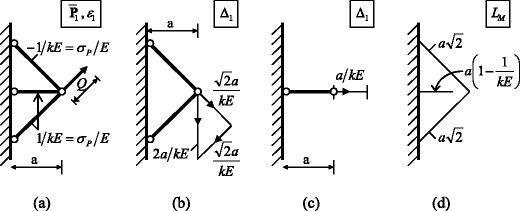

  

  Prestressed elastic version of the plastic optimal design in Fig. 3k

  However, using the reversed deformation method, the manufactured lengths (L _M ) shown in Fig. 11d restore compatibility with fully stressed members. For the second load condition, the structure is also compatible and fully stressed for the same prestressing.

  Comparing the volume values in Fig. 3k (optimal plastic design or optimal prestressed elastic design)and in (21) (possible optimal elastic design without prestress), it can be concluded that prestressing would result in over 20 % volume saving in this case.

• Example (b): Five-bar truss. The alternative load conditions for this problem are shown in Fig. 12a and b, and the component loads, together with the corresponding optimal designs in Fig. 12c and d. The latter can be easily derived from similar solutions in the paper by Rozvany and Gollub (1990). The final optimal plastic design based on superposition principles (Section 3) is shown in Fig. 12e. It can be easily shown that this design does not fulfill elastic compatibility conditions. If we considered only the four sloping members, then we would obtain the same vertical displacement for the member intersections C and D in Fig. 12e. However, the vertical member between points C and D has an elastic elongation of a/kE. Compatibility can be restored if the manufactured length of the vertical bar is a(1−1/kE).

  Fig. 12

  

  Prestressed elastic optimal design consisting of a five-bar truss

• Example (c) Michell cantilever for two load conditions. Here we consider trusses within a rectangular domain whose boundaries are indicated in broken lines. Again, the alternative loads are shown in Fig. 13a and b, and the component loads together with the corresponding optimal designs in Fig. 13c and d. The resulting final design for the original alternative loads, which is clearly kinematically inadmissible, can be seen in Fig. 13e. To restore elastic compatibility, we must again use a fabricated length of a(1−1/kE) for the bar CD.

  Fig. 13

  

  Prestressed elastic Michell cantilever for two load conditions

6 Classes of multi-load truss topology optimization problems for which the optimal plastic design is also optimal elastic design

In this section we outline some classes of multi-load problems, for which the optimal plastic design is always statically determinate, and hence it is also an optimal elastic design.

6.1 Symmetric topologies with loads along the axis of symmetry and principal adjoint strains at 45 degrees to the axis

This class of problems can be defined as follows.

• (i) The support conditions and the domain boundaries are symmetrical.

• (ii) The alternate loads consist of point loads acting along the axis of symmetry.

• (iii) All the forces in the component loads are either (a) normal to the axis of symmetry and are pointing in the same direction, or (b) do not deviate from the normal of the axis of symmetry by more than ± 45 degrees.

• (iv) In the adjoint strain field for the component loads, there are T-regions along the axis of symmetry with principal adjoint strains at 45 degrees to that axis.

An example fulfilling conditions (i) and (iv) (a ‘Michell cantilever’, actually derived fully by Lewiński et al. 1994a) is shown in Fig. 14a.

Fig. 14

Optimal plastic and elastic truss topologies for loads along the axis of symmetry

Figure 14a also shows some possible component loads, and it can be seen in Fig. 14b that the point loads in each component load could be inclined by up to ± 45 degrees to the vertical (see the above paper).

Figure 14c and d show alternate loads for which the component loads (Fig. 14e and f) fulfill the requirements in Fig. 14b. The component loads are not yet divided by $\sqrt 2$ in order to make it easier to understand the construction.

Since the final design under the above conditions is a ‘Michell cantilever’ (Fig. 14a), it is statically determinate. This topology is equally optimal in plastic and elastic design.

Important remark

The problem in Section 3.6 is a special case of the problems considered in this section, actually the borderline case with the component loads at ± 45 degrees to the normal of the symmetry axis.

6.2 Skew-symmetric problems with loads along the axis of symmetry

In a skew symmetric problem, the supports and domain boundary are symmetric and the loads skew-symmetric. We consider the special case when (a) concentrated loads act along the axis of symmetry and they are normal to the axis, and (b) at each loaded point the ratio of the alternative loads (and therefore the ratio of the component loads) is the same.

It was shown elsewhere (Rozvany 2011) that for a skew symmetric problem of a certain class (e.g. Michell trusses) at least one optimal layout is symmetric, and the internal forces in it skew-symmetric. In a multi-load truss problem with all the alternate loads normal to the axis of symmetry, the component loads will also be normal to the axis.

For both component loads the symmetric optimal layout is the same (only the cross-sectional areas are different), so the final layout is also the same. If we superimpose two or more statically determinate designs of the same layout, then the resulting design will also be statically determinate. Hence for the above class of problems the optimal plastic and elastic designs are the same.

The above conclusions are illustrated in Fig. 15 with a simple example, which was derived by Michell (1904). This problem is not the type described under Section 6.1, because at the point load the principal adjoint strains are partially non-unique (within the fans), violating Condition (iv). However, for vertical alternate loads (Fig. 15b and c) the component loads are also vertical (in Fig. 15d and e multiplied by $\sqrt 2 )$, and therefore the optimal layout is statically determinate for the final solution. Using the extended superposition principles (Rozvany and Hill 1978), this conclusion can also be generalized to any number of load conditions.

Fig. 15

Optimal topology for a skew-symmetric problem with two load conditions (modified problem of Michell (1904))

6.3 The external forces in the component loads are distant enough to prevent interaction

• Example (a). Two alternate loads in opposite directions. In Fig. 16a and b the alternate point loads are too far apart to ‘help each other’ in reducing the truss volume. The component loads, together with the optimal regions and the forces in the optimal truss members are shown in Fig. 16c and d, and the final optimal design in Fig. 16e. It can be seen that the structure is statically determinate, and therefore it is valid for both plastic and elastic optimal design. For the explanation of the optimal regions in Fig. 16c and d see the texts by Rozvany and Gollub (1990) or Rozvany et al. (1995), p. 48.Important note If the distance between the point loads in in Fig. 16a and b were smaller than 4a, then we would have a connecting horizontal bar between points C and D, and the design would be statically indeterminate (see e.g. Fig. 12, in which the line support is vertical, i. e. the problem in Fig. 16 is turned around by 90 degrees).

  Fig. 16

  

  Example with two collinear loads without interaction

• Example (b). Two alternative loads at right angles. In Fig. 17a and b we show the alternative loads, and in Fig. 17c and d the component loads, optimal regions and optimal member layouts. In Fig. 17c the adjoint displacements are also given in full for the first component load, for the other component load in Fig. 17d the adjoint displacements are similar with some sign differences. The optimal superimposed cross sectional areas are shown in Fig. 17e.

  Fig. 17

  

  Example with two loads at right angles, no interaction

  It can be seen that there is no interaction between the two alternative loads in this problem.

7 Additional properties of multi-load optimal plastic (and elastic) trusses, which can be used for deriving optimal topologies

Property 3

Let a truss design (i.e. layout and cross-sectional areas) be an optimal plastic design for the load conditions 1, 2, ... , g. Then the same truss is an optimal plastic design for the load conditions 1, 2, ... , g, ... , m, if for the load conditions g + 1, g + 2, ... , m there exist statically admissible member forces, for which the stresses do not exceed their permissible values.

Definition 1

‘Feasible’ solutions shall mean those that are statically admissible and do not violate stress constraints for any of the load conditions..

Proof

Θ_1,2,...,g , Θ _{g+1,g+2,...,m} and Θ_1,2,...,m will denote the sets of feasible solutions for the load conditions: 1, 2,... , g; g+1, g+1, ... , m; and 1, 2, ... , m, respectively (see Fig. 18). If the solution represented by point Z is optimal for Θ_1,2,...,g and additionally Z∈Θ _{g+1,g+2,…,m} , then it is also optimal for (Θ_1,2,...,g ∩Θ _{g+1,g+2,...,m} )⊂Θ_1,2,...,g , because an optimal solution for a given set is always optimal also for a subset of that set, provided that such solution is contained in that subset.

Fig. 18

Proof of Property 3

Example 1 (Statically determinate solution)

Optimize the truss topology for the load conditions P ₁ to P ₄ shown in Fig. 19a, with the cost factor k = 1 (unit permissible stress in tension and compression). In order to invoke Property 3 (with g = 1), we first determine the optimal topology for the load condition P ₁, for which the well-known solution is shown in Fig. 19b, with the optimal cross-sectional areas in Fig. 19c. Then we check that the permissible stress is not exceeded for the load conditions P ₂ to P ₄, see Fig. 19d to f. It follows therefore from Property 3 that the design in Fig. 19c is optimal for the alternative load conditions P ₁ to P ₄.

Fig. 19

Application of Property 3 in obtaining a statically determinate optimal topology for four load conditions

Remark 1

The design in Fig. 19c is also optimal for forces P ₁ to P ₄ of smaller absolute values than the ones indicated in Fig. 19a, in fact optimality is preserved if these forces point in the opposite direction.

Remark 2

Since the optimal design in Fig. 19c is statically determinate, it is also an optimal elastic design for the alternative load conditions in Fig. 19a. This is noteworthy because the authors do not know of any other non-trivial elastic optimal truss design for four load conditions.

Example 2 (Statically indeterminate solution)

Optimize a generalized Michell truss for the four alternative load conditions (P ₁ to P ₄) in Fig. 20a. We will start first with the optimal topology for the two load conditions (P ₁ and P ₂) in Fig. 20b, which is shown in Fig. 20c (cross-sectional areas also indicated). This is actually the same solution as the one derived in Section 3.1, Fig. 2k, but with the specific values of k = 1 and $Q =\sqrt 2$.

Fig. 20

Application of Property 3 in obtaining a statically indeterminate optimal topology for four load conditions

If we now consider the two other loading conditions (P ₃ and P ₄ in Fig. 20a), it can be seen from Fig. 20d and e that for the same truss topology there exist statically admissible bar forces, for which the stresses do not exceed the permissible values. By Property 3 above, therefore, the same plastic truss design is optimal for the four alternative load conditions in Fig. 20a.

It can be seen from Fig. 20f, that the above topology remains optimal, if we increase the magnitude of the horizontal force (i.e. P ₃) up to a value of 2.0. For the limiting case with a horizontal force of 2.0, the internal forces satisfying the stress constraints are shown in Fig. 20f. For greater values of P ₃ and the topology in Fig. 20c, we cannot find statically admissible member forces within the stress constraints, and therefore the optimal topology changes. The optimal design for the four alternative loads in Fig. 20g (with |P ₃| = 3) is in 20h, this was derived numerically by the second author (see Section 8).

Example 3 (Unequal permissible stresses in tension and compression)

Determine the optimal truss topology for the two alternative load conditions in Fig. 21a and b, if the permissible stresses, and the corresponding cost factors in tension and compression are

$$ \sigma_{T} =1,\,\,\,\sigma_{C} =1/3,\,\,\,k_{T} =1,\,\,\,k_{C} =3. $$

(26)

For different permissible stress values in tension and compression, the optimality conditions in (2) change to (see Rozvany 1996)

$$ {\begin{array}{*{20}c} {{\bar{\varepsilon}}=-1/\sigma_{C} } & {(for\;\;F<0),} \\ {{\bar{\varepsilon}}=1/\sigma_{T} } & {(for\;\;F>0),} \\ {-1/\sigma_{C} \le {\bar{\varepsilon}}\le 1/\sigma_{T} } & {(for\;\;F=0),} \\ \end{array} } $$

(27)

in which the inequality implies that in the optimal truss topology the members must run in the principal directions of the adjoint strain field.

Fig. 21

Application of Property 3 in obtaining an optimal topology for four load conditions and different permissible stresses in tension and compression

If we have a T-region (with members running in two directions), then by (26) and (27) the principal adjoint strains are

$$ {\bar{\varepsilon}}_{1} =1,\,\,\,{\bar{\varepsilon}}_{2} =-3. $$

(28)

First we optimize the truss topology for the first loading condition P ₁, by a somewhat modified version of derivation by Rozvany and Gollub (1990). The adjoint displacements in the x and y directions for the optimal topology are given by (see Fig. 21c)

$$ {\bar{u}}=-2x,\,\,\,\,{\bar{v}}=2\sqrt 3 x $$

(29)

implying

$$ {\bar{\varepsilon}}_{x} =\frac{\partial {\bar{u}}}{\partial x}=-2,\,\,\,{\bar{\varepsilon}}_{y} =\frac{\partial {\bar{v}}}{\partial y}=0,\,\,\,{\bar{\gamma}}_{xy} =\frac{\partial {\bar{u}}}{\partial y}+\frac{\partial {\bar{v}}}{\partial x}=2\sqrt 3 . $$

(30)

Then the Mohr circle in Fig. 21d shows that the principal strains for the adjoint strains in (30) are the ones in (28), and the angle between the axis x and the principal directions is 30 ^∘ and 60 ^∘. Using bars in the above principal directions, we obtain the optimal topology in Fig. 21c, with the statically admissible forces given by the vector diagram in Fig. 21e. Dividing these forces by the corresponding permissible stresses, we get the optimal cross sectional areas in Fig. 21f, and the optimum truss volume of $V=2\sqrt 3$. The latter can be confirmed by dual formulation, using the vertical displacement in (29) for the dual formula in (15).

With a view to using Property 3 above, we now check the stresses for the second alternative load condition P ₂ (i.e. for the horizontal load with the magnitude 1.5). This is balanced by the bar forces shown in Fig. 21g. Dividing these by the cross sectional areas in Fig. 21f, we obtain the stresses in Fig. 21h. Since for this load condition both bars are in tension, the permissible stress for both bars is ${\bar {\varepsilon }}_{1} =1,$ and the stress for the second load condition is $\sqrt {3/2} =0.866...$. Then by Property 3 the optimal topology in Fig. 21c is valid for the two alternative load conditions in Fig. 21a and b.

It is to be remarked that if we increased the magnitude of the horizontal force to $\sqrt 3 =1.732...$, then the corresponding stresses in the two members would become unity, and the optimal topology in Fig. 21c would be still valid, with both bars fully stressed for both load conditions. Similarly, if the load condition P ₂ consisted of a horizontal force of $1/\sqrt 3$ (or smaller) in the opposite direction (from right to left), then we would have compressive stresses of 1/3 or less in both bars, and the solution in Fig. 21c would again be valid (the stresses for the second load condition being less than or equal to the permissible stresses).

Since the optimal topology is statically determinate in this case, it is also valid for optimal elastic design.

Note

Property 3 may look self-evident and procedures based on it may seem trivial, but it entails some difficulties. We first have to find a set of load condition(s), the optimal topology for which makes all other load conditions inactive. Considering the above example, if we started with the second load condition P ₂, we would obtain the optimal topology in Fig. 21i, which could not transmit the load in P ₁, making that load infeasible. Moreover, we must determine the optimal topology for the active load conditions, which can be a rather challenging task.

A more specific consequence of Property 3 can be formulated as follows.

Property 4

Let a given truss be an optimal plastic design for the load conditions 1, 2, ... , g. Then the same truss is an optimal plastic design for the load conditions 1, 2, ... , g, ... , m, if the load conditions g+1, g+2, ... m are the convex combinations of conditions 1, 2, ... , g.

Proof

Let P _l be the new load condition composed of the convex combination of conditions 1, 2, ... , g:

$$ \mathrm{\mathbf{P}}_{l} =\sum\limits_{j=1}^{g} {\alpha_{j} \mathrm{\mathbf{P}}_{j} } ,\;\;\;\text{where}\;\;\sum\limits_{j=1}^{g} {\alpha_{j} } =1\;\;\text{and}\;\;\alpha_{j} \ge 0. $$

(31)

Then the member forces

$$ \mathrm{\mathbf{F}}_{l} =\sum\limits_{j=1}^{g} {\alpha_{j} \mathrm{\mathbf{F}}_{j} } $$

(32)

satisfy the equilibrium equations for the new load condition (31). Moreover, for any bar (e) the two inequalities hold

$$ F_{e,l} /\sigma_{T} =\sum\limits_{j=1}^{g} {\alpha_{j} F_{e,j} /\sigma_{T} } \le A_{e} \sum\limits_{j=1}^{g} {\alpha_{j} } =A_{e} $$

(33)

and

$$ -F_{e,l} /\sigma_{C} =-\sum\limits_{j=1}^{g} {\alpha_{j} F_{e,j} /\sigma_{C} } \le A_{e} \sum\limits_{j=1}^{g} {\alpha_{j} } =A_{e} $$

(34)

Thus the permissible stress constraints are also satisfied and hence the forces defined by (32) are statically admissible. According to Property 3, the optimal truss for conditions 1, 2, ... , g is still optimal for conditions 1, 2, ... , g and l.

Example 4 (Infinite number of load conditions)

Optimize the truss topology for the infinite number of load conditions defined as any linear-convex combination of P ₁ and P ₂ (see Fig. 22a). Assume the cost factor k = 1 (unit permissible stress in tension and compression).

Fig. 22

Application of Property 4 for infinite number of load conditions

Based on the previous considerations, we know that for two load conditions P ₁ and P ₂ the optimal solution is the two-bar truss (see Fig. 7). The member forces for these load conditions are presented in Fig. 7g and h. Using the superposition principle, it is easy to obtain the member forces for any new load condition, defined by P _j = λ P ₁+(1−λ)P ₂, 0 ≤ λ ≤ 1. These forces are presented in Fig. 22b. Note that the member force in the bottom bar is constant while the force in the top bar varies from $-Q/\sqrt 2$ to $Q/\sqrt 2$. However, the maximal absolute value of these forces does not exceed $Q/\sqrt 2$, hence the cross-sectional areas shown in Fig. 22c are large enough to carry any new load condition P _j . In other words no additional volume of material is needed.

8 Numerical check on some of the exact multi-load optimal topologies

The analytical solutions presented in the previous sections have been confirmed numerically using the adaptive ground structure method and the software recently developed by the second author (Sokół and Rozvany 2013b). This software uses a previously written and tested code (Sokół 2011a, b) and its natural extension to stress-based multi-load case problems. A similar method was proposed by Gilbert and Tyas (2003). The above algorithm makes use of both active set and interior point methods and allows us to solve large-scale optimization problems (see Sokół and Rozvany 2013b for more implementation details).

The numerical solutions of the problems in Figs. 3, 7, 12, 16, 17, 19, 20 (including h), 21 ⁸ and 22 are identical with the exact analytical solutions, giving the same optimal layouts and volumes (thus no new figures are needed here). In order to verify the results for each problem, the calculations were performed using several different densities of the ground structure.

From a numerical point of view, the most interesting results were obtained for the problems in Figs. 13 and 14. The numerical solution of the first of these problems is presented in Fig. 23. It was carried out using the ground structure composed of 100×50 cells and 8 067 890 potential bars, giving the layout predicted in Fig. 13e with the volume V _{n u m} , which is only 0.1 % greater than the exact optimal volume V _a . The latter is the sum of the volume of the straight vertical bar V _b and the volume V _c of two truss-like cantilevers. The exact value of V _c can be derived after Lewiński et al. (1994a). Its accurate numerical approximation can also be found in Graczykowski and Lewiński (2010, see Table 2 for x = 2a and y = 0.5a).

Fig. 23

Numerical confirmation of the analytical solution of the problem of Fig. 13

Figure 24 presents the numerical solution of the two-load case problem defined in Fig. 14a for selected slopes of P ₁ and P ₂ and for arbitrary assumed five points loads for every load condition. The exact analytical solution for the present problem can also be obtained using the formulas derived in Lewiński et al. (1994a) but this laborious task is omitted here. The main purpose of this calculation was to check whether the layout predicted in Fig. 14a is correct, and one can easily see that it is. Note that the layout is symmetric but the cross-sectional areas in upper and lower bars are different. The result presented in Fig. 24 was obtained using the ground structure composed of 150×50 cells and 18 031 172 potential bars.

Fig. 24

Numerical solution of the problem of Fig. 13

Finally, it is worth noting that numerical solutions based on the adaptive ground structure approach are much easier to obtain than analytical solutions, and give very accurate approximations of exact solutions (for adequately dense grids). Furthermore, and contrary to analytical methods, numerical solution can easily be obtained for any supports and load conditions. For example, the exact analytical solution to the modified problem of Fig. 17 with b = a is not yet known, but it does not present any additional difficulty in obtaining a numerical solution (see Fig. 25), which can serve as a valuable hint for obtaining a new exact solution. Obviously, the volume V _{n u m} = 2.66132akQ is less than 3akQ of the three-bar solution presented in Fig. 17e. It was checked in several numerical tests that the three-bar solution is optimal for b≥ 2a. For b < 2a the optimal truss is more complicated and consists of one circular fan and five straight bars (Fig. 25).

Fig. 25

Optimal topology of the modified problem of Fig. 17

However, the advantage of exact analytical solutions is that they often cover an entire class of problems, and provide a deeper insight into fundamental properties of optimal structural topologies. Moreover, numerical solutions do not help much at present in determining the adjoint strain field in so-called O-regions (regions without members). Also, exact solutions are the most reliable and most accurate means of checking on the validity, accuracy and convergence of numerical methods.

9 Concluding remarks

In Part I of this study, we discussed plastically designed multi-load least-volume trusses, and their relevance for elastically designed optimal trusses. The latter will be examined in detail in Part II of this two-part paper.

Appendix: Proof of optimality criteria for multi-load trusses – plastic design

For simplicity, we derive these optimality conditions for ground structures with a finite number of members (e = 1, 2, ..., E), but the results can easily be extended to an infinite number of members by using variational methods (Rozvany 1976, 1989). However, even the finite formulation is valid for ground structures with an arbitrarily large number of members, and therefore it should be sufficient for all practical purposes.

The problem can be stated as

$$ \min \,\,\,V=\sum\limits_{e=1}^{E} {A_{e} \,L_{e} } , $$

(A1)

subject to

$$ A_{e} \ge k\left| {F_{e,j}^{\mathrm{s}} } \right| ~\,\,(e=1,\thinspace 2,\thinspace ...\thinspace , E,\,\,\,j=1,2,\,\,...\,\,m), $$

(A2)

in which V is the truss volume, A _e and L _e are the cross-sectional area and length of the e-th truss element, k = 1/σ _p , where σ _p is the permissible stress in both tension and compression, and $F_{e,j}^{\mathrm {s}}$ is the statically admissible force in the eth truss element for the jth load condition.

The derivation that follows is an extension to multiple loads of the proof by Rozvany (1996, Section 6.2, p. 247), but the method based on slack variables is similar to that of Hemp (e.g. 1973).

Fig. 26

The role of slack variables in the proof of optimality criteria for multi-load plastic truss design

The inequality in relation (A2) can be replaced by the equalities

$$ A_{e} =kF_{e,j} +s_{e,j}^{+2}\,,\,\,\,A_{e} =-kF_{e,j} +s_{e,j}^{-2}, $$

(A3)

where $s_{e,j}^{+} \;\text {and}\;s_{e,j}^{-}$ are slack variables (see Fig. 26, in which lines with a short shading denote inequalities. The shaded area at the top denotes feasible values for A _e and F _e,j ). The equilibrium requirement for the member forces F _e,j (e = 1, 2, ... ,E, j = 1,2, ... m) and external forces P _i,j (i = 1,2, ... ,n), (j = 1,2, ..., m) can be expressed conveniently by using the virtual displacements principle (Argyris and Kelsey 1960)

$$ \sum\limits_{i=1}^{n} {\bar{\text{\textbf{u}}}_{i,j}^{\mathrm{k}} \mathrm{{\mathbf P}}_{i,j}^{\mathrm{s}} =\sum\limits_{e=1}^{m} {{\bar{\varepsilon}}_{i,j}^{\mathrm{k}} } } L_{e} F_{i,j}^{\mathrm{s}} \,\,\,(j=1,2,\,\,...\,\,m), $$

(A4)

where ${\bar {\text {\textbf {u}}}}_{i,j}^{\mathrm {k}}$ (vectors) is a virtual displacement at the point of application of the external force $\mathrm {{\mathbf P}}_{i,j}^{\mathrm {s}}$, and ${\bar {\varepsilon }}_{e,j}^{\mathrm {k}}$ is a virtual strain in the e-th truss element for the j-th load condition. The superscripts k indicate that ${\bar {\text {\textbf {u}}}}_{i,j}^{\mathrm {k}}$ and ${\bar {\varepsilon }}_{e,j}^{\mathrm {k}}$ must be kinematically admissible (compatible). The superscripts s indicates that $\mathrm {{\mathbf P}}_{i,j}^{\mathrm {s}}$ and $F_{e,j}^{\mathrm {s}}$ must be statically admissible (in equilibrium with each other).

Then the augmented (Lagrange) function can be stated as

$$\begin{array}{@{}rcl@{}} &&\hat{{V}}=\sum\limits_{e=1}^{E} {\left\{ {A_{e} +\sum\limits_{j=1}^{m} {\left[ {\upsilon_{e,j}^{+} (kF_{e,j}^{s} +s_{e,j}^{+2}-A_{e} )+\upsilon _{e,j}^{-} (-kF_{e,j}^{s} +s_{e,j}^{+2}-A_{e} )} \right]} \,L_{e} } \right\}+}\\ &&\quad\quad\sum\limits_{j=1}^{m} {{\bar{\alpha}}_{j} (} \sum\limits_{i=1}^{n} {{\bar{\mathbf{\mathrm{u}}}}_{i,j}^{\mathrm{k}} \mathrm{\mathbf{P}}_{i,j}^{\mathrm{s}} -\sum\limits_{e=1}^{m} {{\bar{\varepsilon}}_{e,j}^{\mathrm{k}} } } L_{e} F_{i,j}^{\mathrm{s}} ), \end{array} $$

(A5)

in which $\upsilon _{e,j}^{+} ,\,\upsilon _{e,j}^{-} \;\text {and}\;{\bar {\alpha }}_{\mathrm {j}}$ are Lagrange multipliers. Multiplication by L _e was added to both sides of the equalities in (A3) to simplify further steps in this proof.

By stationarity conditions we have

$$ \frac{1}{L_{e} }\frac{\partial \hat{{V}}}{\partial A_{e} }=1-\sum\limits_{j=1}^{m} {(\upsilon_{e,j}^{+} +} \upsilon_{e,j}^{-} )\,=0\,\,\,\,(\text{for}\,\,\,e=1,\,2,\,...\,\,,\,E). $$

(A6)

Introducing the notation

$$ \lambda_{e,j} =\upsilon_{e,j}^{+} +\upsilon_{e,j}^{-} , $$

(A7)

equation (A6) reduces to

$$ \sum\limits_{j=1}^{m} {\lambda_{e,j} } =1\,\,\,\,(\text{for}\,\,\,e=1,\,2,\,...\,\,,\,E). $$

(A8)

Moreover,

$$\begin{array}{@{}rcl@{}} \fontsize{6.8pt}{7.6pt}\selectfont \begin{array}{l} \frac{1}{L_{e} }\frac{\partial \hat{{V}}}{\partial F_{e,j}^{\mathrm{s}} }=\,\,k(\upsilon_{e,j}^{+} -\upsilon_{e,j}^{-} )\,-{\bar{\varepsilon}}_{e,j}^{\mathrm{k}} \,=0\,\,\,(\text{for}\,\,\,e=1,\,2,\,...\,,\,E,\,\,j=1,2,\,...\,,m) \\ \Rightarrow {\bar{\varepsilon}}_{e,j}^{\mathrm{k}} =k(\upsilon_{e,j}^{+} -\upsilon_{e,j}^{+} ) \\ \end{array}, \end{array} $$

(A9)

if we assign a unit value to ${\bar {\alpha }}_{j}$ (which does not change the problem). For the slack variables we have

$$ \begin{array}{l} \frac{\partial \hat{{V}}}{\partial s_{e,j}^{+} }=2s_{e,j}^{+} \upsilon _{e,j}^{+} =0\,\,\,\,\,\,\,(\text{for}\,\,\,e=1,\,2,\,...\,\,,\,E,\,\,\,j=1,\,2\,,\,...\,,\,m), \\ \frac{\partial \hat{{V}}}{\partial s_{e,j}^{-} }=2s_{e,j}^{-} \upsilon _{e,j}^{-} =0\,\,\,\,\,\,\,(\text{for}\,\,\,e=1,\,2,\,...\,\,,\,E,\,\,\,j=1,\,2\,,\,...\,,\,m). \\ \end{array} $$

(A10)

implying

$$ \upsilon_{e,j}^{+} \ne 0\;\;\text{only}\;\text{if}\;\;A_{e} =kF_{j,e} ,\;\;\upsilon_{e,j}^{-} \ne 0\;\;\text{only}\;\text{if}\;\;A_{e} =-kF_{j,e}. $$

(A11)

Moreover, we have a non-negativity constraint on the inequality multipliers,

$$ \upsilon_{e,j}^{+} \ge 0,\,\,\,\,\upsilon_{e,j}^{-} \ge 0. $$

(A12)

The relations (A6) to (A12) imply the optimality conditions under (5) and (6).

We will now consider various ranges of values for A _e and F _e,j .

• (i) A _e >k|F _e,j | This case is represented graphically by point B in Fig. 26b. Then by (A7) and (A11) we have

  $$ \upsilon_{e,j}^{+} =\upsilon_{e,j}^{-} =\lambda_{e,j} =0, $$

  (A13)

  and then by (A9)

  $$ \varepsilon_{e,j}^{\mathrm{k}} =0. $$

  (A14)

• (ii) A _e = k F _e,j , A _e > 0 (see Point C in Fig. 26c) In this case by (A7) and (A11)

  $$ \upsilon_{e,j}^{-} =0,\,\,\,\upsilon_{e,j}^{+} =\lambda_{e,j} \ge 0, $$

  (A15)

  and then by (A9)

  $$ \varepsilon_{e,j}^{\mathrm{k}} =\lambda_{e,j} \,k. $$

  (A16)

• (iii) A _e = −k F _e,j , A _e >0 (see Point D in Fig. 26c) In this case by (A7) and (A11)

  $$ \upsilon_{e,j}^{+} =0,\,\,\,\upsilon_{e,j}^{-} =\lambda_{e,j} \ge 0, $$

  (A17)

  and then by (A9)

  $$ \varepsilon_{e,j}^{\mathrm{k}} =-\lambda_{e,j} \,k. $$

  (A18)

  The relations (A14), (A16) and (A18) imply the optimality conditions under (6).

• (iv) A _e = F _e,j = 0 (see point R in Fig. 26c)

Clearly, if A _e = 0, then F _e,j = 0 for all j, because a member of vanishing (i.e. zero) cross section cannot transmit a force. However, by (A11), both $\upsilon _{e,j}^{+}$ and $\,\upsilon _{e,j}^{-}$ can be nonzero in this case, and by (A12) they are non-negative numbers. Their limiting cases are

$$ \upsilon_{e,j}^{+} =0,\,\,\,\upsilon_{e,j}^{-} =\lambda_{e,j} \ge 0 \,\text{and}\, \upsilon_{e,j}^{-} =0,\,\,\,\upsilon_{e,j}^{+} =\lambda_{e,j} \ge 0, $$

(A19)

or

$$ -\upsilon_{e,j}^{-} \le \lambda_{e,j} \le \upsilon_{e,j}^{+} , $$

(A20)

implying (8).

References

Argyris J H, Kelsey S (1960) Energy theorems and structural analysis. Butterworth, London
Bendsøe MP (1989) Optimal shape design as a material distribution problem. Struct Optim 1:193–202
Chan ASL (1960) The design of Michell optimum structures. College Aeronaut Rep No. 142, Cranfield
Chan HSY (1964) Tabulation of layouts and virtual displacement fields in the theory of Michell optimum structures. The College of Aeronautics Cranfield Note No. 161
Chan HSY (1967a) Half-plane slip-line fields and Michell structures. Q J Mech Appl Math 20:453–469
Chan HSY (1967b) Optimal design of structures. Ph. D. thesis, Oxford University
Chan HSY (1975) Symmetric plane frameworks ofleast weight. In: Sawchuk A, Mroz Z (eds) Optimization in structural design. Proceedings of Iutam symposium (Warsaw, 1973). Springer-Verlag, Berlin, pp 313–326
Cox H L (1965) The design of structures for least weight. Pergamon Press, Oxford
Darwich W, Gilbert M, Tyas A (2010) Optimum structure to carry a uniform load between pinned supports. Struct Multidisc Optim 42:33–42
Dewhurst P (2001) Analytical solutions and numerical procedures for minimum-weight Michell structures. J Mech Phys Solids 49:445–467
Dewhurst P, Fang N, Srithongchai S (2009) A general boundary approach to the construction of Michell truss structures. Struct Multidisc Optim 39:373–384
Drucker DC, Greenberg JH, Prager W (1951) The safety factor of an elastic-plastic body in plane stress. Appl Mech 18:371–378
Drucker DC, Shield RT (1957) Design for minimum weight. In: Proceedings of 9th international congressional applied mechanics (held in Brussels 1956), vol 5, pp 212–222
Gilbert M, Tyas A (2003) Layout optimization of large-scale pin-jointed frames. Eng Comput 20:1044–1064
Graczykowski C, Lewiński T (2006a) Michell cantilevers constructed within trapeziodal domains - Part I: geometry of Hencky nets. Struct Multidisc Opt 32:347–368
Graczykowski C, Lewiński T (2006b) Michell cantilevers constructed within trapeziodal domains - Part II: virtual displacement fields. Struct Multidisc Opt 32:463–471
Graczykowski C, Lewiński T (2007a) Michell cantilevers constructed within trapeziodal domains - Part III: force fields. Struct Multidisc Opt 33:1–19
Graczykowski C, Lewiński T (2007b) Michell cantilevers constructed within trapeziodal domains - Part IV: complete exact solutions of selected optimal designs and their approximations by trusses of finite number of joints. Struct Multidisc Opt 33:113–129
Graczykowski C, Lewiński T (2010) Michell cantilevers constructed within a halfstrip. Tabulation of selected benchmark results. Struct Multidisc Optim 42:869–877
Hemp WS (1958) Theory of structural design. College of Aeronaut Rep No 115, Cranfield
Hemp WS (1968) Optimum structures. Abstract of lecture course, University of Oxford Department of Engineering Science, 2nd edn
Hemp WS (1973) Optimum structures. Clarendon, Oxford
Hemp WS (1974) Michell frameworks for uniform load between fixed supports. Eng Optim 1:61–69
Hemp WS, Chan HSY (1966) Optimum design of pinjointed frameworks. University of Oxford Department of Engineering Science Report No 1015/66
Lewiński T, Rozvany GIN (2007) Exact analytical solutions for some popular benchmark problems in topology optimization II: three-sided polygonal supports. Struct Multidisc Optim 33:337– 350
Lewiński T, Rozvany GIN (2008a) Exact analytical solutions for some popular benchmark problems in topology optimization III: L-shaped domains. Struct Multidisc Optim 35:165– 174
Lewiński T, Rozvany GIN (2008b) Analytical benchmarks for topology optimization IV: square-shaped line support. Struct Multidisc Optim 36:143–158
Lewiński T, Rozvany GIN, Sokół T, Bołbotowski K (2013) Exact analytical solutions for some popular benchmark problems in topology optimization III: L-shaped domains revisited. Struct Multidisc Optim 47:937–942
Lewiński T, Zhou M, Rozvany GIN (1993) Exact least-weight truss layouts for rectangular domains with various support conditions. Struct Optim 6:65–67
Lewiński T, Zhou M, Rozvany GIN (1994a) Extended exact solutions for least-weight truss layouts-Part I: cantilever with a horizontal axis of symmetry. Int J Mech Sci 36:375–398
Lewiński T, Zhou M, Rozvany GIN (1994b) Extended exact solutions for least-weight truss layouts- Part II: unsymmetric cantilevers. Int J Mech Sci 36:399–419
Melchers R (2005) On extending the range of Michell-like optimal topology structures. Struct Multidisc Optim 29:85–92
Michell AGM (1904) The limits of economy of material in frame structures. Phil Mag 8:589–597
Nagtegaal JC, Prager W (1973) Optimal layout of a truss for alternative loads. Int J Mech Sci 15:583–592
Niu F, Cheng G (2014) Analytic solutions of elastically supported Michell trusses. Struct Multidisc Optim (accepted)
Pichugin AV, Tyas A, Gilbert M (2011) Michell structure for a uniform load over multiple spans. In: Proceedings of the 9th world congress on structural and multidisciplinary optimization (WCSMO-9). Shizuoka
Pichugin AV, Tyas A, Gilbert M (2012) On the optimality of Hemp’s arch with vertical hangers. Struct multidisc Optim 46:17–25
Prager W (1958) On a problem of optimum design. Brown Univ, Div Appl Mech, Techn Rep No. 38
Prager W, Rozvany GIN (1977) Optimization of the structural geometry. In: Bednarek AR, Cesari L (eds) Dynamical Systems (proc. Int. Conf. Gainsville, Florida). Academic Press, New York, pp 265–293
Prager W, Shield RT (1967) A general theory of optimal plastic design. J Appl Mech 34:184–186. Rozvany GIN (1976) Optimal design of flexural systems. Pergamon, Oxford
Rozvany GIN (1964) Optimal synthesis of prestressed structures. J Struct Div, ASCE 90:189–211
Rozvany (1974) Analytical treatment of some extended problems in structural optimization, Part II. J Struct Mech 3:387– 402
Rozvany GIN (1976) Optimal design of flexural systems. Pergamon Press, Oxford
Rozvany GIN (1989) Structural design via optimality criteria. Kluwer, Dordrecht
Rozvany GIN (1992) Optimal layout theory: analytical solutions for elastic structures with several deflection constraints and load conditions. Struct Multidisc Optim 4:247– 249
Rozvany GIN (1996) Some shortcomings of Michell’s truss theory. Struct Optim 12:244–250
Rozvany GIN (1997) Partial relaxation of the orthogonality requirement for classical Michell trusses. Struct Optim 13:271–274
Rozvany GIN (1998) Exact analytical solutions for some popular benchmark problems in topology optimization. Struct Optim 12:244–250
Rozvany GIN (2011) On symmetry and non-uniqueness in exact topology optimization. Struct Multidisc Optim 43:297–317
Rozvany GIN (2014a) Structural topology optimization (STO) – exact analytical solutions: Part I. In: Rozvany GIN, Lewiński T (eds) Topology optimization in structural and continuum mechanics, CISM Courses and Lectures, vol 549. Springer, Vienna
Rozvany GIN (2014b) Some fundamental properties of exact optimal structural topologies. In: Rozvany GIN, Lewiński T (eds) Topology optimization in structural and continuum mechanics, CISM Courses and Lectures, vol 549. Springer, Vienna
Rozvany GIN, Bendsøe MP, Kirsch U (1995) Layout optimization of structures. Appl Mech Rev ASME 48:41–119
Rozvany GIN, Birker T, Lewiński T (1994) Some unexpected properties of exact least-weight plane truss layouts with displacement constraints for several alternate loads. Struct Optim 7:76–86
Rozvany GIN, Gollub W (1990) Michell layouts for various combinations of line supports – I. Int J Mech Sci 32:1021–1043
Rozvany GIN, Hill R H (1978) Optimal plastic design: superposition principles and bounds on the minimum cost. Comp Meth Appl Mech Eng 13:151–173
Rozvany GIN, Lewiński T (2014) Topology optimization in structural and continuum mechanics. CISM courses and lectures, vol 549. Springer, Vienna
Rozvany GIN, Lewiński T, Sigmund O, Gerdes D, Birker T (1993b) Optimal topology of trusses or perforated beams with rotational restraints at both ends. Struct optim 5:268–270
Rozvany GIN, Maute K (2011) Analytical and numerical solutions for a reliability-based benchmark example. Struct Multidisc Optim 43:745–753
Rozvany GIN, Maute K (2013a) Critical examination of recent assertions by Logo (2013) about a paper ‘Analytical and numerical solutions for a reliability based benchmark example’ (Rozvany and Maute 2011). Struct Multidisc Opt 48:1213–1220
Rozvany GIN, Maute K (2013b) Erratum to ‘Critical examination of recent assertions by Logo (2013) about a paper ‘Analytical and numerical solutions for a reliability based benchmark example’ (Rozvany and Maute 2011)’. Struct Multidisc Opt 48:1221–1222
Rozvany GIN, Sigmund O, Lewiński T, Gerdes D, Birker T (1993a) Exact optimal structural layouts for non-self-adjoint problems. Struct Optim 5:204–206
Rozvany GIN, Sokół T (2012) Exact truss topology optimization: allowance for support costs and different permissible stresses in tension and compression – extensions of a classical solution by Michell. Struct Multidisc Optim 45:367–376
Rozvany GIN, Zhou M (1992) Layout optimization using the iterative COC algorithm. Chapt 7. In: Rozvany GIN (ed) Shape and layout optimization of structural systems and optimality criteria methods. CISM courses and lectures No. 325. Springer-Verlag, Vienna-New York, pp 89–105
Rozvany GIN, Zhou M, Birker T (1993c) Why multi-load topol designs based on orthogonal microstructures are in general non-optimal. Struct Optim 6:200–204
Schmidt L C (1962) Minimum weight layouts of elastic, statically determinate, triangulated frames under alternative load systems. J Mech Phys Solids 10:139–149
Sokół T (2011a) A 99 line code for discretized Michell truss optimization written in Mathematica. Struct Multidisc Optim 43:181–190
Sokół T (2011b) Topology optimization of large-scale trusses using ground structure approach with selective subsets of active bars. In: Borkowski A, Lewiński T, DzierŻanowski G (eds) 19th international conference on ‘computer methods in mechanicsCMM 2011, 0912 May, Warsaw, Book of Abstract, pp 457- 458
Sokół T, Lewiński T (2010) On the solution of the three forces problem and its application in optimal designing of a class of symmetric plane frameworks of least weight. Struct Multidisc Optim 42:835–853
Sokół T, Lewiński T (2011) Optimal design of a class of symmetric plane frameworks of least weight. Struct Multidisc Optim 44:729–734
Sokół T, Rozvany GIN (2012) New analytical benchmarks for topology optimization and their implications. Part I: bi-symmetric trusses with two point loads between supports. Struct Multidisc Optim 46:477–486
Sokół T, Rozvany GIN (2013a) Exact least-volume trusses for two symmetric point loads and unequal permissible stresses in tension and compression. Struct Multidisc Optim 47:151–155
Sokół T, Rozvany GIN (2013b) On the adaptive ground structure approach for multi-load truss topology optimization. In: 10th World congress on structural and multidisciplinary optimization, 19–24 May. Orlando
Sokół T, Rozvany GIN (2013c) Exact truss topology optimization for external loads and friction forces. Struct Multidisc Optim 48:853–857
Spillers W R, Lev O (1971) Design for two loading conditions. Int J Solids Struct 7:1261–1267
Suzuki Y, Haftka RT (2014) Analytical benchmark example for risk allocation in structural optimization. Struct Multidisc Optim 50:1–8
Sved G (1954) The minimum weight of certain redundant structures. Austral J Appl Sci 5:1–8
Tyas A, Pichugin AV, Gilbert M (2011) Optimum structure to carry a uniform load between pinned supports: exact analytical solution. Proc R Soc A 467(2128):1101–1120
Zhou M, Rozvany GIN (1991) The COC algorithm, Part II: topological, geometrical and generalized shape optimization. Comp Meth Appl Mech Engrg 89:309–336
Rozvany GIN, Gollub W, Zhou M (1997) Exact Michell layouts for various combinations of line supports—Part II. Struct Optim 14:138–149
Rozvany GIN, Pomezanski V, Sokół T (2014) Exact compliance-based multi-load truss topology optimization revisited – also background material for an Authors Reply to a Discussion by Logo. Struct Multidisc Optim 50:193–206
Rozvany GIN, Lewiński T, Sigmund O, Gerdes D, Birker T (1993a) Optimal topology of trusses or perforated beams with rotational restraints at both ends. Struct optim 5:268–270
Rozvany GIN, Sigmund O, Lewiński T, Gerdes D, Birker T (1993b) Exact optimal structural layouts for non-self-adjoint problems. Struct Optim 5:204–206
Cox HL (1965) The design of structures for least weight. Pergamon Press, Oxford
Rozvany GIN, Birker T (1995) Generalized Michell structures–exact least-weight truss layouts for combined stress and displacement constraints: Part I–General theory for plane trusses. Struct Optim 9:178–188
Rozvany GIN, Gollub W, Zhou M (1997) Exact Michell layouts for various combinations of line supports–Part II. Struct Optim 14:138–149
Rozvany GIN, Pinter E (2014) Structural topology optimization (STO) – exact analytical solutions: Part II. In: Rozvany GIN, Lewiński T (Eds) Topology optimization in structural and continuum mechanics, CISM Courses and Lectures vol 549, Springer, Vienna
Rozvany GIN, Pomezanski V, Sokół T (2014) Exact compliance-based multi-load truss topology optimization revisited – also background material for an Authors’ Reply to a Discussion by Logo. Struct Multidisc Optim 50:193–206
Lewiński T, Sokół T (2014) On basic properties of Michell’s structures. In: Rozvany GIN, Lewiński T (eds) Topology optimization in structural and continuum mechanics, CISM Courses and Lectures, vol 549. Springer, Vienna
Rozvany GIN, Sokół T (2014) Validation of numerical methods by analytical benchmarks, and verification of exact solutions by numerical methods. In: Rozvany GIN, Lewiński T (eds) Topology optimization in structural and continuum mechanics, CISM Courses and Lectures, vol 549. Springer, Vienna
Cox HL (1958) The theory of design. Rep Aeronaut Res Concil, No 2037
Acknowledgments
The authors would like to thank Susann Pihl for language-editing of the text of this paper. This work has been supported by the European Union in the framework of European Social Fund through the Warsaw University of Technology Development Programme.
Author information
Authors and Affiliations
Corresponding author