Identification Protocols and Signature Schemes Based on Supersingular Isogeny Problems

Abstract

We present signature schemes whose security relies on computational assumptions relating to isogeny graphs of supersingular elliptic curves. We give two schemes, both of them based on interactive identification protocols. The first identification protocol is due to De Feo, Jao and Plût. The second one, and the main contribution of the paper, makes novel use of an algorithm of Kohel, Lauter, Petit and Tignol for the quaternion version of the $\ell$-isogeny problem, for which we provide a more complete description and analysis, and is based on a more standard and potentially stronger computational problem. Both identification protocols lead to signatures that are existentially unforgeable under chosen message attacks in the random oracle model using the well-known Fiat-Shamir transform, and in the quantum random oracle model using another transform due to Unruh. A version of the first signature scheme was independently published by Yoo, Azarderakhsh, Jalali, Jao and Soukharev. This is the full version of a paper published at ASIACRYPT 2017.

1 Introduction

A recent research area is cryptosystems whose security is based on the difficulty of finding a path in the isogeny graph of supersingular elliptic curves [10, 12, 19, 25, 27]. Unlike other elliptic curve cryptosystems, the only known quantum algorithm for these problems, due to Biasse, Jao and Sankar [8], has exponential complexity. Hence, additional motivation for the study of these cryptosystems is that they are possibly suitable for post-quantum cryptography.

Some of the first constructions in supersingular isogeny cryptography include the collision-resistant hash function of Charles, Goren and Lauter [10], the key exchange protocol of Jao and De Feo [25], and the public key encryption scheme and interactive identification protocol of De Feo, Jao and Plût [19]. Focusing on signatures, Jao-Soukharev [27] presented an undeniable signature, and Xi, Tian and Wang [48] presented a designated verifier signature.

In this paper we present two public key signature schemes whose security relies on computational problems related to finding a path in the isogeny graph of supersingular elliptic curves.

The first scheme is obtained relatively simply from the De Feo-Jao-Plût [19] interactive identification protocol by using the Fiat-Shamir transform to turn it into a non-interactive signature scheme. We also use a variant of the Fiat-Shamir transform due to Unruh to obtain a post-quantum signature scheme. Essentially the same signature scheme was independently published by Yoo, Azarderakhsh, Jalali, Jao and Soukharev [49], but our version has improved signature size. This scheme has the advantage of being simple to describe, at least to a reader who is familiar with the previous work in the subject, and easy to implement. On the other hand, it inherits the disadvantages of [19], in particular it relies on a non-standard isogeny problem using small isogeny degrees, reveals auxiliary points, and uses special primes.

The fastest classical attack on the first scheme has heuristic running time of $\tilde{O}( p^{1/4} )$ bit operations, and the fastest quantum attack (see Section 5.1 of [19]) has running time of $\tilde{O}( p^{1/6} )$. Galbraith, Petit, Shani and Ti [22] and Petit [36] showed that revealing auxiliary points may be dangerous in certain contexts. It is therefore highly advisable to build cryptographic schemes based on the most general, standard and potentially hardest isogeny problems.

Our second scheme uses completely different ideas and relies on the difficulty of a more standard computational problem, namely the problem of computing the endomorphism ring of a supersingular elliptic curve (equivalently, computing an isogeny between two given elliptic curves). This computational problem has heuristic classical complexity of $\tilde{O}( p^{1/2} )$ bit operations, and quantum complexity $\tilde{O}( p^{1/4} )$. In particular, the second scheme does not involve sending auxiliary points and so avoids the attacks of [22, 36]. The identification scheme is based on a sigma protocol that is very similar to the proof of graph isomorphism. One obtains a signature scheme by applying the Fiat-Shamir transform or Unruh’s transform. We now briefly sketch the main ideas behind our second scheme. The public key is a pair of elliptic curves $(E_0, E_1)$ and the private key is an isogeny $\varphi : E_0 \rightarrow E_1$. To interactively prove knowledge of $\varphi$ one chooses a random isogeny $\psi : E_1 \rightarrow E_2$ and sends $E_2$ to the verifier. The verifier sends a bit b. If $b=0$ the prover reveals $\psi$. If $b=1$ the prover reveals an isogeny $\eta : E_0 \rightarrow E_2$. In either case, the verifier checks that the response is correct. The interaction is repeated a number of times until the verifier is convinced that the prover knows an isogeny from $E_0$ to $E_1$. However, the subtlety is that we cannot just set $\eta = \psi \circ \varphi$, as then $E_1$ would appear on the path in the graph from $E_0$ to $E_2$ and so we would have leaked the private key. The crucial idea is to use the algorithm of Kohel-Lauter-Petit-Tignol [33] to produce a “pseudo-canonical” isogeny $\eta : E_0 \rightarrow E_2$ that is independent of $\varphi$. The algorithm of Kohel-Lauter-Petit-Tignol is based on the theory of quaternion algebras.

The paper is organized as follows. In Section 2 we give preliminaries on isogeny problems, random walks in isogeny graphs, security definitions and the Fiat-Shamir transform. Sections 3 and 4 describe our two signature schemes and Section 5 concludes the paper. In a first reading to get the intuition of our schemes without all implementation details, one can safely skip parts of the paper, namely Sections 2.3, 2.4, 2.5, 2.7, 2.8, 4.3 and 4.4.

2 Preliminaries

2.1 Quaternion Algebras

We summarize the required background on quaternion algebras. For a more detailed exposition of the theory, see [42, 43, 45].

The quaternion algebras used in this paper are quaternion algebras over $\mathbb {Q}$ ramified at a prime p and at infinity, where moreover $p=3\bmod 4$. Such an algebra can be represented as $B_{p,\infty }:=\mathbb {Q}\langle {\mathbf{i},\mathbf{j}}\rangle$, where $\mathbf{i}^2 = -1$, $\mathbf{j}^2 = -p$, $\mathbf{k}=\mathbf{i}\mathbf{j}= -\mathbf{j}\mathbf{i}$. The canonical involution on $B_{p,\infty }$ is given by

$$\begin{aligned} \alpha = x_0 + x_1 \mathbf{i}+ x_2 \mathbf{j}+ x_3 \mathbf{k}\longmapsto \bar{\alpha } = x_0 - x_1 \mathbf{i}- x_2 \mathbf{j}- x_3 \mathbf{k}. \end{aligned}$$

from which the reduced trace and norm take the form

$$\begin{aligned} {{\,\mathrm{Trd}\,}}(\alpha ) = \alpha + \bar{\alpha } = 2x_0 \text{ and } {{\,\mathrm{Nrd}\,}}(\alpha ) = \alpha \bar{\alpha } = x_0^2 + x_1^2 +p x_2^2 + p x_3^2. \end{aligned}$$

An ideal of $B_{p,\infty }$ is a $\mathbb {Z}$-lattice of rank 4. Ideals can be multiplied in the usual way. The norm of an ideal I is the gcd of the reduced norms of its elements. An order of $B_{p,\infty }$ is an ideal that is also a ring. A maximal order is an order that is not strictly contained in any other order. Elements of an order are integers, namely their reduced norm and trace are in $\mathbb {Z}$. Orders and ideals in $B_{p,\infty }$ may be represented by a $\mathbb {Z}$-basis, namely 4 elements $\omega _0,\omega _1,\omega _2,\omega _3\in B_{p,\infty }$. For orders we can always take $\omega _0=1$. The quaternion algebra $B_{p,\infty }$ has a maximal order $\mathcal {O}_0=\langle 1,\mathbf{i},\frac{1+\mathbf{k}}{2},\frac{\mathbf{i}+\mathbf{j}}{2}\rangle$ that will be of particular interest in this paper.

For any ideal I, the left order of I is the set $\mathcal {O}= \{h\in B_{p,\infty } | hI\subset I\}$. We also say that I is a left ideal of $\mathcal {O}$. Right orders and ideals are defined in a similar way. For any order $\mathcal {O}$, any left ideal of $\mathcal {O}$ can be written as $I=\mathcal {O}n+ \mathcal {O}\alpha$ where n is the norm of the ideal, and $\alpha \in \mathcal {O}$ is such that $n|{{\,\mathrm{Nrd}\,}}(\alpha )$. For any order $\mathcal {O}$ and any prime $\ell \ne p$, there are $\ell +1$ left ideals of O with norm $\ell$.

We define equivalence classes of ideals and orders as follows. Two orders $\mathcal {O}_1$ and $\mathcal {O}_2$ are equivalent if and only if there exists $q\in B_{p,\infty }^*$ such that $\mathcal {O}_1q=q\mathcal {O}_2$. For any order $\mathcal {O}$ and any $I_1$, $I_2$ left ideals of $\mathcal {O}_0$, $I_1$ and $I_2$ are equivalent if and only there exists $q\in B_{p,\infty }^*$ such that $I_1q=I_2$. These equivalence classes are compatible in the sense that the left ideals $I_1$ and $I_2$ are equivalent if and only if their right orders are equivalent. The number of equivalence classes is independent of $\mathcal {O}$ and is called the class number.

2.2 Hard Problem Candidates Related to Isogenies

We summarize the required background on elliptic curves. For a more detailed exposition of the theory, see [39].

Let $E,E'$ be two elliptic curves over a finite field $\mathbb {F}_q$. An isogeny$\varphi :E\rightarrow E'$ is a non-constant morphism from E to $E'$ that maps the neutral element to the neutral element. The degree of an isogeny $\varphi$ is the degree of $\varphi$ as a morphism. An isogeny of degree $\ell$ is called an $\ell$-isogeny. If $\varphi$ is separable, then $\deg \varphi =\#\ker \varphi$. In particular, the multiplication by m map, denoted by [m], is an isogeny of degree $m^2$ and is separable when ${{\,\mathrm{char}\,}}(\mathbb {F}_q)\not \mid m$. If there is a separable isogeny between two curves, we say that they are isogenous. Tate’s theorem is that two curves $E,E'$ over $\mathbb {F}_q$ are isogenous over $\mathbb {F}_q$ if and only if $\#E(\mathbb {F}_q)=\#E'(\mathbb {F}_q)$.

We say that an integer N is B-powersmooth if $N=\prod _i\ell _i^{e_i}$ where the $\ell _i$ are distinct primes and $\ell _i^{e_i} \le B$. A separable isogeny can be identified with its kernel [47]. Given a subgroup G of E, we can use Vélu’s formulae [44] to explicitly obtain an isogeny $\varphi :E\rightarrow E'$ with kernel G and such that $E'\cong E/G$. These formulas involve sums over points in G, so using them is efficient as long as $\#G$ is small. Kohel [32] and Dewaghe [16] have (independently) given formulae for the Vélu isogeny in terms of the coefficients of the polynomial defining the kernel, rather than in terms of the points in the kernel. Given a prime $\ell \ne {{\,\mathrm{char}\,}}(\mathbb {F}_q)$, the torsion group $E[\ell ]$ contains exactly $\ell +1$ cyclic subgroups of order $\ell$, each one corresponding to a different isogeny.

A composition of n separable isogenies of degrees $\ell _i$ for $1 \le i \le n$ gives an isogeny of degree $N = \prod _i \ell _i$ with kernel a group G of order N. Conversely any isogeny whose kernel is a group of smooth order can be decomposed as a sequence of isogenies of small degree, hence can be computed efficiently. For any permutation $\sigma$ on $\{ 1, \dots , n \}$, by considering appropriate subgroups of G, one can write the isogeny as a composition of isogenies of degree $\ell _{\sigma (i)}$. Hence, there is no loss of generality in the protocols in our paper by considering chains of isogenies of increasing degree.

For each isogeny $\varphi :E\rightarrow E'$, there is a unique isogeny $\hat{\varphi }:E'\rightarrow E$, which is called the dual isogeny of $\varphi$, and which satisfies $\varphi \hat{\varphi }=\hat{\varphi }\varphi =[\deg \varphi ]$. An isomorphism is an isogeny of degree 1. Isomorphism classes of elliptic curves over $\mathbb {F}_q$ can be labeled with their j-invariant [39, III.1.4(b)]. An isogeny $\varphi :E\rightarrow E'$ such that $E=E'$ is called an endomorphism. The set of endomorphisms of an elliptic curve, denoted by ${{\,\mathrm{End}\,}}(E)$, has a ring structure with the operations point-wise addition and function composition.

Elliptic curves can be classified according to their endomorphism ring. Over the algebraic closure of the field, ${{\,\mathrm{End}\,}}(E)$ is either an order in a quadratic imaginary field or a maximal order in a quaternion algebra. In the first case, we say that the curve is ordinary, whereas in the second case we say that the curve is supersingular. Indeed, the endomorphism ring of a supersingular curve over a field of characteristic p is a maximal order $\mathcal {O}$ in the quaternion algebra $B_{p,\infty }$ ramified at p and $\infty$.

In the case of supersingular elliptic curves, there is always a curve in the isomorphism class defined over $\mathbb {F}_{p^2}$, and the j-invariant of the class is also an element of $\mathbb {F}_{p^2}$. A theorem by Deuring [15] gives an equivalence of categories between the j-invariants of supersingular elliptic curves over $\mathbb {F}_{p^2}$ up to Galois conjugacy in $\mathbb {F}_{p^2}$, and the maximal orders in the quaternion algebra $B_{p,\infty }$ up to the equivalence relation given by $\mathcal {O}\sim \mathcal {O}'$ if and only if $\mathcal {O}=\alpha ^{-1}\mathcal {O}'\alpha$ for some $\alpha \in B_{p,\infty }^*$. Specifically, the equivalence of categories associates to every j-invariant a maximal order that is isomorphic to the endomorphism ring of any curve with that j-invariant.

Furthermore, if $E_0$ is an elliptic curve with ${{\,\mathrm{End}\,}}(E_0) = \mathcal {O}_0$, there is a one-to-one correspondence (which we call the Deuring correspondence) between isogenies $\varphi : E_0 \rightarrow E$ and left $\mathcal {O}_0$-ideals I. More details on the Deuring correspondence can be found in Chapter 42 of [45]. The key concept is that the ideal I is a kernel ideal for the isogeny $\varphi$, meaning that the group $E_0[ I ] := \{ P \in E_0( \overline{\mathbb {F}}_p ) : \alpha (P) = 0 , \forall \alpha \in I \}$ is equal to $\ker (\varphi )$. In Section 4 we will heavily use kernel ideals. In particular we will use the following result: Let $\varphi : E_0 \rightarrow E_r$ be an isogeny of degree $\prod _{1 \le j \le r} \ell _j^{e_j}$ that can be factored as a sequence of isogenies $\phi _i : E_{i-1} \rightarrow E_i$ of degree $\ell _i^{e_i}$ for $1 \le i \le r$. Write $I_i$ for the kernel ideal of the composition $\phi _i \circ \cdots \circ \phi _1$, which is an isogeny from $E_0$ to $E_i$ of degree $\prod _{1 \le j \le i} \ell _j^{e_j}$. If we let $I_0=\mathcal {O}_0$ then we have $I_i = I_{i-1} \ell _i^{e_i} + I_{i-1} \alpha$ where $\alpha \in {{\,\mathrm{End}\,}}(E_0)$ is an element such that $\ker ( \varphi ) \cap E_0[ \ell _i^{e_i} ] \subseteq \ker ( \alpha )$ and $\gcd ( \deg (\alpha ), \ell _i^{e_i + 1} ) = \ell _i^{e_i}$.

We now present some hard problem candidates related to supersingular elliptic curves, and discuss the related algebraic problems in light of the Deuring correspondence.

Problem 1

Let $p,\ell$ be distinct prime numbers. Let $E,E'$ be two supersingular elliptic curves over $\mathbb {F}_{p^2}$ with $\#E(\mathbb {F}_{p^2})=\#E'(\mathbb {F}_{p^2})=(p+1)^2$, chosen uniformly at random. Find $k\in \mathbb {N}$ and an isogeny of degree $\ell ^k$ from E to $E'$.

The fastest classical algorithm known for this problem uses a meet-in-the-middle strategy, and has heuristic running time of $\tilde{O}( p^{1/2} )$ bit operations [21, 25].

Problem 2

Let $p,\ell$ be distinct prime numbers. Let E be a supersingular elliptic curve over $\mathbb {F}_{p^2}$, chosen uniformly at random. Find $k_1,k_2\in \mathbb {N}$, a supersingular elliptic curve $E'$ over $\mathbb {F}_{p^2}$, and two distinct isogenies of degrees $\ell ^{k_1}$ and $\ell ^{k_2}$, respectively, from E to $E'$.

The hardness assumption of the second problem has been used in [10] to prove collision-resistance of a proposed hash function. Variants of the first problem, in which some extra information is provided, were used in [19] to build an identification scheme, a key exchange protocol and a public-key encryption scheme.

More precisely, the identification protocol of De Feo-Jao-Plût [19] relies on Problems 3 and 4 below (which De Feo, Jao and Plût call the Computational Supersingular Isogeny (CSSI) and Decisional Supersingular Product (DSSP) problems). In order to state them we need to introduce some notation. Let p be a prime of the form $\ell _1^{e_1}\ell _2^{e_2} f\pm 1$, and let E be a supersingular elliptic curve over $\mathbb {F}_{p^2}$. Let $\{R_1,S_1\}$ and $\{R_2,S_2\}$ be bases for $E[\ell _1^{e_1}]$ and $E[\ell _2^{e_2}]$, respectively.

Problem 3

(Computational Supersingular Isogeny) Let $\phi _1:E\rightarrow E'$ be an isogeny with kernel $\langle [m_1]R_1+[n_1]S_1\rangle$, where $m_1,n_1$ are chosen uniformly at random from $\mathbb {Z}/\ell _1^{e_1}\mathbb {Z}$, and not both divisible by $\ell _1$. Given $E'$ and the values $\phi _1(R_2), \phi _1(S_2)$, compute a compact representation of the isogeny $\phi _1$ (such as a point in $E( \mathbb {F}_{p^2} )$ that generates $\langle [m_1]R_1+[n_1]S_1\rangle$).

The fastest known algorithms for this problem use a meet-in-the-middle argument. The classical [21, 25] and quantum [19, 25] algorithms have heuristic running time respectively of $\tilde{O}( \ell _1^{e_1/2} )$ and $\tilde{O}( \ell _1^{e_1/3} )$ bit operations, which is respectively $\tilde{O}( p^{1/4} )$ and $\tilde{O}( p^{1/6} )$ in the context of De Feo-Jao-Plût [19].

Problem 4

(Decisional Supersingular Product) Let $E, E'$ be supersingular elliptic curves over $\mathbb {F}_{p^2}$ such that there exists an isogeny $\phi :E\rightarrow E'$ of degree $\ell _1^{e_1}$. Fix generators $R_2, S_2 \in E[ \ell _2^{e_2} ]$ and suppose $\phi ( R_2)$ and $\phi (S_2)$ are given. Consider the two distributions of pairs $(E_2,E_2')$ as follows:

• $(E_2 , E_2')$ such that there is a cyclic group $G \subseteq E[ \ell _2^{e_2} ]$ of order $\ell _2^{e_2}$ and $E_2 \cong E/G$ and $E_2' \cong E' / \phi (G)$.

• $(E_2,E_2')$ where $E_2$ is chosen at random among the curves having the same cardinality as E, and $\phi ':E_2\rightarrow E_2'$ is a random $\ell _1^{e_1}$-isogeny.

The problem is, given $(E, E' )$ and the auxiliary points $(R_2, S_2, \phi ( R_2), \phi (S_2))$, plus a pair $(E_2, E_2')$, to determine from which distribution the pair is sampled.

We stress that Problems 3 and 4 are potentially easier than Problems 1 and 2 because special primes are used and extra points are revealed. Furthermore, it is shown in Section 4 of [22] that if ${{\,\mathrm{End}\,}}(E)$ is known and one can find any isogeny from E to $E'$ then one can compute the specific isogeny of degree $\ell _1^{e_1}$. The following problem, on the other hand, offers better foundations for cryptography based on supersingular isogeny problems.

Problem 5

Let p be a prime number. Let E be a supersingular elliptic curve over $\mathbb {F}_{p^2}$, chosen uniformly at random. Determine¹ the endomorphism ring of E.

Note that it is essential that the curve is chosen randomly in this problem, as for special curves the endomorphism ring is easy to compute. Essentially, Problem 5 is the same as explicitly computing the forward direction of Deuring’s correspondence. This problem was studied in [32], in which an algorithm to solve it was obtained, but with expected running time $\tilde{O}(p)$. It was later improved by Galbraith to $\tilde{O}(p^{\frac{1}{2}})$, under heuristic assumptions [21]. Interestingly, the best quantum algorithm for this problem, due to Biasse, Jao and Sankar [8], runs in time $\tilde{O}(p^\frac{1}{4})$, only providing a quadratic speedup over classical algorithms. This has largely motivated the use of supersingular isogeny problems in cryptography.

Problem 6

Let p be a prime number. Let $E, E'$ be supersingular elliptic curves over $\mathbb {F}_{p^2}$, chosen uniformly at random.² Find³ an isogeny $E \rightarrow E'$.

Heuristically, if we can solve Problem 1 or Problem 6, then we can solve Problem 5. To compute an endomorphism of E, we take two random walks $\phi _1:E\rightarrow E_1$ and $\phi _2:E\rightarrow E_2$, and solve Problem 6 on the pair $E_1,E_2$, obtaining an isogeny $\psi :E_1\rightarrow E_2$. Then the composition ${\hat{\phi }}_2\psi \phi _1$ is an endomorphism of E. Repeating the process, it is plausible to find four endomorphisms that are linearly independent, thus generating a subring of ${{\,\mathrm{End}\,}}(E)$. Repeating the process further, we expect to obtain a $\mathbb {Z}$-basis of the full endomorphism ring after having constructed at most $O(\log p+\log D)$ such endomorphisms, where D is a bound on the degree of the isogeny $\psi$. Indeed the subring index N is bounded by the product of the degrees of its generators which is $(pD)^{O(1)}$, any randomly chosen new element will be in that subring with a probability 1 / N, and every new element not in the subring will decrease the index by at least a factor of 2.

For the converse, suppose that we can compute the endomorphism rings of both E and $E'$, represented as $\mathbb {Z}$-modules in $B_{p,\infty }$. The strategy is to compute a lattice I in $B_{p,\infty }$ of appropriate norm that is a left ideal of ${{\,\mathrm{End}\,}}(E)$ and a right ideal of ${{\,\mathrm{End}\,}}(E')$, and to translate it back to the geometric setting to obtain an isogeny. This approach motivated the quaternion $\ell$-isogeny algorithm of Kohel-Lauter-Petit-Tignol [17, 33, 37], which solves the following problem:

Problem 7

Let $p,\ell$ be distinct prime numbers. Let $\mathcal {O}_0,\mathcal {O}_1$ be two maximal orders in $B_{p,\infty }$. Find $k\in \mathbb {N}$ and an ideal I of norm $\ell ^k$ such that I is a left $\mathcal {O}_0$-ideal and its right order is isomorphic to $\mathcal {O}_1$.

The algorithm can be adapted to produce ideals of B-powersmooth norm for $B\approx \frac{7}{2}\log p$ and using $O(\log p)$ different primes, instead of ideals of norm a power of $\ell$. We will use that version in our second signature scheme.

For completeness we mention that ordinary curve versions of Problems 1 and 5 are not known to be equivalent, and in fact there is a subexponential algorithm for computing the endomorphism ring of ordinary curves [9], whereas the best classical algorithm known for computing isogenies is still exponential. There is, however, a subexponential quantum algorithm for computing an isogeny between ordinary curves [11], which is why the main interest in cryptography is the supersingular case.

2.3 Random Walks in Isogeny Graphs

Let $p\ge 5$ be a prime number. There are $N_p:= \lfloor \frac{p}{12}\rfloor +\epsilon _p$ supersingular j-invariants in characteristic p, with $\epsilon _p=0,1,1,2$ when $p=1,5,7,11\bmod 12$ respectively. For any prime $\ell \ne p$, one can construct a so-called isogeny graph, where each vertex is associated to a supersingular j-invariant, and an edge between two vertices is associated to a degree $\ell$ isogeny between the corresponding vertices.

Isogeny graphs are regular⁴ with regularity degree $\ell +1$; they are undirected since to any isogeny from $j_1$ to $j_2$ corresponds a dual isogeny from $j_2$ to $j_1$. Isogeny graphs are also very good expander graphs [24]; in fact they are optimal expander graphs in the following sense.

Definition 1

(Ramanujan graph) Let G be a k-regular graph, and let $k,\lambda _2,\cdots ,\lambda _r$ be the eigenvalues of the adjacency matrix sorted by decreasing order of the absolute value. Then G is a Ramanujan graph if

$$\begin{aligned} \lambda _2\le 2\sqrt{k-1} . \end{aligned}$$

This is optimal by the Alon-Boppana bound: given a family $\{G_N\}$ of k-regular graphs as above, and denoting by $\lambda _{2,N}$ the corresponding second eigenvalue of each graph $G_N$, we have $\liminf _{N\rightarrow \infty }\lambda _{2,N}\ge 2\sqrt{k-1}$. The Ramanujan property of isogeny graphs follows from the Weil conjectures proved by Deligne [14, 38].

Let p and $\ell$ be as above, and let j be a supersingular invariant in characteristic p. We define a random step of degree $\ell$ from j as the process of randomly and uniformly choosing a neighbour of j in the $\ell$-isogeny graph, and returning that vertex. For a composite degree $n=\prod _i\ell _i$, we define a random walk of degree n from $j_0$ as a sequence of j-invariants $j_i$ such that $j_i$ is a random step of degree $\ell _i$ from $j_{i-1}$. We do not require the primes $\ell _i$ to be distinct.

The output of random walks in expander graphs converges quickly to a uniform distribution. In our signature scheme we will be using random walks of B-powersmooth degree n, namely $n=\prod _i\ell _i^{e_i}$, with all prime powers $\ell _i^{e_i}$ smaller than some bound B, with B as small as possible. To analyse the output distribution of these walks we will use the following generalization⁵ of classical random walk theorems [24].

Theorem 1

(Random walk theorem) Let p be a prime number, and let $j_0$ be a supersingular invariant in characteristic p. Let j be a random variable giving the final j-invariant reached by a random walk of degree $n=\prod _i\ell _i^{e_i}$ from $j_0$. Then for every j-invariant ${\tilde{j}}$ we have

$$\begin{aligned} \left| \Pr [j={\tilde{j}}]-\frac{1}{N_p}\right| \le \prod _i\left( \frac{2\sqrt{\ell _i}}{\ell _i+1}\right) ^{e_i}. \end{aligned}$$

Proof

Let $v_{tj}$ be the probability that the outcome of the first t random steps is a given vertex j, and let $v_t=(v_{tj})_j$ be vectors encoding these probabilities. Let $v_0$ correspond to an initial state of the walk at $j_0$ (so that $v_{0j_0} = 1$ and $v_{0j} = 0$ for all $j \ne j_0$). Let $A_{\ell _i}$ be the adjacency matrix of the $\ell _i$-isogeny graph. Its largest eigenvalue is $k_i$. By the Ramanujan property the second largest eigenvalue is smaller than $k_i$ in absolute value, so the eigenspace associated to $\lambda _1=k_i$ is of dimension 1 and generated by the vector $u:=(N_p^{-1})_j$ corresponding to the uniform distribution. Let $\lambda _{2i}$ be the second largest eigenvalue of $A_{\ell _i}$ in absolute value.

If step t is of degree $\ell _i$ we have $v_{t}= \tfrac{1}{k_i} A_{\ell _i}v_{t-1}$. Moreover we have $||v_t-u||_2\le \tfrac{1}{k_i} \lambda _{2i}||v_{t-1}-u||_2$ since the eigenspace associated to $k_i$ is of dimension 1. Iterating on all steps we deduce

$$\begin{aligned} ||v_t-u||_2\le \prod _i| \tfrac{1}{k_i} \lambda _{2i}|^{e_i}||v_0-u||_2\le \prod _i| \tfrac{1}{k_i} \lambda _{2i}|^{e_i} \end{aligned}$$

since $||v_0-u||_2^2=(1-\frac{1}{N_p})^2+\frac{N_p-1}{N_p}(\frac{1}{N_p})^2\le 1-\frac{2}{N_p}+\frac{2}{N_p^2}\le 1$. Finally we have

$$\begin{aligned} \left| \Pr [j={\tilde{j}}]-\frac{1}{N_p}\right| =||v_t-u||_\infty \le ||v_t-u||_2\le \prod _i| \tfrac{1}{k_i}\lambda _{2i}|^{e_i}\le \prod _i\left( \frac{2\sqrt{\ell _i}}{\ell _i+1}\right) ^{e_i}, \end{aligned}$$

where we have used the Ramanujan property to bound the eigenvalues. $\square$

In our security proof we will want the right-hand term to be smaller than $(p^{1+\epsilon })^{-1}$ for an arbitrary positive constant $\epsilon$, and at the same time we will want the powersmooth bound B to be as small as possible. The following lemma shows that taking $B\approx 2(1+\epsilon )\log p$ suffices asymptotically.

Lemma 1

Let $\epsilon >0$. There is a function $c_p=c(p)$ such that $\lim _{p\rightarrow \infty }c_p=2(1+\epsilon )$, and, for each p,

$$\begin{aligned} \prod _{\begin{array}{c} \ell _i \text { prime}\\ e_i:= \max \{e \in \mathbb {N}| \ell _i^{e}<c_p\log p\} \end{array}}\left( \frac{\ell _i+1}{2\sqrt{\ell _i}}\right) ^{e_i}>p^{1+\epsilon }. \end{aligned}$$

Proof

Let B be an integer. We have

$$\begin{aligned} \prod _{\begin{array}{c} \ell _i \text { prime}\\ e_i:= \max \{e \in \mathbb {N}| \ell _i^{e}< B \} \end{array}}\left( \frac{\ell _i+1}{2\sqrt{\ell _i}}\right) ^{e_i}>\prod _{\begin{array}{c} \ell _i<B \\ \ell _i \text { prime} \end{array}} \left( \frac{\ell _i+1}{2\sqrt{\ell _i}}\right) >\prod _{\begin{array}{c} \ell _i<B \\ \ell _i \text { prime} \end{array}}\left( \frac{\sqrt{\ell _i}}{2}\right) . \end{aligned}$$

Taking logarithms, using the prime number theorem and replacing the sum by an integral we have

$$\begin{aligned}\begin{aligned} \log \left( \prod _{\begin{array}{c} \ell _i<B \\ \ell _i \text { prime} \end{array}}\left( \frac{\sqrt{\ell _i}}{2}\right) \right)&= \sum _{\begin{array}{c} \ell _i<B \\ \ell _i \text { prime} \end{array}}\frac{1}{2}\log \ell _i-\sum _{\begin{array}{c} \ell _i<B \\ \ell _i \text { prime} \end{array}}\log 2 \\&\approx \frac{1}{2}\int _{1}^B\log x\frac{1}{\log x}dx - \log 2 \frac{ B}{\log B}=\\&= \frac{1}{2}B- \log 2 \frac{B}{\log B}\approx \frac{1}{2}B \end{aligned} \end{aligned}$$

if B is large enough. Taking $B = c \log (p)$ where $c=2(1+\epsilon )$ gives $\frac{1}{2}B = (1+\epsilon ) \log p = \log ( p^{1+\epsilon } )$ which proves the lemma. $\square$

2.4 Efficient Representations of Isogeny Paths and Other Data

Our schemes require representing/transmitting elliptic curves and isogenies. In this section we first explain how to represent certain mathematical objects appearing in our protocol as bitstrings in a canonical way so that minimal data needs to be sent and stored. Next, we discuss different representations of isogeny paths and their impact on the efficiency of our signature schemes. As these paths will be sent from one party to another, the second party needs an efficient way to verify that the bitstring received corresponds to an isogeny path between the right curves.

Let p be a prime number. Every supersingular j-invariant is defined over $\mathbb {F}_{p^2}$. A canonical representation of $\mathbb {F}_{p^2}$-elements is obtained via a canonical choice of degree 2 irreducible polynomial over $\mathbb {F}_p$. Canonical representations in any other extension fields are defined in a similar way. Although there are only about p / 12 supersingular j-invariants in characteristic p, we are not aware of an efficient method to encode these invariants into $\log p$ bits, so we represent supersingular j-invariants with the $2\log p$ bits it takes to represent an arbitrary $\mathbb {F}_{p^2}$-element.

Elliptic curves are defined by their j-invariant up to isomorphism. Hence, rather than sending the coefficients of the elliptic curve equation, it suffices to send the j-invariant. For any invariant j there is a canonical elliptic curve equation $E_j : y^2=x^3+\frac{3j}{1728-j}x+\frac{2j}{1728-j}$ when $j\ne 0,1728$, $y^2=x^3+1$ when $j=0$, and $y^2=x^3+x$ when $j=1728$. If one needs a particular group order then one might need to take a twist.

We now turn to representing chains $E_0, E_1, \dots , E_n$ of isogenies $\phi _i : E_{i-1} \rightarrow E_i$ each of prime degree $\ell _i$ where $1 \le i \le n$. Here $\ell _i$ are always very small primes. A useful feature of our protocols is that isogeny chains can always be chosen such that the isogeny degrees are increasing $\ell _{i} \ge \ell _{i-1}$. First we need to discuss how to represent the sequence of isogeny degrees. If all degrees are equal to a constant $\ell$ (e.g., $\ell = 2$) then it is only necessary to state the length. If the degrees are different then the most compact representation seems to be

$$\begin{aligned} N = \prod _{i=1}^n \ell _i \end{aligned}$$

which might be a global system parameter, or may be sent as part of the protocol. The receiver can recover the sequence of isogeny degrees from N by factoring using trial division and ordering the primes by size. This representation is possible due to our convention the isogeny degrees are increasing and since the degrees are all small.

Now we discuss how to represent the curves themselves in the chain of isogenies. We give several methods.

• 1. There are two naive representations. One is to send all the j-invariants $j_i = j( E_i )$ for $0 \le i \le n$. This requires $2(n+1) \log _2( p )$ bits. Note that the verifier is able to check the correctness of the isogeny chain by checking that $\varPhi _{\ell _i}( j_{i-1}, j_i ) = 0$ for all $1 \le i \le n$, where $\varPhi _{\ell _i}$ is the $\ell _i$-th modular polynomial. The advantage of this method is that verification is relatively quick (just evaluating a polynomial that can be precomputed and stored).

  The other naive method is to send the x-coordinate of a kernel point $P_i \in E_{j_i}$ on the canonical curve. Given $j_{i-1}$ and the kernel point $P_{i-1}$ one computes the isogeny $\phi _i$ on $E_{j_{i-1}}$ whose image is isomorphic to $E_{j_i}$ using the Vélu formula and hence deduces $j_i$. Note that the kernel point is not unique and is typically defined over an extension of the field. Both these methods require huge bandwidth.

  A refinement of the second method is used in our first signature scheme, where $\ell$ is fixed and one can publish a point that defines the kernel of the entire isogeny chain. Precisely a curve E and points $R, S \in E[ \ell ^n ]$ are fixed. Each integer $0 \le \alpha < \ell ^n$ defines a subgroup $\langle R + [\alpha ] S \rangle$ and hence an $\ell ^n$ isogeny. It suffices to send $\alpha$, which requires $\log _2( \ell ^n )$ bits. In the case $\ell = 2$ this is just n bits, which is smaller than all the other suggestions in this section.

• 2. One can improve upon the naive method in several simple ways. One method is to send every second j-invariant. The Verifier accepts this as a valid path if, for all odd integers i, the greatest common divisor over $\mathbb {F}_{p^2}[y]$

  $$\begin{aligned} \gcd ( \varPhi _{\ell _i}( j_{i-1}, y ), \varPhi _{\ell _{i+1}}( y, j_{i+1} ) ) \end{aligned}$$

  is a non-constant polynomial, which will almost always be $(y - j_i)$.

  Another method is to send only some least significant bits (more than $\log _2( \ell _i + 1)$ of them) of the $j_i$ instead of the entire value. The verifier can reconstruct the isogeny path by factoring $\varPhi _{\ell _i}( j_{i-1}, y )$ over $\mathbb {F}_{p^2}$ (it will always split completely in the supersingular case) and then selecting $j_i$ to be the root that has the correct least significant bits (depending on how many bits are used there may occassionally be a non-unique choice of root, but considering the path globally the compressed representation should lead to a unique sequence of j-invariants).

• 3. An optimal compression method seems to be to define a well-ordering on $\mathbb {F}_{p^2}$ (e.g., lexicographic order on the binary representation of the element). Instead of $j_i$ one sends the index k such that when the $\ell _i + 1$ roots of $\varPhi _{\ell _i}( j_{i-1}, y )$ are written in order, $j_i$ is the k-th root. It is clear that the verifier can reconstruct the value $j_i$ and hence can reconstruct the whole chain from this information. The sequence of integers k can be encoded as a single integer in terms of a “base $\prod _{j=1}^i (\ell _i + 1)$” representation.

  If the walk is non-backtracking and the primes $\ell _i$ are repeated then one can remove the factor $(y - j_{i-2})$ that corresponds to the dual isogeny of the previous step, this can save some bandwidth.

  We call this method “optimal” since it is hard to imagine doing better than $\log _2( \ell _i + 1 )$ bits for each step in general,⁶ though we have no proof that one cannot do better. However, note that the verifier now needs to perform polynomial factorisation, which may cause some overhead in a protocol. Note that in the case where all $\ell _i = 2$ and the walk is non-backtracking then this method also requires n bits, which matches the method we use in our first signature scheme (mentioned in item 1 above).

• 4. A variant of the optimal method is to use an ordering on points/subgroups rather than j-invariants. At each step one sends an index k such that the isogeny $\phi : E_{i-1} \rightarrow E_i$ is defined by the k-th cyclic subgroup of $E_{j_{i-1}}[ \ell _i ]$. Again the verifier can reconstruct the path, but this requires factoring $\ell _i$-division polynomials.

  To be precise: Given a canonical ordering on the field of definition of $E[\ell ]$, one can define a canonical ordering of the cyclic kernels, hence represent them by a single integer in $\{0,\ldots ,\ell \}$. One can extend this canonical ordering to kernels of composite degrees in various simple ways (see also [3, Section 3.2]). If two curves are connected by two distinct isogenies of the same degree then either one can be chosen (it makes no difference in our protocols), so the ambiguity in exceptional cases is never a problem for us.

  In practice, since these points may be defined over an extension of $\mathbb {F}_{p^2}$, we believe that ordering the roots of $\varPhi _{\ell _i}( j_{i-1}, y )$ is significantly more efficient than ordering kernel subgroups.

Finally we give a brief analysis of the complexity of the basic operations required for our schemes, assuming fast (quasi-linear) modular and polynomial arithmetic.

As discussed above, an isogeny step of prime degree $\ell$ can be described by a single integer in $\{0,\ldots ,\ell \}$. Similarly, by combining integers in a product, an isogeny of degree $\prod _i\ell _i^{e_i}$ can be described by a single positive integer smaller than $\prod _i(\ell _i+1)^{e_i}$. This integer can define either a list of subgroups (specified in terms of some ordering), or a list of supersingular j-invariants (specified in terms of an ordering on the roots of the modular polynomial). In the first case, at each step the verifier, given a j-invariant, will need to compute the curve equation, then its full $\ell _i$ torsion (which may be over a large field extension), then to sort with respect to some canonical ordering the cyclic subgroups of order $\ell _i$ to identify the correct one, and finally to compute the next j-invariant with Vélu’s formulae [44]. In the second case, at each step the verifier, given a j-invariant, will need to specialize one variable of the $\ell _i$-th modular polynomial, then to compute all roots of the resulting univariate polynomial and finally to sort the roots to identify the correct one. The second method is more efficient as it does not require running Vélu’s formulae over some large field extension, and the root-finding and sorting routines are applied on smaller inputs. We assume that the modular polynomials are precomputed.

In our second signature scheme we will have $\ell _i^{e_i}=O(\log p)$. The cost of computing an isogeny increases with the size of $\ell _i$. Hence it suffices to analyse the larger case, for which $e_i=1$ and $\ell _i=O(\log p)$. Assuming precomputation of the modular polynomials and using [46] for polynomial factorization, the most expensive part of an isogeny step is evaluating the modular polynomials $\varPhi _{\ell _i}(x,y)$ at $x = j_{i-1}$. As these polynomials are bivariate with degree $\ell _i$ in each variable they have $O( \ell _i^2 )$ monomials and so this requires $O(\log ^2 p)$ field operations for a total cost of ${\tilde{O}}(\log ^3 p)$ bit operations since j-invariants are defined over $\mathbb {F}_{p^2}$. In our first signature scheme based on the De Feo-Jao-Plût protocol we have $\ell _i=O(1)$ so each isogeny step costs ${\tilde{O}}(\log p)$ bit operations.

Alternatively, isogeny paths can be given as a sequence of j-invariants. To verify the path is correct one must compute $\varPhi _{\ell _i}( j_{i-1}, j_i )$, which still requires ${\tilde{O}}(\log ^3 p)$ bit operations. However, in practice it would be much quicker to not require root-finding algorithms. Also, all the steps can be checked in parallel, and all the steps of a same degree are checked using the same polynomial, so we expect many implementation optimizations to be possible.

2.5 Identification Schemes and Security Definitions

In this section we recall the standard cryptographic notions of sigma-protocols and identification schemes. Good general references are Chapter 8 of Katz [28] and the lecture notes of Damgård [13] and Venturi [41]. A sigma-protocol is a three-round proof of knowledge of a relation. An identification scheme is an interactive protocol between two parties (a Prover and a Verifier). We use the terminology and notation of Abdalla-An-Bellare-Namprempre [1] (also see Bellare-Poettering-Stebila [5]). We also introduce a notion of “recoverability” which is implicit in the Schnorr signature scheme and seems to be folklore in the field. All algorithms below are probabilistic polynomial-time (PPT) unless otherwise stated.

Definition 2

Let $\lambda$ be a security parameter and let $X = X( \lambda )$ and $Y = Y( \lambda )$ be sets. Let R be a relation on $Y \times X$ that defines a language $L = \{ y \in Y : \exists x \in X, R(y,x) = 1 \}$. Given $y \in L$, an element $x \in X$ such that $R(y,x) = 1$ is called a witness. Let K be a PPT algorithm such that $K( 1^\lambda )$ outputs pairs (y, x) such that $R(y,x) = 1$.

A sigma-protocol for the relation R is a 3-round interactive protocol between a prover $\mathcal {P}$ and a Verifier $\mathcal {V}$. Both $\mathcal {P}$ and $\mathcal {V}$ are PPT algorithms with respect to the parameter $\lambda$. The prover holds a witness x for $y \in L$ and the verifier is given y. The prover first sends a value $\alpha$ (the commitment) to the verifier, the verifier responds with a challenge $\beta$ (chosen from some set of possible challenges), and the prover answers with $\gamma$. The verifier outputs 1 if it accepts the proof and zero otherwise. The triple $(\alpha , \beta , \gamma )$ is called a transcript. Formally the protocol runs as $\alpha \leftarrow \mathcal {P}( y, x )$; $\beta \leftarrow \mathcal {V}( y, \alpha )$; $\gamma \leftarrow \mathcal {P}( y, x, \alpha , \beta )$; $b \leftarrow \mathcal {V}( y, \alpha , \beta , \gamma )$ is such that $b \in \{0,1\}$.

A sigma-protocol is complete if the verifier outputs 1 with probability 1. A transcript for which the verifier outputs 1 is called a valid transcript.

A sigma-protocol is 2-special sound if there is an extractor algorithm $\mathcal {X}$ such that for any $y \in L$, given two valid transcripts $(\alpha , \beta , \gamma )$ and $(\alpha , \beta ', \gamma ')$ for the same first message $\alpha$ but $\beta ' \ne \beta$, then $\mathcal {X}(y, \alpha , \beta , \gamma , \beta ', \gamma ')$ outputs a witness x for the relation.

A sigma-protocol is honest verifier zero-knowledge (HVZK) if there is an efficient simulator $\mathcal {S}$ that on input $y \in L$ generates valid transcripts $(\alpha , \beta , \gamma )$ that are distributed identically to the transcripts of the real protocol. Formally, there exists a PPT simulator $\mathcal {S}$ such that for all PPT adversaries $\mathcal {A}$, we have

$$\begin{aligned} \begin{aligned}&|\Pr [(y,x) \leftarrow K(1^\lambda ); (\alpha , {\textsc {st}}' ) \leftarrow \mathcal {P}(y,x); (\beta , {\textsc {st}}) \leftarrow \mathcal {A}(y); \\&\quad \gamma \leftarrow \mathcal {P}(y,x,{\textsc {st}}',\alpha , \beta ):\mathcal {A}({\textsc {st}},y, \alpha ,\gamma )=1]\\&-\Pr [(y,x)\leftarrow K(1^\lambda ); (\beta , {\textsc {st}}) \leftarrow \mathcal {A}(y); (\alpha ,\gamma )\leftarrow \mathcal {S}(y,\beta ): \mathcal {A}({\textsc {st}},y,\alpha ,\gamma )=1]|\\&\quad \le {{\,\mathrm{negl}\,}}(\lambda ). \end{aligned} \end{aligned}$$

An identification (ID) scheme is an interactive protocol between two parties (a Prover and a Verifier), where the Prover aims to convince the Verifier that it knows some secret without revealing anything about it. This is achieved by the Prover first committing to some value, then the Verifier sending a challenge, and finally the Prover computing a response that depends on the commitment, the challenge and the secret.

Definition 3

A canonical identification scheme is $\mathcal {ID}= ( K, \mathcal {P}, \mathcal {V}, c )$ where K is a randomised algorithm (key generation) that on input a security parameter $\lambda$ outputs a pair $( {\textsc {pk}}, {\textsc {sk}})$; $\mathcal {P}$ is an algorithm taking input ${\textsc {sk}}$, random coins r and state information ${\textsc {st}}$, that returns a message; c is the length of the challenge (a function of the parameter k); and $\mathcal {V}$ is a deterministic verification algorithm that takes as input ${\textsc {pk}}$ and a transcript and outputs 0 or 1. A transcript of an honest execution of the scheme $\mathcal {ID}$ is the sequence: ${\textsc {cmt}}\leftarrow \mathcal {P}( {\textsc {sk}}, r )$, ${\textsc {ch}}\leftarrow \{ 0,1 \}^c$, ${\textsc {rsp}}\leftarrow \mathcal {P}( {\textsc {sk}}, r, {\textsc {cmt}}, {\textsc {ch}})$. On an honest execution we require that $\mathcal {V}( {\textsc {pk}}, {\textsc {cmt}}, {\textsc {ch}}, {\textsc {rsp}}) = 1$.

An impersonator for $\mathcal {ID}$ is an algorithm I that plays the following game: I takes as input a public key ${\textsc {pk}}$ and a set of transcripts of honest executions of the scheme $\mathcal {ID}$; I outputs ${\textsc {cmt}}$, receives ${\textsc {ch}}\leftarrow \{ 0,1 \}^c$ and outputs ${\textsc {rsp}}$. We say that I wins if $\mathcal {V}( {\textsc {pk}}, {\textsc {cmt}}, {\textsc {ch}}, {\textsc {rsp}}) = 1$. The advantage of I is $| \Pr ( I \text { wins} ) - \tfrac{1}{2^c} |$. We say that $\mathcal {ID}$ is secure against impersonation under passive attacks if the advantage is negligible for all probabilistic polynomial-time adversaries.

An ID-scheme $\mathcal {ID}$ is non-trivial if $c \ge \lambda$.

An ID-scheme is recoverable if there is a deterministic algorithm $\text {Rec}$ such that for any transcript $({\textsc {cmt}}, {\textsc {ch}}, {\textsc {rsp}})$ of an honest execution we have $\text {Rec}( {\textsc {pk}}, {\textsc {ch}}, {\textsc {rsp}}) = {\textsc {cmt}}$.

One can transform any 2-special sound ID scheme into a non-trivial scheme by running t sessions in parallel, and this is secure for classical adversaries (see Section 8.3 of [28]). We will not need this result in the quantum case. One first generates ${\textsc {cmt}}_i \leftarrow \mathcal {P}( {\textsc {pk}}, {\textsc {sk}})$ for $1 \le i \le t$. One then samples ${\textsc {ch}}\leftarrow \{ 0,1 \}^{ct}$ and parses it as ${\textsc {ch}}_i \in \{ 0,1 \}^c$ for $1 \le i \le t$. Finally one computes ${\textsc {rsp}}_i \leftarrow \mathcal {P}( {\textsc {pk}}, {\textsc {sk}}, {\textsc {cmt}}_i , {\textsc {ch}}_i )$. We define

$$\begin{aligned} \mathcal {V}( {\textsc {pk}}, {\textsc {cmt}}_1 , \cdots , {\textsc {cmt}}_t , {\textsc {ch}}, {\textsc {rsp}}_1 , \cdots , {\textsc {rsp}}_t ) = 1 \end{aligned}$$

if and only if $\mathcal {V}( {\textsc {pk}}, {\textsc {cmt}}_i , {\textsc {ch}}_i , {\textsc {rsp}}_i ) = 1$ for all $1 \le i \le t$. The successful cheating probability is then improved to $1/2^{ct}$, which is non-trivial when $t \ge \lambda /c$.

An ID-scheme is a special case of a sigma-protocol with respect to the relation defined by the instance generator K as $({\textsc {pk}},{\textsc {sk}}) \leftarrow K$, where we think of ${\textsc {sk}}$ as a witness for ${\textsc {pk}}$. More generally, any sigma-protocol for a relation of a certain type can be turned into an identification scheme.

Definition 4

(Definition 6 of [41]; Section 6 of [13]; Definition 15 of [40], where it is called “hard instance generator”) A hard relationR on $Y \times X$ is one where there exists a PPT algorithm K that outputs pairs $(y,x) \in Y \times X$ such that $R( y,x ) = 1$, but for all PPT adversaries $\mathcal {A}$

$$\begin{aligned} \Pr [ (y,x) \leftarrow K(1^\lambda ); x' \leftarrow \mathcal {A}( y ) : R( y,x' ) = 1 ] \le {{\,\mathrm{negl}\,}}(\lambda ). \end{aligned}$$

The following result is essentially due to Feige, Fiat and Shamir [18] and has become folklore in this generality. For the proof see Theorem 5 of [41].

Theorem 2

Let R be a hard relation with generator K and let $( \mathcal {P}, \mathcal {V})$ be the prover and verifier in a sigma-protocol for R with c-bit challenges for some integer $c \ge 1$. Suppose the sigma-protocol is complete, 2-special sound, and honest verifier zero-knowledge. Then $( K, \mathcal {P}, \mathcal {V}, c )$ is a canonical identification scheme that is secure against impersonation under (classical) passive attacks.

Proof

The only difference between the sigma protocol and the ID-scheme is a change of notation from $(y,x) \leftarrow K( 1^\lambda )$ to $({\textsc {pk}}, {\textsc {sk}}) \leftarrow K( 1^\lambda )$, $\alpha$ to ${\textsc {cmt}}$, $\beta$ to ${\textsc {ch}}$ and $\gamma$ to ${\textsc {rsp}}$. For details see Theorem 5 of [41]. $\square$

2.6 Signatures and the Fiat-Shamir Transform

For signature schemes we use the standard definition of existential unforgeability under chosen message attacks [29] (we sometimes abbreviate this to secure). An adversary can ask for polynomially many signatures of messages of his choice to a signing oracle ${{\,\mathrm{{\textsf {Sign}}}\,}}_{{\textsc {sk}}}(\cdot )$. Then, the attack is considered successful if the attacker is able to produce a valid pair of message and signature for a message different from those queried to the oracle.

Definition 5

A signature scheme $\varPi =({{\,\mathrm{{\textsf {Gen}}}\,}},{{\,\mathrm{{\textsf {Sign}}}\,}},{{\,\mathrm{{\textsf {Verify}}}\,}})$ is said to be existentially unforgeable under adaptive chosen-message attacks (or secure, for short) if for all probabilistic polynomial time adversaries $\mathcal {A}$ with access to ${{\,\mathrm{{\textsf {Sign}}}\,}}_{{\textsc {sk}}}(\cdot )$,

$$\begin{aligned} \left| \Pr \left[ \begin{aligned}&({\textsc {pk}},{\textsc {sk}})\leftarrow {{\,\mathrm{{\textsf {Gen}}}\,}}(1^\lambda );\\&(m,\sigma )\leftarrow \mathcal {A}^{{{\,\mathrm{{\textsf {Sign}}}\,}}_{{\textsc {sk}}}( \cdot )}({\textsc {pk}}):\\&{{\,\mathrm{{\textsf {Verify}}}\,}}_{{\textsc {pk}}}(m,\sigma )=1\text { and }m\not \in \mathcal {Q}\end{aligned}\right] \right| \le {{\,\mathrm{negl}\,}}(\lambda ). \end{aligned}$$

where $\mathcal {Q}$ is the set of messages queried by $\mathcal {A}$ to the ${{\,\mathrm{{\textsf {Sign}}}\,}}_{{\textsc {sk}}}$ oracle, and $\#\mathcal {Q}$ is polynomial in $\lambda$.

We now discuss the Fiat-Shamir transform [20] to build a signature scheme from an identification scheme. The idea is to make the interactive protocol $\mathcal {ID}= ( K, \mathcal {P}, \mathcal {V}, c )$ non-interactive by using a random oracle to produce the challenges. Suppose the protocol $\mathcal {ID}$ must be executed in parallel t times to be non-trivial (with soundness probability $1/2^{tc}$). Let H be a random oracle that outputs a bit string of length ct.

• $({\textsc {pk}}, {\textsc {sk}}) \leftarrow K(\lambda )$: this is the same as in the identification protocol. The public key and secret key are the public key and the secret key from key generation algorithm K of the identification protocol.

• ${{\,\mathrm{{\textsf {Sign}}}\,}}({\textsc {sk}},m)$: Compute the commitments ${\textsc {cmt}}_i \leftarrow \mathcal {P}( {\textsc {sk}}, r_i )$ for $1 \le i \le t$. Compute $h=H(m,{\textsc {cmt}}_1 , \cdots , {\textsc {cmt}}_t )$. Parse h as the t values ${\textsc {ch}}_i \in \{ 0,1 \}^c$. Compute ${\textsc {rsp}}_i \leftarrow \mathcal {P}( {\textsc {sk}}, r_i, {\textsc {cmt}}_i , {\textsc {ch}}_i )$ for $1 \le i \le t$. Output the signature $\sigma = ({\textsc {cmt}}_1, \dots , {\textsc {cmt}}_t, {\textsc {rsp}}_1 , \dots , {\textsc {rsp}}_t )$.

• ${{\,\mathrm{{\textsf {Verify}}}\,}}(m,\sigma ,{\textsc {pk}})$: compute $h = H(m,{\textsc {cmt}}_1 , \cdots , {\textsc {cmt}}_t )$. Parse h as the t values ${\textsc {ch}}_i \in \{ 0,1 \}^c$. Check that $\mathcal {V}( {\textsc {pk}}, {\textsc {cmt}}_i , {\textsc {ch}}_i , {\textsc {rsp}}_i ) = 1$ for all $1 \le i \le t$. If $\mathcal {V}$ returns 1 for all i then output 1, else output 0.

Abdalla-An-Bellare-Namprempre [1] (also see Bellare-Poettering-Stebila [5]) have proved the security of the Fiat-Shamir transform to a high degree of generality.

Theorem 3

([1]) Let $\mathcal {ID}$ be a non-trivial canonical identification protocol that is secure against impersonation under passive attacks. Let $\mathcal {S}$ be the signature scheme derived from $\mathcal {ID}$ using the Fiat-Shamir transform. Then $\mathcal {S}$ is secure against chosen-message attacks in the random oracle model.

Remark 1

If the ID-scheme $\mathcal {ID}$ is recoverable then one can obtain a more compact signature scheme. Recall that “recoverable” (Definition 3) means there is a deterministic algorithm $\text {Rec}$ such that for any transcript of an honest execution we have $\text {Rec}( {\textsc {pk}}, {\textsc {ch}}, {\textsc {rsp}}) = {\textsc {cmt}}$. We now describe the signature scheme.

• $({\textsc {pk}}, {\textsc {sk}}) \leftarrow K(\lambda )$.

• ${{\,\mathrm{{\textsf {Sign}}}\,}}({\textsc {sk}},m)$: Compute the commitments ${\textsc {cmt}}_i \leftarrow \mathcal {P}( {\textsc {sk}}, r_i )$ for $1 \le i \le t$. Compute $h=H(m,{\textsc {cmt}}_1 , \cdots , {\textsc {cmt}}_t )$. Parse h as the t values ${\textsc {ch}}_i \in \{ 0,1 \}^c$. Compute ${\textsc {rsp}}_i \leftarrow \mathcal {P}( {\textsc {sk}}, r_i, {\textsc {cmt}}_i , {\textsc {ch}}_i )$ for $1 \le i \le t$. Output the signature $\sigma = (h, {\textsc {rsp}}_1 , \dots , {\textsc {rsp}}_t )$.

• ${{\,\mathrm{{\textsf {Verify}}}\,}}(m,\sigma ,{\textsc {pk}})$: Parse h as the t values ${\textsc {ch}}_i \in \{ 0,1 \}^c$. Compute ${\textsc {cmt}}_i = \text {Rec}( {\textsc {pk}}, {\textsc {ch}}_i, {\textsc {rsp}}_i )$ for $1 \le i \le t$. Check that $h=H(m,{\textsc {cmt}}_1 , \cdots , {\textsc {cmt}}_t )$ and that $\mathcal {V}( {\textsc {pk}}, {\textsc {cmt}}_i , {\textsc {ch}}_i , {\textsc {rsp}}_i ) = 1$ for all $1 \le i \le t$. If $\mathcal {V}$ returns 1 for all i then output 1, else output 0.

An attacker against this signature scheme can be turned into an attacker on the original signature scheme (and vice versa), which shows that both schemes have the same security. This is addressed in the following result.

Theorem 4

Let $\mathcal {ID}$ be a non-trivial canonical recoverable identification protocol that is secure against impersonation under passive attacks. Let $\mathcal {S}$ be the signature scheme derived from $\mathcal {ID}$ using the Fiat-Shamir transform of Remark 1. Then $\mathcal {S}$ is secure against chosen-message attacks in the random oracle model.

Proof

Let A be an algorithm that forges signatures against the signature scheme of Remark 1. We will convert A into an algorithm B that forges signatures for the original Fiat-Shamir signature scheme that is proved secure in Theorem 3.

Let B be given as input a public key ${\textsc {pk}}$, and call A on that key. When A makes a sign query or a hash query, pass these on as queries made by B. Results of hash queries are forwarded to A. When B gets back a signature $({\textsc {cmt}}_1, \dots , {\textsc {cmt}}_t, {\textsc {rsp}}_1 , \dots , {\textsc {rsp}}_t )$ for message m we compute $h = H( m, {\textsc {cmt}}_1 , \dots , {\textsc {cmt}}_t, )$ and return to A the signature $\sigma = (h, {\textsc {rsp}}_1 , \dots , {\textsc {rsp}}_t )$.

Finally A outputs a forgery $\sigma ^* = (h^*, {\textsc {rsp}}_1^* , \dots , {\textsc {rsp}}_t^* )$ on message m. This is different from previous outputs of the sign oracle, which means that $\sigma \ne (h, {\textsc {rsp}}_1 , \dots , {\textsc {rsp}}_t )$ for every output of the sign oracle. Note that this non-equality means either ${\textsc {rsp}}_i^* \ne {\textsc {rsp}}_i$ for some i or $h \ne h^*$. Parse $h^*$ as a sequence of challenges ${\textsc {ch}}_i^*$. Compute ${\textsc {cmt}}_i^* = \text {Rec}( {\textsc {pk}}, {\textsc {ch}}_i^*, {\textsc {rsp}}_i^* )$ for $1 \le i \le t$ and return $({\textsc {cmt}}_1^*, \dots , {\textsc {cmt}}_t^*, {\textsc {rsp}}_1^* , \dots , {\textsc {rsp}}_t^* )$ as a forgery on message m for the original scheme. We claim that this is also distinct from all other signatures that have been returned to B: if equal to some previous signature $({\textsc {cmt}}_1, \dots , {\textsc {cmt}}_t, {\textsc {rsp}}_1 , \dots , {\textsc {rsp}}_t )$ on message m then ${\textsc {rsp}}_i^* = {\textsc {rsp}}_i$ and $h^* = H( m, {\textsc {cmt}}_1^* , \dots , {\textsc {cmt}}_t^* ) = h$, which violates the fact that $\sigma ^*$ was a valid forgery on m. $\square$

Remark 2

The question of the output length t of the hash function depends on the security requirements. The conservative choice in the classical setting is $t = 2\lambda$, to avoid generic collision attacks. However, in the Fiat-Shamir transform the hash value is $h=H(m,{\textsc {cmt}}_1 , \cdots , {\textsc {cmt}}_t )$. To construct an existential forgery when given a signing oracle (or to break non-repudiation) it is sufficient to generate random commitments ${\textsc {cmt}}_1 , \cdots , {\textsc {cmt}}_t$ and then find a collision in the hash function $H'(x) = H( x ,{\textsc {cmt}}_1 , \cdots , {\textsc {cmt}}_t )$. For a chosen-message forgery or non-repudiation it is necessary, given a chosen message m, to find a second message $m'$ with $H(m,{\textsc {cmt}}_1 , \cdots , {\textsc {cmt}}_t ) = H(m',{\textsc {cmt}}_1 , \cdots , {\textsc {cmt}}_t )$, which is essentially computing a second-preimage in the hash function. As a result, in most practical settings and if H behaves like a random oracle, then one can take $t = \lambda$. This optimisation was already mentioned in the original paper on Schnorr signatures, and has been discussed in detail by Neven-Smart-Warinschi [34]. It is known (see Section 6.2 of [7]) that sponge hash functions behave like a random oracle, as do truncated Merkle-Hellman functions. Hence, with a well-chosen hash function one can take $t = \lambda$. On the other hand, $t=\lambda$ would not be sufficient for Merkle-Damgård functions [31, 34].

2.7 Post-Quantum Alternatives To Fiat-Shamir

If one considers a quantum adversary who can make quantum queries to the random oracle then arguments in the classical random oracle model are not necessarily sufficient. Fortunately, an alternative transform was recently provided by Unruh [40], which converts a sigma-protocol into a signature scheme that is secure against a quantum adversary. The transform is also discussed by Goldfeder, Chase and Zaverucha [23].

Definition 17 of [40] gives a notion of security for signature schemes in the quantum random oracle model. The definition is identical to Definition 5 except that queries to the hash function (random oracle) may be quantum (note that queries to the Sign oracle remain classical).

We now set the scene for Unruh’s transform. Let K be a generator for a hard relation as in Definition 4. Let $\mathcal {P}$ and $\mathcal {V}$ be a sigma-protocol for the relation, where the set of challenges is $\{ 0,1 \}^c$ and where $2^c$ is polynomial in the security parameter. Suppose the sigma-protocol is complete, n-special sound, and honest verifier zero-knowledge. Let t be a parameter so that $2^{ct}$ is exponential in the security parameter and let $H : \{ 0,1 \}^* \rightarrow \{ 0,1 \}^{tc}$ be a hash function that will be modelled as a random oracle. Let $\varGamma$ be the set of possible responses $\gamma$ (also denoted ${\textsc {rsp}}$) in the sigma-protocol. The transform also requires a quantum random oracle $G : \varGamma \rightarrow \varGamma$ which should be injective or at least be such that every element has at most polynomially many pre-images.

Unruh first gives a construction for a NIZK proof (Figure 1 of [40]) and then gives a construction for a signature scheme (Definition 16 of [40]). We collapse these into a single transform and use an optimisation from [23], essentially to define the challenges to be fixed bitstrings $j = {\textsc {ch}}_{i, j}$ so that they do not need to be hashed or checked.

• ${{\,\mathrm{{\textsf {Gen}}}\,}}(1^\lambda )$: $({\textsc {pk}}, {\textsc {sk}}) \leftarrow K(1^\lambda )$.

• ${{\,\mathrm{{\textsf {Sign}}}\,}}({\textsc {sk}},m)$: Compute the commitments ${\textsc {cmt}}_i \leftarrow \mathcal {P}( {\textsc {pk}},{\textsc {sk}})$ for $1 \le i \le t$. Now, for each i and all $0 \le j < 2^c$ set ${\textsc {ch}}_{i,j}$ to be the binary representation of j. In other words $\{ {\textsc {ch}}_{i,j} : 0 \le j < 2^c \}$ is the set of all c-bit binary strings, and so is the set of all possible challenges. For all $1 \le i \le t$ and $0 \le j < 2^c$ compute ${\textsc {rsp}}_{i,j} \leftarrow P( {\textsc {pk}},{\textsc {sk}},{\textsc {cmt}}_i , {\textsc {ch}}_{i,j} )$ and $g_{i,j} = G( {\textsc {rsp}}_{i,j} )$ (note that this is $t 2^c$ values). Let T (the transcript) be a bitstring representing all commitments, challenges⁷ and the values $g_{i,j}$, so that

  $$\begin{aligned} T = ({\textsc {cmt}}_1, \dots , {\textsc {cmt}}_t, g_{1,0}, \dots , g_{t,2^c-1}). \end{aligned}$$

  Let $h = H( {\textsc {pk}}, m, T )$ and parse it as ${\textsc {ch}}_{1} , \dots , {\textsc {ch}}_{t}$ where each value is in $\{ 0,1 \}^c$. More precisely, write $J_i$ for the integer whose binary representation is the i-th block of c bits in the hash value so that ${\textsc {ch}}_i = {\textsc {ch}}_{i, J_i}$. The signature is

  $$\begin{aligned} \sigma = ( T, {\textsc {rsp}}_{1, J_1}, \dots , {\textsc {rsp}}_{t, J_t} ). \end{aligned}$$

• ${{\,\mathrm{{\textsf {Verify}}}\,}}(m,\sigma ,{\textsc {pk}})$: Compute $h = H( {\textsc {pk}}, m , T )$ and parse it as t integers $J_1, \dots , J_t$. Check that the challenges are correctly formed in T, that $g_{i, J_i} = G( {\textsc {rsp}}_{i, J_i} )$, and that $\mathcal {V}( {\textsc {pk}}, {\textsc {cmt}}_i , {\textsc {ch}}_{i,J_i} , {\textsc {rsp}}_{i,J_i} ) = 1$ for all $1 \le i \le t$. If all checks are correct then output 1, else output 0.

Theorem 5

([40]) Let R be a hard relation with generator K and let $( \mathcal {P}, \mathcal {V})$ be the prover and verifier in a sigma-protocol for R with c-bit challenges for some integer $c \ge 1$. Suppose the sigma-protocol is complete, n-special sound, and honest verifier zero-knowledge. Then the signature scheme obtained by applying the Unruh transform is existentially unforgeable under an adaptive chosen-message attack in the quantum random oracle model.

Proof

Apply Theorems 10, 13 and 18 of [40]. $\square$

If the scheme is recoverable then the signature may be compressed in size by computing ${\textsc {cmt}}_i = \text {Rec}( {\textsc {pk}}, {\textsc {ch}}_{i, J_i}, {\textsc {rsp}}_{i,J_i} )$ for $1 \le i \le t$. However, compared with the original Fiat-Shamir transform, the saving in signature size is negligible since it is necessary to send all the $g_{i,j}$ as part of the signature.

Remark 3

In Unruh [40] the set $\varGamma$ is of a fixed size and all responses have the same length. The quantum random oracle G is used to commit to all responses at the same time, and its domain and image sets have the same size to ensure that G is binding in an unconditional or at least statistical sense (i.e. a computationally binding commitment would not suffice). In our protocols however, the challenges are just one bit, and the responses to challenges 0 and 1 have different lengths. We therefore use two quantum random oracles $G_0$ and $G_1$ to hide responses to challenges 0 and 1 respectively.

Remark 4

In practice we will replace the random oracle by a concrete hash function with a certain output length t. The correct choice of t in the quantum setting is still a subject of active research. As mentioned in Remark 2, a first question is whether one is concerned with chosen-message forgery/repudiation. The next question is to what extent quantum algorithms speed up collision finding. The third question is to consider a concrete analysis of the security proof for Unruh’s transform, and any other factors in the security reduction that may be influenced by the hash output size. One conservative option is to assume that Grover’s algorithm gives the maximal speedup for quantum algorithms, in which case one could take $t=3\lambda$ to ensure collision-resistance. Bernstein [6] has questioned the practicality of quantum collision-finding algorithms. Following his arguments, Goldfeder, Chase and Zaverucha [23] chose $t=2\lambda$, and a similar choice was made in Yoo et al. [49]. On the other hand, Beals et al. [4] suggest there may be a quantum speedup that would require increasing t.

We keep t as a parameter that can be adjusted as more information comes to light. The tables in Section 4.7 are computed using the conservative choice $t=3\lambda$.

2.8 Heuristic Assumptions used in this Paper

This paper makes use of several heuristic assumptions. All these assumptions say that some forms of the following approximations are valid.

Approximation 1

Let $\mathcal {N}_1$ be a set and let $\mathcal {N}_2\subset \mathcal {N}_1$. Let $\chi$ be a probability distribution on $\mathcal {N}_1$. We approximate $\Pr [x\in \mathcal {N}_2 \ | \ x\leftarrow \chi ]$ by $|\mathcal {N}_2|/|\mathcal {N}_1|$.

In several cases, $\mathcal {N}_1$ will be the set of positive integers up to some bound, and $\mathcal {N}_2$ will be a subset of integers with some factorization pattern. In this case, we will approximate $|\mathcal {N}_2|/|\mathcal {N}_1|$ by the value naturally expected from the density of primes.

Approximation 2

Let B be a positive integer and let $\mathcal {N}_1:=\{1,2,\ldots ,B\}$. Let $\mathcal {N}_2\subset \mathcal {N}_1$ be the subset of integers in $\mathcal {N}_1$ satisfying some factorization pattern. We approximate $\Pr [x\in \mathcal {N}_2 \ | \ x\leftarrow \chi ]$ by the expected value of $|\mathcal {N}_2|/|\mathcal {N}_1|$ following the density of primes.

More precisely:

• In Section 4.3, Step 2c, the existence of $\beta _2$ is guaranteed if some linear system is invertible over $\mathbb {Z}_N$. Here N is an integer of cryptographic size, and the system is randomized through the selection of $\alpha$ and $\beta _1$ in Steps 2a and 2b. We assume that the probability of having a non invertible system is negligible.

• In Lemma 6, we generate candidates for the ideals $I_i$ according to some distribution on the set of solutions of a quadratic form. Here there are $O(\log p)$ candidate ideals, and we assume that only $O(\log p)$ trials are needed to find the correct one.

• In Section 4.3, Step 1, we construct a random element in an ideal I according to a specific distribution, and assume the reduced norm of this element will be a prime with a probability as given by the prime number theorem.

• In Section 4.3, Steps 2b and 2d, we generate integer elements according to a specific distribution, and we assume that the probability that these numbers are “Cornacchia-nice” (in the sense that Cornacchia’s algorithm will run efficiently on them, which translates into some factorization pattern) only depends on their size, and is as expected for numbers of these sizes.

All assumptions except for the second one come from our use of (the powersmooth variant of) the quaternion isogeny algorithm in [33].

We expect that the first two assumptions above can be removed with a finer analysis, maybe together with some minor algorithmic changes and a moderate efficiency loss. In the case of the second assumption, trying all possible solutions to the quadratic form will maintain a polynomial complexity, though of a slightly bigger degree. One might then reduce that degree by exploiting the structure of all solutions leading to the same ideals.

On the other hand, a rigorous proof for the remaining assumptions seem to be beyond the reach of existing analytic number theory techniques. We stress that these sorts of assumptions are generally believed to be true by analytic number theory experts “unless there is a good reason for them to be false”, such as some congruence condition. In the later case, we expect that simple tweaks to our algorithms will restore their correctness and improve their complexity.

3 First Signature Scheme

This section presents a signature scheme obtained from the interactive identification protocol of De Feo-Jao-Plût [19]. First we describe their scheme. The independent work [49] presents a signature scheme which is obtained in the same way, by applying the Fiat-Shamir or Unruh transformation to the De Feo-Jao-Plût identification protocol. Nevertheless, in this paper we obtain a smaller signature size.

3.1 De Feo-Jao-Plût Identification Scheme

Let p be a large prime of the form $\ell _1^{e_1}\ell _2^{e_2} f\pm 1$, where $\ell _1,\ell _2$ are small primes (typically $\ell _1 = 2$ and $\ell _2 = 3$). We start with a supersingular elliptic curve $E_0$ defined over $\mathbb {F}_{p^2}$ with $\#E_0(\mathbb {F}_{p^2})=(\ell _1^{e_1}\ell _2^{e_2} f)^2$ and a primitive $\ell _1^{e_1}$-torsion point $P_1$. Define $E_1=E_0/\langle P_1\rangle$ and denote the corresponding $\ell _1^{e_1}$-isogeny by $\varphi :E_0\rightarrow E_1$.

Let $R_2,S_2$ be a pair of generators of $E_0[\ell _2^{e_2}]$. The public key is $(E_0, E_1, R_2, S_2, \varphi (R_2),\varphi (S_2))$. The private key is the point $P_1$. The interaction goes as follows:

• 1. The prover chooses a random primitive $\ell _2^{e_2}$-torsion point $P_2$ as $P_2 = a R_2 + b S_2$ for some integers $0 \le a, b < \ell _2^{e_2}$. Note that $\varphi (P_2) = a \varphi (R_2) + b\varphi (S_2)$. The prover defines the curves $E_2=E_0/\langle P_2\rangle$ and $E_3 = E_1/\langle \varphi (P_2) \rangle = E_0/\langle P_1,P_2\rangle$, and uses Vélu’s formulae to compute the following diagram.

  

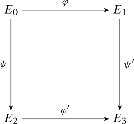
  The prover sends $E_2$ and $E_3$ to the verifier.

• 2. The verifier challenges the prover with a random bit ${\textsc {ch}}\leftarrow \{0,1\}$.

• 3. If ${\textsc {ch}}=0$, the prover reveals $P_2$ and $\varphi (P_2)$ (for example by sending the integers (a, b)).

  If ${\textsc {ch}}=1$, the prover reveals $\psi (P_1)$.

In both cases, the verifier accepts the proof if the points revealed have the right order and are the kernels of isogenies between the right curves. We iterate this process to reduce the cheating probability.

Note that the response to challenge 0 is two points while the response to challenge 1 is one point. In other words, at first sight, the responses have different lengths. Compression techniques can be used in this case to ensure that responses all have the same length (see Section 4.2 of [49]).

The following theorem is the main security result for this section. The basic ideas of the proof are by De Feo-Jao-Plût [19], but we give a slightly different formalisation that is required for our signature proof.

Theorem 6

If Problems 3 and 4 are computationally hard, then the interactive protocol defined above, repeated t times in parallel for a suitable parameter t, is a non-trivial canonical identification protocol that is secure against impersonation under passive attacks.

Proof

It is straightforward to check that the scheme is correct (in other words, the sigma protocol is complete). We now show that parallel executions of the sigma protocol are sound and honest verifier zero knowledge.

For soundness: Suppose $\mathcal {A}$ is an adversary that takes as input the public key and succeeds in the identification protocol with noticeable probability $\epsilon$. Given a challenge instance $(E_0,E_1,R_1,S_1, R_2, S_2, \varphi (R_2), \varphi (S_2))$ for Problem 3 we run $\mathcal {A}$ on this tuple as the public key. In the first round, $\mathcal {A}$ outputs commitments $(E_{i,2}, E_{i,3})$ for $1 \le i \le t$. We then send a challenge ${\textsc {ch}}\in \{ 0,1 \}^t$ to $\mathcal {A}$ and, with probability $\epsilon$ outputs a response ${\textsc {rsp}}$ that satisfies the verification algorithm. Now, we use the standard replay technique: Rewind $\mathcal {A}$ to the point where it had output its commitments and then respond with a different challenge ${\textsc {ch}}' \in \{ 0,1 \}^t$. With probability $\epsilon$, $\mathcal {A}$ outputs a valid response ${\textsc {rsp}}'$.

Now, choose some index i such that ${\textsc {ch}}_i \ne {\textsc {ch}}'_i$. We now restrict our focus to the components ${\textsc {cmt}}_i$, ${\textsc {rsp}}_i$ and ${\textsc {rsp}}_i'$. It means $\mathcal {A}$ sent $E_2, E_3$ and can answer both challenges ${\textsc {ch}}=0$ and ${\textsc {ch}}=1$ successfully. Hence we have an explicit description of the isogenies $\psi , \psi '$ and $\varphi '$ in the following diagram.

From this, one has an explicit description of an isogeny $\tilde{\varphi } = \hat{\psi '} \circ \varphi ' \circ \psi$ from $E_0$ to $E_1$. The degree of $\tilde{\varphi }$ is $\ell _1^{e_1} \ell _2^{2 e_2}$. One can determine $\ker ( \tilde{\varphi }) \cap E_0[ \ell _1^{e_1} ]$ by iteratively testing points in $E_0[ \ell _1^{j} ]$ for $j = 1, 2, \dots$. Hence, one determines the kernel of $\varphi$, as desired. This proves soundness.

Now we show honest verifier zero-knowledge. For this it suffices to show that one can simulate transcripts of the protocol without knowing the private key. When $b=0$ we simulate correctly by choosing $u,v \in \mathbb {Z}_{\ell _2^{e_2}}$ and setting $E_2 = E_0 / \langle u R_2 + v S_2 \rangle$ and $E_3 = E_1 / \langle u \varphi (R_2) + v \varphi ( S_2) \rangle$. When $b=1$ we choose a random curve $E_2$ and a random point $R \in E_2[ \ell _1^{e_1} ]$ and we publish $E_2, E_3 = E_2 / \langle R \rangle$ and answer with the point R (hence defining the isogeny). Although $(E_2, E_3 )$ are a priori not distributed correctly, the computational assumption of Problem 4 implies it is computationally hard to distinguish the simulation from the real game. Hence the scheme has computational zero knowledge.

Finally we prove the identification scheme is secure against impersonation under passive attacks. Let I be an impersonator for the scheme. Given a challenge instance $(E_0,E_1,R_1,S_1, R_2, S_2, \varphi (R_2), \varphi (S_2))$ for Problem 3 we run I on this tuple as the public key. We are required to provide I with a set of transcripts of honest executions of the scheme, but this is done using the simulation method used to show the sigma protocol has honest verifier zero knowledge. If I is able to succeed in its impersonation game then it breaks the soundness of the sigma protocol. We have already shown that if an adversary can break soundness then we can solve Problem 3. This completes the proof. $\square$

3.2 Classical Signature Scheme based on De Feo-Jao-Plût Identification Protocol

One can apply the Fiat-Shamir transform from Section 2.6 to the De Feo-Jao-Plût identification scheme to obtain a signature scheme. One can also check that the scheme is recoverable and so one can apply the Fiat-Shamir variant from Remark 1. In this section we fully specify the signature scheme resulting from the transform of Remark 1, together with some optimisations.

Our main focus is to minimise signature size. Hence, we use the most space-efficient variant of the Fiat-Shamir transform. Next we need to consider how to minimise the amount of data that needs to be sent to specify the isogenies. Several approaches were considered in Section 2.4. For the pair of vertical isogenies it seems to be most compact to represent them using a representation of the kernel (this is more efficient than specifying two paths in the isogeny graph), however this requires additional points in the public key. For the horizontal isogeny there are several possible approaches, but we think the most compact is to use the representation in terms of specifying roots of the modular polynomial. One can easily find other implementations that allow different tradeoffs of public key size versus signature size.

Key Generation Algorithm: On input a security parameter $\lambda$ generate a prime p with at least $4\lambda$ bits, such that $p=\ell _1^{e_1}\ell _2^{e_2}f\pm 1$, with $\ell _1,\ell _2,f$ small (ideally $f=1$, $\ell _1=2$, $\ell _2=3$) and $\ell _1^{e_1}\approx \ell _2^{e_2}$. Choose⁸ a supersingular elliptic curve $E_0$ with $\#E_0(\mathbb {F}_{p^2})=(\ell _1^{e_1}\ell _2^{e_2}f)^2$ and j-invariant $j_0$. Fix points $R_2, S_2 \in E_0( \mathbb {F}_{p^2} )[ \ell _2^{e_2} ]$ and a random primitive $\ell _1^{e_1}$-torsion point $P_1 \in E_0[ \ell _1^{e_1} ]$. Compute the isogeny $\varphi : E_0 \rightarrow E_1$ with kernel generated by $P_1$, and let $j_1$ be the j-invariant of the image curve. Set $R_2' = \varphi ( R_2 )$, $S_2' = \varphi (S_2)$. Choose a hash function H with $t = 2\lambda$ bits of output (see Remark 2). The secret key is $P_1$, and the public key is $(p,j_0,j_1,R_2, S_2, R_2', S_2', H)$. One can reduce the size of the public key by using different representations of isogeny paths, but for simplicity we use this variant.

Signature Algorithm: For $i=1,\ldots ,t$, choose random integers $0 \le \alpha _i < \ell _2^{e_2}$. Compute the isogeny $\psi _i : E_0 \rightarrow E_{2,i}$ with kernel generated by $R_{2} + [\alpha _i] S_{2}$ and let $j_{2,i} = j( E_{2,i} )$. Compute the isogeny $\psi _i' : E_1 \rightarrow E_{3,i}$ with kernel generated by $R_{2}' + [\alpha _i] S_{2}'$ and let $j_{3,i} = j( E_{3,i} )$. Compute $h=H(m,j_{2,1},\ldots ,j_{2,t},j_{3,1},\ldots ,j_{3,t})$ and parse the output as t challenge bits $b_i$. For $i=1,\ldots ,t$, if $b_i=0$ then set $z_i = \alpha _i$. If $b_i=1$ then compute $\psi _i(P_1)$ and compute a representation $z_i$ of the j-invariant $j_{2,i} \in \mathbb {F}_{p^2}$ and the isogeny with kernel generated by $\psi _i(P_1)$ (for example, as a sequence of integers representing which roots of the $\ell _1$-division polynomial to choose at each step of a non-backtracking walk, or using a compact representation of $\psi _i(P_1)$ in reference to a canonical basis of $E_{2,i}[ \ell _1^{e_1} ]$). Return the signature $\sigma =(h,z_1,\ldots ,z_{t})$.

Verification Algorithm: On input a message m, a signature $\sigma$ and a public key PK, recover the parameters $p,E_0,E_1$. For each $1 \le i \le t$, using the information provided by $z_i$, one recomputes the j-invariants $j_{2,i}, j_{3,i}$. In the case $b_i = 0$ this is done using $z_i = \alpha _i$ by computing the isogeny from $E_0$ with kernel generated by $R_2 + [\alpha _i] S_2$ and the isogeny from $E_1$ with generated by $R_2' + [\alpha _i] S_2'$. When $b_i = 1$ then the value $j_{2,i}$ is provided as part of $z_i$, together with a description of the isogeny from $E_{2,i}$ to $E_{3,i}$.

One then computes

$$\begin{aligned} h' = H( m, j_{2,1},\ldots ,j_{2,t},j_{3,1},\ldots ,j_{3,t}) \end{aligned}$$

and checks that the value equals h from the signature. The signature is accepted if this is true and is rejected otherwise.

Theorem 7

If Problems 3 and 4 are computationally hard then the first signature scheme is secure in the random oracle model under a chosen message attack.

Proof

This follows immediately from Theorem 4, Theorem 2 and Theorem 6. $\square$

Efficiency: As isogenies are of degree roughly $\sqrt{p}$, the scheme requires to use primes p of size $4\lambda$ to defeat meet-in-the-middle attacks. Assuming H is some fixed hash function and therefore not sent, the secret key is simply $x(P_1) \in \mathbb {F}_{p^2}$. A trivial representation requires $2\log p=8\lambda$ bits; however with a canonical ordering of the cyclic subgroups this can be reduced to $\frac{1}{2}\log p=2\lambda$ bits.

The public key is p and then $j_0, j_1, x(R_2), x(S_2), x(R_2'), x(S_2') \in \mathbb {F}_{p^2}$ which requires $13 \log _2(p) \approx 52 \lambda$ bits. The values of $j_0$, $x(R_2)$ and $x(S_2)$ can be canonically fixed by the protocol, in which case the public key is only $7\log p\approx 28\lambda$ bits. The values of $x(R_2')$ and $x(S_2')$ can also be avoided but at the expense of larger signature sizes. The signature size is analysed in Lemma 2.

De Feo et al [19] showed how to compute an $\ell ^e$-isogeny in around $e \log (e)$ exponentiations/Vélu computations using what they call an “optimal strategy”. Assuming quasi-linear cost ${\tilde{O}}(\log (p^2)) = {\tilde{O}}(\lambda )$ for the field operations, the total computational complexity of the signing and verifying algorithms is ${\tilde{O}}(\lambda ^3)$ bit operations.

Lemma 2

The average signature size of this scheme is

$$\begin{aligned} t \ + \ \tfrac{t}{2} \lceil \log _2( \ell _2^{e_2} )\rceil + \tfrac{t}{2} \left( 2 \lceil \log _2(p)\rceil + \lceil \log _2( \ell _1^{e_1} )\rceil \right) \approx 6 \lambda ^2 \end{aligned}$$

bits.

Proof

On average half the bits $b_i$ of the hash value are zero and half are one. When $b_i = 0$ we send an integer $\alpha _i$ such that $0 \le \alpha _i < \ell _2^{e_2}$, which requires $\lceil \log _2( \ell _2^{e_2} )\rceil \approx 2 \lambda$ bits. When $b_i = 1$ we need to send $j_{2,i} \in \mathbb {F}_{p^2}$, which requires $2 \lceil \log _2(p)\rceil$ bits, followed by a representation of the isogeny. One can represent a generator of the kernel of the isogeny with respect to some canonical generators $P_1', Q_1'$ of $E_{2,i}[ \ell _1^{e_1} ]$ as $\beta _i$ such that $0 \le \beta _i < \ell _1^{e_1}$, thus requiring $\lceil \log _2( \ell _1^{e_1} )\rceil$ bits. Alternatively one can represent the non-backtracking sequence of j-invariants in terms of an ordering on the roots of the $\ell _1$-th modular polynomial. This also can be done in $\lceil \log _2( \ell _1^{e_1} )\rceil$ bits. For security level $\lambda$ one can take $t = \lambda$ (as explained in Remark 2), giving $\ell _1^{e_1} \approx \ell _2^{e_2} \approx 2^{2\lambda }$, $p \approx 2^{4\lambda }$ and so signatures are around $6 \lambda ^2$ bits. The more conservative choice $t = 2 \lambda$ gives signatures of around $12 \lambda ^2$ bits. $\square$

3.3 Post-Quantum Signature Scheme based on De Feo-Jao-Plût Identification Protocol

Next, we describe the signature scheme resulting from applying Unruh’s transform to the identification scheme of De Feo-Jao-Plût, and we discuss its efficiency.

Key Generation Algorithm: On input a security parameter $\lambda$ generate a prime p with at least $6\lambda$ bits, such that $p=\ell _1^{e_1}\ell _2^{e_2}f\pm 1$, with $\ell _1,\ell _2,f$ small (ideally $f=1$, $\ell _1=2$, $\ell _2=3$) and $\ell _1^{e_1}\approx \ell _2^{e_2} > 2^{3 \lambda }$. Choose a supersingular elliptic curve $E_0$ with $\#E_0(\mathbb {F}_{p^2})=(\ell _1^{e_1}\ell _2^{e_2}f)^2$ and j-invariant $j_0$. Fix a canonical basis $\{R_2, S_2\}$ for $E_0( \mathbb {F}_{p^2} )[ \ell _2^{e_2} ]$ and a random primitive $\ell _1^{e_1}$-torsion point $P_1 \in E_0[ \ell _1^{e_1} ]$. Compute the isogeny $\varphi : E_0 \rightarrow E_1$ with kernel generated by $P_1$, and let $j_1$ be the j-invariant of the image curve. Set $R_2' = \varphi ( R_2 )$, $S_2' = \varphi (S_2)$. Choose a hash function $H:\{0,1\}^*\rightarrow \{0,1\}^t$ with $t = 3\lambda$ bits of output (see Remark 4), and two hash functions $G_i : \{ 0,1 \}^{N_i} \rightarrow \{ 0,1 \}^{N_i}$ for $i=0,1$, such that every element has polynomially many preimages. Here $N_i$ is an upper bound on the bitlength of the responses in the protocol when the challenge bit is i. The secret key is $P_1$, and the public key is $(p,j_0,j_1,R_2, S_2, R_2', S_2', H,G)$. One can reduce the size of the public key by using different representations of isogeny paths, but for simplicity we use this variant.

Signing Algorithm: For $i=1,\ldots ,t$, choose random integers $0 \le \alpha _i < \ell _2^{e_2}$. Compute the isogeny $\psi _i : E_0 \rightarrow E_{2,i}$ with kernel generated by $R_{2} + [\alpha _i] S_{2}$ and let $j_{2,i} = j( E_{2,i} )$. Compute the isogeny $\psi _i' : E_1 \rightarrow E_{3,i}$ with kernel generated by $R_{2}' + [\alpha _i] S_{2}'$ and let $j_{3,i} = j( E_{3,i} )$. For $i=1,\ldots ,t$, set $z_{i,0} = \alpha _i$ and $z_{i,1}$ as a representation of the j-invariant $j_{2,i} \in \mathbb {F}_{p^2}$ and the isogeny with kernel generated by $\psi _i(P_1)$ (for example, as a sequence of integers representing which roots of the $\ell _1$-modular polynomial to choose at each step of a non-backtracking walk, or using a compact representation of $\psi _i(P_1)$ in reference to a canonical basis of $E_{2,i}[ \ell _1^{e_1} ]$).

Compute $g_{i,0}=G_0(z_{i,0})$ and $g_{i,1}=G_1(z_{i,1})$ for $1\le i\le t$. Compute

$$\begin{aligned} h=H(m,j_{2,1},\ldots ,j_{2,t},j_{3,1},\ldots ,j_{3,t}, g_{1,0},g_{1,1},\dots ,g_{t,0},g_{t,1}) \end{aligned}$$

and parse the output as t challenge bits $h_i$. For $i=1,\ldots ,t$, set ${\textsc {rsp}}_i=z_{i,h_i}$. Return the signature

$$\begin{aligned} \sigma =(h,{\textsc {rsp}}_1,\ldots ,{\textsc {rsp}}_{t}, g_{1,1-h_1}, \dots , g_{t,1-h_t}). \end{aligned}$$

Verification Algorithm: On input a message m, a signature $\sigma$ and a public key PK, recover the parameters $p,E_0,E_1$. For each $1 \le i \le t$, using the information provided by ${\textsc {rsp}}_i$, one recomputes the j-invariants $j_{2,i}, j_{3,i}$. In the case $h_i = 0$ this is done using ${\textsc {rsp}}_i = \alpha _i$ by computing the isogeny from $E_0$ with kernel generated by $R_2 + [\alpha _i] S_2$ and the isogeny from $E_1$ with generated by $R_2' + [\alpha _i] S_2'$. When $h_i = 1$ then the value $j_{2,i}$ is provided as part of ${\textsc {rsp}}_i$, together with a description of the isogeny from $E_{2,i}$ to $E_{3,i}$.

The verifier computes $g_{i,h_i} = G_{h_i}( {\textsc {rsp}}_i )$ for $1 \le i \le t$ (padding to N bits using zeros) and checks that the hash value

$$\begin{aligned} h' = H(m,j_1, j_{2,1},\ldots ,j_{2,t}, g_{1,0}, g_{1,1}, \dots , g_{t,0}, g_{t,1}). \end{aligned}$$

is the same as h from the signature. In this case the verifier accepts the proof, otherwise it is rejected.

We now show that this scheme is a secure signature.

Theorem 8

If Problems 3 and 4 are computationally hard then the first signature scheme is secure in the quantum random oracle model under a chosen message attack.

Proof

This follows immediately from Theorem 5, Theorem 2 and Theorem 6. $\square$

Efficiency: There are four reasons why the post-quantum variant of the signature is less efficient than the variant in Section 3.2. First, the prime p is larger in the post-quantum case due to the quantum attack on the isogeny problem due to Biasse, Jao and Sankar [8]. Second, one must compute responses to both values of the challenge bit, which essentially doubles the computation compared with the non-post-quantum case. Thirdly, one needs to send the values $g_{i,j}$ as part of the signature, which increases signature size. Note that we have introduced an optimisation that only sends half the values $g_{i,j}$, since the missing values can be recomputed by the verifier. And fourth, the chosen value of t will be larger when aiming for quantum security, as per Remark 4.

We now compute the average signature size. When $h_i=0$, responses are of the form $\alpha _i$ for a random integer $0\le \alpha _i<\ell _2^{e_2}$, and thus requiring $N_0\approx \log {\ell _2}^{e_2}\approx \frac{1}{2}\log p$ bits each. When $h_i=1$, responses encode the j-invariant $j_{2,i}$, which takes $\lceil 2\log p\rceil$ bits to represent, and the isogeny with kernel generated by $\psi _i(P_1)$, which has degree $\ell _1^{e_1}$, and thus requires $\lceil \log \ell _1^{e_1}\rceil$ bits, for a total of $N_1\approx \frac{5}{2}\log p$. Finally, we note that the average response length $\frac{3}{2}\log p$ is doubled as in Unruh transform a commitment $g_{i,1-h_i}=G_{1-h_i}(z_{i,1-h_i})$ to the other challenge value is simultaneously transmitted. The average size of signatures is therefore $t+t\cdot 3\log p$. For $\lambda$ bits of security, we choose $\log p=6\lambda$ and $t=3\lambda$, obtaining an average signature size of $54\lambda ^2$.

4 Second Signature Scheme

We now present our main result. The main advantage of this scheme compared with the one in the previous section is that its security is based on the general problem of computing an isogeny between two supersingular curves, or equivalently on computing the endomorphism ring of a supersingular elliptic curve. Unlike the scheme in the previous section, the prime has no special property and no auxiliary points are revealed.

4.1 Identification Scheme Based on Endomorphism Ring Computation

The concept is similar to the graph isomorphism identification scheme, in which we reveal one of two graph isomorphisms, but never enough information to deduce the secret isomorphism.

As recalled in Section 2.4, although it is believed that computing endomorphism rings of supersingular elliptic curves is a hard computational problem in general, there are some particular curves for which it is easy.

The following construction is explained in Lemma 2 of [33]. We choose $E_0 : y^2 = x^3 + x$ over a field $\mathbb {F}_{p^2}$ where $p = 3\bmod {4}$ and $\#E_0( \mathbb {F}_{p^2} ) = (p+1)^2$. Unlike the scheme in Section 3, no constraint on the prime p or group order is necessary. We have $j(E_0) = 1728$. When $p=3\bmod 4$, the quaternion algebra $B_{p,\infty }$ ramified at p and $\infty$ can be canonically represented as $\mathbb {Q}\langle \mathbf{i},\mathbf{j}\rangle = \mathbb {Q}+ \mathbb {Q}\mathbf{i}+ \mathbb {Q}\mathbf{j}+ \mathbb {Q}\mathbf{k}$, where $\mathbf{i}^2=-1$, $\mathbf{j}^2=-p$ and $\mathbf{k}:=\mathbf{i}\mathbf{j}=-\mathbf{j}\mathbf{i}$. The endomorphism ring of $E_0$ is isomorphic to the maximal order ${\mathcal {O}}_0$ with $\mathbb {Z}$-basis $\{1,\mathbf{i},\frac{1+\mathbf{k}}{2},\frac{\mathbf{i}+\mathbf{j}}{2}\}$. Indeed, there is an isomorphism of quaternion algebras $\theta :B_{p,\infty }\rightarrow {{\,\mathrm{End}\,}}(E_0)\otimes \mathbb {Q}$ sending $(1,\mathbf{i},\mathbf{j},\mathbf{k})$ to $(1,\phi ,\pi ,\pi \phi )$ where $\pi (x,y) = (x^p,y^p)$ is the Frobenius endomorphism, and $\phi (x,y) = (-x,\iota y)$ with $\iota ^2=-1$.

Let L be the product of prime powers $\ell ^e$ up to $B = 2 \log (p)$ (this choice is based on Lemma 1). In other words, let $\ell _1, \dots , \ell _r$ be the list of all primes up to B and let $L = \prod _{i=1}^r \ell _i^{e_i}$ where $\ell _i^{e_i} \le B < \ell _i^{e_i + 1}$.

To generate the public and private keys, we take a random isogeny (walk in the graph) $\varphi : E_0\rightarrow E_1$ of powersmooth degree L and, using this knowledge, compute ${{\,\mathrm{End}\,}}(E_1)$. The public information is $E_1$. The secret is ${{\,\mathrm{End}\,}}(E_1)$, or equivalently a path from $E_0$ to $E_1$. Under the assumption that computing the endomorphism ring is hard, the secret key cannot be computed from the public key only.

To prove knowledge of $\varphi$ the prover will choose a random isogeny $\psi : E_1 \rightarrow E_2$ and give $E_2$ to the verifier. The verifier challenges the prover to give either the isogeny $\psi : E_1 \rightarrow E_2$ or an isogeny $\eta : E_0 \rightarrow E_2$. The fundamental problem is to find an isogeny $\eta$ that does not leak any information about $\varphi$ (in particular, the isogeny path corresponding to $\psi \circ \varphi$ would not be a secure response). Our scheme uses the following three algorithms, that are explained in detail in later sections, that allow a “pseudocanonical” isogeny $\eta$ to be computed (see Remark 5).

• Translate isogeny path to ideal: Given $E_0, \mathcal {O}_0= {{\,\mathrm{End}\,}}(E_0)$ and a chain of isogenies from $E_0$ to $E_1$, to compute $\mathcal {O}_1 = {{\,\mathrm{End}\,}}(E_1)$ and a left $\mathcal {O}_0$-ideal I whose right order is $\mathcal {O}_1$.

• Find new path: Given a left $\mathcal {O}_0$-ideal I corresponding to an isogeny $E_0 \rightarrow E_2$, to produce a new left $\mathcal {O}_0$-ideal J corresponding to an “independent” isogeny $E_0 \rightarrow E_2$ of powersmooth degree.

• Translate ideal to isogeny path: Given $E_0, \mathcal {O}_0, E_2, I$ such that I is a left $\mathcal {O}_0$-ideal whose right order is isomorphic to ${{\,\mathrm{End}\,}}(E_2)$, to compute a sequence of prime degree isogenies giving the path from $E_0$ to $E_2$.

Figure 1 gives the interaction between the prover and the verifier. One can see that Figure 1 gives a canonical, recoverable identification protocol, but it is not non-trivial as the challenge is only one bit. We repeat the protocol to reduce the cheating probability.

Fig. 1

New Identification Scheme

The isogenies involved in this protocol are summarized in the following diagram:

The two translation algorithms mentioned above in the $b=1$ case will be described in Section 4.4. They rely on the fact that ${{\,\mathrm{End}\,}}(E_0)$ is known. The algorithms are efficient when the degree of the random walk is powersmooth, and for this reason all isogenies in our protocols will be of powersmooth degree. The powersmooth version of the quaternion isogeny algorithm of Kohel-Lauter-Petit-Tignol will be described and analysed in Section 4.3. The random walks are taken of sufficiently large degree such that their output has close to uniform distribution, by Theorem 1 and Lemma 1.

In the next subsection we will prove the following result.

Theorem 9

Let $\lambda$ be a security parameter and $t \ge \lambda$. If Problem 6 is computationally hard, then the identification scheme obtained from t parallel executions of the protocol in Figure 1 is a non-trivial, recoverable canonical identification scheme that is secure against impersonation under (classical) passive attacks.

The advantage of this protocol over De Feo-Jao-Plût’s protocol is that it relies on a more standard and potentially harder computational problem. In the rest of this section we first give a proof of Theorem 9, then we provide details of the algorithms involved in our scheme.

4.2 Proof of Theorem 9

We shall prove that the sigma protocol in Figure 1 is complete, 2-special sound and honest verifier zero-knowledge. It follows that t parallel executions of the protocol is non-trivial. The theorem will then follow from Theorem 2 and Problem 6 (which implies that the relation being proved is a hard relation).

Note that a standard random-self-reduction [26] shows that the computational hardness of Problem 6 remains essentially the same if the curves are chosen according to a distribution that is close to uniform.

Completeness. Let $\varphi$ be an isogeny between $E_0$ and $E_1$ of B-powersmooth degree, for $B=O(\log p)$. If the challenge received is $b=0$, it is clear that the prover knows a valid isogeny $\psi : E_1\rightarrow E_2$, so the verifier accepts the proof. If $b=1$, the prover follows the procedure described above and the verifier accepts. In the next subsections we will show that this procedure is polynomial time.

2-special soundness. Let $(E_0, E_1)$ be an instance of Problem 6 and set it to be the public key for the scheme. Suppose we are given transcripts $( {\textsc {cmt}}, {\textsc {ch}}_1, {\textsc {ch}}_2, {\textsc {rsp}}_1, {\textsc {rsp}}_2 )$ for the single-bit scheme such that $\mathcal {V}( {\textsc {pk}}, {\textsc {cmt}}, {\textsc {ch}}_i , {\textsc {rsp}}_i ) = 1$ for all $i \in \{1, 2 \}$. Let $E_2 = {\textsc {cmt}}$. Since ${\textsc {ch}}_1 \ne {\textsc {ch}}_2$ the responses ${\textsc {rsp}}_1$ and ${\textsc {rsp}}_2$ therefore give two isogenies $\psi :E_1\rightarrow E_{2}$, $\eta :E_0\rightarrow E_{2}$. Given these two valid answers an extraction algorithm can compute an isogeny $\phi :E_0\rightarrow E_1$ as $\phi ={\hat{\psi }}\circ \eta$, where ${\hat{\psi }}$ is the dual isogeny of $\psi$. The extractor outputs $\phi$, which is a solution to Problem 6 (we stress that Problem 6 only asks for an arbitrary isogeny from $E_0$ to $E_1$). This is summarized in the following diagram.

Honest-verifier zero-knowledge. We shall prove that there exists a probabilistic polynomial time simulator $\mathcal {S}$ that outputs transcripts indistinguishable from transcripts of interactions with an honest verifier, in the sense that the two distributions are statistically close. Note that ${\mathcal {O}}_0 = {{\,\mathrm{End}\,}}( E_0 )$ is public information so is known to the simulator. The simulator starts by taking a random coin $b\leftarrow \{0,1\}$.

• If $b=0$, take a random walk from $E_1$ of powersmooth degree L, as in the real protocol, obtaining a curve $E_2$ and an isogeny $\psi :E_1\rightarrow E_2$. The simulator outputs the transcript $(E_2,0,\psi )$.

  

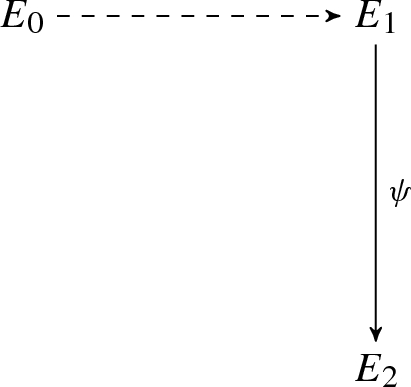
  In this case, it is clear that the distributions of every element in the transcript are the same as in the real interaction, as they are generated in the same way. This is possible because, when $b=0$, the secret is not required for the prover to answer the challenge.

• If $b=1$, take a random walk from $E_0$ of length L to obtain a curve $E_2$ and an isogeny $\mu :E_0\rightarrow E_2$, then proceed as in Step 4 of Figure 1 to produce another isogeny $\eta :E_0\rightarrow E_2$. The simulator outputs the transcript $(E_2,1,\eta )$.

The reason to output $\eta$ instead of $\mu$ is to ensure that the transcript distributions are indistinguishable from the distributions in the real scheme.

We first study the distribution of $E_2$ up to isomorphism. Let $X_r$ be the output of the random walk from $E_1$ to produce $j(E_2)$ in the real interaction, and let $X_s$ be the output of the random walk from $E_0$ to produce $j(E_2)$ in the simulation.

Let $\mathcal {G}$ be the set of all supersingular j-invariants, namely the vertex set of the isogeny graph. Note that $\#\mathcal {G}= N_p\approx p/12$. By Theorem 1 and Lemma 1, since the isogeny walks have degree L, we have, for any $j \in \mathcal {G}$

$$\begin{aligned} \left| \Pr (X_r= j )-\frac{1}{N_p}\right| \le \frac{1}{p^{1+\epsilon }},\left| \Pr (X_s= j )-\frac{1}{N_p}\right| \le \frac{1}{p^{1+\epsilon }}. \end{aligned}$$

Therefore

$$\begin{aligned} \begin{aligned} \sum _{j \in \mathcal {G}} \left| \Pr (X_r=j)-\Pr (X_s=j)\right|&\le N_p\cdot \max _i\left| \Pr (X_r=j)-\Pr (X_s=j)\right| \le \\&\le N_p\cdot \left( \frac{1}{p^{1+\epsilon }}+\frac{1}{p^{1+\epsilon }}\right) \approx \frac{1}{6p^{\epsilon }} \end{aligned} \end{aligned}$$

which is a negligible function of $\lambda$ for any constant $\epsilon >0$. In other words, the statistical distance, between the distribution of $j(E_2)$ in the real signing algorithm and the simulation, is negligible. Now, since $\eta$ is produced in the same way from $E_0$ and $E_2$ in the simulation and in the real protocol execution, we have that the statistical distance between the distributions of $\eta$ is also negligible. This follows from Lemma 3 in Section 4.3, which states that the output of the quaternion path algorithm does not depend on the input ideal, only on its ideal class.

4.3 Quaternion Isogeny Path Algorithm

In this section we sketch the quaternion isogeny algorithm from Kohel-Lauter-Petit-Tignol [33] and we evaluate its complexity when $p=3\bmod 4$. (The original paper does not give a precise complexity analysis; it only claims that the algorithm runs in heuristic probabilistic polynomial time.) This is the algorithm used for the Find new path procedure in the identification scheme.

The algorithm takes as input two maximal orders ${\mathcal {O}},{\mathcal {O}}'$ in the quaternion algebra $B_{p,\infty }$, and it returns a sequence of left ${\mathcal {O}}$-ideals $I_0={\mathcal {O}}\supset I_1\supset \ldots \supset I_e$ such that the right order of $I_e$ is in the same equivalence class as ${\mathcal {O}}'$. In addition, the output is such that the index of $I_{i+1}$ in $I_i$ is a small prime for all i. The paper [33] focuses on the case where the norm of $I_e$ is $\ell ^e$ for some integer e, but it mentions that the algorithm can be extended to the case of powersmooth norms. We will only describe and use the powersmooth version. In our application there are some efficiency advantages from using isogenies whose degree is a product of small powers of distinct primes, rather than a large power of a small prime.

Note that the ideals returned by the quaternion isogeny path algorithm (or equivalently the right orders of these ideals) correspond to vertices of the path in the quaternion algebra graph, and to a sequence of j-invariants by Deuring’s correspondence. In the next subsection we will describe how to make this correspondence explicit; here we focus on the quaternion algorithm itself.

An important feature of the algorithm is that paths between two arbitrary maximal orders ${\mathcal {O}}$ and ${\mathcal {O}}'$ are always constructed as a concatenation of two paths from each maximal order to a special maximal order. As mentioned above, in our protocol and the discussion below we fix ${\mathcal {O}}_0=\langle 1,\mathbf{i},\frac{1+\mathbf{k}}{2},\frac{\mathbf{i}+\mathbf{j}}{2}\rangle$ where $\mathbf{i}^2 = -1$ and $\mathbf{j}^2 = -p$. General references for maximal orders and ideals in quaternion algebras are [42, 43, 45].

We focus on the case where ${\mathcal {O}}={\mathcal {O}}_0$, and assume that instead of a second maximal order ${\mathcal {O}}'$ we are given the corresponding left ${\mathcal {O}}_0$-ideal I as input (the two variants of the problem are equivalent). This will be sufficient for our use of the algorithm. We assume that I is given by a $\mathbb {Z}$-basis of elements in ${\mathcal {O}}_0$. Note that in our context n(I) is known, as it is the degree of the known isogeny. Denote by $n( \alpha )$ and n(I) the norm of an element or ideal respectively. The equivalence class of maximal orders defines an equivalence class of ${\mathcal {O}}_0$-ideals, where two ideals I and J are in the same class if and only if $I=Jq$ with $q\in B_{p,\infty }^*$. Therefore our goal is, given a left ${\mathcal {O}}_0$-ideal I, to compute another left ${\mathcal {O}}_0$-ideal J with powersmooth norm in the same ideal class. Further, in order to be able to later apply Algorithm 2, we require the norm of I to be odd (but the Find new path algorithm also allows to find even norm ideals if desired). Without loss of generality we assume there is no integer $s>1$ such that $I\subset s{\mathcal {O}}_0$, and that $I\ne {\mathcal {O}}_0$. The algorithm proceeds as follows:

• 1. Compute an element $\delta \in I$ and an ideal $I' = I{\bar{\delta }}/n(I)$ of prime norm N.

• 2. Find $\beta \in I'$ with norm NS where S is powersmooth and odd.

• 3. Output $J = I'{\bar{\beta }}/N$.

Steps 1 and 3 of this algorithm rely on the following simple result [33, Lemma 5]: if I is a left $\mathcal {O}$-ideal of reduced norm N and $\alpha$ is an element of I, then $I{\bar{\alpha }}/N$ is a left $\mathcal {O}$-ideal of norm $n(\alpha )/N$. Clearly, I and J are in the same equivalence class.

To compute $\delta$ in Step 1, first a Minkowski-reduced basis $\{\alpha _1,\alpha _2,\alpha _3,\alpha _4\}$ of I is computed [35]. To obtain Lemma 3 below we make sure that the Minkowski basis is uniformly randomly chosen among all such bases⁹. Then random elements $\delta =\sum _ix_i\alpha _i$ are generated with integers $x_i$ in an interval $[-m,m]$, where m is determined later, until the norm of $\delta$ is equal to n(I) times a prime. A probable prime suffices in this context (actually Step 1 is not strictly needed but aims to simplify Step 2), so we can use the Miller-Rabin test to discard composite numbers with a large probability.

Step 2 is the core of the algorithm and actually consists of the following substeps:

• 2a. Find $\alpha$ such that $I'={\mathcal {O}}_0N+{\mathcal {O}}_0\alpha$.

• 2b. Find $\beta _1\in {\mathcal {O}}_0$ with odd norm $NS_1$, where $S_1$ is powersmooth.

• 2c. Find $\beta _2\in \mathbb {Z}\mathbf{j}+ \mathbb {Z}\mathbf{k}$ such that $\alpha =\beta _1\beta _2\bmod N{\mathcal {O}}_0$.

• 2d. Find $\beta _2' \in {\mathcal {O}}_0$ with odd powersmooth norm $S_2$ and $\lambda \in \mathbb {Z}_N^*$ such that $\beta _2'=\lambda \beta _2\bmod N{\mathcal {O}}_0$.

• 2e. Set $\beta =\beta _1\beta _2'$.

In Step 2a we need $\alpha \in I'$ such that $\gcd (n(\alpha ),N^2)=N$. This is easily achieved by taking $\alpha$ as a random small linear combination of a Minkowski basis, until the condition is met. Note that if $\alpha \in I'$ is such that $\gcd (n(\alpha ),N^2)=N$ then $J := {\mathcal {O}}_0 N + {\mathcal {O}}_0 \alpha \subseteq I'$ and $J \ne {\mathcal {O}}_0 N$. Since the norm of ${\mathcal {O}}_0 N$ is $N^2$ and N is prime it follows that the norm of J is N and so $J = I'$.

In Step 2b the algorithm actually searches for $\beta _1=a+b\mathbf{i}+c\mathbf{j}+d\mathbf{k}$. A large enough powersmooth number $S_1$ is fixed a priori, then the algorithm generates small random values of c, d until the norm equation $a^2+b^2=S_1-p(c^2+d^2)$ can be solved efficiently using Cornacchia’s algorithm (for example, until the right hand side is a prime equal to 1 modulo 4).

Step 2c is just linear algebra modulo N. As argued in [33] it has a negligible chance of failure, in which case one can just go back to Step 2b.

In Step 2d the algorithm a priori fixes $S_2$ large enough, then searches for integers $a,b,c,d,\lambda$ with $\lambda \notin N\mathbb {Z}$ such that $N^2(a^2+b^2)+p\left( (\lambda C+cN)^2+(\lambda D+dN)^2\right) =S_2$ where we have $\beta _2=C\mathbf{j}+D\mathbf{k}$. If necessary $S_2$ is multiplied by a small prime such that $p(C^2+D^2)S_2$ is a square modulo N, after which the equation is solved modulo N, leading to two solutions for $\lambda$. An arbitrary solution is chosen, and then looking at the equation modulo $N^2$ leads to a linear space of solutions for $(c,d)\in \mathbb {Z}_N$. The algorithm chooses random solutions until the equation

$$\begin{aligned} a^2+b^2=\left( S_2-p^2\left( (\lambda C+cN)^2+(\lambda D+dN)^2\right) \right) /N^2 \end{aligned}$$

can be efficiently solved with Cornacchia’s algorithm.

The overall algorithm is summarized in Algorithm 1. We now prove two lemmas on this algorithm. The first lemma shows that the output of this algorithm only depends on the ideal class of I but not on I itself. This is important in our identification protocol, as otherwise part of the secret isogeny $\varphi$ could potentially be recovered from $\eta$. The second lemma gives a precise complexity analysis of the algorithm, where [33] only showed probabilistic polynomial time complexity. Both lemmas are of independent interest.

Lemma 3

The output distribution of the quaternion isogeny path algorithm only depends on the equivalence class of its input. (In particular, the output distribution does not depend on the particular ideal class representative chosen for this input.)

Proof

Let $I_1$ and $I_2$ be two left ${\mathcal {O}}_0$-ideals in the same equivalence class, namely there exists $q\in B_{p,\infty }^*$ such that $I_2=I_1q$. We show that the distribution of the ideal $I'$ computed in Step 1 of the algorithm is identical for $I_1$ and $I_2$. As the inputs are not used anymore in the remainder of the algorithm this will prove the lemma.

In the first step the algorithm computes a Minkowski basis of its input, uniformly chosen among all possible Minkowski bases. Let $B_1=\{\alpha _{11},\alpha _{12},\alpha _{13},\alpha _{14}\}$ be a Minkowski basis of $I_1$. Then by multiplicativity of the norm we have that $B_2=\{\alpha _{11}q,$$\alpha _{12}q, \alpha _{13}q, \alpha _{14}q \}$ is a Minkowski basis of $I_2$. The algorithm then computes random elements $\delta =\sum _ix_i\alpha _i$ for integers $x_i$ in an interval $[-m,m]$. Clearly, for any element $\delta _1$ computed when the input is $I_1$, there corresponds an element $\delta _2=\delta _1q$ computed when the input is $I_2$. This is repeated until the norm of $\delta$ is a prime times n(I). As $n(I_2)=n(I_1)n(q)$ the stopping condition is equivalent for both. Finally, an ideal I of prime norm is computed as $I{\bar{\delta }}/n(I)$. Clearly when $\delta _2=\delta _1q$ we have $\frac{I_2{\bar{\delta }}_2}{n(I_2)}=\frac{I_1q{\bar{q}}{\bar{\delta }}_1}{n(q)n(I_1)}=\frac{I_1{\bar{\delta }}_1}{n(I_1)}$. This shows that the prime norm ideal computed in Step 1 only depends on the equivalence class of the input. $\square$

The expected running time given in the following lemma relies on several heuristics related to the factorization of numbers generated following certain distributions (see Section 2.8). Intuitively all these heuristics say that asymptotically those numbers behave in the same way as random numbers of the same size.

Lemma 4

Let $X:=\max \left| c_{ij}\right|$ where $c_{ij}\in \mathbb {Z}$ are integers such that $c_{i1}+c_{i2} \mathbf{i}+c_{i3}\frac{1+\mathbf{k}}{2}+c_{i4}\frac{\mathbf{i}+\mathbf{j}}{2}$ for $1 \le i \le 4$ forms a $\mathbb {Z}$-basis for I. If $\log X =O(\log p)$ then Algorithm 1 heuristically runs in time ${\tilde{O}}(\log ^3p)$, and produces an output of norm S with $\log (S)\approx \tfrac{7}{2} \log (p)$ which is $(\frac{7}{2} + o(1))\log p$-powersmooth.

Proof

The Minkowski basis can be computed in $O(\log ^2 X)$, for example using the algorithm of [35].

For generic ideals the reduced norms of all Minkowski basis elements¹⁰ are in $O(\sqrt{p})$ (see [33, Section 3.1]). In the first loop we initially set $m=\lceil \log p\rceil$. Assuming heuristically that the numbers N generated behave like random numbers we expect the box to produce some prime number. The resulting N will be in ${\tilde{O}}(\sqrt{p})$. For some non generic ideals the Minkowski basis may contain a pair of elements with norms significantly smaller than $O(\sqrt{p})$; in that case we can expect to finish the loop for smaller values of m by setting $x_3=x_4=0$, and to obtain some N of a smaller size.

Rabin’s pseudo-primality test performs a single modular exponentiation (modulo a number of size ${\tilde{O}}(\sqrt{p})$), and it is passed by composite numbers with a probability at most 1 / 4. The test can be repeated r times to decrease this probability to $1/4^r$. Assuming heuristically that the numbers tested behave like random numbers the test will only be repeated a significant amount of times on actual prime numbers, so in total it will be repeated $O(\log p)$ times. This leads to a total complexity of ${\tilde{O}}(\log ^3p)$ bit operations for the first loop using fast (quasi-linear) modular multiplication.

The other two loops involve solving equations of the form $x^2+y^2=M$. For such an equation to have solutions it is sufficient that M is a prime with $M=1\bmod 4$, a condition that is heuristically satisfied after $2\log M$ random trials. Choosing $S_1$ and $S_2$ as in the algorithm ensures that the right-hand term of the equation is positive, and (assuming this term behaves like a random number of the same size) is of the desired form for some choices (c, d), at least heuristically. Cornacchia’s algorithm runs in time ${\tilde{O}}(\log ^2 M)$, which is also ${\tilde{O}}(\log ^2 p)$ in the algorithm. The pseudo-primality tests will require ${\tilde{O}}(\log ^3p)$ operations in total, and their cost will dominate both loops.

Computing $\beta _2$ is just linear algebra modulo $N\approx {\tilde{O}}(\sqrt{p})$ and this cost can be neglected. The last two steps can similarly be neglected.

As a result, we get an overall cost of ${\tilde{O}}(\log ^3p)$ bit operations for the whole algorithm.

Let $s=\frac{7}{2}\log p$. We have $n(J)=n(I')n(\beta _1)n(\beta _2')/N^2$ so neglecting $\log \log$ factors $\log n(J)\approx \frac{1}{2}\log p+\log p+3\log p-\log p=\frac{7}{2}\log p$. We make the heuristic assumption that $\log n(J) = (\frac{7}{2} + o(1))\log p$. Moreover heuristically $\prod _{p_i^{e_i}<s} p_i^{e_i}\approx (s)^{s/\log s}\approx p^{7/2 + o(1)}$ so we can expect to find $S_1S_2$ that is s-powersmooth and of the correct size. $\square$

Remark 5

A subtle issue is to understand in what sense the output of Algorithm 1 is a “random” isogeny. The algorithm appears to make many random choices: first a “random ideal” $I'$ is chosen, then a “random” element $\beta _1$ is constructed, then an “arbitrary” $\beta _2$ is constructed, and finally the ideal J is output. However, a crucial observation is Lemma 3: since J is equivalent to I the output does not actually depend heavily on these choices (essentially the “choices all cancel each other out”). There is only a small set of actual isogenies $\eta$ that will be output by this algorithm (once the parameter L and other smoothness bounds are fixed). For this reason, we can view the output as “independent” of I (and hence of $\varphi$) and the isogeny $\eta$ as a “pseudo-canonical” choice of isogeny from $E_0$ to $E_2$.

4.4 Step-by-Step Deuring Correspondence

We now discuss algorithms to convert isogeny paths into paths in the quaternion algebra, and vice versa. This will be necessary in our protocols as we are sending curves and isogenies, whereas the process uses the quaternion isogeny algorithm.

All the isogeny paths that we will need to translate in our signature scheme will start from the special j-invariant $j_0=1728$. We recall (see beginning of Section 4.1) that this corresponds to the curve $E_0$ with equation $y^2=x^3+x$ and endomorphism ring ${{\,\mathrm{End}\,}}(E_0)=\langle 1,\phi , \frac{1+\pi \phi }{2},\frac{\pi + \phi }{2}\rangle$. Moreover there is an isomorphism of quaternion algebras sending $(1,\mathbf{i},\mathbf{j},\mathbf{k})$ to $(1,\phi ,\pi ,\pi \phi )$.

For any isogeny $\varphi :E_0\rightarrow E_1$ of degree n, we can associate a left ${{\,\mathrm{End}\,}}(E_0)$-ideal $I = \mathrm {Hom}(E_1,E_0) \varphi$ of norm n, corresponding to a left ${\mathcal {O}}_0$-ideal with the same norm in the quaternion algebra $B_{p,\infty }$. Conversely every left ${\mathcal {O}}_0$-ideal arises in this way [32, Section 5.3]. In our protocol we will need to make this correspondence explicit, namely we will need to pair up each isogeny from $E_0$ with the correct ${\mathcal {O}}_0$-ideal. Moreover we need to do this for “large” degree isogenies to ensure a good distribution via our random walk theorem.

4.4.1 Translating an ideal to an isogeny path.

Let $E_0$ and ${\mathcal {O}}_0 = {{\,\mathrm{End}\,}}(E_0)$ be given, together with a left ${\mathcal {O}}_0$-ideal I corresponding to an isogeny of degree n. We assume I is given as a $\mathbb {Z}$-basis $\{ \alpha _1, \dots , \alpha _4 \}$. The main idea to determine the corresponding isogeny explicitly is to determine its kernel [47].

Assume for the moment that n is a small prime. One can compute generators for all cyclic subgroups of $E_0[n]$, each one uniquely defining a degree n isogeny which can be computed with Vélu’s formulae. A generator P then corresponds to the basis $\{ \alpha _1, \dots , \alpha _4 \}$ if and only if $\alpha _j(P) = 0$ for all $1 \le j \le 4$. To evaluate $\alpha (P)$ with $\alpha \in I$ and $P\in E_0[n]$, we first write $\alpha =(u + v\mathbf{i}+ w\mathbf{j}+ x\mathbf{k})/2$, then we compute $P'$ such that $[2]P'=P$ and finally we evaluate $[u]P' + [v] \phi (P') + [w] \pi (P') + [x] \pi ( \phi (P'))$. To show that any such $P'$ works, write $\beta = u + v\mathbf{i}+ w\mathbf{j}+ x\mathbf{k}$. Since $\beta = \alpha \circ [2]$ it follows that $E_0[2] \subseteq \ker ( \beta )$. If $\beta (P') = 0$ then $\alpha (P) = \alpha ( [2]P' ) = (\alpha \circ [2] )(P') = \beta (P') = 0$. Since any other choice of $P'$ is $P' + T$ for some $T \in E_0[2]$ the choice of $P'$ does not matter.

An alternative to trying all subgroups is to choose a pair $\{ P_1, P_2 \}$ of generators for $E_0[n]$ and, for some $\alpha \in I$, solve the discrete logarithm instance (if possible) $\alpha (P_2) = [x] \alpha (P_1)$. It follows that $\alpha ( P_2 - [x] P_1 ) = 0$ and so we have determined a candidate point in the kernel of the isogeny. Both solutions are too expensive for large n.

When $n=\ell ^e$ the degree n isogeny can be decomposed into a composition of e degree $\ell$ isogenies. If P is a generator for the kernel of the degree $\ell ^e$ isogeny then $\ell ^{e-i+1}P$ is the kernel of the degree $\ell ^i$ isogeny corresponding to the first i steps. One can therefore perform the matching of ideals with kernels step-by-step with successive approximations of I or P respectively. This algorithm is more efficient than the previous one, but it still requires to compute $\ell ^e$ torsion points, which in general may be defined over a degree $\ell ^e$ extension of $\mathbb {F}_{p^2}$. To ensure that the $\ell ^e$ torsion is defined over $\mathbb {F}_{p^2}$ one can choose p such that $\ell ^e \mid (p \pm 1)$ as in the De Feo-Jao-Plût protocols; however for general p this translation algorithm will still be too expensive.

We solve this efficiency issue by using powersmooth degree isogenies in our protocols. When $n=\prod _i\ell _i^{e_i}$ with distinct primes $\ell _i$, one reduces to the prime power case as follows. For simplicity we assume that 2 does not divide n. The isogeny of degree n can be decomposed into a sequence of prime degree isogenies. For simplicity we assume the isogeny steps are always performed in increasing degree order; we can require that this is indeed the case in our protocols. However, rather than working with points on a sequence of elliptic curves, we work entirely on $E_0$. Using a Chinese Remainder Theorem-like representation, points in $E_0[n]$ can be represented as a sequence of points in $E_0[\ell _i^{e_i}]$. When one wishes to compute the corresponding sequence of isogenies $\varphi _{i} : E_{i-1} \rightarrow E_i$, each of degree $\ell _j^{e_j}$, it is necessary to transport the appropriate kernel points across to $E_{i-1}$ along the isogenies already computed.

Given a left ${\mathcal {O}}_0$-ideal I, Algorithm 2 progressively identifies the corresponding isogeny sequence. When determining points in $\ker ( \alpha ) \cap E_0[\ell _i^{e_i}]$ the algorithm uses a natural optimisation of reducing the coefficients of $\alpha$ modulo $\ell _i^{e_i}$.

In our protocols we will have $\ell _i^{e_i}=O(\log n)=O(\log p)$; moreover we will be using $O(\log p)$ different primes. The complexity of Algorithm 2 under these assumptions is given by the following lemma. Note that almost all primes $\ell _i$ are such that $\sqrt{B} < \ell _i \le B$ and so $e_i = 1$, hence we ignore the obvious $\ell$-adic speedups that can be obtained in the rare cases when $\ell _i$ is small.

Lemma 5

Let $n=\prod \ell _i^{e_i}$ with $\log n =O(\log p)$ and $\ell _i^{e_i}=O(\log p)$. Then Algorithm 2 can be implemented to run in time ${\tilde{O}}(\log ^6 p)$ bit operations for the first loop, and ${\tilde{O}}(\log ^5 p)$ for the rest of the algorithm.

Proof

Without any assumption on p the $\ell _i^{e_i}$ torsion points will generally be defined over $\ell _i^{e_i}$ degree extension fields, hence they will be of $O(\log ^2p)$ size. However the isogenies themselves will be rational, i.e. defined over $\mathbb {F}_{p^2}$. This means their kernel is defined by a polynomial over $\mathbb {F}_{p^2}$. Isogenies over $\mathbb {F}_{p^2}$ of degree d can be evaluated at any point in $\mathbb {F}_{p^2}$ using O(d) field operations in $\mathbb {F}_{p^2}$.

Let $d=\ell _i^{e_i}$. To compute a basis of the d-torsion, we first factor the division polynomial over $\mathbb {F}_{p^2}$. This polynomial has degree $O( d^2 ) = O( \log ^2 p )$. Using the algorithm in [30] this can be done in ${\tilde{O}}(\log ^4p)$ bit operations. Since the isogenies are defined over $\mathbb {F}_{p^2}$, this will give factors of degree at most $(d-1)/2$, each one corresponding to a cyclic subgroup. We then randomly choose some factor with a probability proportional to its degree, and we factor it over its splitting field, until we have found a basis of the d-torsion. After O(1) random choices we will have a basis of the d-torsion. Each factorization costs ${\tilde{O}}(\log ^5p)$ using the algorithm in [46], and verifying that two points generate the d-torsion can be done with O(d) field operations. It then takes O(d) field operations to compute generators for all kernels. As $r=O(\log p)$ we deduce that the first loop requires ${\tilde{O}}(\log ^6p)$ bit operations.

Computing $P_{ijk}$ involves Frobenius operations and multiplications by scalars bounded by d (and so $O(\log \log p)$ bits). This requires $O(\log \log p)$ field operations, that is a total of ${\tilde{O}}(\log ^3p)$ bit operations. Any cyclic subgroup of order $\ell _i^{e_i}$ is generated by a point $Q_i = aP_{i1}+bP_{i2}$, and the image of this point by $\alpha _{ik}$ is $aP_{i1k}+bP_{i2k}$. One can determine the integers a, b by an ECDLP computation or by testing random choices. There are roughly $\ell _i^{e_i}=O(\log p)$ subgroups, and testing each of them requires at most $O(\log \log p)$ field operations, so finding $Q_i$ requires ${\tilde{O}}(\log p)$ field operations. Evaluating $\varphi _{i-1}(Q_i)$ requires $O(\log ^2p)$ field operations. Computing the isogeny $\phi _i$ can be done in $O(\log p)$ field operations using Vélu’s formulae. As $r=O(\log p)$ we deduce that the second loop requires ${\tilde{O}}(\log ^5p)$ bit operations. $\square$

We stress that in our signature algorithm, Algorithm 2 will be run $O(\log p)$ times. However the torsion points are independent of both the messages and the keys, so they can be precomputed. Hence the “online” running time of Algorithm 2 is $\tilde{O}( \log ^5p)$ bit operations per execution.

4.4.2 Translating an isogeny path to an ideal.

Let $E_0, E_1, \dots , E_r$ be an isogeny path and suppose $\phi _{i} : E_{i-1} \rightarrow E_i$ is of degree $\ell _i^{e_i}$. We define $I_0={\mathcal {O}}_0$. Then for $i=1,\ldots ,r$ we compute an element $\alpha _i\in I_{i-1}$ and an ideal $I_i=I_{i-1}\ell _i^{e_i}+{\mathcal {O}}_0\alpha _i$ that corresponds to the isogeny $\phi _i\circ \cdots \circ \phi _1$. This is analogous in the power-smooth case to the notation $I_i$ as used in Section 4.3; in particular $I_0={\mathcal {O}}_0 \supset I_1\supset \ldots \supset I_r$. The idea is to determine suitable endomorphisms $\alpha _i \in I_{i-1}$ with the desired norm and that kill the required kernel point.

In our protocols we will have $\ell _i^{e_i}=O(\log n)=O(\log p)$; moreover we will be using $O(\log p)$ different primes. The complexity of Algorithm 3 for these parameters is given by the following lemma.

Lemma 6

Let $n=\prod _{i=1}^r \ell _i^{e_i}$ with $\log n=O(\log p)$ and $\ell _i^{e_i}=O(\log p)$. Assuming natural heuristics, Algorithm 3 can be implemented to run in expected time ${\tilde{O}}(\log ^4 p)$ and the output is a $\mathbb {Z}$-basis with integers bounded by X such that $\log X = O( \log p )$.

Proof

The input consists of a sequence of isogenies, and we remind that the representation of an isogeny is usually by explicitly specifying a kernel point (or else equivalent information, such as a polynomial whose roots are the kernel points). We remind that the $\ell _i^{e_i}$ torsion points will generally be defined over degree $\ell _i^{e_i}$ extension fields, hence they will be of $O(\log ^2p)$ size. Isogenies of degree d can be evaluated at any point using O(d) field operations.

When the degree is odd the isogeny $\phi _i$ is naturally given by a polynomial $\psi _i$ such that the roots of $\psi _i$ correspond to the x-coordinates of affine points in $\ker \varphi _i$. To identify a generator $Q_i$ we first factor $\psi _i$ over $\mathbb {F}_{p^2}$. Using the algorithm in [46] this can be done with ${\tilde{O}}(\log ^3p)$ bit operations. We choose a random irreducible factor with a probability proportional to its degree, we use this polynomial to define a field extension of $\mathbb {F}_{p^2}$, and we check whether the corresponding point is of order $\ell _i^{e_i}$. If not we choose another irreducible factor and we repeat. We expect to only need to repeat this O(1) times, and each step requires ${\tilde{O}}(\log p)$ bit operations. So the total cost for line 3 is ${\tilde{O}}(\log ^3p)$.

Step 4 requires $O(\log \log p)$ field operations to compute a point $Q_i'$ such that $[2]Q_i'=Q_i$. After that it mostly requires $O(\log p)$ field operations to compute the Frobenius map. The total cost of this step is therefore ${\tilde{O}}(\log ^3p)$.

Basis elements for all the ideals $I_i$ appearing in the algorithm can be reduced modulo ${\mathcal {O}}_0n$, hence their coefficients are of size $\log n=O(\log p)$.

To compute a random solution to $f_i$ modulo $\ell _i^{e_i}$, we choose uniformly random values for w, x, y, and when the resulting quadratic equation in z has solutions modulo $\ell _i^{e_i}$ we choose a random one. As $\ell _i^{e_i}=O(\log p)$ the cost of this step can be neglected. Computing $[\alpha _i](Q_i)$ requires $O(\log \log p)$ operations over a field of size $O(\log ^2p)$. On average we expect to repeat the loop $O(\ell _i^{e_i})=O(\log p)$ times, resulting in a total cost of ${\tilde{O}}(\log ^3p)$. Computing each $f_i$ costs ${\tilde{O}}(\log p)$ bit operations.

As $r=O(\log p)$ the total cost of the algorithm is ${\tilde{O}}(\log ^4p)$.

One can check that all integers in the algorithm are bounded in terms of n, and so coefficients are of size X where $\log X = O( \log n ) = O( \log p )$. $\square$

Recall that the condition $\log X = O( \log p )$ is needed in Lemma 4.

4.5 Classical Signature Scheme based on Endomorphism Ring Computation

In this section we give the details of our second signature scheme based on our new identification protocol, with security relying on computing the endomorphism ring of a supersingular elliptic curve.

Key Generation Algorithm: On input a security parameter $\lambda$ generate a prime p with $2\lambda$ bits, which is congruent to 3 modulo 4. Let $E_0 : y^2 = x^3 + Ax$ over $\mathbb {F}_p$ be supersingular, and let ${\mathcal {O}}_0 = {{\,\mathrm{End}\,}}( E_0 )$. Fix B, $S_1$, $S_2$ as small as possible¹¹ such that $S_{k}:=\prod _i\ell _{k,i}^{e_{k,i}}$, $\ell _{k,i}^{e_{k,i}}<B$, $\gcd (S_1,S_2)=1$, and $\prod \left( \frac{2\sqrt{\ell _{k,i}}}{\ell _{k,i}+1}\right) ^{e_{k,i}}<(p^{1+\epsilon })^{-1}$. Perform a random isogeny walk of degree $S_1$ from the curve $E_0$ with j-invariant $j_0=1728$ to a curve $E_1$ with j-invariant $j_1$. Compute $\mathcal {O}_1 = {{\,\mathrm{End}\,}}( E_1 )$ and the ideal I corresponding to this isogeny. Choose a hash function H with t bits of output (e.g., $t= \lambda$ or, more conservatively, $t = 2\lambda$). The public key is ${\textsc {pk}}= (p, j_1, H )$ and the secret key is ${\textsc {sk}}= \mathcal {O}_1$, or equivalently I.

Signing Algorithm: On input a message m and keys $({\textsc {pk}}, {\textsc {sk}})$, recover the parameters p and $j_1$. For $i=1,\ldots ,t$, generate a random isogeny walk $w_{i}$ of degree $S_2$, ending at a j-invariant $j_{2,i}$. Compute $h:=H(m,j_{2,1},\ldots ,j_{2,t})$ and parse the output as t challenge bits $b_i$. For $i=1,\ldots ,t$, if $b_i=1$ use $w_i$ and Algorithm 3 of Section 4.4 to compute the corresponding ideal $I_i$ and hence its right order ${\mathcal {O}}_{2,i} = {{\,\mathrm{End}\,}}( E_{2,i} )$, then use the algorithm of Section 4.3 on input $I I_i$ to compute a “fresh” path between ${\mathcal {O}}_0$ and ${\mathcal {O}}_{2,i}$, and finally use Algorithm 2 to compute an isogeny path $w_i'$ from $j_0$ to $j_{2,i}$. If $b_i=0$ set $z_i:=w_i$, otherwise set $z_i:=w_i'$. Return the signature $\sigma =(h,z_1,\ldots ,z_{t})$.

Verification Algorithm: On input a message m, a signature $\sigma$ and a public key ${\textsc {pk}}$, recover the parameters p and $j_1$. For each $1 \le i \le t$ one uses $z_i$ to compute the image curve $E_{2,i}$ of the isogeny. Hence the verifier recovers the j-invariants $j_{2,i}$ for $1 \le i \le t$. The verifier then recomputes the hash $H(m,j_{2,1},\ldots ,j_{2,t})$ and checks that the value is equal to h, accepting the signature if this is the case and rejecting otherwise.

We now show that this scheme is a secure signature.

Theorem 10

If Problem 6 is computationally hard then the signature scheme is secure in the random oracle model under a chosen message attack.

Proof

As shown in Section 4.2, if Problem 6 is computationally hard then the identification scheme (sigma protocol) has 2-special soundness and honest verifier zero-knowledge. Theorem 2 therefore implies that the identification scheme is secure against impersonation under passive attacks. It follows from Theorem 3 that the signature scheme is secure in the random oracle model. $\square$

Efficiency: As the best classical algorithm for computing the endomorphism ring of a supersingular elliptic curve runs in time $\tilde{O}(\sqrt{p})$ one can take $\log p=2\lambda$. By Theorem 1 and Lemma 1, taking $B\approx 2(1+\epsilon )\log p$ ensures that the outputs of random walks are distributed uniformly enough. Random walks then require $2(1+\epsilon )\log p$ bits to represent, so signatures are

$$\begin{aligned} t+\frac{t}{2}\left( 2(1+\epsilon )\lceil \log p\rceil +\frac{7}{2}\lceil \log p\rceil \right) \end{aligned}$$

bits on average, depending on the challenge bits. For $\lambda$ bits of security, we choose $t=\lambda$, so the average signature length is approximately $\lambda +(\frac{\lambda }{2})(4(1+\epsilon )\lambda +7\lambda )\approx \frac{1}{2}(11+4\epsilon )\lambda ^2\approx \frac{11}{2}\lambda ^2$. The conservative choice $t=2\lambda$ gives signatures of size approximately $11\lambda ^2$ bits.

Private keys are $2(1+\epsilon )\log p\approx 4\lambda$ bits if a canonical representation of the kernel of the isogeny between $E_0$ and $E_1$ is stored. This can be reduced to $2\lambda$ bits for generic $E_1$: if I is the ideal corresponding to this isogeny, it is sufficient to store another ideal J in the same class, and for generic $E_1$ there exists one ideal of norm $n\approx \sqrt{p}$. To represent this ideal in the most efficient way, it is sufficient to give n and a second integer defining the localization of I at every prime factor $\ell$ of n, for canonical embeddings of $B_{p,\infty }$ into $M_2(\mathbb {Q}_\ell )$, where $M_2(\mathbb {Q}_\ell )$ is the group of $2 \times 2$ matrices over the $\ell$-adics. This reduces storage costs to roughly $2\lambda$ bits. Public keys are $3\log p=6\lambda$ bits. A signature mostly requires t calls to the Algorithms of Sections 4.3 and 4.4 , for a total cost of ${\tilde{O}}(\lambda ^6)$. Verification requires to check $O(\lambda )$ isogeny walks, each one comprising $O(\lambda )$ steps with a cost $O(\lambda ^2)$ field operations each when modular polynomials are precomputed, hence a total cost of ${\tilde{O}}(\lambda ^6)$ bit operations (under the same heuristic assumptions as in Lemma 4).

Optimization with Non Backtracking Walks: In our description of the signature scheme we have allowed isogeny paths to “backtrack”. We made this choice to simplify the convergence analysis of random walks and because it does not affect the asymptotic complexity of our schemes significantly. However in practice at any concrete security parameter, it will be better to use non-backtracking random walks as they will converge more quickly to a uniform distribution [2].

4.6 Post-Quantum Signature Scheme based on Endomorphism Ring Computation

We briefly describe the signature scheme arising from applying Unruh’s transform to the identification protocol of Section 4.

Key Generation Algorithm: On input a security parameter $\lambda$ generate a prime p with $4\lambda$ bits, which is congruent to 3 modulo 4. Let $E_0 : y^2 = x^3 + Ax$ over $\mathbb {F}_p$ be supersingular, and let ${\mathcal {O}}_0 = {{\,\mathrm{End}\,}}( E_0 )$. Set $t= 3\lambda$. Fix B, $S_1$, $S_2$ as in the key generation algorithm of Section 4.5. Perform a random isogeny walk of degree $S_1$ from the curve $E_0$ with j-invariant $j_0=1728$ to a curve $E_1$ with j-invariant $j_1$. Compute $\mathcal {O}_1 = {{\,\mathrm{End}\,}}( E_1 )$ and the ideal I corresponding to this isogeny.

Choose a hash function $H : \{ 0,1 \}^* \rightarrow \{0,1\}^t$. Let $N_0 \approx 2\log p$ and $N_1 \approx \tfrac{7}{2} \log p$ be upper bounds for the bitlengths of the representations of isogeny paths in the algorithm, respectively in responses to challenges 0 and 1. For $i=0,1$ let $G_i : \{ 0,1 \}^{N_i} \rightarrow \{ 0,1 \}^{N_i}$ be a hash function such that every element has polynomially many preimages. The public key is ${\textsc {pk}}= (p, j_1, H, G_0,G_1 )$ and the secret key is ${\textsc {sk}}= \mathcal {O}_1$, or equivalently I.

Signing Algorithm: On input a message m and keys $({\textsc {pk}}, {\textsc {sk}})$, recover the parameters p and $j_1$. For $i=1,\ldots ,t$ generate a random isogeny walk $w_{i}$ of degree $S_2$, ending at a j-invariant $j_{2,i}$.

For $i=1,\ldots ,t$ apply Algorithm 3 of Section 4.4 to compute the ideal $I_i$ corresponding to the isogeny path $w_i$, then use the algorithm of Section 4.3 on input $I I_i$ to compute a “fresh” ideal corresponding to a path between ${\mathcal {O}}_0$ and ${\mathcal {O}}_{2,i}$, and finally use Algorithm 2 to compute an isogeny path $w_i'$ from $j_0$ to $j_{2,i}$.

Compute $g_{i,0} = G_0( w_i )$ and $g_{i,1} = G_1( w_i' )$ for $1 \le i \le t$, where the bitstrings $w_i$ and $w_i'$ are padded with zeroes to become binary strings of length N. Compute $h:=H(m,j_1,j_{2,1},\ldots ,j_{2,t}, g_{1,0}, g_{1,1}, \dots , g_{t,0}, g_{t,1} )$ and parse the output as t challenge bits $h_i$. For $i=1,\ldots ,t$, if $h_i=0$ then set ${\textsc {rsp}}_i = w_i$ and if $h_i = 1$ then set ${\textsc {rsp}}_i = w_i'$. Return the signature $\sigma =(h,{\textsc {rsp}}_1,\ldots ,{\textsc {rsp}}_{t}, g_{1,1-h_1}, \dots , g_{t, 1-h_t})$.

Verification Algorithm: On input a message m, a signature $\sigma$ and a public key ${\textsc {pk}}$, recover the parameters p and $j_1$.

For each $1 \le i \le t$ one uses ${\textsc {rsp}}_i$ to compute the image curve $E_{2,i}$ of the isogeny (if $h_i=0$ then ${\textsc {rsp}}_i$ is a path from $E_1$ and if $h_i = 1$ then it is a path from $E_0$). Hence the verifier recovers the j-invariants $j_{2,i}$ for $1 \le i \le t$.

The verifier then computes $g_{i,h_i} = G_{h_i}( {\textsc {rsp}}_i )$ for $1 \le i \le t$ (again padding to N bits using zeros). Finally the verifier computes the hash value

$$\begin{aligned} h' = H(m,j_1, j_{2,1},\ldots ,j_{2,t}, g_{1,0}, g_{1,1}, \dots , g_{t,0}, g_{t,1}). \end{aligned}$$

If $h' = h$ then the verifier accepts the signature and otherwise rejects.

We now show that this scheme is a secure signature.

Theorem 11

If Problem 6 is computationally hard then the signature scheme is secure in the quantum random oracle model under a chosen message attack.

Proof

As shown in Section 4.2, if Problem 6 is computationally hard then the identification scheme (sigma protocol) has 2-special soundness and honest verifier zero-knowledge. A result of Unruh [40] then implies that the signature scheme is secure in the quantum random oracle model. $\square$

Efficiency: For the same reasons as in the application of the Unruh transform to the De Feo-Jao-Plût scheme, this signature scheme is less efficient than its classical counterpart. Again, we only send half the values $g_{i,j}$, since the missing values can be recomputed by the verifier.

The average signature size is $t + t( (2\log p + \frac{7}{2}\log p) )$, on the basis that half the challenge bits are 0 and half of them are 1. For $\lambda$ bits of security, we choose $\log p = 4 \lambda$ and $t=3\lambda$. Then the average signature size is approximately $66 \lambda ^2$.

4.7 Comparison

Tables 1 and 2 summarize the main efficiency features of the four signature schemes based either on De Feo-Jao-Plût or on our new identification scheme, and on the Fiat-Shamir or Unruh transforms. The numbers provided were obtained by optimizing signature sizes first, then signing and verification time and finally key sizes; other trade-offs are of course possible. The scheme based on the De Feo-Jao-Plût identification protocol and Unruh transform was discovered independently in [49]; the version we give incorporates optimizations that reduce the signature sizes for the same security guarantees¹². Signatures based on De Feo-Jao-Plût identification protocol are simpler and somewhat more efficient than signatures based on our new identification protocol; however the latter have the advantage to rely on more standard and potentially harder computational problems. Schemes based on the Fiat-Shamir transform are more efficient than schemes based on Unruh’s transform; however the latter provide security guarantees against quantum adversaries.

Table 1 Asymptotic efficiency of four signature schemes using De Feo-Jao-Plût and our identification protocol, and Fiat-Shamir and Unruh transform, as a function of the security parameter $\lambda$. All sizes are in bits and computation costs are in bit operations

Table 2 Concrete efficiency of our signature schemes at security levels of 128 and 256 bits. Security level provided are against classical or quantum adversaries for schemes based on the Fiat-Shamir or Unruh transforms respectively. All sizes are in bits

Table 1 and a quick comparison with RSA signatures suggest that isogeny-based signatures schemes may be efficient enough for practical use. Indeed for RSA signatures, key sizes are cubic in the security parameter, and signing and verification times are respectively quasi-quadratic and quasi-linear in the key sizes (the latter assuming a small public key exponent is used), amounting to $\tilde{O}(\lambda ^3)$ and $\tilde{O}(\lambda ^6)$. As for concrete parameters, key sizes are much smaller for isogeny-based signatures than for RSA signatures and comparable to ECDSA signatures. Further work in this area should aim at decreasing signature sizes.

5 Conclusion

We have presented two signature schemes based on supersingular isogeny problems. Both schemes are built from a parallel execution of an identification scheme with bounded soundness, using the Fiat-Shamir transform. The first scheme is built directly from the De Feo-Jao-Plût identification protocol with some optimization. A similar scheme was given by Yoo, Azarderakhsh, Jalali, Jao and Soukharev [49]. The second scheme is more involved, and introduces a new randomisation method for isogeny paths. A crucial ingredient for our second protocol is the quaternion isogeny algorithm of Kohel-Lauter-Petit-Tignol [33] in the powersmooth case, for which we provide a more complete description and analysis. The first scheme is significantly more efficient, but the second one is based on an arguably more standard and potentially harder computational problem.

Our schemes rely on problems that can potentially resist quantum algorithms. However this family of problems are also are rather new in cryptography. Among all of them, we believe that the problem of computing the endomorphism ring of a supersingular elliptic curve (on which our second signature scheme relies) is the most natural one to consider from an algorithmic theory point of view, and it was the subject of Kohel’s PhD thesis in 1996 [32, Chapter 7]. The problem is also potentially harder than Problems 3 and 4 considered in previous works (and used in our first signature scheme). Yet, even that problem is far from having received the same scrutiny as more established cryptography problems like discrete logarithms or integer factoring. We hope that this paper will encourage the community to study its complexity.

References

M. Abdalla, J.H. An, M. Bellare, C. Namprempre, From identification to signatures via the Fiat–Shamir transform: minimizing assumptions for security and forward-security, in L.R. Knudsen, editor, EUROCRYPT 2002, volume 2332 of Lecture Notes in Computer Science (Springer, 2002), pp. 418–433
N. Alon, I. Benjamini, E. Lubetzky, S. Sodin, Non-backtracking random walks mix faster. Commun. Contem. Math. 9(4), 585–603 (2007)
R. Azarderakhsh, D. Jao, K. Kalach, B. Koziel, C. Leonardi, Key compression for isogeny-based cryptosystems, in AsiaPKC ’16 (ACM, New York, NY, USA, 2016), pp. 1–10
R. Beals, S. Brierley, O. Gray, A.W. Harrow, S. Kutin, N. Linden, D. Shepherd, M. Stather, Efficient distributed quantum computing. Proc. R. Soc. A 469(2153), 20120686 (2013)
M. Bellare, B. Poettering, D. Stebila, From identification to signatures, tightly: a framework and generic transforms, in J.H. Cheon, T. Takagi, editors, ASIACRYPT 2016, volume 10032 of Lecture Notes in Computer Science (Springer, 2016), pp. 435–464
D.J. Bernstein, Cost analysis of hash collisions: Will quantum computers make SHARCS obsolete?, in SHARCS’09 Special-purpose Hardware for Attacking Cryptographic Systems, p. 105 (2009)
G. Bertoni, J. Daemen, M. Peeters, G. Van Assche, Cryptographic sponge functions. Submission to NIST (Round 3) (2011)
J.-F. Biasse, D. Jao, A. Sankar, A quantum algorithm for computing isogenies between supersingular elliptic curves, in W. Meier, D. Mukhopadhyay, editors, INDOCRYPT 2014, volume 8885 of Lecture Notes in Computer Science (Springer, 2014), pp. 428–442
G. Bisson, A.V. Sutherland, Computing the endomorphism ring of an ordinary elliptic curve over a finite field. J. Number Theory 131(5), 815–831 (2011)
D.X. Charles, K.E. Lauter, E.Z. Goren, Cryptographic hash functions from expander graphs. J. Cryptol. 22(1), 93–113 (2009)
A.M. Childs, D. Jao, V. Soukharev, Constructing elliptic curve isogenies in quantum subexponential time. J. Math. Cryptol. 8(1), 1–29 (2014)
C. Costello, P. Longa, M. Naehrig, Efficient algorithms for supersingular isogeny Diffie–Hellman, in M. Robshaw, J. Katz, editors, CRYPTO 2016, volume 9814 of Lecture Notes in Computer Science (Springer, 2016), pp. 572–601
I. Damgård, On $\sigma $-protocols. Lecture Notes, University of Aarhus, Department for Computer Science (2010)
P. Deligne, La conjecture de Weil. I. Publications Mathématiques de l’Institut des Hautes Études Scientifiques 43(1), 273–307 (1974)
M. Deuring, Die Typen der Multiplikatorenringe elliptischer Funktionenkörper. Abhandlungen aus dem Mathematischen Seminar der Universität Hamburg 14, 197–272 (1941). https://doi.org/10.1007/BF02940746
L. Dewaghe, Isogénie entre courbes elliptiques. Util. Math. 55, 123–127 (1999)
K. Eisenträger, S. Hallgren, K.E. Lauter, T. Morrison, C. Petit, Supersingular isogeny graphs and endomorphism rings: reductions and solutions, in J.B. Nielsen, V. Rijmen, editors, Advances in Cryptology—EUROCRYPT 2018-37th Annual International Conference on the Theory and Applications of Cryptographic Techniques, Tel Aviv, Israel, April 29–May 3, 2018 Proceedings, Part III, volume 10822 of Lecture Notes in Computer Science (Springer, 2018), pp. 329–368
U. Feige, A. Fiat, A. Shamir, Zero-knowledge proofs of identity. J. Cryptol. 1(2), 77–94 (1988)
L. De Feo, D. Jao, J. Plût, Towards quantum-resistant cryptosystems from supersingular elliptic curve isogenies. J. Math. Cryptol. 8(3), 209–247 (2014)
A. Fiat, A. Shamir, How to prove yourself: practical solutions to identification and signature problems, in A.M. Odlyzko, editor, CRYPTO, volume 263 of Lecture Notes in Computer Science (Springer, 1986), pp. 186–194
S.D. Galbraith, Constructing isogenies between elliptic curves over finite fields. LMS J. Comput. Math. 2, 118–138 (1999)
S.D. Galbraith, C. Petit, B. Shani, Y. Bo Ti, On the security of supersingular isogeny cryptosystems, in J.H. Cheon, T. Takagi, editors, ASIACRYPT 2016, volume 10031 of Lecture Notes in Computer Science (Springer, 2016), pp. 63–91
S. Goldfeder, M. Chase, G. Zaverucha, Efficient post-quantum zero-knowledge and signatures (draft). Cryptology ePrint Archive, Report 2016/1110 (2016). http://eprint.iacr.org/2016/1110
S. Hoory, N. Linial, A. Wigderson, Expander graphs and their applications. Bull. Am. Math. Soc. 43, 439–561 (2006)
D. Jao, L. De Feo, Towards quantum-resistant cryptosystems from supersingular elliptic curve isogenies, in B.-Y. Yang, editor, PQCrypto 2011, volume 7071 of Lecture Notes in Computer Science (Springer, 2011), pp. 19–34
D. Jao, S.D. Miller, R. Venkatesan, Do all elliptic curves of the same order have the same difficulty of discrete log?, in B.K. Roy, editor, ASIACRYPT, volume 3788 of Lecture Notes in Computer Science (Springer, 2005), pp. 21–40
D. Jao, V. Soukharev, Isogeny-based quantum-resistant undeniable signatures, in M. Mosca, editor, PQCrypto 2014, volume 8772 of Lecture Notes in Computer Science (Springer, 2014), pp. 160–179
J. Katz, Digital Signatures. (Springer, Berlin, 2010)
J. Katz, Y. Lindell, Introduction to Modern Cryptography. (CRC Press, Boca Raton, 2014)
K.S. Kedlaya, C. Umans, Fast polynomial factorization and modular composition. SIAM J. Comput. 40(6), 1767–1802 (2011)
J. Kelsey, T. Kohno, Herding hash functions and the nostradamus attack, in S. Vaudenay, editor, EUROCRYPT 2006, volume 4004 of Lecture Notes in Computer Science (Springer, 2006), pp. 183–200
D. Kohel, Endomorphism rings of elliptic curves over finite fields. PhD thesis, University of California, Berkeley (1996)
D. Kohel, K. Lauter, C. Petit, J.-P. Tignol, On the quaternion $\ell $-isogeny path problem. LMS J. Comput. Math. 17A, 418–432 (2014)
G. Neven, N.P. Smart, B. Warinschi, Hash function requirements for schnorr signatures. J. Math. Cryptol. 3(1), 69–87 (2009)
P.Q. Nguyen, D. Stehlé, Low-dimensional lattice basis reduction revisited. ACM Trans. Algorithms 5(4) (2009)
C. Petit, Faster algorithms for isogeny problems using torsion point images, in T. Takagi, T. Peyrin, editors, Advances in Cryptology—ASIACRYPT 2017-23rd International Conference on the Theory and Applications of Cryptology and Information Security, Hong Kong, China, December 3–7, 2017, Proceedings, Part II, volume 10625 of Lecture Notes in Computer Science (Springer, 2017), pp. 330–353
C. Petit, K.E. Lauter, Hard and easy problems for supersingular isogeny graphs. IACR Cryptology ePrint Archive 2017, 962 (2017)
A.K. Pizer, Ramanujan graphs and Hecke operators. Bull. Am. Math. Soc. 23(1), 127–137 (1990)
J.H. Silverman, The Arithmetic of Elliptic Curves. (Springer, Berlin, 1986)
D. Unruh, Non-interactive zero-knowledge proofs in the quantum random oracle model, in E. Oswald, M. Fischlin, editors, EUROCRYPT 2015, volume 9057 of Lecture Notes in Computer Science (Springer, 2015), pp. 755–784
D. Venturi, Zero-knowledge proofs and applications. Lecture Notes, University of Rome (2015)
M.-F. Vignéras, The arithmetic of quaternion algebra (2006). http://maths.nju.edu.cn/~guoxj/notes/qa.pdf
M.-F. Vignéras, Arithmétique des algébres de quaternions. (Springer, Berlin, 1980)
J. Vélu, Isogénies entre courbes elliptiques. Communications de l’Académie royale des Sciences de Paris 273, 238–241 (1971)
J. Voight, Quaternion algebras (2017). https://math.dartmouth.edu/~jvoight/quat-book.pdf
J. von zur Gathen, V. Shoup, Computing Frobenius maps and factoring polynomials. Comput. Complex. 2, 187–224 (1992)
W.C. Waterhouse, Abelian varieties over finite fields. Annales scientifiques de l’E.N.S. 2, 521–560 (1969)
S. Xi, H. Tian, Y. Wang, Toward quantum-resistant strong designated verifier signature from isogenies. Int. J. Grid Util. Comput. 5(2), 292–296 (2012)
Y. Yoo, R. Azarderakhsh, A. Jalali, D. Jao, V. Soukharev, A post-quantum digital signature scheme based on supersingular isogenies, in Financial Crypto, vol. 2017 (2017)
Acknowledgements
We thank Dominique Unruh for his patient explanations of his transform and related issues. We also thank David Pointcheval and Ali El Kaafarani for discussions related to this paper, and all anonymous reviewers of this paper for their comments. Research from the second author was supported by a research grant from the UK government. The third author was supported by a PhD formation grant from the Spanish government, co-financed by the ESF (Ayudas para contratos predoctorales para la formación de doctores 2016).
Author information
Authors and Affiliations
Corresponding author
Additional information
Communicated by Kenneth G. Paterson.
Publisher's Note
Springer Nature remains neutral with regard to jurisdictional claims in published maps and institutional affiliations.
Rights and permissions
OpenAccess This article is distributed under the terms of the Creative Commons Attribution 4.0 International License (http://creativecommons.org/licenses/by/4.0/), which permits unrestricted use, distribution, and reproduction in any medium, provided you give appropriate credit to the original author(s) and the source, provide a link to the Creative Commons license, and indicate if changes were made.
About this article
Cite this article
Galbraith, S.D., Petit, C. & Silva, J. Identification Protocols and Signature Schemes Based on Supersingular Isogeny Problems. J Cryptol 33, 130–175 (2020). https://doi.org/10.1007/s00145-019-09316-0
Received:
Revised:
Published:
Issue Date:
DOI: https://doi.org/10.1007/s00145-019-09316-0