A Theory for the Composition of Concurrent Processes

Abstract

In this paper, we provide a theory for the operators composing concurrent processes. Open pNets (parameterised networks of synchronised automata) are new semantic objects that we propose for defining the semantics of composition operators. This paper defines the operational semantics of open pNets, using “open transitions” that include symbolic hypotheses on the behaviour of the pNets “holes”. We discuss when this semantics can be finite and how to compute it symbolically, and we illustrate this construction on a simple operator. This paper also defines a bisimulation equivalence between open pNets, and shows its decidability together with a congruence theorem.

This work was partially funded by the Associated Team FM4CPS between INRIA and ECNU, Shanghai.

These keywords were added by machine and not by the authors. This process is experimental and the keywords may be updated as the learning algorithm improves.

1 Introduction

In the nineties, several works extended the basic behavioural models based on labelled transition systems to address value-passing or parameterised systems, using various symbolic encodings of the transitions [1–4]. In [4], Lin addressed value-passing calculi, for which he developed a symbolic behavioural semantics, and proved algebraic properties. Separately Rathke [5] defined another symbolic semantics for a parameterised broadcast calculus, together with strong and weak bisimulation equivalences, and developed a symbolic model-checker based on a tableau method for these processes. 30 years later, no practical verification approach and no verification platform are using this kind of approaches to provide proof methods for value-passing processes or open process expressions. This article proposes a new approach to study concurrent and distributed systems based on a semantic formalism featuring: (1) low-level description of behaviours (transition systems) with explicit data parameters, and hierarchical structure, (2) flexible composition and synchronisation mechanism, (3) finite representation of the behavioural semantics using symbolic representations of sets of behaviours.

Parameterised Networks of synchronised automata (pNets) was proposed to give a behavioural specification formalism for distributed systems. It inherited from the work of Arnold on synchronisation vectors [6]. In previous work [7], we showed that pNets can be used to represent the behavioural semantics of a system including value-passing and many kinds of synchronisation methods. We used these results to give the semantics of various constructs and languages for distributed objects, and to build a platform for design and verification of distributed software components [8, 9]. The parameterised and hierarchical nature of pNets allows for compact models easy to generate from applications in high-level languages. Their structure is static, but unbounded, and this allows for model-checking approaches even for reconfigurable applications. Closed pNets were used to encode fully defined programs or systems, while open pNets have “holes”, playing the role of process parameters. Such open systems can be used to define composition operators. The challenge raised by the research on open pNets is due to its “open” nature and to the existence of holes and parameters.

Contribution. The aim of this paper is to provide a theory for the operators composing concurrent processes. This theory is based on the definition of operators as open pNets. By defining the operational semantics of open pNets, using open transitions that include symbolic hypotheses on the behaviour of the pNets holes, we can define a strong bisimulation equivalence between open pNets, and show its decidability. This work highlights the possibility to automatically infer proof obligations, in the form of predicate inclusion, that have to be verified to prove the equivalence of operators. These results allow us to envision the semi-automatic proof of equivalence between operators for composing processes.

Related Works. A number of fundamental works have been published on symbolic or open bisimulations, with varying vocabulary. In this section, we only list works that are directly related to our approach.

The closest research (and oldest) is from De Simone [1], who defines Specification Rules and a FH-bisimulation equivalence, that were one of our main inspiration for the open-transition concept. Some years later, Rensink [10] defines a generic notion of conditional transition systems and studies relations between FH-bisimulation and others. We believe that in the work of De Simone context and in ours, the relations coincide, and that Rensink work differs mainly in presence of recursive binding constructs that we do not consider.

In [3, 4] Hennessy and Lin developed the theory of symbolic transition graphs (STG), and the associated symbolic (early and late) bisimulations, they also study STGs with assignments which can be a model for message-passing processes. These are clearly related to our parameterised LTSs, though they are more specifically addressing the action algebra of value-passing CCS expressions. [3] also gives an algorithm for computing symbolic bisimulation, but only for symbolic finite trees. An interesting variant was developped by Hennessy and Rathke [5], concerning a calculus of broadcasting systems (CBS) and a symbolic bisimulation. The main characteristic of this calculus is that communication is “one-to-many”, and non blocking, so the definitions of semantics and equivalences differ significantly from previous works. Later, J. Rathke proposed a model-checker for CBS based on a sound tableau method over symbolic graphs. Another important similarity between the works on STGs, CBS, and ours is the use of an auxiliary proof system on value expressions. Remark that pNets can encode both value-passing CCS and CBS, but also other communication and synchronisation schemas.

More recently, Deng [11] gave an open bisimulation for $\pi$-calculus based on STG, which used a predicate equation system whose greatest solution characterizes the condition under which the two STGs are bisimilar. There is here a potential relation with our work: if the number of states and branching of the symbolic model is finite, then their algorithm can terminate; a similar approach may help us to compute our FH-bisimulation.

Finally, there are numerous works on subclasses of infinite-state programs or parameterised systems, seeking decidability properties, and sometimes model-checking or equivalence checking algorithms. For example [12] proposed a model checker to verify the safety and liveness properties on infinite-state programs. They symbolically encode transitions and states using predicates, including affine constraints on integer variables. Another very different approach is used by [13], relying on a dedicated model based on network grammars and regular languages.

Structure. Section 2 extends the previous definition of pNets [7] to fit the needs of the open pNets. Section 3 gives their operational semantics based on open transitions, and proves that this semantics is finite under reasonable conditions. In Sect. 4 we introduce an equivalence called FH-bisimulation, and prove its decidability. All sections are illustrated by a running example encoding a Lotos operator. Section 5 proves a crucial composition theorem. Finally Sect. 6 concludes and discusses future work.

2 Parameterised Networks (pNets): Definition

This section introduces pNets and the notations we will use in this paper. Then it gives the formal definition of pNet structures, together with an operational semantics for open pNets.

pNets are tree-like structures, where the leaves are either parameterised labelled transition systems (pLTSs), expressing the behaviour of basic processes, or holes, used as placeholders for unknown processes, of which we only specify the set of possible actions, this set is named the sort. Nodes of the tree (pNet nodes) are synchronising artifacts, using a set of synchronisation vectors that express the possible synchronisation between the parameterised actions of a subset of the sub-trees.

Notations. We extensively use indexed structures over some countable indexed sets, which are equivalent to mappings over the countable set. $a_i^{i\in I}$ denotes a family of elements $a_i$ indexed over the set I. $a_i^{i\in I}$ defines both I the set over which the family is indexed (called range), and $a_i$ the elements of the family. E.g., $a^{i\in \{3\}}$ is the mapping with a single entry a at index 3 ; abbreviated in the following. When this is not ambiguous, we shall use notations for sets, and typically write “indexed set over I” when formally we should speak of multisets, and write $x\in a_i^{i\in I}$ to mean $\exists i\in I.\, x=a_i$. An empty family is denoted $\emptyset$. We denote classically $\overline{a}$ a family when the indexing set is not meaningful. $\uplus$ is the disjoint union on indexed sets.

Term Algebra. Our models rely on a notion of parameterised actions, that are symbolic expressions using data types and variables. As our model aims at encoding the low-level behaviour of possibly very different programming languages, we do not want to impose one specific algebra for denoting actions, nor any specific communication mechanism. So we leave unspecified the constructors of the algebra that will allow building expressions and actions. Moreover, we use a generic action interaction mechanism, based on (some sort of) unification between two or more action expressions, to express various kinds of communication or synchronisation mechanisms.

Formally, we assume the existence of a term algebra $\mathcal {T}_{\varSigma ,\mathcal P}$, where $\varSigma$ is the signature of the data and action constructors, and $\mathcal P$ a set of variables. Within $\mathcal {T}_{\varSigma ,\mathcal P}$, we distinguish a set of data expressions $\mathcal {E}_\mathcal P$, including a set of boolean expressions $\mathcal {B}_{\mathcal P}$ ($\mathcal {B}_{\mathcal P}\subseteq \mathcal {E}_\mathcal P$). On top of $\mathcal {E}_\mathcal P$ we build the action algebra $\mathcal {A}_\mathcal P$, with $\mathcal {A}_P\subseteq \mathcal {T}_\mathcal P, \mathcal {E}_P\cap \mathcal {A}_P=\emptyset$; naturally action terms will use data expressions as subterms. To be able to reason about the data flow between pLTSs, we distinguish input variables of the form ?x within terms; the function vars(t) identifies the set of variables in a term $t\in \mathcal {T}$, and iv(t) returns its input variables.

pNets can encode naturally the notion of input actions in value-passing CCS [14] or of usual point-to-point message passing calculi, but it also allows for more general mechanisms, like gate negociation in Lotos, or broadcast communications. Using our notations, value-passing actions à la CCS would be encoded as $a(?x_1,...,?x_n)$ for inputs, $a(v_1,..,v_n)$ for outputs (in which $v_i$ are action terms containing no input variables). We can also use more complex action structure such as Meije-SCCS action monoids, like in a.b, $a^{f(n)}$ (see [1]). The expressiveness of the synchronisation constructs will depend on the action algebra.

2.1 The (open) pNets Core Model

A pLTS is a labelled transition system with variables; variables can be manipulated, defined, or accessed inside states, actions, guards, and assignments. Without loss of generality and to simplify the formalisation, we suppose here that variables are local to each state: each state has its set of variables disjoint from the others. Transmitting variable values from one state to the other can be done by explicit assignment. Note that we make no assumption on finiteness of the set of states nor on finite branching of the transition relation.

We first define the set of actions a pLTS can use, let a range over action labels, $\textit{op}$ are operators, and $x_i$ range over variable names. Action terms are:

The input variables in an action term are those marked with a . We additionally suppose that each input variable does not appear somewhere else in the same action term: $p_i=?x\Rightarrow \forall j\ne i.\, x\notin vars(p_j)$

Definition 1

(pLTS). A pLTS is a tuple $pLTS\triangleq \langle \langle S,s_0, \rightarrow \rangle \rangle$ where:

• S is a set of states.

• $s_0 \in S$ is the initial state.

• $\rightarrow \subseteq S \times L \times S$ is the transition relation and L is the set of labels of the form $\langle \alpha ,~e_b,~(x_j\!:= {e}_j)^{j\in J}\rangle$, where $\alpha \in \mathcal {A}$ is a parameterised action, $e_b \in \mathcal {B}$ is a guard, and the variables $x_j\in P$ are assigned the expressions $e_j\in \mathcal {E}$. If $s \xrightarrow {\langle \alpha ,~e_b,~(x_j\!:= {e}_j)^{j\in J}\rangle } s'\in \rightarrow$ then ${ iv}(\alpha )\!\subseteq \! vars(s')$, $vars(\alpha )\backslash { iv}(\alpha )\!\subseteq \! vars(s)$, $vars(e_b)\!\subseteq \! vars(s')$, and $\forall j\!\in \! J .\,vars(e_j)\!\subseteq \! vars(s)\wedge x_j\!\in \!vars(s')$.

Now we define pNet nodes, as constructors for hierarchical behavioural structures. A pNet has a set of sub-pNets that can be either pNets or pLTSs, and a set of Holes, playing the role of process parameters.

A composite pNet consists of a set of sub-pNets exposing a set of actions, each of them triggering internal actions in each of the sub-pNets. The synchronisation between global actions and internal actions is given by synchronisation vectors: a synchronisation vector synchronises one or several internal actions, and exposes a single resulting global action. Actions involved at the pNet level (in the synchronisation vectors) do not need to distinguish between input and output variables. Action terms for pNets are defined as follows:

Definition 2

(pNets). A pNet is a hierarchical structure where leaves are pLTSs and holes:

${ pNet}\triangleq pLTS~|~\langle \langle { pNet}_i^{i\in I}, S_j^{j\in J}, { SV}_k^{k\in K}\rangle \rangle$ where

• $I \in \mathcal {I}$ is the set over which sub-pNets are indexed.

• ${ pNet}_i^{i\in I}$ is the family of sub-pNets.

• $J\in \mathcal {I}_\mathcal P$ is the set over which holes are indexed. I and J are disjoint: $I\cap J=\emptyset$, $I\cup J\ne \emptyset$

• $S_j \subseteq \mathcal {A}_S$ is a set of action terms, denoting the ${{\mathrm{Sort}}}$ of hole j.

• ${ SV}_k^{k\in K}$ is a set of synchronisation vectors ($K\in \mathcal {I}_\mathcal P$). $\forall k\!\in \! K, { SV}_k\!=\!\alpha _{l}^{l\in I_k \uplus J_k}\rightarrow \alpha '_k$ where $\alpha '_k\in \mathcal {A}_\mathcal P$, $I_k\subseteq I$, $J_k\subseteq J$, $\forall i\!\in \! I_k.\,\alpha _{i}\!\in \!{{\mathrm{Sort}}}({ pNet}_i)$, $\forall j\!\in \! J_k.\,\alpha _{j}\!\in \!S_j$, and $vars(\alpha '_k)\subseteq \bigcup _{l\in I_k\uplus J_k}{vars({\alpha _l})}$. The global action of a vector ${ SV}_k$ is ${{\mathrm{Label}}}({ SV}_k) = \alpha '_k$.

Fig. 1.

Two pNet encodings for Enable

The preceding definition relies on the auxiliary functions below:

Definition 3

(Sorts, Holes, Leaves of pNets).

• The sort of a pNet is its signature, i.e. the set of actions it can perform. In the definition of sorts, we do not need to distinguish input variables (that specify the dataflow within LTSs), so for computing LTS sorts, we use a substitution operator¹ to remove the input marker of variables. Formally:

  $$\begin{aligned} \begin{array}{l} {{\mathrm{Sort}}}(\langle \langle S,s_0, \rightarrow \rangle \rangle ) = \{\alpha \{\{\!x \leftarrow ?x| x\in { iv}(\alpha )\!\}\}|s \xrightarrow {\langle \alpha ,~e_b,~(x_j\!:= {e}_j)^{j\in J}\rangle } s'\in \rightarrow \} \\ {{\mathrm{Sort}}}(\langle \langle \overline{{ pNet}}, \overline{{ S}}, \overline{{ SV}}\rangle \rangle ) =\{\alpha '_k |\, \alpha _j^{j\in J_k}\rightarrow \alpha '_k\in \overline{{ SV}}\} \end{array} \end{aligned}$$

• The set of holes of a pNet is defined inductively; the sets of holes in a pNet node and its subnets are all disjoint:

  $$\begin{aligned} \begin{array}{l} {{\mathrm{Holes}}}(\langle \langle S,s_0, \rightarrow \rangle \rangle ) \!=\! \emptyset \\ {{\mathrm{Holes}}}(\langle \langle { pNet}_i^{i\in I}\!,S_j^{j\in J}\!, \overline{{SV}}\rangle \rangle ) =J\cup {\displaystyle \bigcup _{i\in I}{{\mathrm{Holes}}}({ pNet}_i)}\\ \forall i\in I.\, {{\mathrm{Holes}}}({ pNet}_i)\cap J=\emptyset \\ \forall i_1,i_2\in I.\,i_1\ne i_2\Rightarrow {{\mathrm{Holes}}}({ pNet}_{i_1})\cap {{\mathrm{Holes}}}({ pNet}_{i_2})=\emptyset \end{array} \end{aligned}$$

• The set of leaves of a pNet is the set of all pLTSs occurring in the structure, defined inductively as:

  $$\begin{aligned} \begin{array}{l} {{\mathrm{Leaves}}}(\langle \langle S,s_0, \rightarrow \rangle \rangle ) \!=\! \{ \langle \langle S,s_0, \rightarrow \rangle \rangle \}\\ {{\mathrm{Leaves}}}(\langle \langle { pNet}_i^{i\in I}\!,S_j^{j\in J}\!, \overline{{ SV}}\rangle \rangle ) = {\displaystyle \bigcup _{i\in I}{{\mathrm{Leaves}}}({ pNet}_i)} \end{array} \end{aligned}$$

A pNet Q is closed if it has no hole: ${{\mathrm{Holes}}}(Q)=\emptyset$; else it is said to be open.

Alternative Syntax. When describing examples, we usually deal with pNets with finitely many sub-pNets and holes, and it is convenient to have a more concrete syntax for synchronisation vectors. When $I\cup J\!=\!\![0..n]$ we denote synchronisation vectors as $<\alpha _1,..,\alpha _n> \rightarrow \!\alpha$, and elements not taking part in the synchronisation are denoted − as in: $< -, -, \alpha , -, - > \rightarrow \! \alpha$.

Fig. 2.

Composed pNet for “P$\gg$(Q$\gg$R)”

Example 1

To give simple intuitions of the open pNet model and its semantics, we use here a small example coming from the Lotos specification language. It will be used as an illustrative example in the whole paper. We already have shown in [7] how to encode non trivial operators using synchronisation vectors and one or several pLTSs used as controllers, managing the state changes of the operators. In Fig. 1, we show 2 possible encodings of the Lotos “Enable” operator. In the Enable expression “P${\gg }$Q”, an exit(x) statement within P terminates the current process, carrying a value x that is captured by the accept(x) statement of Q.

We use a simple action algebra, containing two constructors $\delta (x)$ and acc(x), for any possible data type of the variable x, corresponding to the statements exit(x) and accept(x). Both $\delta (x)$ and acc(x) actions are implicitly included in the sorts of all processes. We need no specific predicate over the action expressions, apart from equality of actions. In the first encoding Enable1, in the upper part of Fig. 1, we use a controller $C_1$ with two states, and simple control actions $l, r, \delta$. The second encoding Enable2 uses a data-oriented style, with a single state controller, and a state-variable $s_0$, with values in $\{0,1\}$.

In this example we use a specific notation for local actions, that cannot be further synchronised, like the $\tau$ silent action of CCS. We name them synchronised actions, and denote them as any action expression with the text underlined, as e.g. $\underline{\delta (x_2)}$. Such synchronised actions do not play any special role for defining strong bisimulation, but as one can expect, will be crucial for weak equivalences.

Note that synchronisation vectors are defined in a parameterised manner: the first and third lines represent one vector for each parameterised action in the Sort of hole P (resp. Q). This notation can also use predicates, as in the first case, in which we want the vector to apply to any action of P except $\delta (x)$.

In Fig. 2, we enrich our example by composing 2 occurences of the Enable1 pNet. To simplify, we only have represented one instance of the synchronisation vector set, and of the controller.

The reader can easily infer from these two figures the following sets:

$\begin{array}{l} {{\mathrm{Holes}}}(EnableCompL) = \{P,Q,R\}\\ {{\mathrm{Leaves}}}(EnableCompL)) = \{C_3,C_4\}\\ {{\mathrm{Sort}}}(C_1) = {{\mathrm{Sort}}}(C_2) = {{\mathrm{Sort}}}(C_4) = \{l,\delta ,r\})\\ {{\mathrm{Sort}}}(EnableCompL) = {{\mathrm{Sort}}}(P)\backslash \{\delta (x)\}\cup {{\mathrm{Sort}}}(Q)\backslash \{\delta (x)\}\cup {{\mathrm{Sort}}}(R) \cup \{\underline{\delta (x)}\}. \end{array}$

3 Operational Semantics for Open pNets

In [7] we defined an operational semantics for closed pNets, expressed in a late style, where states and transition were defined for a specific valuation of all the pNet variables. Here we have a very different approach: we build a direct symbolic operational semantics for open pNets, encoding formally hypotheses about the behaviour of the holes, and dealing symbolically with the variables. This will naturally lead us in the following sections to the definition of an open bisimulation equivalence, playing explicitly with predicates on the action of holes, and values of variables.

The idea is to consider an open pNet as an expression similar to an open process expression in a process algebra. pNet expressions can be combined to form bigger expressions, at the leaves pLTSs are constant expressions, and holes play the role of process parameters. In an open pNet, pLTSs naturally have states, and holes have no state; furthermore, the shape of the pNet expression is not modified during operational steps, only the state of its pLTSs can change.

The semantics of open pNets will be defined as an open automaton. An open automaton is an automaton where each transition composes transitions of several LTSs with action of some holes, the transition occurs if some predicates hold, and can involve a set of state modifications.

Definition 4

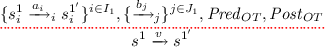
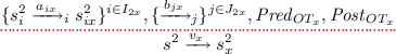
(Open Transitions). An open transition over a set $(S_i,s_{0 i}, \rightarrow _i)^{i\in I}$ of LTSs, a set J of holes with sorts $Sort_j^{j\in J}$, and a set of states $\mathcal {S}$ is a structure of the form:

Where $s, s'\in \mathcal {S}$ and for all $i\in I$, $s_i{\xrightarrow {a_i}}_i s_i^{\prime }$ is a transition of the LTS $(S_i,s_{0 i}, \rightarrow _i)$, and $\xrightarrow {b_j}_j$ is a transition of the hole j, for any action $b_j$ in the sort $Sort_j$. Pred is a predicate over the different variables of the terms, labels, and states $s_i$, $b_j$, s, v. Post is a set of equations that hold after the open transition, they are represented as a substitution of the form $\{x_k\leftarrow e_k\}^{k\in K}$ where $x_k$ are variables of $s'$, $s'_i$, and $e_k$ are expressions over the other variables of the open transition.

Example 2

An open-transition. The EnableCompL pNet of Fig. 2 has 2 controllers and 2 holes. One of its possible open-transition is:

Definition 5

(Open Automaton). An open automaton is a structure

$A = <LTS_i^{i\in I},J,\mathcal {S},s_0,\mathcal {T}>$ where:

• I and J are sets of indices,

• $LTS_i^{i\in I}$ is a family of LTSs,

• $\mathcal {S}$ is a set of states and $s_0$ an initial state among $\mathcal {S}$,

• $\mathcal {T}$ is a set of open transitions and for each $t\in \mathcal {T}$ there exist $I'$, $J'$ with $I'\subseteq I$, $J' \subseteq J$, such that t is an open transition over $LTS_i^{i\in I'}$, $J'$, and $\mathcal {S}$.

Definition 6

(States of Open pNets). A state of an open pNet is a tuple (not necessarily finite) of the states of its leaves (in which we denote tuples in structured states as $\triangleleft \ldots \triangleright$ for better readability).

For any pNet p, let $\overline{Leaves} = \langle \langle S_i,{s_i}_0, \rightarrow _i\rangle \rangle ^{i \in L}$ be the set of pLTS at its leaves, then $States(p) = \{\triangleleft s_i^{i\in L} \triangleright | \forall i\in L. s_i \in S_i\}$. A pLTS being its own single leave: $States(\langle \langle S,s_0, \rightarrow \rangle \rangle ) = \{\triangleleft s \triangleright | s \in S\}$.

The initial state is defined as: $InitState(p) = \triangleleft {{s_i}_0}^{i\in L} \triangleright$.

Predicates: Let $\langle \langle \overline{{ pNet}},\overline{S},{ SV}_k^{k\in K} \rangle \rangle$ be a pNet. Consider a synchronisation vector $SV_k$, for $k\in K$. We define a predicate ${ Pred}$ relating the actions of the involved sub-pNets and the resulting actions. This predicate verifies:

$$\begin{aligned} { Pred}(SV_k, a_i^{i\in I}, b_j^{j\in J}, v)\Leftrightarrow \begin{array}{l} \exists {(a'_i)}^{i\in I}, {(b'_j)}^{j\in J},v'.\, SV_k={(a'_i)}^{i\in I}, {(b'_j)}^{j\in J}\rightarrow v' \\ ~~\wedge \forall i\in I.\, a_i=a'_i\wedge \forall j \in J.\, b_j=b'_j \wedge v=v' \end{array} \end{aligned}$$

In any other case (if the action families do not match or if there is no valuation of variables such that the above formula can be ensured) the predicate is undefined.

This definition is not constructive but it is easy to build the predicate constructively by brute-force unification of the sub-pNets actions with the corresponding vector actions, possibly followed by a simplification step.

We build the semantics of open pNets as an open automaton where LTSs are the pLTSs at the leaves of the pNet structure, and the states are given by Definition 6. The open transitions first project the global state into states of the leaves, then apply pLTS transitions on these states, and compose them with the sort of the holes. The semantics regularly instantiates fresh variables, and uses a clone operator that clones a term replacing each variable with a fresh one.

Definition 7

(Operational Semantics of Open pNets). The semantics of a pNet p is an open automaton $A = <Leaves(p),J,\mathcal {S}, s_0, \mathcal {T}>$ where:

• J is the indices of the holes: $Holes(p)= H_j^{j\in J}$.

• $\overline{\mathcal {S}} = States(p)$ and $s_0 = InitState(p)$

• $\mathcal {T}$ is the smallest set of open transitions satisfying the rules below:

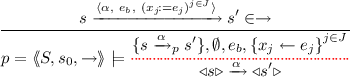
The rule for a pLTS p checks that the guard is verified and transforms assignments into post-conditions:

• Tr1:

The second rule deals with pNet nodes: for each possible synchronisation vector applicable to the rule subject, the premisses include one open transition for each sub-pNet involved, one possible action for each Hole involved, and the predicate relating these with the resulting action of the vector. A key to understand this rule is that the open transitions are expressed in terms of the leaves and holes of the pNet structure, i.e. a flatten view of the pNet: e.g. L is the index set of the Leaves, $L_k$ the index set of the leaves of one subnet, so all $L_k$ are disjoint subsets of L. Thus the states in the open transitions, at each level, are tuples including states of all the leaves of the pNet, not only those involved in the chosen synchronisation vector.

• Tr2:

Example 3

Using the operational rules to compute open-transitions In Fig. 3 we show the deduction tree used to construct and prove the open transition $OT_2$ of EnableCompL (see Example p. x). The rule uses TR1 for the $\delta$ transition of $C_3$, for the l transition of $C_4$, then combines the result using the $a_4$ vector of the bottom pNet node, and the $\underline{\delta (x)}$ vector of the top node.

Fig. 3.

Proof of transition $OT_2$ (with interaction of processes P and Q) for “P$\gg$(Q$\gg$R)”

Note that while the scenario above is expressed as a single instantiation of the possible behaviours, the constructions below are kept symbolic, and each open-transition deduced expresses a whole family of behaviours, for any possible values of the variables.

Variable Management. The variables in each synchronisation vector are considered local: for a given pNet expression, we must have fresh local variables for each occurrence of a vector (= each time we instantiate rule Tr2). Similarly the state variables of each copy of a given pLTS in the system, must be distinct, and those created for each application of Tr2 have to be fresh and all distinct. This will be implemented within the open-automaton generation algorithm, e.g. using name generation using a global counter as a suffix.

3.1 Computing and Using Open Automata

In this section we present a simple algorithm to construct the open automaton representing the behaviour of an open pNet, and we prove that under reasonable conditions this automaton is finite.

Algorithm 1

(Behavioural Semantics of Open pNets: Sketch). This is a standard residual algorithm over a set of open-automaton states, but where transitions are open transitions constructively “proven” by deduction trees.

• (1) Start with a set of unexplored states containing the initial state of the automaton, and an empty set of explored states.

• (2) While there are unexplored states:

• (2a) pick one state from the unexplored set and add it to the explored set. From this state build all possible deduction trees by application of the structural rules Tr1 and Tr2, using all applicable combinations of synchronisation vectors.

• (2b) For each of the obtained deduction trees, extract the resulting open-transition, with its predicate and Post assignments by exploring the structure of the pNet.

• (2c) Optionally, simplifying the predicate at this point may minimize the resulting transitions, or even prune the search-space.

• (2d) For each open-transition from step 2b, add the resulting state in the unexplored set if it is not already in the explored set, and add the transition in the outgoing transitions of the current state.

To have some practical interest, it is important to know when this algorithm terminates. The following theorem shows that an open-pNet with finite synchronisation sets, finitely many leaves and holes, and each pLTS at leaves having a finite number of states and (symbolic) transitions, has a finite automaton:

Theorem 2

(Finiteness of Open-Automata). Given an open pNet $\langle \langle \overline{{ pNet}},\overline{S}, { SV}_k^{k\in K}\rangle \rangle$ with leaves $pLTS_i^{i\in L}$ and holes $Hole_j^{j\in J}$, if the sets L and J are finite, if the synchronisation vectors of all pNets included in $\langle \langle \overline{{ pNet}},\overline{S}, { SV}_k^{k\in K}\rangle \rangle$ are finite, and if $\forall i \in L.\, finite{(states(pLTS_i))} \text { and } pLTS_i$ has a finite number of state variables, then Algorithm 1 terminates and produces an open automaton $\mathcal {T}$ with finitely many states and transitions.

Proof

The possible set of states of the open-automaton is the cartesian product of the states of its leaves $pLTS_i^{i\in L}$, that is finite by hypothesis. So the top-level residual loop of Algorithm 1 terminates provided each iteration terminates. The enumeration of open-transitions in step 2b is bounded by the number of applications of rules Tr2 on the structure of the pNet tree, with a finite number of synchronisation vectors applying at each node the number of global open transition is finite. Similarily rule Tr1 is applied finitely if the number of transitions of each pLTS is finite. So we get finitely many deduction trees, and open-transitions which ensures that each internal loop of Algorithm 1 terminates.    $\square$

4 Bisimulation

Now we use our symbolic operational semantics to define a notion of strong (symbolic) bisimulation.Moreover this equivalence is decidable whenever we have some decision procedure on the predicates of the action algebra.

The equivalence we need is a strong bisimulation between pNets having exactly the same Holes with the same sorts, but using a flexible matching between open transition, to accommodate comparisons between pNet expressions with different architectures. We name it FH-bisimulation, as a short cut for the “Formal Hypotheses” manipulated in the transitions, but also as a reference to the work of De Simone [1], that pioneered this idea. Formally:

Definition 9

(FH-bisimulation). Suppose that $A_1 = <L_1,J,\mathcal {S}_1, s^1_0, \mathcal {T}_1>$ and $A_2 = <L_2,J,\mathcal {S}_2,s^2_0, \mathcal {T}_2>$ are open automata where the set of holes are equal and of the same sort. Let $(s^1,s^2|{ Pred})\in \mathcal {R}$ be a relation over the sets $\mathcal {S}_1$ and $\mathcal {S}_2$ constrained by a predicate. More precisely, for any pair $(s^1,s^2)$, there is a single $(s^1,s^2|{ Pred})\in \mathcal {R}$ stating that $s^1$ and $s^2$ are related if Pred is true.

Definition 8 (FH-bisimulation).

Suppose that $A_1 = <L_1,J,\mathcal {S}_1, s^1_0, \mathcal {T}_1>$ and $A_2 = <L_2,J,\mathcal {S}_2,s^2_0, \mathcal {T}_2>$ are open automata where the set of holes are equal and of the same sort. Let $(s^1,s^2|{ Pred})\in \mathcal {R}$ be a relation over the sets $\mathcal {S}_1$ and $\mathcal {S}_2$ constrained by a predicate. More precisely, for any pair $(s^1,s^2)$, there is a single $(s^1,s^2|{ Pred})\in \mathcal {R}$ stating that $s^1$ and $s^2$ are related if Pred is true.

Then $\mathcal {R}$ is an FH-bisimulation iff for any states $s^1\in \mathcal {S}_1$ and $s^2\in \mathcal {S}_2$, $(s^1,s^2|{ Pred})\in \mathcal {R}$, we have the following:

• For any open transition OT in $\mathcal {T}_1$:

  

  there exist open transitions $OT_x^{x\in X} \subseteq \mathcal {T}_2$:

  

  such that ; and

• and symmetrically any open transition from $s^2$ in $\mathcal {T}_2$ can be covered by a set of transitions from $t^1$ in $\mathcal {T}_1$.

Two pNets are FH-bisimilar if there exist a relation between their associated automata that is an FH-bisimulation.

Classically, ${ Pred}_{target_x}\{\{\!{ Post}_{OT}\!\}\}\{\{\!{ Post}_{OT_x}\!\}\}$ applies in parallel the substitutions ${ Post}_{OT}$ and ${ Post}_{OT_x}$ (parallelism is crucial inside each ${ Post}$ set but ${ Post}_{OT}$ is independent from ${ Post}_{OT_x}$), applying the assignments of the involved rules.

Weak symbolic bisimulation can be defined in a similar way, using as invisible actions a subset of the synchronised actions defined in Sect. 2. To illustrate our approach on a simple example, let us encode the Lotos Enable operator using 2 different encodings, and prove their equivalence.

Example 4

In Fig. 1, we proposed two different open pNets encoding the expression P $\gg$ Q. While it is easy to be convinced that they are equivalent, their structures are sufficiently different to show how the FH-bisimultion works and addresses the crucial points on the proof of equivalence between operators. The open automata of these two pNets are given, together with their open transitions in Fig. 4. To illustrate the proof of bisimulation, let us build a relation:

$$\begin{aligned} R = \{ (A_0,B_0|s_0=0), (A_1,B_0|s_0=1) \} \end{aligned}$$

Fig. 4.

The two open automata

and prove that R is a strong FH-bisimulation. For each transition in each automaton, we must find a covering set of transitions, with same holes involved, and equivalent target states. Finding the matching here is trivial, and all covering sets are reduced to singleton. All proofs are pretty similar, so we only show here the details for matching (both ways) the open transitions $ot_2$ and $ot'_2$; these are the most interesting, because of the presence of the assignment.

Consider transition $ot_2$ of state $A_0$, and prove that it is covered by $ot'_2$. Let us detail the construction of the proof obligation:

The source ${ Pred}$ for $A_0$ in $ot_2$ is $s_0=0$, and $ot_2$ itself has no predicate. Then we find the condition for holes to have the same behaviours, and from that we must prove the predicate in $ot'_2$ holds, and finally the predicate of the target state $(A_1,B_0|s_0=1)$, after substitution using the assignment $\{\{\!s_0\leftarrow 1\!\}\}$, that is $1=1$. This formula (in which all variables are universally quantified) is easy to discharge.

Conversely, transition $ot'_2$ of state $B_0$ matches with $ot_2$ of $A_0$, but now the assignment is on the left hand side, and the proof goal mostly concern the triggered action as $ot_2$ has no predicate:

$s_0=0 \wedge s_0=0 \implies (\delta (y2)=\delta (x2) \wedge acc(y2)=acc(x2) \implies \underline{\delta (x2)}=\underline{\delta (y2)} \wedge 1=1)$    $\square$

Despite the simplicity of the proven equivalence, the proof of bisimulation highlights precisely the use of the different predicates. It is also important to see that all the arguments necessary for proving the equivalence are well identified and properly used, and that we really made a proof about the operator without having to refer to the behaviour of the processes that will be put in the holes. This simple example shows the expressiveness of our approach by illustrating the use of variables, assignments, controllers and sort of holes. It is straightforward to prove e.g. that the enable operator is associative, after computing the open automaton of the pNet EnableComp from Fig. 2, and a similar one representing (P>>Q)>>R). Each of the automata has 3 states and 5 open-transitions. For reasons of space we cannot show them here [15]. We can finally prove that it is decidable whether a relation is a FH-bisimulation provided the logic of the predicates is decidable.

Theorem 3

(Decidability of FH-bisimulation). Let $A_1$ and $A_2$ be finite open automata and $\mathcal {R}$ a relation over their states $\mathcal {S}_1$ and $\mathcal {S}_2$ constrained by a set of predicates. Assume that the predicates inclusion is decidable over the action algebra $\mathcal {A}_P$. Then it is decidable whether the relation $\mathcal {R}$ is a FH-bisimulation.

Proof

The principle is to consider each pair of states $(s_1,s_2)$, consider the element $(s_1,s_2|{ Pred})$ in $\mathcal {R}$; if Pred is not false we consider the (finite) set of open transition having as a conclusion. For each of them, to prove the simulation, we can consider all the transitions leaving $s_2$. Let $OT_x$ be the set of all transitions with a conclusion of the form such that the same holes are involved in the open transition and such that there exist ${ Pred}_{target_x}$ such that $(s_1',s_{2 x}'|{ Pred}_{target_x})\in R$. This gives us the predicates and Post assignments corresponding to those open transitions. We then only have to prove:

$${ Pred}\,\wedge \,{ Pred}_{OT} \Rightarrow \bigvee _{x\in X} \left( \forall j. b_j=b_{jx} \Rightarrow { Pred}_{OT_x} \wedge v\!=\!v_x \wedge { Pred}_{target_x}\{\{\!{ Post}_{OT}\!\}\}\{\{\!{ Post}_{OT_x}\!\}\}\right) $$

Which is decidable since predicates inclusion is decidable. As the set of elements in $\mathcal {R}$ is finite and the set of open transitions is finite, it is possible to check them exhaustively.    $\square$

5 Composability

The main interest of our symbolic approach is to define a method to prove properties directly on open structures, that will be preserved by any correct instantiation of the holes. In this section we define a composition operator for open pNets, and we prove that it preserves FH-bisimulation. More precisely, one can define two preservation properties, namely (1) when one hole of a pNet is filled by two bisimilar other (open) pNets; and (2) when the same hole in two bisimilar pNets are filled by the same pNet, in other words, composing a pNet with two bisimilar contexts. The general case will be obtained by transitivity of the bisimulation relation. We concentrate here on the second property, that is the most interesting.

Definition 9 (pNet Composition). An open pNet: ${ pNet}= \langle \langle { pNet}_i^{i\in I}, S_j^{j\in J}, \overline{{ SV}}\rangle \rangle$ can be (partially) filled by providing a pNets ${ pNet}'$ of the right sort to fill one of its holes. Suppose $j_0\in J$:

Theorem 4

(Context Equivalence). Consider two FH-bisimilar open pNets: ${ pNet}= \langle \langle { pNet}_i^{i\in I}, S_j^{j\in J}, \overline{{ SV}}\rangle \rangle$ and (recall they must have the same holes to be bisimilar). Let $j_0\in J$ be a hole, and Q be a pNet such that ${{\mathrm{Sort}}}(Q)=S_{j_0}$. Then ${ pNet}[Q]_{j_0}$ and ${ pNet}'[Q]_{j_0}$ are FH-bisimilar.

The proof of Theorem 4 relies on two main lemmas, dealing respectively with the decomposition of a composed behaviour between the context and the internal pNet, and with their recomposition. We start with decomposition: from one open transition of $P[Q]_{j_0}$, we exhibit corresponding behaviours of P and Q, and determine the relation between their predicates:

Lemma 1

(OT Decomposition). Let ${{\mathrm{Leaves}}}(Q)=p_l^{l\in L_Q}$; suppose:

with Q “moving” (i.e. $J\cap {{\mathrm{Holes}}}(Q)\ne \emptyset$ or $I\cap L_Q\ne \emptyset$). Then there exist $v_Q$, ${ Pred}'$, ${ Pred}''$, ${ Post}'$, ${ Post}''$ s.t.:

and ${ Pred}\{\{\!v_Q\leftarrow b_{j_0}\!\}\} =({ Pred}' \wedge { Pred}'')$, ${ Post}={ Post}'\uplus { Post}''$ where ${ Post}''$ is the restriction of ${ Post}$ over variables of ${{\mathrm{Leaves}}}(Q)$.

Proof

Consider each premise of the open transition (as constructed by rule TR2 in Definition 7). We know each premise is true for P[Q] and try to prove the equivalent premise for P. First, K and the synchronisation vector $SV_k$ are unchanged² (however $j_0$ passes from the set of subnets to the set of holes). Then $SV=clone(\alpha _j^{j\in I_k\uplus \{j_0\}\uplus J_k})$. ${{\mathrm{Leaves}}}(P[Q]_{j_0})={{\mathrm{Leaves}}}(P)\uplus {{\mathrm{Leaves}}}(Q)$. Now focus on OTs of the subnets (see footnote 2):

Only elements of $I_k$ are useful to assert the premise for reduction of P; the last one ensures (note that Q is at place $j_0$, and $I_{j_0}=I\cap L_Q$, $L_{j_0}=L_Q$):

This already ensures the second part of the conclusion if we choose (see footnote 2) $v_Q=v_{j_0}$ (${ Pred}''= { Pred}_{j_0}$). Now let $I'= \biguplus I'_m=I\setminus L_Q$, $J'=\biguplus J'_m\uplus J_k \uplus \{j_0\}=J\setminus {{\mathrm{Holes}}}(Q)\uplus \{j_0\}$; the predicate is ${ Pred}'=\bigwedge _{m\in I_k}{ Pred}_m \wedge { Pred}(SV,a_i^{i\in I_k},b_j^{j\in J_k\cup \{j_0\}},v)$ where (see footnote 2) ${ Pred}(SV,a_i^{i\in I_k},b_j^{j\in J_k},v)\Leftrightarrow \forall i\in I_k.\, \alpha _i=a_i\wedge \forall j \in J_k\cup \{j_0\}.\, \alpha _j=b_j \wedge v=\alpha '_k$. Modulo renaming of fresh variables, this is identical to the predicate that occurs in the source open transition except $\alpha _{j_0}=v_{j_0}$ has been replaced by $\alpha _{j_0}=b_{j_0}$. Thus, ${ Pred}\{\{\!v_Q\leftarrow b_{j_0}\!\}\}=({ Pred}' \wedge { Pred}'')$. Finally, Post into conditions of the context P and the pNet Q (they are builts similarly as they only deal with leaves): ${ Post}={ Post}'\uplus { Post}''$. We checked all the premises of the open transition for both P and Q.   $\square$

In general, the actions that can be emitted by Q is a subset of the possible actions of the holes, and the predicate involving $v_Q$ and the synchronisation vector is more restrictive than the one involving only the variable $b_{j_0}$. Lemma 2 is combining an open transition of P with an open transition of Q, and building a corresponding transition of $P[Q]_{j_0}$, assembling their predicates.

Lemma 2

(Open Transition Composition). Suppose $j_0\in J$ and:

Then, we have:

The proof is omitted, it is mostly similar to Lemma 1, see [15] for details. The proof of Theorem 4 exhibits a bisimulation relation for a composed system. It then uses Lemma 1 to decompose the open transition of P[Q] and obtain an open transition of P on which the FH-bisimulation property can be applied to obtain an equivalent family of open transitions of $P'$; this family is then recomposed by Lemma 2 to build open transitions of $P'[Q]$ that simulate the original one.

Proof

of (Theorem 4 ). Let ${{\mathrm{Leaves}}}(Q)=p_l^{l\in L_Q}$, ${{\mathrm{Leaves}}}(P)=p_l^{l\in L}$, ${{\mathrm{Leaves}}}(P')={p'}_l^{l\in L'}$. P is FH-bisimilar to $P'$: there is an FH-bisimulation $\mathcal {R}$ between the open automata of P and of $P'$. Consider the relation $\mathcal {R}'=\{(s_1,s_2|{ Pred})|s_1=s'_1\uplus s \wedge s_2=s'_2\uplus s \wedge s\in \mathcal {S}_Q \wedge (s_1',s_2'|{ Pred})\in \mathcal {R}\}$ where $\mathcal {S}_Q$ is the set of states of the open automaton of Q. We prove that $\mathcal {R}'$ is an open FH-bisimulation. Consider a pair of FH-bisimilar states: $(\triangleleft {s_{1 i}^{i \in L\uplus L_Q}}\triangleright ,\triangleleft {{s}_{2 i}^{i \in L'}\uplus {s}_{1 i}^{i \in L_Q}}\triangleright |{ Pred})\in \mathcal {R}'$. Consider an open transition OT of $P[Q]_{j_0}$.

Let $J'=J\setminus {{\mathrm{Holes}}}(Q) \cup \{j_0\}$. By Lemma 1 we have :

and ${ Pred}_{OT}\{\{\!v_Q\leftarrow b_{j_0}\!\}\} =({ Pred}' \wedge { Pred}'')$, ${ Post}_{OT}={ Post}'\uplus { Post}''$ (${ Post}''$ is the restriction of ${ Post}$ over variables of ${{\mathrm{Leaves}}}(Q)$). As P is FH-bisimilar to $P'$ and $(\triangleleft {s_{1 i}^{i \in L}}\triangleright ,\triangleleft {{s}_{2 i}^{i \in L'}}\triangleright |{ Pred})\in \mathcal {R}$ there is a family $OT'_x$ of open transitions of the automaton of $P'$

and $\forall x, (\triangleleft {s_{1 i}^{i\in L}}\triangleright ,\triangleleft {s_{2 i x}^{i\in L'}}\triangleright |{ Pred}_{tgt_x})\in \mathcal {R}$; and

${ Pred}\wedge { Pred}' \Rightarrow \bigvee _{x\in X} \left( \forall j\in J'. b_j=b_{jx} \Rightarrow { Pred}_{OT_x} \wedge v = v_x \wedge { Pred}_{tgt_x}\right.$ $\left. \{\{\!{ Post}'\!\}\}\{\{\!{ Post}_{OT_x}\!\}\}\right)$

By Lemma 2 (for $i\in L_Q$, $s_{2 i}=s_{1 i}$ and $s_{2 i x}=s'_{1 i}$, and for $j\in Holes(Q)$, $b_{j x}=b_j$):

Observe $J=(J\setminus {{\mathrm{Holes}}}(Q)\cup \{j_0\})\setminus \{j_0\}\cup (J\cap {{\mathrm{Holes}}}(Q))$. We verify the conditions for the FH-bisimulation between OT and $OT_x$. $\forall x, (\triangleleft {{s'}_{1 i}^{i\in L\uplus L_Q}}\triangleright ,\triangleleft {s_{2 i x}^{i\in L'\uplus L_Q}}\triangleright |{ Pred}_{tgt_x})\in \mathcal {R}'$.

The obtained formula reaches the goal except for two points:

• We need $\forall j\!\in \! J$ instead of $\forall j\!\in \! J'$ with $J'\!=\!J\!\setminus \! {{\mathrm{Holes}}}(Q) \cup \{j_0\}$ but the formula under the quantifier does not depend on $b_{j_0}$ now (thanks to the substitution). Concerning ${{\mathrm{Holes}}}(Q)$, adding quantification on new variables does not change the formula.

• We need ${ Pred}_{tgt_x}\{\{\!{ Post}_{OT}\!\}\}\{\{\!{ Post}_{OT_x}\uplus { Post}''\!\}\}$ but by Lemma 2, this is equivalent to: ${ Pred}_{tgt_x}\{\{\!Post'\uplus Post''\!\}\}\{\{\!{ Post}_{OT_x}\uplus { Post}''\!\}\}$. We can conclude by observing that ${ Pred}_{tgt_x}$ does not use any variable of Q and thus $\{\{\!Post''\!\}\}$ has no effect.    $\square$

This section proved the most interesting part of the congruence property for FH-bisimulation. The details of the additional lemmas are not only crucial for the proof but also shows that open transitions reveal to be a very powerful tool for proving properties on equivalences and systems. Indeed they show how open transitions can be composed and decomposed in the general case.

6 Conclusion and Discussion

In this paper, we built up theoretical foundation for the analysis of open parameterised automatas. pNets can be seen as a generalisation of labelled transition systems, and of generic composition systems. By studying open pNets, i.e. pNets with holes, we target not only a generalised point of view on process calculi, but also on concurrent process operators. The semantics and the bisimulation theory presented in this paper bring a strong formal background for the study of open systems and of system composition. In the past, we used pNets for building formal models of distributed component systems, and applied them in a wide range of case-studies on closed finitely instantiated distributed application. This work opens new directions that will allow us to study open parameterised systems in a systematic, and hopefully fully automatised way.

We are currently extending this work, looking at both further properties of FH-bisimulation, but also the relations with existing equivalences on closed systems. We also plan to apply open pNets to the study of complex composition operators in a symbolic way, for example in the area of parallel skeletons, or distributed algorithms. We have started developping some tool support for computing the symbolic semantics in term of open-automata. The following steps will be the development of algorithms and tools for checking FH-bisimulations, and interfacing with decision engines for predicates, typically SMT solvers. Those tools will include an algorithm that partitions the states and generates the right conditions (automatically or with user input) for checking whether two open pNets are bisimilar. Independently, it is clear that most interesting properties of such complex systems will not be provable by strong bisimulation. Next steps will include the investigation of weak versions of the FH-bisimulation, using the notion of synchronised actions mentionned in the paper.

References

De Simone, R.: Higher-level synchronising devices in MEIJE-SCCS. Theor. Comput. Sci. 37, 245–267 (1985)
Larsen, K.G.: A context dependent equivalence between processes. Theor. Comput. Sci. 49, 184–215 (1987)
Hennessy, M., Lin, H.: Symbolic bisimulations. Theor. Comput. Sci. 138(2), 353–389 (1995)
Lin, H.: Symbolic transition graph with assignment. In: Sassone, V., Montanari, U. (eds.) CONCUR 1996. LNCS, vol. 1119, pp. 50–65. Springer, Heidelberg (1996)
Hennessy, M., Rathke, J.: Bisimulations for a calculus of broadcasting systems. Theor. Comput. Sci. 200(1–2), 225–260 (1998)
Arnold, A.: Synchronised behaviours of processes and rational relations. Acta Informatica 17, 21–29 (1982)
Henrio, L., Madelaine, E., Zhang, M.: pNets: an expressive model for parameterisednetworks of processes. In: 23rd Euromicro International Conference on Parallel, Distributed, and Network-Based Processing (PDP 2015) (2015)
Cansado, A., Madelaine, E.: Specification and verification for grid component-based applications: from models to tools. In: de Boer, F.S., Bonsangue, M.M., Madelaine, E. (eds.) FMCO 2008. LNCS, vol. 5751, pp. 180–203. Springer, Heidelberg (2009)
Henrio, L., Kulankhina, O., Li, S., Madelaine, E.: Integrated environment for verifying and running distributed components. In: Stevens, P. (ed.) FASE 2016. LNCS, vol. 9633, pp. 66–83. Springer, Heidelberg (2016). doi:10.1007/978-3-662-49665-7_5
Rensink, A.: Bisimilarity of open terms. In: Expressiveness in Languages for Concurrency (1997)
Deng, Y.: Algorithm for verifying strong open bisimulation in \(\pi \) calculus. J. Shanghai Jiaotong Univ. 2, 147–152 (2001)
Bultan, T., Gerber, R., Pugh, W.: Symbolic model checking of infinite state systems using presburger arithmetic. In: Grumberg, O. (ed.) CAV 1997. LNCS, vol. 1254, pp. 400–411. Springer, Heidelberg (1997)
Clarke, E.M., Grumberg, O., Jha, S.: Verifying parameterized networks. ACM Trans. Program. Lang. Syst. 19(5), 726–750 (1997)
Milner, R.: Communication and Concurrency. International Series in Computer Science. Prentice-Hall, Englewood Cliffs (1989). SU Fisher Research 511/24
Henrio, L., Madelaine, E., Zhang, M.: A theory for the composition of concurrent processes - extended version. Rapport de recherche RR-8898, INRIA, April 2016
Author information
Authors and Affiliations
Corresponding author
Editor information
Editors and Affiliations
Rights and permissions
Copyright information
© 2016 IFIP International Federation for Information Processing
About this paper
Cite this paper
Henrio, L., Madelaine, E., Zhang, M. (2016). A Theory for the Composition of Concurrent Processes. In: Albert, E., Lanese, I. (eds) Formal Techniques for Distributed Objects, Components, and Systems. FORTE 2016. Lecture Notes in Computer Science(), vol 9688. Springer, Cham. https://doi.org/10.1007/978-3-319-39570-8_12
Download citation
DOI: https://doi.org/10.1007/978-3-319-39570-8_12
Published:
Publisher Name: Springer, Cham
Print ISBN: 978-3-319-39569-2
Online ISBN: 978-3-319-39570-8
eBook Packages: Computer ScienceComputer Science (R0)