Secure Multi-party Quantum Computation with a Dishonest Majority

Abstract

The cryptographic task of secure multi-party (classical) computation has received a lot of attention in the last decades. Even in the extreme case where a computation is performed between k mutually distrustful players, and security is required even for the single honest player if all other players are colluding adversaries, secure protocols are known. For quantum computation, on the other hand, protocols allowing arbitrary dishonest majority have only been proven for $k=2$. In this work, we generalize the approach taken by Dupuis, Nielsen and Salvail (CRYPTO 2012) in the two-party setting to devise a secure, efficient protocol for multi-party quantum computation for any number of players k, and prove security against up to $k-1$ colluding adversaries. The quantum round complexity of the protocol for computing a quantum circuit of $\{\mathsf {CNOT}, \mathsf {T} \}$ depth d is $O(k \cdot (d + \log n))$, where n is the security parameter. To achieve efficiency, we develop a novel public verification protocol for the Clifford authentication code, and a testing protocol for magic-state inputs, both using classical multi-party computation.

1 Introduction

In secure multi-party computation (MPC), two or more players want to jointly compute some publicly known function on their private data, without revealing their inputs to the other players. Since its introduction by Yao [Yao82], MPC has been extensively developed in different setups, leading to applications of both theoretical and practical interest (see, e.g., [CDN15] for a detailed overview).

With the emergence of quantum technologies, it becomes necessary to understand its consequences in the field of MPC. First, classical MPC protocols have to be secured against quantum attacks. But also, the increasing number of applications where quantum computational power is desired motivates protocols enabling multi-party quantum computation (MPQC) on the players’ private (possibly quantum) data. In this work, we focus on the second task. Informally, we say a MPQC protocol is secure if the following two properties hold: 1. Dishonest players gain no information about the honest players’ private inputs. 2. If the players do not abort the protocol, then at the end of the protocol they share a state corresponding to the correct computation applied to the inputs of honest players (those that follow the protocol) and some choice of inputs for the dishonest players.

MPQC was first studied by Crépeau, Gottesman and Smith [CGS02], who proposed a k-party protocol based on verifiable secret sharing that is information-theoretically secure, but requires the assumption that at most k/6 players are dishonest. The fraction k/6 was subsequently improved to ${<}k/2$ [BOCG+06] which is optimal for secret-sharing-based protocols due to no-cloning. The case of a dishonest majority was thus far only considered for $k=2$ parties, where one of the two players can be dishonest [DNS10, DNS12, KMW17]¹. These protocols are based on different cryptographic techniques, in particular quantum authentication codes in conjunction with classical MPC [DNS10, DNS12] and quantum-secure bit commitment and oblivious transfer [KMW17].

In this work, we propose the first secure MPQC protocol for any number k of players in the dishonest majority setting, i.e., the case with up to $k-1$ colluding adversarial players.² We remark that our result achieves composable security, which is proven according to the standard ideal-vs.-real definition. Like the protocol of [DNS12], on which our protocol is built, our protocol assumes a classical MPC that is secure against a dishonest majority, and achieves the same security guarantees as this classical MPC. In particular, if we instantiate this classical MPC with an MPC in the pre-processing model (see [BDOZ11, DPSZ12, KPR18, CDE+18]), our construction yields a MPQC protocol consisting of a classical “offline” phase used to produce authenticated shared randomness among the players, and a second “computation” phase, consisting of our protocol, combined with the “computation” phase of the classical MPC. The security of the “offline” phase requires computational assumptions, but assuming no attack was successful in this phase, the second phase has information-theoretic security.

1.1 Prior Work

Our protocol builds on the two-party protocol of Dupuis, Nielsen, and Salvail [DNS12], which we now describe in brief. The protocol uses a classical MPC protocol, and involves two parties, Alice and Bob, of whom at least one is honestly following the protocol. Alice and Bob encode their inputs using a technique called swaddling: if Alice has an input qubit $\left| \psi \right\rangle$, she first encodes it using the n-qubit Clifford code (see Definition 2.5), resulting in $A(\left| 0^n\right\rangle \otimes \left| \psi \right\rangle )$, for some random $(n+1)$-qubit Clifford A sampled by Alice, where n is the security parameter. Then, she sends the state to Bob, who puts another encoding on top of Alice’s: he creates the “swaddled” state $B(A(\left| 0^n\right\rangle \otimes \left| \psi \right\rangle ) \otimes \left| 0^n\right\rangle )$ for some random $(2n+1)$-qubit Clifford B sampled by Bob. This encoded state consists of $2n+1$ qubits, and the data qubit $\left| \psi \right\rangle$ sits in the middle.

If Bob wants to test the state at some point during the protocol, he simply needs to undo the Clifford B, and test that the last n qubits (called traps) are $\left| 0\right\rangle$. However, if Alice wants to test the state, she needs to work together with Bob to access her traps. Using classical multi-party computation, they jointly sample a random $(n+1)$-qubit Clifford $B'$ which is only revealed to Bob, and compute a Clifford $T := (\mathbb {I} ^{\otimes n} \otimes B')(A^{\dagger } \otimes \mathbb {I} ^{\otimes n})B^{\dagger }$ that is only revealed to Alice. Alice, who will not learn any relevant information about B or $B'$, can use T to “flip” the swaddle, revealing her n trap qubits for measurement. After checking that the first n qubits are $\left| 0\right\rangle$, she adds a fresh $(2n+1)$-qubit Clifford on top of the state to re-encode the state, before computation can continue.

Single-qubit Clifford gates are performed simply by classically updating the inner key: if a state is encrypted with Cliffords BA, updating the decryption key to $BAG^\dagger$ effectively applies the gate G. In order to avoid that the player holding the inner key B skips this step, both players keep track of their keys using a classical commitment scheme. This can be encapsulated in the classical MPC, which we can assume acts as a trusted third party with a memory [BOCG+06].

$\mathsf {CNOT}$ operations and measurements are slightly more involved, and require both players to test the authenticity of the relevant states several times. Hence, the communication complexity scales linearly with the number of CNOTs and measurements in the circuit.

Finally, to perform $\mathsf {T}$ gates, the protocol makes use of so-called magic states. To obtain reliable magic states, Alice generates a large number of them, so that Bob can test a sufficiently large fraction. He decodes them (with Alice’s help), and measures whether they are in the expected state. If all measurements succeed, Bob can be sufficiently certain that the untested (but still encoded) magic states are in the correct state as well.

Extending two-party computation to multi-party computation. A natural question is how to lift a two-party computation protocol to a multi-party computation protocol. We discuss some of the issues that arise from such an approach, making it either infeasible or inefficient.

Composing ideal functionalities. The first naive idea would be trying to split the k players in two groups and make the groups simulate the players of a two-party protocol, whereas internally, the players run $\frac{k}{2}$-party computation protocols for all steps in the two-party protocol. Those $\frac{k}{2}$-party protocols are in turn realized by running $\frac{k}{4}$-party protocols, etc., until at the lowest level, the players can run actual two-party protocols.

Trying to construct such a composition in a black-box way, using the ideal functionality of a two-party protocol, one immediately faces a problem: at the lower levels, players learn intermediate states of the circuit, because they receive plaintext outputs from the ideal two-party functionality. This would immediately break the privacy of the protocol. If, on the other hand, we require the ideal two-party functionality to output encoded states instead of plaintexts, then the size of the ciphertext will grow at each level. The overhead of this approach would be $O(n^{\log k})$, where $n \geqslant k$ is the security parameter of the encoding, which would make this overhead super-polynomial in the number of players.

Naive extension of DNS to multi-party. One could also try to extend [DNS12] to multiple parties by adapting the subprotocols to work for more than two players. While this approach would likely lead to a correct and secure protocol for k parties, the computational costs of such an extension could be high.

First, note that in such an extension, each party would need to append n trap qubits to the encoding of each qubit, causing an overhead in the ciphertext size that is linear in k. Secondly, in this naive extension, the players would need to create $\varTheta (2^k)$ magic states for $\mathsf {T}$ gates (see Sect. 2.5), since each party would need to sequentially test at least half of the ones approved by all previous players.

Notice that in both this extension and our protocol, a state has to pass by the honest player (and therefore all players) in order to be able to verify that it has been properly encoded.

1.2 Our Contributions

Our protocol builds on the work of Dupuis, Nielsen, and Salvail [DNS10, DNS12], and like it, assumes a classical MPC, and achieves the same security guarantees as this classical MPC. In contrast to a naive extension of [DNS12], requiring $\varTheta (2^k)$ magic states, the complexity of our protocol, when considering a quantum circuit that contains, among other gates, g gates in $\{\mathsf {CNOT}, \mathsf {T} \}$ and acts on w qubits, scales as $O((g+w)k)$.

In order to efficiently extend the two-party protocol of [DNS12] to a general k-party protocol, we make two major alterations to the protocol:

Public authentication test. In [DNS12], given a security parameter n, each party adds n qubits in the state $\left| 0\right\rangle$ to each input qubit in order to authenticate it. The size of each ciphertext is thus $2n+1$. The extra qubits serve as check qubits (or “traps”) for each party, which can be measured at regular intervals: if they are non-zero, somebody tampered with the state.

In a straightforward generalization to k parties, the ciphertext size would become $kn+1$ per input qubit, putting a strain on the computing space of each player. In our protocol, the ciphertext size is constant in the number of players: it is usually $n+1$ per input qubit, temporarily increasing to $2n+1$ for qubits that are involved in a computation step. As an additional advantage, our protocol does not require that all players measure their traps every time a state needs to be checked for its authenticity.

To achieve this smaller ciphertext size, we introduce a public authentication test. Our protocol uses a single, shared set of traps for each qubit. If the protocol calls for the authentication to be checked, the player that currently holds the state cannot be trusted to simply measure those traps. Instead, she temporarily adds extra trap qubits, and fills them with an encrypted version of the content of the existing traps. Now she measures only the newly created ones. The encryption ensures that the measuring player does not know the expected measurement outcome. If she is dishonest and has tampered with the state, she would have to guess a random n-bit string, or be detected by the other players. We design a similar test that checks whether a player has honestly created the first set of traps for their input at encoding time.

Efficient magic-state preparation. For the computation of non-Clifford gates, the [DNS12] protocol requires the existence of authenticated “magic states”, auxiliary qubits in a known and fixed state that aid in the computation. In a two-party setting, one of the players can create a large number of such states, and the other player can, if he distrusts the first player, test a random subset of them to check if they were honestly initialized. Those tested states are discarded, and the remaining states are used in the computation.

In a k-party setting, such a “cut-and-choose” strategy where all players want to test a sufficient number of states would require the first party to prepare an exponential number (in k) of authenticated magic states, which quickly gets infeasible as the number of players grows. Instead, we need a testing strategy where dishonest players have no control over which states are selected for testing. We ask the first player to create a polynomial number of authenticated magic states. Subsequently, we use classical MPC to sample random, disjoint subsets of the proposed magic states, one for each player. Each player continues to decrypt and test their subset of states. The random selection process implies that, conditioned on the test of the honest player(s) being successful, the remaining registers indeed contain encrypted states that are reasonably close to magic states. Finally, we use standard magic-state distillation to obtain auxiliary inputs that are exponentially close to magic states.

1.3 Overview of the Protocol

We describe some details of the k-player quantum MPC protocol for circuits consisting of classically-controlled Clifford operations and measurements. Such circuits suffice to perform Clifford computation and magic-state distillation, so that the protocol can be extended to arbitrary circuits using the technique described above. The protocol consists of several subprotocols, of which we highlight four here: input encoding, public authentication test, single-qubit gate application, and CNOT application. In the following description, the classical MPC is treated as a trusted third party with memory³. The general idea is to first ensure that initially all inputs are properly encoded into the Clifford authentication code, and to test the encoding after each computation step that exposes the encoded qubit to an attack. During the protocol, the encryption keys for the Clifford authentication code are only known to the MPC.

Input encoding. For an input qubit $\left| \psi \right\rangle$ of player i, the MPC hands each player a circuit for a random $(2n+1)$-qubit Clifford group element. Now player i appends 2n “trap” qubits initialized in the $\left| 0\right\rangle$-state and applies her Clifford. The state is passed around, and all other players apply their Clifford one-by-one, resulting in a Clifford-encoded qubit $F(\left| \psi \right\rangle \left| 0^{2n}\right\rangle )$ for which knowledge of the encoding key F is distributed among all players. The final step is our public authentication test, which is used in several of the other subprotocols as well. Its goal is to ensure that all players, including player i, have honestly followed the protocol.

The public authentication test (details). The player holding the state $F(\left| \psi \right\rangle \left| 0^{2n}\right\rangle )$ (player i) will measure n out of the 2n trap qubits, which should all be 0. To enable player i to measure a random subset of n of the trap qubits, the MPC could instruct her to apply $(E\otimes \mathsf{X}^r)(\mathbb {I}\otimes U_\pi ) F^{\dagger }$ to get $E(\left| \psi \right\rangle \left| 0^n\right\rangle )\otimes \left| r\right\rangle$, where $U_\pi$ permutes the 2n trap qubits by a random permutation $\pi$, and E is a random $(n+1)$ qubit Clifford, and $r\in \{0,1\}^n$ is a random string. Then when player i measures the last n trap qubits, if the encoding was correct, she will obtain r and communicate this to the MPC. However, this only guarantees that the remaining traps are correct up to polynomial error.

To get a stronger guarantee, we replace the random permutation with an element from the sufficiently rich yet still efficiently samplable group of invertible transformations over $\mathbb {F}^{2n}$, $\mathrm {GL}(2n,\mathbb {F}_2)$. An element $g\in \mathrm {GL}(2n,\mathbb {F}_2)$ maybe be viewed as a unitary $U_g$ acting on computational basis states as $U_g\left| x\right\rangle =\left| gx\right\rangle$ where $x \in \{0,1\}^{2n}$. In particular, $U_g\left| 0^{2n}\right\rangle =\left| 0^{2n}\right\rangle$, so if all traps are in the state $\left| 0\right\rangle$, applying $U_g$ does not change this, whereas for non-zero x, $U_g\left| x\right\rangle =\left| x'\right\rangle$ for a random $x'\in \{0,1\}^{2n}$. Thus the MPC instructs player i to apply $(E\otimes \mathsf{X}^r)(\mathbb {I}\otimes U_g) F^{\dagger }$ to the state $F(\left| \psi \right\rangle \left| 0^{2n}\right\rangle )$, then measure the last n qubits and return the result, aborting if it is not r. Crucially, $(E\otimes \mathsf{X}^r)(\mathbb {I}\otimes U_g) F^{\dagger }$ is given as an element of the Clifford group, hiding the structure of the unitary and, more importantly, the values of r and g. So if player i is dishonest and holds a corrupted state, she can only pass the MPC’s test by guessing r. If player i correctly returns r, we have the guarantee that the remaining state is a Clifford-authenticated qubit with n traps, $E(\left| \psi \right\rangle \left| 0^n\right\rangle )$, up to exponentially small error.

Single-qubit Clifford gate application. As in [DNS12], this is done by simply updating encryption key held by the MPC: If a state is currently encrypted with a Clifford E, decrypting with a “wrong” key $EG^\dagger$ has the effect of applying G to the state.

CNOT application. Applying a CNOT gate to two qubits is slightly more complicated: as they are encrypted separately, we cannot just implement the CNOT via a key update like in the case of single qubit Clifford gates. Instead, we bring the two encoded qubits together, and then run a protocol that is similar to input encoding using the $(2n+2)$-qubit register as “input”, but using 2n additional traps instead of just n, and skipping the final authentication-testing step. The joint state now has $4n+2$ qubits and is encrypted with some Clifford F only known to the MPC. Afterwards, $\mathsf {CNOT}$ can be applied via a key update, similarly to single-qubit Cliffords. To split up the qubits again afterwards, the executing player applies $(E_1 \otimes E_2)F^{\dagger }$, where $E_1$ and $E_2$ are freshly sampled by the MPC. The two encoded qubits can then be tested separately using the public authentication test.

1.4 Open Problems

Our results leave a number of exciting open problems to be addressed in future work. Firstly, the scope of this work was to provide a protocol that reduces the problem of MPQC to classical MPC in an information-theoretically secure way. Hence we obtain an information-theoretically secure MPQC protocol in the preprocessing model, leaving the post-quantum secure instantiation of the latter as an open problem.

Another class of open problems concerns applications of MPQC. For instance, classically, MPC can be used to devise zero-knowledge proofs [IKOS09] and digital signature schemes [CDG+17].

An interesting open question concerning our protocol more specifically is whether the CNOT sub-protocol can be replaced by a different one that has round complexity independent of the total number of players, reducing the quantum round complexity of the whole protocol. We also wonder if it is possible to develop more efficient protocols for narrower classes of quantum computation, instead of arbitrary (polynomial-size) quantum circuits.

Finally, it would be interesting to investigate whether the public authentication test we use can be leveraged in protocols for specific MPC-related tasks like oblivious transfer.

1.5 Outline

In Sect. 2, we outline the necessary preliminaries and tools we will make use of in our protocol. In Sect. 3, we give a precise definition of MPQC. In Sect. 4, we describe how players encode their inputs to setup for computation in our protocol. In Sect. 5 we describe our protocol for Clifford circuits, and finally, in Sect. 6, we show how to extend this to universal quantum circuits in Clifford+$\mathsf {T}$ .

2 Preliminaries

2.1 Notation

We assume familiarity with standard notation in quantum computation, such as (pure and mixed) quantum states, the Pauli gates $\mathsf {X}$ and $\mathsf {Z}$, the Clifford gates $\mathsf {H}$ and $\mathsf {CNOT}$, the non-Clifford gate $\mathsf {T}$, and measurements.

We work in the quantum circuit model, with circuits C composed of elementary unitary gates (of the set Clifford+$\mathsf {T}$), plus computational basis measurements. We consider those measurement gates to be destructive, i.e., to destroy the post-measurement state immediately, and only a classical wire to remain. Since subsequent gates in the circuit can still classically control on those measured wires, this point of view is as general as keeping the post-measurement states around.

For a set of quantum gates $\mathcal {G}$, the $\mathcal {G}$-depth of a quantum circuit is defined as the minimal number of layers such that in every layer, gates from $\mathcal {G}$ do not act on the same qubit.

For two circuits $C_1$ and $C_2$, we write $C_2 \circ C_1$ for the circuit that consists of executing $C_1$, followed by $C_2$. Similarly, for two protocols $\varPi _1$ and $\varPi _2$, we write $\varPi _2 \diamond \varPi _1$ for the execution of $\varPi _1$, followed by the execution of $\varPi _2$.

We use capital letters for both quantum registers (M, R, S, $T, \dots$) and unitaries (A, B, U, V, $W, \dots$). We write |R| for the dimension of the Hilbert space in a register R. The registers in which a certain quantum state exists, or on which some map acts, are written as gray superscripts, whenever it may be unclear otherwise. For example, a unitary U that acts on register A, applied to a state $\rho$ in the registers AB, is written as , where the registers $U^\dagger$ acts on can be determined by finding the matching U and reading the grey subscripts. Note that we do not explicitly write the operation with which U is in tensor product. The gray superscripts are purely informational, and do not signify any mathematical operation. If we want to denote, for example, a partial trace of the state , we use the conventional notation $\rho _A$.

For an n-bit string $s = s_1s_2\cdots s_n$, define $U^s := U^{s_1} \otimes U^{s_2} \otimes \cdots \otimes U^{s_n}$. For an n-element permutation $\pi \in S_n$, define $P_{\pi }$ to be the unitary that permutes n qubits according to $\pi$:

$$\begin{aligned} P_\pi \left| \psi _1\right\rangle ...\left| \psi _n\right\rangle = \left| \psi _{\pi (1)}\right\rangle ...\left| \psi _{\pi (n)}\right\rangle . \end{aligned}$$

We use [k] for the set $\{1,2,\dots ,k\}$. For a projector $\varPi$, we write $\overline{\varPi }$ for its complement $\mathbb {I}- \varPi$. We use for the fully mixed state on the register R.

Write GL(n, F) for the general linear group of degree n over a field F. We refer to the Galois field of two elements as $\mathbb {F}_2$, the n-qubit Pauli group as $\mathscr {P}_n$, and the n-qubit Clifford group as $\mathscr {C}_n$. Whenever a protocol mandates handing an element from one of these groups, or more generally, a unitary operation, to an agent, we mean that a (classical) description of the group element is given, e.g. as a normal-form circuit.

Finally, for a quantum operation that may take multiple rounds of inputs and outputs, for example an environment $\mathcal {E}$ interacting with a protocol $\varPi$, we write $\mathcal {E}\leftrightarrows \varPi$ for the final output of $\mathcal {E}$ after the entire interaction.

2.2 Classical Multi-party Computation

At this point, we are unaware of any formal analysis of the post-quantum security of existing classical multi-party computation schemes. Establishing full post-quantum security of classical multi-party computation is outside the scope of this paper, but we discuss some possible directions in the full version. For the purpose of this paper, we assume that a post-quantum secure classical multi-party computation is available.

Throughout this paper, we will utilize the following ideal MPC functionality as a black box:

Definition 2.1

(Ideal classical k-party stateful computation with abort). Let $f_1, ..., f_k$ and $f_S$ be public classical deterministic functions on $k+2$ inputs. Let a string s represent the internal state of the ideal functionality. (The first time the ideal functionality is called, s is empty.) Let $A \subsetneq [k]$ be a set of corrupted players.

• 1. Every player $i \in [k]$ chooses an input $x_i$ of appropriate size, and sends it (securely) to the trusted third party.

• 2. The trusted third party samples a bit string r uniformly at random.

• 3. The trusted third party computes $f_i(s,x_1, ..., x_k,r)$ for all $i \in [k] \cup \{S\}$.

• 4. For all $i \in A$, the trusted third party sends $f_i(s,x_1, ..., x_k,r)$ to player i.

• 5. All $i \in A$ respond with a bit $b_i$, which is 1 if they choose to abort, or 0 otherwise.

• 6. If $b_j = 0$ for all j, the trusted third party sends $f_i(s,x_1, ..., x_k,r)$ to the other players $i \in [k]\backslash A$ and stores $f_S(s,x_1, ..., x_k,r)$ in an internal state register (replacing s). Otherwise, he sends an abort message to those players.

2.3 Pauli Filter

In our protocol, we use a technique which alters a channel that would act jointly on registers S and T, so that its actions on S are replaced by a flag bit into a separate register. The flag is set to 0 if the actions on S belong to some set $\mathcal {P}$, or to 1 otherwise. This way, the new channel “filters” the allowed actions on S.

Definition 2.2

(Pauli filter). For registers S and T with $|T| > 0$, let be a unitary, and let $\mathcal {P}\subseteq \left( \{0,1\}^{\log |S|}\right) ^2$ contain pairs of bit strings. The $\mathcal {P}$-filter of U on register S, denoted $\mathsf {PauliFilter}_{\mathcal {P}}^{S} (U)$, is the map $T \rightarrow TF$ (where F is some single-qubit flag register) that results from the following operations:

• 1. Initialize two separate registers S and $S'$ in the state , where $\left| \varPhi \right\rangle := \left( \frac{1}{\sqrt{2}}(\left| 00\right\rangle + \left| 11\right\rangle )\right) ^{\otimes \log |S|}$. Half of each pair is stored in S, the other in $S'$.

• 2. Run U on ST.

• 3. Measure $SS'$ with the projective measurement $\{\varPi , \mathbb {I}- \varPi \}$ for

  

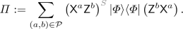
  If the outcome is $\varPi$, set the F register to . Otherwise, set it to .

The functionality of the Pauli filter becomes clear in the following lemma, which we prove in the full version by straightforward calculation:

Lemma 2.3

For registers S and T with $|T| > 0$, let be a unitary, and let $\mathcal {P}\subseteq \left( \{0,1\}^{\log |S|}\right) ^2$. Write . Then $\mathsf {PauliFilter}_{\mathcal {P}}^{S} (U)$ equals the map

A special case of the Pauli filter for $\mathcal {P}= \{(0^{\log |S|},0^{\log |S|})\}$ is due to Broadbent and Wainewright [BW16]. This choice of $\mathcal {P}$ represents only identity: the operation $\mathsf {PauliFilter}_{\mathcal {P}}^{}$ filters out any components of U that do not act as identity on S. We will denote this type of filter with the name $\mathsf {IdFilter}^{}$.

In this work, we will also use $\mathsf {XFilter}^{S} (U)$, which only accepts components of U that act trivially on register S in the computational basis. It is defined by choosing $\mathcal {P}= \{0^{\log |S|}\} \times \{0,1\}^{\log |S|}$.

Finally, we note that the functionality of the Pauli filter given in Definition 2.2 can be generalized, or weakened in a sense, by choosing a different state than . In this work, we will use the $\mathsf {ZeroFilter}^{S} (U)$, which initializes $SS'$ in the state $\left| 00\right\rangle ^{\log |S|}$, and measures using the projector . It filters U by allowing only those Pauli operations that leave the computational-zero state (but not necessarily any other computational-basis states) unaltered:

where we abbreviate $U_a := \sum _b U_{a,b}$. Note that for $\mathsf {ZeroFilter}^{S} (U)$, the extra register $S'$ can also be left out.

2.4 Clifford Authentication Code

The protocol presented in this paper will rely on quantum authentication. The players will encode their inputs using a quantum authentication code to prevent the other, potentially adversarial, players from making unauthorized alterations to their data. That way, they can ensure that the output of the computation is in the correct logical state.

A quantum authentication code transforms a quantum state (the logical state or plaintext) into a larger quantum state (the physical state or ciphertext) in a way that depends on a secret key. An adversarial party that has access to the ciphertext, but does not know the secret key, cannot alter the logical state without being detected at decoding time.

More formally, an authentication code consists of an encoding map and a decoding map , for a secret key k, which we usually assume that the key is drawn uniformly at random from some key set $\mathcal {K}$. The message register M is expanded with an extra register T to accommodate for the fact that the ciphertext requires more space than the plaintext.

An authentication code is correct if $\mathsf {Dec} _k \circ \mathsf {Enc} _k = \mathbb {I}$. It is secure if the decoding map rejects (e.g., by replacing the output with a fixed reject symbol $\bot$) whenever an attacker tried to alter an encoded state:

Definition 2.4

(Security of authentication codes [DNS10]). Let be a quantum authentication scheme for k in a key set $\mathcal {K}$. The scheme is $\varepsilon$-secure if for all CPTP maps acting on the ciphertext and a side-information register R, there exist CP maps $\varLambda _{\mathsf {acc}}$ and $\varLambda _{\mathsf {rej}}$ such that $\varLambda _{\mathsf {acc}} + \varLambda _{\mathsf {rej}}$ is trace-preserving, and for all :

A fairly simple but powerful authentication code is the Clifford code:

Definition 2.5

(Clifford code [ABOE10]). The n-qubit Clifford code is defined by a key set $\mathscr {C}_{n+1}$, and the encoding and decoding maps for a $C \in \mathscr {C}_{n+1}$:

Note that, from the point of view of someone who does not know the Clifford key C, the encoding of the Clifford code looks like a Clifford twirl (see the full version) of the input state plus some trap states.

We prove the security of the Clifford code in the full version.

2.5 Universal Gate Sets

It is well known that if, in addition to Clifford gates, we are able to apply any non-Clifford gate G, then we are able to achieve universal quantum computation. In this work, we focus on the non-Clifford $\mathsf {T}$ gate (or $\pi /8$ gate).

In several contexts, however, applying non-Clifford gates is not straightforward for different reasons: common quantum error-correcting codes do not allow transversal implementation of non-Clifford gates, the non-Clifford gates do not commute with the quantum one-time pad and, more importantly in this work, neither with the Clifford encoding.

In order to concentrate the hardness of non-Clifford gates in an offline pre-processing phase, we can use techniques from computation by teleportation if we have so-called magic states of the form $\left| \mathsf {T} \right\rangle := \mathsf {T} \left| +\right\rangle$. Using a single copy of this state as a resource, we are able to implement a $\mathsf {T}$ gate using the circuit in Fig. 1. The circuit only requires (classically controlled) Clifford gates.

Fig. 1.

Using a magic state $\left| \mathsf T\right\rangle =\mathsf {T}\left| +\right\rangle$ to implement a $\mathsf {T}$ gate.

The problem is how to create such magic states in a fault-tolerant way. Bravyi and Kitaev [BK05] proposed a distillation protocol that allows to create states that are $\delta$-close to true magic states, given $\mathrm {poly}(\log (1/{\delta }))$ copies of noisy magic-states. Let $\left| \mathsf {T}^\bot \right\rangle =\mathsf {T}\left| -\right\rangle$. Then we have:

Theorem 2.6

(Magic-state distillation [BK05]). There exists a circuit of CNOT-depth $d_{\mathrm {distill}}(n) \leqslant O(\log (n))$ consisting of $p_{\mathrm {distill}}(n) \leqslant \mathsf {poly}\left( n\right)$ many classically controlled Cliffords and computational-basis measurements such that for any $\varepsilon < \frac{1}{2}\left( 1-\sqrt{3/7}\right)$, if $\rho$ is the output on the first wire using input

(1)

then ${1-\left\langle \mathsf {T}\right| \rho \left| \mathsf {T}\right\rangle }\leqslant O\left( (5\varepsilon )^{n^c}\right)$, where $c=(\log _2 30)^{-1}\approx 0.2$.

As we will see in Sect. 6, our starting point is a bit different from the input state required by Theorem 2.6. We now present a procedure that will allow us to prepare the states necessary for applying Theorem 2.6 (see Circuit 2.8). We prove Lemma 2.7 in the full version.

Lemma 2.7

Let $V_{LW}=\mathrm {span}\{P_\pi (\left| \mathsf {T} \right\rangle ^{\otimes m-w}\left| \mathsf {T} ^\perp \right\rangle ^{w}):w \leqslant \ell , \pi \in S_m\}$, and let $\varPi _{LW}$ be the orthogonal projector onto $V_{LW}$. Let $\varXi$ denote the CPTP map induced by Circuit 2.8. If $\rho$ is an m-qubit state such that ${\mathop Tr }(\varPi _{LW}\rho )\geqslant 1-\varepsilon$, then

$$\left\| \,\varXi (\rho )-(\left| \mathsf {T} \right\rangle \left\langle \mathsf {T} \right| )^{\otimes t}\,\right\| _1\leqslant O\left( m\sqrt{t}\left( \frac{\ell }{m}\right) ^{O((m/t)^c/2)}+\varepsilon \right) ,$$

for some constant $c>0$.

Circuit 2.8 (Magic-state distillation). Given an m-qubit input state and a parameter $t < m$:

• 1. To each qubit, apply $\hat{\mathsf {Z}}:=\mathsf {PX}$ with probability $\frac{1}{2}$.

• 2. Permute the qubits by a random $\pi \in S_m$.

• 3. Divide the m qubits into t blocks of size m/t, and apply magic-state distillation from Theorem 2.6 to each block.

Remark 2.9

Circuit 2.8 can be implemented with (classically controlled) Clifford gates and measurements in the computational basis.

3 Multi-party Quantum Computation: Definitions

In this section, we describe the ideal functionality we aim to achieve for multi-party quantum computation (MPQC) with a dishonest majority. As noted in Sect. 2.2, we cannot hope to achieve fairness: therefore, we consider an ideal functionality with the option for the dishonest players to abort.

Definition 3.1

(Ideal quantum k-party computation with abort). Let C be a quantum circuit on $W \in \mathbb {N}_{>0}$ wires. Consider a partition of the wires into the players’ input registers plus an ancillary register, as $[W] = R_1^{\mathsf {in}} \sqcup \cdots \sqcup R_k^{\mathsf {in}} \sqcup R^{\mathsf {ancilla}}$, and a partition into the players’ output registers plus a register that is discarded at the end of the computation, as $[W] = R_1^{\mathsf {out}} \sqcup \cdots \sqcup R_k^{\mathsf {out}} \sqcup R^{\mathsf {discard}}$. Let $I_A \subsetneq [k]$ be a set of corrupted players.

• 1. Every player $i \in [k]$ sends the content of $R_i^{\mathsf {in}}$ to the trusted third party.

• 2. The trusted third party populates $R^{\mathsf {ancilla}}$ with computational-zero states.

• 3. The trusted third party applies the quantum circuit C on the wires [W].

• 4. For all $i \in I_A$, the trusted third party sends the content of $R_i^{\mathsf {out}}$ to player i.

• 5. All $i \in I_A$ respond with a bit $b_i$, which is 1 if they choose to abort, or 0 otherwise.

• 6. If $b_i = 0$ for all i, the trusted third party sends the content of $R_i^{\mathsf {out}}$ to the other players $i \in [k]\backslash I_A$. Otherwise, he sends an abort message to those players.

In Definition 3.1, all corrupted players individually choose whether to abort the protocol (and thereby to prevent the honest players from receiving their respective outputs). In reality, however, one cannot prevent several corrupted players from actively working together and sharing all information they have among each other. To ensure that our protocol is also secure in those scenarios, we consider security against a general adversary that corrupts all players in $I_{\mathcal {A}}$, by replacing their protocols by a single (interactive) algorithm $\mathcal {A}$ that receives the registers $R^{\mathsf {in}}_{\mathcal {A}} := R \sqcup \bigsqcup _{i \in I_{\mathcal {A}}} R^{\mathsf {in}}_i$ as input, and after the protocol produces output in the register $R^{\mathsf {out}}_{\mathcal {A}} := R \sqcup \bigsqcup _{i \in I_{\mathcal {A}}} R^{\mathsf {out}}_i$. Here, R is a side-information register in which the adversary may output extra information.

We will always consider protocols that fulfill the ideal functionality with respect to some gate set $\mathcal {G}$: the protocol should then mimic the ideal functionality only for circuits C that consist of gates from $\mathcal {G}$. This security is captured by the definition below.

Fig. 2.

(1) The environment interacting with the protocol as run by honest players $P_1,\dots ,P_\ell$, and an adversary who has corrupted the remaining players. (2) The environment interacting with a simulator running the ideal functionality.

Definition 3.2

(Computational security of quantum k-party computation with abort). Let $\mathcal {G}$ be a set of quantum gates. Let $\varPi ^{\mathsf {MPQC}}$ be a k-party quantum computation protocol, parameterized by a security parameter n. For any circuit C, set $I_{\mathcal {A}} \subsetneq [k]$ of corrupted players, and adversarial (interactive) algorithm $\mathcal {A}$ that performs all interactions of the players in $I_{\mathcal {A}}$, define $\varPi _{C, A}^{\mathsf {MPQC}} : R^{\mathsf {in}}_{\mathcal {A}} \sqcup \bigsqcup _{i \not \in I_{\mathcal {A}}} R^{\mathsf {in}}_i \rightarrow R^{\mathsf {out}}_{\mathcal {A}} \sqcup \bigsqcup _{i \not \in I_{\mathcal {A}}} R^{\mathsf {out}}_i$ to be the channel that executes the protocol $\varPi ^{\mathsf {MPQC}}$ for circuit C by executing the honest interactions of the players in $[k] \setminus I_{\mathcal {A}}$, and letting $\mathcal {A}$ fulfill the role of the players in $I_{\mathcal {A}}$ (See Fig. 2, (1)).

For a simulator $\mathcal {S}$ that receives inputs in $R^{\mathsf {in}}_{\mathcal {A}}$, then interacts with the ideal functionalities on all interfaces for players in $I_{\mathcal {A}}$, and then produces output in $R^{\mathsf {out}}_{\mathcal {A}}$, let $\mathfrak {I}_{C,\mathcal {S}}^{\mathsf {MPQC}}$ be the ideal functionality described in Definition 3.1, for circuit C, simulator $\mathcal {S}$ for players $i \in I_{\mathcal {A}}$, and honest executions (with $b_i = 0$) for players $i \not \in I_{\mathcal {A}}$ (See Fig. 2, (2)). We say that $\varPi ^{\mathsf {MPQC}}$ is a computationally $\varepsilon$-secure quantum k-party computation protocol with abort, if for all $I_{\mathcal {A}} \subsetneq [k]$, for all quantum polynomial-time (QPT) adversaries $\mathcal {A}$, and all circuits C comprised of gates from $\mathcal {G}$, there exists a QPT simulator $\mathcal {S}$ such that for all QPT environments $\mathcal {E}$,

$$ \left| \Pr \left[ 1 \leftarrow (\mathcal {E}\leftrightarrows \varPi _{C,\mathcal {A}}^{\mathsf {MPQC}})\right] - \Pr \left[ 1 \leftarrow (\mathcal {E}\leftrightarrows \mathfrak {I}^{\mathsf {MPQC}}_{C,\mathcal {S}})\right] \right| \leqslant \varepsilon . $$

Here, the notation $b \leftarrow (\mathcal {E}\leftrightarrows (\cdot ))$ represents the environment $\mathcal {E}$, on input $1^n$, interacting with the (real or ideal) functionality $(\cdot )$, and producing a single bit b as output.

Remark 3.3

In the above definition, we assume that all QPT parties are polynomial in the size of circuit |C|, and in the security parameter n.

We show in Sect. 6.2 the protocol $\varPi ^{\mathsf {MPQC}}$ implementing the ideal functionality described in Definition 3.1, and we prove its security in Theorem 6.5.

4 Setup and Encoding

4.1 Input Encoding

In the first phase of the protocol, all players encode their input registers qubit-by-qubit. For simplicity of presentation, we pretend that player 1 holds a single-qubit input state, and the other players do not have input. In the actual protocol, multiple players can hold multiple-qubit inputs: in that case, the initialization is run several times in parallel, using independent randomness. Any other player i can trivially take on the role of player 1 by relabeling the player indices.

Definition 4.1

(Ideal functionality for input encoding). Without loss of generality, let $R_1^{\mathsf {in}}$ be a single-qubit input register, and let $\dim (R_i^{\mathsf {in}}) = 0$ for all $i \ne 1$. Let $I_{\mathcal {A}} \subsetneq [k]$ be a set of corrupted players.

• 1. Player 1 sends register $R_1^{\mathsf {in}}$ to the trusted third party.

• 2. The trusted third party initializes a register $T_1$ with , applies a random $(n+1)$-qubit Clifford E to $MT_1$, and sends these registers to player 1.

• 3. All players $i \in I_{\mathcal {A}}$ send a bit $b_i$ to the trusted third party. If $b_i = 0$ for all i, then the trusted third party stores the key E in the state register S of the ideal functionality. Otherwise, it aborts by storing $\bot$ in S.

The following protocol implements the ideal functionality. It uses, as a black box, an ideal functionality $\mathsf {MPC}$ that implements a classical multi-party computation with memory.

Protocol 4.2 (Input encoding). Without loss of generality, let $M := R_1^{\mathsf {in}}$ be a single-qubit input register, and let $\dim (R_i^{\mathsf {in}}) = 0$ for all $i \ne 1$.

• 1. For every $i \in [k]$, $\mathsf {MPC}$ samples a random $(2n+1)$-qubit Clifford $F_i$ and tells it to player i.

• 2. Player 1 applies the map for two n-qubit (trap) registers $T_1$ and $T_2$, and sends the registers $MT_1T_2$ to player 2.

• 3. Every player $i = 2, 3, ..., k$ applies $F_i$ to $MT_1T_2$, and forwards it to player $i+1$. Eventually, player k sends the registers back to player 1.

• 4. $\mathsf {MPC}$ samples a random $(n+1)$-qubit Clifford E, random n-bit strings r and s, and a random classical invertible linear operator $g \in GL(2n,\mathbb {F}_2)$. Let $U_g$ be the (Clifford) unitary that computes g in-place, i.e., $U_g\left| t\right\rangle = \left| g(t)\right\rangle$ for all $t \in \{0,1\}^{2n}$.

• 5. $\mathsf {MPC}$ gives${}^\mathrm{a}$

  

  to player 1, who applies it to $MT_1T_2$.

• 6. Player 1 measures $T_2$ in the computational basis, discarding the measured wires, and keeps the other $(n+1)$ qubits as its output in $R_1^{\mathsf {out}} = MT_1$.

• 7. Player 1 submits the measurement outcome $r'$ to $\mathsf {MPC}$, who checks whether $r = r'$. If so, $\mathsf {MPC}$ stores the key E in its memory-state register S. If not, it aborts by storing $\bot$ in S.

${}^\mathrm{a}$As described in Sect. 2.1, the MPC gives V as a group element, and the adversary cannot decompose it into the different parts that appear in its definition.

If $\mathsf {MPC}$ aborts the protocol in step 7, the information about the Clifford encoding key E is erased. In that case, the registers $MT_1$ will be fully mixed. Note that this result differs slightly from the ‘reject’ outcome of a quantum authentication code as in Definition 2.4, where the message register M is replaced by a dummy state . In our current setting, the register M is in the hands of (the possibly malicious) player 1. We therefore cannot enforce the replacement of register M with a dummy state: we can only make sure that all its information content is removed. Depending on the application or setting, the trusted $\mathsf {MPC}$ can of course broadcast the fact that they aborted to all players, including the honest one(s).

To run Protocol 4.2 in parallel for multiple input qubits held by multiple players, $\mathsf {MPC}$ samples a list of Cliffords $F_{i,q}$ for each player $i \in [k]$ and each qubit q. The $F_{i,q}$ operations can be applied in parallel for all qubits q: with k rounds of communication, all qubits will have completed their round past all players.

We will show that Protocol 4.2 fulfills the ideal functionality for input encoding:

Lemma 4.3

Let $\varPi ^{\mathsf {Enc}}$ be Protocol 4.2, and $\mathfrak {I}^{\mathsf {Enc}}$ be the ideal functionality described in Definition 4.1. For all sets $I_{\mathcal {A}} \subsetneq [k]$ of corrupted players and all adversaries $\mathcal {A}$ that perform the interactions of players in $I_{\mathcal {A}}$ with $\varPi$, there exists a simulator $\mathcal {S}$ (the complexity of which scales polynomially in that of the adversary) such that for all environments $\mathcal {E}$,

$$ |\Pr [1 \leftarrow (\mathcal {E}\leftrightarrows \varPi ^{\mathsf {Enc}}_{\mathcal {A}})] - \Pr [1 \leftarrow (\mathcal {E}\leftrightarrows \mathfrak {I}^{\mathsf {Enc}}_{\mathcal {S}})| \leqslant \mathsf {negl}\left( n\right) . $$

Note that the environment $\mathcal {E}$ also receives the state register S, which acts as the “output” register of the ideal functionality (in the simulated case) or of $\mathsf {MPC}$ (in the real case). It is important that the environment cannot distinguish between the output states even given that state register S, because we want to be able to compose Protocol 5.4 with other protocols that use the key information inside S. In other words, it is important that, unless the key is discarded, the states inside the Clifford encoding are also indistinguishable for the environment.

We provide just a sketch of the proof for Lemma 4.3, and refer to the full version for its full proof.

Proof

(sketch). We divide our proof into two cases: when player 1 is honest, or when she is dishonest.

For the case when player 1 is honest, we know that she correctly prepares the expected state before the state is given to the other players. That is, she appends 2n ancilla qubits in state $\left| 0\right\rangle$ and applies the random Clifford instructed by the classical MPC. When the encoded state is returned to player 1, she performs the Clifford V as instructed by the MPC. By the properties of the Clifford encoding, if the other players acted dishonestly, the tested traps will be non-zero with probability exponentially close to 1.

The second case is a bit more complicated: the first player has full control over the state and, more importantly, the traps that will be used in the first encoding. In particular, she could start with nonzero traps, which could possibly give some advantage to the dishonest players later on the execution of the protocol.

In order to prevent this type of attack, the MPC instructs the first player to apply a random linear function $U_g$ on the traps, which is hidden from the players inside the Clifford V. If the traps were initially zero, their value does not change, but otherwise, they will be mapped to a random value, unknown by the dishonest parties. As such, the map $U_g$ removes any advantage that the dishonest parties could have in step 7 by starting with non-zero traps. Because any nonzero trap state in $T_1T_2$ is mapped to a random string, it suffices to measure only $T_2$ in order to be convinced that $T_1$ is also in the all-zero state (except with negligible probability). This intuition is formalized in the full version.

Other possible attacks are dealt with in a way that is similar to the case where player 1 is honest (but from the perspective of another honest player).

In the full proof (see the full version), we present two simulators, one for each case, that tests (using Pauli filters from Sect. 2.3) whether the adversary performs any such attacks during the protocol, and chooses the input to the ideal functionality accordingly. See Fig. 3 for a pictorial representation of the structure of the simulator for the case where player 1 is honest.

Fig. 3.

On the left, the adversary’s interaction with the protocol $\varPi ^{\mathsf {Enc}}$, $\varPi _\mathcal{A}^{\mathsf {Enc}}$ in case player 1 is the only honest player. On the right, the simulator’s interaction with $\mathfrak {J}^{\mathsf {Enc}}$, $\mathfrak {J}^{\mathsf {Enc}}_\mathcal{S}$. It performs the Pauli filter $\mathsf {IdFilter}^{MT_1T_2}$ on the adversary’s attack on the encoded state.

4.2 Preparing Ancilla Qubits

Apart from encrypting the players’ inputs, we also need a way to obtain encoded ancilla-zero states, which may be fed as additional input to the circuit. Since none of the players can be trusted to simply generate these states as part of their input, we need to treat them separately.

In [DNS12], Alice generates an encoding of , and Bob tests it by entangling (with the help of the classical $\mathsf {MPC}$) the data qubit with a separate qubit. Upon measuring that qubit, Bob then either detects a maliciously generated data qubit, or collapses it into the correct state. For details, see [DNS12, Appendix E].

Here, we take a similar approach, except with a public test on the shared traps. In order to guard against a player that may lie about the measurement outcomes during a test, we entangle the data qubits with all traps. We do so using a random linear operator, similarly to the encoding described in the previous subsection.

Essentially, the protocol for preparing ancilla qubits is identical to Protocol 4.2 for input encoding, except that now we do not only test whether the 2n traps are in the state, but also the data qubit: concretely, the linear operator g acts on $2n+1$ elements instead of 2n. That is,

$$ V := (E \otimes P) U_g (F_k \cdots F_2F_1)^{\dagger }. $$

As a convention, Player 1 will always create the ancilla states and encode them. In principle, the ancillas can be created by any other player, or by all players together.

Per the same proof as for Lemma 4.3, we have implemented the following ideal functionality, again making use of a classical $\mathsf {MPC}$ as a black box.

Definition 4.4

(Ideal functionality for encoding of  Let $I_{\mathcal {A}} \subsetneq [k]$ be a set of corrupted players.

• 1. The trusted third party initializes a register $T_1$ with , applies a random $(n+1)$-qubit Clifford E to $MT_1$, and sends these registers to player 1.

• 2. All players $i \in I_{\mathcal {A}}$ send a bit $b_i$ to the trusted third party. If $b_i = 0$ for all i, then the trusted third party stores the key E in the state register S of the ideal functionality. Otherwise, it aborts by storing $\bot$ in S.

5 Computation of Clifford and Measurement

After all players have successfully encoded their inputs and sufficiently many ancillary qubits, they perform a quantum computation gate-by-gate on their joint inputs. In this section, we will present a protocol for circuits that consist only of Clifford gates and computational-basis measurements. The Clifford gates may be classically controlled (for example, on the measurement outcomes that appear earlier in the circuit). In Sect. 6, we will discuss how to expand the protocol to general quantum circuits.

Concretely, we wish to achieve the functionality in Definition 3.1 for all circuits C that consist of Clifford gates and computational-basis measurements. As an intermediate step, we aim to achieve the following ideal functionality, where the players only receive an encoded output, for all such circuits:

Definition 5.1

(Ideal quantum k-party computation without decoding). Let C be a quantum circuit on W wires. Consider a partition of the wires into the players’ input registers plus an ancillary register, as $[W] = R_1^{\mathsf {in}} \sqcup \cdots \sqcup R_k^{\mathsf {in}} \sqcup R^{\mathsf {ancilla}}$, and a partition into the players’ output registers plus a register that is discarded at the end of the computation, as $[W] = R_1^{\mathsf {out}} \sqcup \cdots \sqcup R_k^{\mathsf {out}} \sqcup R^{\mathsf {discard}}$. Let $I_A \subsetneq [k]$ be the set of corrupted players.

• 1. All players i send their register $R_i^{\mathsf {in}}$ to the trusted third party.

• 2. The trusted third party instantiates $R^{\mathsf {ancilla}}$ with states.

• 3. The trusted third party applies C to the wires [W].

• 4. For every player i and every output wire $w \in R^{\mathsf {out}}_i$, the trusted third party samples a random $(n+1)$-qubit Clifford $E_w$, applies to w, and sends the result to player i.

• 5. All players $i \in I_A$ send a bit $b_{i}$ to the trusted third party.

  • (a) If $b_{i} = 0$ for all i, all keys $E_w$ and all measurement outcomes are stored in the state register S.

  • (b) Otherwise, the trusted third party aborts by storing $\bot$ in S.

To achieve the ideal functionality, we define several subprotocols. The subprotocols for encoding the players’ inputs and ancillary qubits have already been described in Sect. 4. It remains to describe the subprotocols for (classically-controlled) single-qubit Clifford gates (Sect. 5.1), (classically controlled) $\mathsf {CNOT}$ gates (Sect. 5.2), and computational-basis measurements (Sect. 5.3).

In Sect. 5.5, we show how to combine the subprotocols in order to compute any polynomial-sized Clifford+measurement circuit. Our approach is inductive in the number of gates in the circuit. The base case is the identity circuit, which is essentially covered in Sect. 4. In Sects. 5.1–5.3, we show that the ideal functionality for any circuit C, followed by the subprotocol for a gate G, results in the ideal functionality for the circuit $G \circ C$ (C followed by G). As such, we can chain together the subprotocols to realize the ideal functionality in Definition 5.1 for any polynomial-sized Clifford+measurement circuit. Combined with the decoding subprotocol we present in Sect. 5.4, such a chain of subprotocols satisfies Definition 3.1 for ideal k-party quantum Clifford+measurement computation with abort.

In Definition 5.1, all measurement outcomes are stored in the state register of the ideal functionality. We do so to ensure that the measurement results can be used as a classical control to gates that are applied after the circuit C, which can be technically required when building up to the ideal functionality for C inductively. Our protocols can easily be altered to broadcast measurement results as they happen, but the functionality presented in Definition 5.1 is the most general: if some player is supposed to learn a measurement outcome $m_{\ell }$, then the circuit can contain a gate $\mathsf {X} ^{m_{\ell }}$ on an ancillary zero qubit that will be part of that player’s output.

5.1 Subprotocol: Single-Qubit Cliffords

Due to the structure of the Clifford code, applying single-qubit Clifford is simple: the classical $\mathsf {MPC}$, who keeps track of the encoding keys, can simply update the key so that it includes the single-qubit Clifford on the data register. We describe the case of a single-qubit Clifford that is classically controlled on a previous measurement outcome stored in the $\mathsf {MPC}$ ’s state. The unconditional case can be trivially obtained by omitting the conditioning.

Protocol 5.2 (Single-qubit Cliffords). Let $G^{m_\ell }$ be a single-qubit Clifford to be applied on a wire w (held by a player i), conditioned on a measurement outcome $m_\ell$. Initially, player i holds an encoding of the state on that wire, and the classical $\mathsf {MPC}$ holds the encoding key E.

• 1. $\mathsf {MPC}$ reads result $m_\ell$ from its state register S, and updates its internally stored key E to $E(\left( G^{m_\ell }\right) ^{\dagger } \otimes \mathsf {I} ^{\otimes n})$.

If $m_{\ell } = 0$, nothing happens. To see that the protocol is correct for $m_{\ell } = 1$, consider what happens if the state is decoded using the updated key: the decoded output is

Protocol 5.2 implements the ideal functionality securely: given an ideal implementation $\mathfrak {I}^{C}$ for some circuit C, we can implement $G^{m_{\ell }} \circ C$ (i.e., the circuit C followed by the gate $G^{m_{\ell }}$) by performing Protocol 5.2 right after the interaction with $\mathfrak {I}^C$.

Lemma 5.3

Let $G^{m_\ell }$ be a single-qubit Clifford to be applied on a wire w (held by a player i), conditioned on a measurement outcome $m_\ell$. Let $\varPi ^{G^{m_\ell }}$ be Protocol 5.2 for the gate $G^{m_\ell }$, and $\mathfrak {I}^{C}$ be the ideal functionality for a circuit C as described in Definition 5.1. For all sets $I_{\mathcal {A}} \subsetneq [k]$ of corrupted players and all adversaries $\mathcal {A}$ that perform the interactions of players in $I_{\mathcal {A}}$, there exists a simulator $\mathcal {S}$ (the complexity of which scales polynomially in that of the adversary) such that for all environments $\mathcal {E}$,

$$ \Pr [1 \leftarrow (\mathcal {E}\leftrightarrows (\varPi ^{G^{m_\ell }} \diamond \mathfrak {I}^{C})_{\mathcal {A}})] = \Pr [1 \leftarrow (\mathcal {E}\leftrightarrows \mathfrak {I}^{G^{m_\ell } \circ C}_{\mathcal {S}})]. $$

Proof

(sketch). In the protocol $\varPi ^{G^{m_{\ell }}} \diamond \mathfrak {I}^{C}$, an adversary has two opportunities to attack: once before its input state is submitted to $\mathfrak {I}^{C}$, and once afterwards. We define a simulator that applies these same attacks, except that it interacts with the ideal functionality $\mathfrak {I}^{G^{m_{\ell }} \circ C}$.

Syntactically, the state register S of $\mathfrak {I}^{C}$ is provided as input to the $\mathsf {MPC}$ in $\varPi ^{G^{m_{\ell }}}$, so that the $\mathsf {MPC}$ can update the key as described by the protocol. As such, the output state of the adversary and the simulator are exactly equal. We provide a full proof in in the full version.

5.2 Subprotocol: $\mathsf {CNOT}$ Gates

The application of two-qubit Clifford gates (such as $\mathsf {CNOT}$) is more complicated than the single-qubit case, for two reasons.

First, a $\mathsf {CNOT}$ is a joint operation on two states that are encrypted with separate keys. If we were to classically update two keys $E_1$ and $E_2$ in a similar fashion as in Protocol 5.2, we would end up with a new key $(E_1 \otimes E_2)(\mathsf {CNOT} _{1,n+2})$, which cannot be written as a product of two separate keys. The keys would become ‘entangled’, which is undesirable for the rest of the computation.

Second, the input qubits might belong to separate players, who may not trust the authenticity of each other’s qubits. In [DNS12], authenticity of the output state is guaranteed by having both players test each state several times. In a multi-party setting, both players involved in the $\mathsf {CNOT}$ are potentially dishonest, so it might seem necessary to involve all players in this extensive testing. However, because all our tests are publicly verified, our protocol requires less testing. Still, interaction with all other players is necessary to apply a fresh ‘joint’ Clifford on the two ciphertexts.

Protocol 5.4 This protocol applies a $\mathsf {CNOT}$ gate to wires $w_i$ (control) and $w_j$ (target), conditioned on a measurement outcome $m_{\ell }$. Suppose that player i holds an encoding of the first wire, in register $M^iT^i_1$, and player j of the second wire, in register $M^jT^j_1$. The classical $\mathsf {MPC}$ holds the encoding keys $E_i$ and $E_j$.

• 1. If $i \ne j$, player j sends their registers $M^jT^j_1$ to player i. Player i now holds a ($2n+2$)-qubit state.

• 2. Player i initializes the registers $T_2^i$ and $T_2^j$ both in the state .

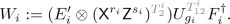
• 3. For all players h, $\mathsf {MPC}$ samples random ($4n+2$)-qubit Cliffords $D_{h}$, and gives them to the respective players. Starting with player i, each player h applies $D_{h}$ to $M^{ij}T^{ij}_{12}$,${}^\mathrm{a}$ and sends the state to player $h+1$. Eventually, player i receives the state back from player $i-1$. $\mathsf {MPC}$ remembers the applied Clifford

  $$ D := D_{i-1}D_{i-2} \cdots D_1 D_k D_{k-1} \cdots D_i. $$

• 4. $\mathsf {MPC}$ samples random ($2n+1$)-qubit Cliffords $F_i$ and $F_j$, and tells player i to apply

  $$ V := (F_i \otimes F_j) \mathsf {CNOT} _{1,2n+2}^{m_{\ell }} (E_i^{\dagger } \otimes \mathsf {I} ^{\otimes n} \otimes E_j^{\dagger } \otimes \mathsf {I} ^{\otimes n})D^{\dagger }. $$

  Here, the $\mathsf {CNOT}$ acts on the two data qubits inside the encodings.

• 5. If $i \ne j$, player i sends $M^jT^j_{12}$ to player j.

• 6. Players i and j publicly test their encodings. The procedures are identical, we describe the steps for player i:

  • (a) $\mathsf {MPC}$ samples a random $(n+1)$-qubit Clifford $E_i'$, which will be the new encoding key. Furthermore, $\mathsf {MPC}$ samples random n-bit strings $s_i$ and $r_i$, and a random classical invertible linear operator $g_i$ on $\mathbb {F}_2^{2n}$.

  • (b) $\mathsf {MPC}$ tells player i to apply

    

    Here, $U_{g_i}$ is as defined in Protocol 4.2.

  • (c) Player i measures $T_2^i$ in the computational basis and reports the n-bit measurement outcome $r_i'$ to the $\mathsf {MPC}$.

  • (d) $\mathsf {MPC}$ checks whether $r_i' = r_i$. If it is not, $\mathsf {MPC}$ sends abort to all players. If it is, the test has passed, and $\mathsf {MPC}$ stores the new encoding key $E_i'$ in its internal memory.

${}^\mathrm{a}$We combine subscripts and superscripts to denote multiple registers: e.g., $T^{ij}_{12}$ is shorthand for $T^i_1T^i_2T^j_1T^j_2$.

Lemma 5.5

Let $\varPi ^{\mathsf {CNOT} ^{m_\ell }}$ be Protocol 5.4, to be executed on wires $w_i$ and $w_j$, held by players i and j, respectively. Let $\mathfrak {I}^{C}$ be the ideal functionality for a circuit C as described in Definition 5.1. For all sets $I_{\mathcal {A}} \subsetneq [k]$ of corrupted players and all adversaries $\mathcal {A}$ that perform the interactions of players in $I_{\mathcal {A}}$, there exists a simulator $\mathcal {S}$ (the complexity of which scales polynomially in that of the adversary) such that for all environments $\mathcal {E}$,

$$ \left| \Pr [1 \leftarrow (\mathcal {E}\leftrightarrows (\varPi ^{\mathsf {CNOT} ^{m_\ell }} \diamond \mathfrak {I}^{C})_{\mathcal {A}})] = \Pr [1 \leftarrow (\mathcal {E}\leftrightarrows \mathfrak {I}^{\mathsf {CNOT} ^{m_\ell } \circ C}_{\mathcal {S}})]\right| \leqslant \mathsf {negl}\left( n\right) . $$

Proof

(sketch). There are four different cases, depending on which of players i and j are dishonest. In the full version, we provide a full proof by detailing the simulators for all four cases, but in this sketch, we only provide an intuition for the security in the case where both players are dishonest.

It is crucial that the adversary does not learn any information about the keys ($E_i, E_j, E'_i, E'_j$), nor about the randomizing elements ($r_i$, $r_j$, $s_i$, $s_j$, $g_i$, $g_j$). Even though the adversary learns $W_i, W_j$, and V explicitly during the protocol, all the secret information remains hidden by the randomizing Cliffords $F_i, F_j$, and D.

We consider a few ways in which the adversary may attack. First, he may prepare a non-zero state in the registers $T_2^{i}$ (or $T_2^{j}$) in step 2, potentially intending to spread those errors into $M^iT_1^i$ (or $M^jT_1^j$). Doing so, however, will cause $U_{g_i}$ (or $U_{g_j}$) to map the trap state to a random non-zero string, and the adversary would not know what measurement string $r_i'$ (or $r_j'$) to report. Since $g_i$ is unknown to the adversary, it suffices to measure $T^i_2$ in order to detect any errors in $T^i_{12}$.

Second, the adversary may fail to execute its instructions V or $W_i \otimes W_j$ correctly. Doing so is equivalent to attacking the state right before or right after these instructions. In both cases, however, the state in $M^iT_1^i$ is Clifford-encoded (and the state in $T_2^i$ is Pauli-encoded) with keys unknown to the adversary, so the authentication property of the Clifford code prevents the adversary from altering the outcome.

The simulator we define in the full version tests the adversary exactly for the types of attacks above. By using Pauli filters (see Definition 2.2), the simulator checks whether the attacker leaves the authenticated states and the trap states $T_2^i$ and $T_2^j$ (both at initialization and before measurement) unaltered. In the full proof, we show that the output state of the simulator approximates, up to an error negligible in n, the output state of the real protocol.

5.3 Subprotocol: Measurement

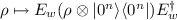
Measurement of authenticated states introduces a new conceptual challenge. For a random key E, the result of measuring in a fixed basis is in no way correlated with the logical measurement outcome of the state $\rho$. However, the measuring player is also not allowed to learn the key E, so they cannot perform a measurement in a basis that depends meaningfully on E.

In [DNS10, Appendix E], this challenge is solved by entangling the state with an ancilla-zero state on a logical level. After this entanglement step, Alice gets the original state while Bob gets the ancilla state. They both decode their state (learning the key from the $\mathsf {MPC}$), and can measure it. Because those states are entangled, and at least one of Alice and Bob is honest, they can ensure that the measurement outcome was not altered, simply by checking that they both obtained the same outcome. The same strategy can in principle also be scaled up to k players, by making all k players hold part of a big (logically) entangled state. However, doing so requires the application of $k-1$ logical $\mathsf {CNOT}$ operations, making it a relatively expensive procedure.

We take a different approach in our protocol. The player that performs the measurement essentially entangles, with the help of the $\mathsf {MPC}$, the data qubit with a random subset of the traps. The $\mathsf {MPC}$ later checks the consistency of the outcomes: all entangled qubits should yield the same measurement result.

Our alternative approach has the additional benefit that the measurement outcome can be kept secret from some or all of the players. In the description of the protocol below, the $\mathsf {MPC}$ stores the measurement outcome in its internal state. This allows the $\mathsf {MPC}$ to classically control future gates on the outcome. If it is desired to instead reveal the outcome to one or more of the players, this can easily be done by performing a classically-controlled $\mathsf {X}$ operation on some unused output qubit of those players.

Protocol 5.6 (Computational-basis measurement). Player i holds an encoding of the state in a wire w in the register $MT_1$. The classical $\mathsf {MPC}$ holds the encoding key E in the register S.

• 1. $\mathsf {MPC}$ samples random strings $r,s \in \{0,1\}^{n+1}$ and $c \in \{0,1\}^n$.

• 2. $\mathsf {MPC}$ tells player i to apply

  $$ V := \mathsf {X} ^r\mathsf {Z} ^s \mathsf {CNOT} _{1,c} E^{\dagger } $$

  to the register $MT_1$, where $\mathsf {CNOT} _{1,c}$ denotes the unitary $\prod _{i \in [n]} \mathsf {CNOT} _{1,i}^{c_i}$ (that is, the string c dictates with which of the qubits in $T_1$ the M register will be entangled).

• 3. Player i measures the register $MT_1$ in the computational basis, reporting the result $r'$ to $\mathsf {MPC}$.

• 4. $\mathsf {MPC}$ checks whether $r' = r \oplus (m, m\cdot c)$ for some $m \in \{0,1\}$.${}^\mathrm{a}$ If so, it stores the measurement outcome m in the state register S. Otherwise, it aborts by storing $\bot$ in S.

• 5. $\mathsf {MPC}$ removes the key E from the state register S.

${}^\mathrm{a}$The $\cdot$ symbol represents scalar multiplication of the bit m with the string c.

Lemma 5.7

Let C be a circuit on W wires that leaves some wire $w \leqslant W$ unmeasured. Let $\mathfrak {I}^{C}$ be the ideal functionality for C, as described in Definition 5.1, and let be Protocol 5.6 for a computational-basis measurement on w. For all sets $I_{\mathcal {A}} \subsetneq [k]$ of corrupted players and all adversaries $\mathcal {A}$ that perform the interactions of players in $I_{\mathcal {A}}$, there exists a simulator $\mathcal {S}$ (the complexity of which scales polynomially in that of the adversary) such that for all environments $\mathcal {E}$,

Proof

(sketch). The operation $\mathsf {CNOT} _{1,c}$ entangles the data qubit in register M with a random subset of the trap qubits in register $T_1$, as dictated by c. In step 4 of Protocol 5.6, the $\mathsf {MPC}$ checks both for consistency of all the bits entangled by c (they have to match the measured data) and all the bits that are not entangled by c (they have to remain zero).

In the full version, we show that checking the consistency of a measurement outcome after the application of $\mathsf {CNOT} _{1,c}$ is as good as measuring the logical state: any attacker that does not know c will have a hard time influencing the measurement outcome, as he will have to flip all qubits in positions i for which $c_i = 1$ without accidentally flipping any of the qubits in positions i for which $c_i = 0$. See the full version for a full proof that the output state in the real and simulated case are negligibly close.

5.4 Subprotocol: Decoding

After the players run the computation subprotocols for all gates in the Clifford circuit, all they need to do is to decode their wires to recover their output. At this point, there is no need to check the authentication traps publicly: there is nothing to gain for a dishonest player by incorrectly measuring or lying about their measurement outcome. Hence, it is sufficient for all (honest) players to apply the regular decoding procedure for the Clifford code.

Below, we describe the decoding procedure for a single wire held by one of the players. If there are multiple output wires, then Protocol 5.8 can be run in parallel for all those wires.

Protocol 5.8 (Decoding). Player i holds an encoding of the state w in the register $MT_1$. The classical $\mathsf {MPC}$ holds the encoding key E in the state register S.

• 1. $\mathsf {MPC}$ sends E to player i, removing it from the state register S.

• 2. Player i applies E to register $MT_1$.

• 3. Player i measures $T_1$ in the computational basis. If the outcome is not $0^n$, player i discards M and aborts the protocol.

Lemma 5.9

Let C be a circuit on W wires that leaves a single wire $w \leqslant W$ (intended for player i) unmeasured. Let $\mathfrak {I}^{C}$ be the ideal functionality for C, as described in Definition 5.1, and let $\mathfrak {I}^{\mathsf {MPQC}}_{C}$ be the ideal MPQC functionality for C, as described in Definition 3.1. Let $\varPi ^{\mathsf {Dec}}$ be Protocol 5.8 for decoding wire w. For all sets $I_{\mathcal {A}} \subsetneq [k]$ of corrupted players and all adversaries $\mathcal {A}$ that perform the interactions of players in $I_{\mathcal {A}}$, there exists a simulator $\mathcal {S}$ (the complexity of which scales polynomially in that of the adversary) such that for all environments $\mathcal {E}$,

$$ \Pr [1 \leftarrow (\mathcal {E}\leftrightarrows (\varPi ^{\mathsf {Dec}} \diamond \mathfrak {I}^{C})_{\mathcal {A}})] = \Pr [1 \leftarrow (\mathcal {E}\leftrightarrows \mathfrak {I}^{\mathsf {MPQC}}_{C,\mathcal {S}})]. $$

Proof

(sketch). If player i is honest, then he correctly decodes the state received from the ideal functionality $\mathfrak {I}^{C}$. A simulator would only have to compute the adversary’s abort bit for $\mathfrak {I}^{\mathsf {MPQC}}_{C}$ based on whether the adversary decides to abort in either $\mathfrak {I}^{C}$ or the $\mathsf {MPC}$ computation in $\varPi ^{\mathsf {Dec}}$.

If player i is dishonest, a simulator $\mathcal {S}$ runs the adversary on the input state received from the environment before inputting the resulting state into the ideal functionality $\mathfrak {I}^{\mathsf {MPQC}}_{C}$. The simulator then samples a key for the Clifford code and encodes the output of $\mathfrak {I}^{\mathsf {MPQC}}_C$, before handing it back to the adversary. It then simulates $\varPi ^{\mathsf {Dec}}$ by handing the sampled key to the adversary. If the adversary aborts in one of the two simulated protocols, then the simulator sends abort to the ideal functionality $\mathfrak {I}^{\mathsf {MPQC}}_C$.

5.5 Combining Subprotocols

We show in this section how to combine the subprotocols of the previous sections in order to perform multi-party quantum Clifford computation.

Recalling the notation defined in Definition 3.1, let C be a quantum circuit on $W \in \mathbb {N}_{>0}$ wires, which are partitioned into the players’ input registers plus an ancillary register, as $[W] = R_1^{\mathsf {in}} \sqcup \cdots \sqcup R_k^{\mathsf {in}} \sqcup R^{\mathsf {ancilla}}$, and a partition into the players’ output registers plus a register that is discarded at the end of the computation, as $[W] = R_1^{\mathsf {out}} \sqcup \cdots \sqcup R_k^{\mathsf {out}} \sqcup R^{\mathsf {discard}}$. We assume that C is decomposed in a sequence $G_1,...,G_m$ of operations where each $G_i$ is one of the following operations:

• a single-qubit Clifford on some wire $j \in [M]$;

• a CNOT on wires $j_1,j_2 \in [M]$ for $j_1 \ne j_2$;

• a measurement of the qubit on wire j in the computational basis.

In Sects. 4 and 5.1–5.3, we have presented subprotocols for encoding single qubits and perform these types of operations on single wires. The protocol for all players to jointly perform the bigger computation C is simply a concatenation of those smaller subprotocols:

Protocol 5.10 (Encoding and Clifford+measurement computation). Let C be a Clifford+measurement circuit composed of the gates $G_1, \dots , G_m$ on wires [W] as described above.

• 1. For all $i \in [k]$ and $j \in R^{\mathsf {in}}_i$, run Protocol 4.2 for the qubit in wire j.

• 2. For all $j \in R^{\mathsf {ancilla}}$, run Protocol 4.2 (with the differences described in Sect. 4.2).

• 3. For all $j \in [m]$:

  • (a) If $G_j$ is a single-qubit Clifford, run Protocol 5.2 for $G_j$.

  • (b) If $G_j$ is a CNOT, run Protocol 5.4 for $G_j$.

  • (c) If $G_j$ is a computational-basis measurement, run Protocol 5.6 for $G_j$.

• 4. For all $i \in [k]$ and $j \in R^{\mathsf {out}}_i$, run Protocol 5.8 for the qubit in wire j.

Lemma 5.11

Let $\varPi ^{\mathsf {Cliff}}$ be Protocol 5.10, and $\mathfrak {I}^{\mathsf {Cliff}}$ be the ideal functionality described in Definition 3.1 for the special case where the circuit consists of (a polynomial number of) Cliffords and measurements. For all sets $I_{\mathcal {A}} \subsetneq [k]$ of corrupted players and all adversaries $\mathcal {A}$ that perform the interactions of players in $I_{\mathcal {A}}$ with $\varPi$, there exists a simulator $\mathcal {S}$ (the complexity of which scales polynomially in that of the adversary) such that for all environments $\mathcal {E}$,

$$ |\Pr [1 \leftarrow (\mathcal {E}\leftrightarrows \varPi ^{\mathsf {Cliff}}_{\mathcal {A}})] - \Pr [1 \leftarrow (\mathcal {E}\leftrightarrows \mathfrak {I}^{\mathsf {Cliff}}_{\mathcal {S}})| \leqslant \mathsf {negl}\left( n\right) . $$

Proof

The proof by induction on m is given in the full version.

6 Protocol: MPQC for General Quantum Circuits

In this section, we show how to lift the MPQC for Clifford operations (as laid out in Sects. 4 and 5) to MPQC for general quantum circuits.

The main idea is to use magic states for $\mathsf {T}$ gates, as described in Sect. 2.5. Our main difficulty here is that the magic states must be supplied by the possibly dishonest players themselves. We solve this problem in Sect. 6.1 and then in Sect. 6.2, we describe the MPQC protocol for universal computation combining the results from Sects. 5 and 6.1.

6.1 Magic-State Distillation

We now describe a subprotocol that allows the players to create the encoding of exponentially good magic states, if the players do not abort.

Our subprotocol can be divided into two parts. In the first part, player 1 is asked to create many magic states, which the other players will test. After this step, if none of the players abort during the testing, then with high probability the resource states created by player 1 are at least somewhat good. In the second part of the subprotocol, the players run a distillation procedure to further increase the quality of the magic states.

Protocol 6.1 (Magic-state creation). Let t be the number of magic states we wish to create. Let $\ell := (t+k)n$.

• 1. Player 1 creates $\ell$ copies of $\left| \mathsf {T} \right\rangle$ and encodes them separately using Protocol 4.2 (jointly with the other players).

• 2. $\mathsf {MPC}$ picks random disjoint sets $S_2,\dots ,S_k \subseteq [\ell ]$ of size n each.

• 3. For each $i \in 2,\dots ,k$, player i decodes the magic states indicated by $S_i$ (see Protocol 5.8), measures in the $\{\left| \mathsf {T} \right\rangle , \left| \mathsf {T} ^\perp \right\rangle \}$-basis and aborts if any outcome is different from $\left| \mathsf {T} \right\rangle$.

• 4. On the remaining encoded states, the players run Protocol 5.10 for multi-party computation of Clifford circuits (but skipping the input-encoding step) to perform the magic-state distillation protocol described in Protocol 2.8. Any randomness required in that protocol is sampled by the classical $\mathsf {MPC}$.

We claim that Protocol 6.1 implements the following ideal functionality for creating t magic states, up to a negligible error:

Definition 6.2

(Ideal functionality for magic-state creation). Let t be the number of magic states we wish to create. Let $I_{\mathcal {A}} \subsetneq [k]$ be a set of corrupted players.

• 1. For every $i \in I_{\mathcal {A}}$, player i sends a bit $b_{i}$ to the trusted third party.

  • (a) If $b_{i} = 0$ for all i, the trusted third party samples t random $(n+1)$-qubit Clifford $E_j$ for $1 \leqslant j \leqslant t$, and sends $E_j(\left| \mathsf {T}\right\rangle \otimes \left| 0^n\right\rangle )$ to Player 1.

  • (b) Otherwise, the trusted third party sends abort to all players.

• 2. Store the keys $E_j$, for $1 \leqslant j \leqslant t$ in the state register S of the ideal functionality.

Lemma 6.3

Let $\varPi ^{MS}$ be Protocol 6.1, and $\mathfrak {I}^{MS}$ be the ideal functionality described in Definition 6.2. For all sets $I_{\mathcal {A}} \subsetneq [k]$ of corrupted players and all adversaries $\mathcal {A}$ that perform the interactions of players in $I_{\mathcal {A}}$ with $\varPi$, there exists a simulator $\mathcal {S}$ (the complexity of which scales polynomially in that of the adversary) such that for all environments $\mathcal {E}$,

$$ \left| \Pr [1 \leftarrow (\mathcal {E}\leftrightarrows \varPi ^{MS}_{\mathcal {A}})] - \Pr [1 \leftarrow (\mathcal {E}\leftrightarrows \mathfrak {I}^{MS}_{\mathcal {S}})\right| \leqslant \mathsf {negl}\left( n\right) .$$

We prove this lemma in the full version.

6.2 MPQC Protocol for Universal Quantum Computation

Finally, we present our protocol for some arbitrary quantum computation. For this setting, we extend the setup of Sect. 5.5 by considering quantum circuits $C = G_m...G_1$ where $G_i$ can be single-qubit Cliffords, CNOTs, measurements or, additionally, $\mathsf {T}$ gates.

For that, we will consider a circuit $C'$ where each gate $G_i = \mathsf {T}$ acting on qubit j is then replaced by the $\mathsf {T}$-gadget presented in Fig. 1, acting on the qubit j and a fresh new $\mathsf {T}$ magic state.

Protocol 6.4 (Protocol for universal MPQC). Let C be a polynomial-sized quantum circuit, and t be the number of $\mathsf {T}$-gates in C.

• 1. Run Protocol 6.1 to create t magic states.

• 2. Run Protocol 5.10 for the circuit $C'$, which is equal to the circuit C, except each $\mathsf {T}$ gate is replaced with the $\mathsf {T}$-gadget from Fig. 1.

Theorem 6.5

Let $\varPi ^{\mathsf {MPQC}}$ be Protocol 6.4, and $\mathfrak {I}^{\mathsf {MPQC}}$ be the ideal functionality described in Definition 3.1. For all sets $I_{\mathcal {A}} \subsetneq [k]$ of corrupted players and all adversaries $\mathcal {A}$ that perform the interactions of players in $I_{\mathcal {A}}$ with $\varPi$, there exists a simulator $\mathcal {S}$ (the complexity of which scales polynomially in that of the adversary) such that for all environments $\mathcal {E}$,

$$ |\Pr [1 \leftarrow (\mathcal {E}\leftrightarrows \varPi ^{\mathsf {MPQC}}_{\mathcal {A}})] - \Pr [1 \leftarrow (\mathcal {E}\leftrightarrows \mathfrak {I}^{\mathsf {MPQC}}_{\mathcal {S}})| \leqslant \mathsf {negl}\left( n\right) . $$

Proof

Direct from Lemmas 5.11 and 6.3.

6.3 Round Complexity and MPC Calls

Recall that we are assuming access to an ideal (classical) MPC functionality defined in Definition 2.1. One MPC call can produce outputs to all players simultaneously. In this section, we analyze the number of rounds of quantum communication, and the number of calls to the classical MPC. The actual implementation of the classical MPC is likely to result in additional rounds of classical communication.

In the way we describe it, Lemma 4.2 encodes a single-qubit input (or an ancilla $\left| 0\right\rangle$ state) using k rounds of quantum communication and O(1) MPC calls. Note that this protocol can be run in parallel for all input qubits per player, simultaneously for all players. Hence, the overall number of communication rounds for the encoding phase remains k, and the total number of calls to the MPC is O(w) where w is the total number of qubits.

Lemma 5.2 for single-qubit Cliffords, Lemma 5.6 for measuring in the computational basis and Lemma 5.8 for decoding do not require quantum communication and use O(1) MPC calls each, whereas Lemma 5.4 for $\mathsf {CNOT}$ requires at most $k+2$ rounds of quantum communication, and makes O(1) MPC calls. Overall, Lemma 5.10 for encoding and Clifford+measurement computation require O(dk) rounds of quantum communication and $O(w + g)$ calls to the MPC, where d is the $\mathsf {CNOT}$-depth of the quantum circuit, and g is the total number of gates in the circuit.

Lemma 6.1 for magic-state creation encodes $\ell := (t+k)n$ qubits in parallel using k rounds of quantum communication (which can be done in parallel with the actual input encoding) and $O((t+k)n)$ MPC calls. Then a circuit of size $p_{\mathrm {distill}}(n)$ and $\mathsf {CNOT}$-depth $d_{\mathrm {distill}}(n)$ classically controlled Cliffords and measurements is run on each of the t blocks of n qubits each, which can be done in parallel for the t blocks, requiring $O(k \cdot d_{\mathrm {distill}}(n))$ rounds of quantum communication and $O(tn\cdot p_{\mathrm {distill}}(n))$ calls to the MPC.

Eventually, all $\mathsf {T}$-gate operations in the original circuit C are replaced by the $\mathsf {T}$-gadget from Fig. 1, resulting in one $\mathsf {CNOT}$ and classically controlled Cliffords. Overall, our Lemma 6.4 for universal MPQC requires $O(k \cdot (d_{\mathrm {distill}}(n) + d))$ rounds of quantum communication and $O(tn\cdot p_{\mathrm {distill}}(n) + w + g)$ calls to the classical MPC, where d is the $\{\mathsf {CNOT}, \mathsf {T} \}$-depth of the circuit, w is the total number of qubits and g is the total number of gates in the circuit.

We notice that instead of evaluating each Clifford operation gate-by-gate, we could evaluate a general w-qubit Clifford using O(k) rounds of quantum communication, similarly to the $\mathsf {CNOT}$ protocol. This could improve the parameter d to be the $\mathsf {T}$ depth of the circuit, at the cost of requiring significantly more communication per round.

References

Aharonov, D., Ben-Or, M., Eban, E.: Interactive proofs for quantum computations. In: ICS 2010 (2010)
Bendlin, R., Damgård, I., Orlandi, C., Zakarias, S.: Semi-homomorphic encryption and multiparty computation. In: Paterson, K.G. (ed.) EUROCRYPT 2011. LNCS, vol. 6632, pp. 169–188. Springer, Heidelberg (2011). https://doi.org/10.1007/978-3-642-20465-4_11
Bravyi, S., Kitaev, A.: Universal quantum computation with ideal Clifford gates and noisy ancillas. Phys. Rev. A 71, 022316 (2005)
Ben-Or, M., Crépeau, C., Gottesman, D., Hassidim, A., Smith, A.: Secure multiparty quantum computation with (only) a strict honest majority. In: FOCS 2006 (2006)
Broadbent, A., Wainewright, E.: Efficient simulation for quantum message authentication. In: Nascimento, A.C.A., Barreto, P. (eds.) ICITS 2016. LNCS, vol. 10015, pp. 72–91. Springer, Cham (2016). https://doi.org/10.1007/978-3-319-49175-2_4
Cramer, R., Damgård, I., Escudero, D., Scholl, P., Xing, C.: SPD\(\mathbb{Z}_{2^k}\): efficient MPC mod \(2^k\) for dishonest majority. In: Shacham, H., Boldyreva, A. (eds.) CRYPTO 2018. LNCS, vol. 10992, pp. 769–798. Springer, Cham (2018). https://doi.org/10.1007/978-3-319-96881-0_26
Chase, M., et al.: Post-quantum zero-knowledge and signatures from symmetric-key primitives. In: CCS 2017 (2017)
Cramer, R., Damgård, I., Nielsen, J.B.: Secure Multiparty Computation and Secret Sharing. Cambridge University Press, Cambridge (2015)
Crépeau, C., Gottesman, D., Smith, A.: Secure multi-party quantum computation. In: STOC 2002 (2002)
Dupuis, F., Nielsen, J.B., Salvail, L.: Secure two-party quantum evaluation of unitaries against specious adversaries. In: Rabin, T. (ed.) CRYPTO 2010. LNCS, vol. 6223, pp. 685–706. Springer, Heidelberg (2010). https://doi.org/10.1007/978-3-642-14623-7_37
Dupuis, F., Nielsen, J.B., Salvail, L.: Actively secure two-party evaluation of any quantum operation. In: Safavi-Naini, R., Canetti, R. (eds.) CRYPTO 2012. LNCS, vol. 7417, pp. 794–811. Springer, Heidelberg (2012). https://doi.org/10.1007/978-3-642-32009-5_46
Damgård, I., Pastro, V., Smart, N., Zakarias, S.: Multiparty computation from somewhat homomorphic encryption. In: Safavi-Naini, R., Canetti, R. (eds.) CRYPTO 2012. LNCS, vol. 7417, pp. 643–662. Springer, Heidelberg (2012). https://doi.org/10.1007/978-3-642-32009-5_38
Ishai, Y., Kushilevitz, E., Ostrovsky, R., Sahai, A.: Zero-knowledge proofs from secure multiparty computation. SIAM J. Comput. 39(3), 1121–1152 (2009)
Kashefi, E., Music, L., Wallden, P.: The quantum cut-and-choose technique and quantum two-party computation. arXiv preprint arXiv:1703.03754 (2017)
Keller, M., Orsini, E., Scholl, P.: MASCOT: faster malicious arithmetic secure computation with oblivious transfer. In: CCS 2016 (2016)
Kashefi, E., Pappa, A.: Multiparty delegated quantum computing. Cryptography 1(2), 12 (2017)
Keller, M., Pastro, V., Rotaru, D.: Overdrive: making SPDZ great again. In: Nielsen, J.B., Rijmen, V. (eds.) EUROCRYPT 2018. LNCS, vol. 10822, pp. 158–189. Springer, Cham (2018). https://doi.org/10.1007/978-3-319-78372-7_6
Yao, A.C.-C.: Protocols for secure computations (extended abstract). In: FOCS 1982 (1982)
Acknowledgments
We thank Frédéric Dupuis, Florian Speelman, and Serge Fehr for useful discussions, and the anonymous EUROCRYPT referees for helpful comments and suggestions. CM is supported by an NWO Veni Innovational Research Grant under project number VI.Veni.192.159. SJ is supported by an NWO WISE Fellowship, an NWO Veni Innovational Research Grant under project number 639.021.752, and QuantERA project QuantAlgo 680-91-03. SJ is a CIFAR Fellow in the Quantum Information Science Program. CS and CM were supported by a NWO VIDI grant (Project No. 639.022.519). Part of this work was done while YD, AG and CS were visiting the Simons Institute for the Theory of Computing.
Author information
Authors and Affiliations
Corresponding authors
Editor information
Editors and Affiliations
Rights and permissions
Copyright information
© 2020 International Association for Cryptologic Research
About this paper
Cite this paper
Dulek, Y., Grilo, A.B., Jeffery, S., Majenz, C., Schaffner, C. (2020). Secure Multi-party Quantum Computation with a Dishonest Majority. In: Canteaut, A., Ishai, Y. (eds) Advances in Cryptology – EUROCRYPT 2020. EUROCRYPT 2020. Lecture Notes in Computer Science(), vol 12107. Springer, Cham. https://doi.org/10.1007/978-3-030-45727-3_25
Download citation
DOI: https://doi.org/10.1007/978-3-030-45727-3_25
Published:
Publisher Name: Springer, Cham
Print ISBN: 978-3-030-45726-6
Online ISBN: 978-3-030-45727-3
eBook Packages: Computer ScienceComputer Science (R0)