Constraint-Based Monitoring of Hyperproperties

Abstract

Verifying hyperproperties at runtime is a challenging problem as hyperproperties, such as non-interference and observational determinism, relate multiple computation traces with each other. It is necessary to store previously seen traces, because every new incoming trace needs to be compatible with every run of the system observed so far. Furthermore, the new incoming trace poses requirements on future traces. In our monitoring approach, we focus on those requirements by rewriting a hyperproperty in the temporal logic HyperLTL to a Boolean constraint system. A hyperproperty is then violated by multiple runs of the system if the constraint system becomes unsatisfiable. We compare our implementation, which utilizes either BDDs or a SAT solver to store and evaluate constraints, to the automata-based monitoring tool RVHyper.

This work was partially supported by the German Research Foundation (DFG) as part of the Collaborative Research Center “Methods and Tools for Understanding and Controlling Privacy” (CRC 1223) and the Collaborative Research Center “Foundations of Perspicuous Software Systems” (CRC 248), and by the European Research Council (ERC) Grant OSARES (No. 683300).

1 Introduction

As today’s complex and large-scale systems are usually far beyond the scope of classic verification techniques like model checking or theorem proving, we are in the need of light-weight monitors for controlling the flow of information. By instrumenting efficient monitoring techniques in such systems that operate in an unpredictable privacy-critical environment, countermeasures will be enacted before irreparable information leaks happen. Information-flow policies, however, cannot be monitored with standard runtime verification techniques as they relate multiple runs of a system. For example, observational determinism [19, 21, 24] is a policy stating that altering non-observable input has no impact on the observable behavior. Hyperproperties [7] are a generalization of trace properties and are thus capable of expressing information-flow policies. HyperLTL [6] is a recently introduced temporal logic for hyperproperties, which extends Linear-time Temporal Logic (LTL) [20] with trace variables and explicit trace quantification. Observational determinism is expressed as the formula , stating that all traces $\pi ,\pi '$ should agree on the output as long as they agree on the inputs.

In contrast to classic trace property monitoring, where a single run suffices to determine a violation, in runtime verification of HyperLTL formulas, we are concerned whether a set of runs through a system violates a given specification. In the common setting, those runs are given sequentially to the runtime monitor [1, 2, 12, 13], which determines if the given set of runs violates the specification. An alternative view on HyperLTL monitoring is that every new incoming trace poses requirements on future traces. For example, the event $\{ in , out \}$ in the observational determinism example above asserts that for every other trace, the output $out$ has to be enabled if $in$ is enabled. Approaches based on static automata constructions [1, 12, 13] perform very well on this type of specifications, although their scalability is intrinsically limited by certain parameters: The automaton construction becomes a bottleneck for more complex specifications, especially with respect to the number of atomic propositions. Furthermore, the computational workload grows steadily with the number of incoming traces, as every trace seen so far has to be checked against every new trace. Even optimizations [12], which minimize the amount of traces that must be stored, turn out to be too coarse grained as the following example shows. Consider the monitoring of the HyperLTL formula , which states that globally if a occurs on any trace $\pi$, then b is not allowed to hold on any trace $\pi '$, on the following incoming traces:

(1)

(2)

(3)

In prior work [12], we observed that traces, which pose less requirements on future traces, can safely be discarded from the monitoring process. In the example above, the requirements of trace 1 are dominated by the requirements of trace 2, namely that b is not allowed to hold on the first and second position of new incoming traces. Hence, trace 1 must not longer be stored in order to detect a violation. But with the proposed language inclusion check in [12], neither trace 2 nor trace 3 can be discarded, as they pose incomparable requirements. They have, however, overlapping constraints, that is, they both enforce $\lnot b$ in the first step.

To further improve the conciseness of the stored traces information, we use rewriting, which is a more fine-grained monitoring approach. The basic idea is to track the requirements that future traces have to fulfill, instead of storing a set of traces. In the example above, we would track the requirement that b is not allowed to hold on the first three positions of every freshly incoming trace. Rewriting has been applied successfully to trace properties, namely LTL formulas [17]. The idea is to partially evaluate a given LTL specification $\varphi$ on an incoming event by unrolling $\varphi$ according to the expansion laws of the temporal operators. The result of a single rewrite is again an LTL formula representing the updated specification, which the continuing execution has to satisfy. We use rewriting techniques to reduce $\forall ^2$HyperLTL formulas to LTL constraints and check those constraints for inconsistencies corresponding to violations.

In this paper, we introduce a complete and provably correct rewriting-based monitoring approach for $\forall ^2$HyperLTL formulas. Our algorithm rewrites a HyperLTL formula and a single event into a constraint composed of plain LTL and HyperLTL. For example, assume the event $\{ in , out \}$ while monitoring observational determinism formalized above. The first step of the rewriting applies the expansion laws for the temporal operators, which results in . The event $\{in, out\}$ is rewritten for atomic propositions indexed by the trace variable $\pi$. This means replacing each occurrence of in or out in the current expansion step, i.e., before the operator, with $\top$. Additionally, we strip the $\pi '$ trace quantifier in the current expansion step from all other atomic propositions. This leaves us with . After simplification we have as the new specification, which consists of a plain LTL part and a HyperLTL part. Based on this, we incrementally build a Boolean constraint system: we start by encoding the constraints corresponding to the LTL part and encode the HyperLTL part as variables. Those variables will then be incrementally defined when more elements of the trace become available. With this approach, we solely store the necessary information needed to detect violations of a given hyperproperty.

We evaluate two implementations of our approach, based on BDDs and SAT-solving, against RVHyper [13], a highly optimized automaton-based monitoring tool for temporal hyperproperties. Our experiments show that the rewriting approach performs equally well in general and better on a class of formulas which we call guarded invariants, i.e., formulas that define a certain invariant relation between two traces.

Related Work. With the need to express temporal hyperproperties in a succinct and formal manner, the above mentioned temporal logics HyperLTL and HyperCTL* [6] have been proposed. The model-checking [6, 14, 15], satisfiability [9], and realizability problem [10] of $\text {HyperLTL}~$ has been studied before.

Runtime verification of HyperLTL formulas was first considered for (co-)k-safety hyperproperties [1]. In the same paper, the notion of monitorability for HyperLTL was introduced. The authors have also identified syntactic classes of HyperLTL formulas that are monitorable and they proposed a monitoring algorithm based on a progression logic expressing trace interdependencies and the composition of an LTL$_3$ monitor.

Another automata-based approach for monitoring HyperLTL formulas was proposed in [12]. Given a HyperLTL specification, the algorithm starts by creating a deterministic monitor automaton. For every incoming trace it is then checked that all combinations with the already seen traces are accepted by the automaton. In order to minimize the number of stored traces, a language-inclusion-based algorithm is proposed, which allows to prune traces with redundant information. Furthermore, a method to reduce the number of combination of traces which have to get checked by analyzing the specification for relations such as reflexivity, symmetry, and transitivity with a HyperLTL-SAT solver [9, 11], is proposed. The algorithm is implemented in the tool RVHyper [13], which was used to monitor information-flow policies and to detect spurious dependencies in hardware designs.

Another rewriting-based monitoring approach for HyperLTL is outlined in [5]. The idea is to identify a set of propositions of interest and aggregate constraints such that inconsistencies in the constraints indicate a violation of the HyperLTL formula. While the paper describes the building blocks for such a monitoring approach with a number of examples, we have, unfortunately, not been successful in applying the algorithm to other hyperproperties of interest, such as observational determinism.

In [3], the authors study the complexity of monitoring hyperproperties. They show that the form and size of the input, as well as the formula have a significant impact on the feasibility of the monitoring process. They differentiate between several input forms and study their complexity: a set of linear traces, tree-shaped Kripke structures, and acyclic Kripke structures. For acyclic structures and alternation-free HyperLTL formulas, the problems complexity gets as low as NC.

In [4], the authors discuss examples where static analysis can be combined with runtime verification techniques to monitor HyperLTL formulas beyond the alternation-free fragment. They discuss the challenges in monitoring formulas beyond this fragment and lay the foundations towards a general method.

2 Preliminaries

Let $AP$ be a finite set of atomic propositions and let $\varSigma = 2^ AP$ be the corresponding alphabet. An infinite trace $t \in \varSigma ^\omega$ is an infinite sequence over the alphabet. A subset $T \subseteq \varSigma ^\omega$ is called a trace property. A hyperproperty $H \subseteq 2^{(\varSigma ^\omega )}$ is a generalization of a trace property. A finite trace $t \in \varSigma ^+$ is a finite sequence over $\varSigma$. In the case of finite traces, |t| denotes the length of a trace. We use the following notation to access and manipulate traces: Let t be a trace and i be a natural number. t[i] denotes the i-th element of t. Therefore, t[0] represents the first element of the trace. Let j be natural number. If $j \ge i$ and $i\ge |t|$, then t[i, j] denotes the sequence $t[i] t[i+1] \cdots t[min(j,|t|-1)]$. Otherwise it denotes the empty trace $\epsilon$. $t[i\rangle$ denotes the suffix of t starting at position i. For two finite traces s and t, we denote their concatenation by $s \cdot t$.

HyperLTL Syntax. HyperLTL [6] extends LTL with trace variables and trace quantifiers. Let $\mathcal {V}$ be a finite set of trace variables. The syntax of HyperLTL is given by the grammar

where $a \in AP$ is an atomic proposition and $\pi \in \mathcal {V}$ is a trace variable. Atomic propositions are indexed by trace variables. The explicit trace quantification enables us to express properties like “on all traces $\varphi$ must hold”, expressed by $\forall \pi \mathpunct {.}\varphi$. Dually, we can express “there exists a trace such that $\varphi$ holds”, expressed by $\exists \pi \mathpunct {.}\varphi$. We use the standard derived operators release , eventually , globally , and weak until . As we use the finite trace semantics, denotes the strong version of the next operator, i.e., if a trace ends before the satisfaction of $\varphi$ can be determined, the satisfaction relation, defined below, evaluates to false. To enable duality in the finite trace setting, we additionally use the weak next operator which evaluates to true if a trace ends before the satisfaction of $\varphi$ can be determined and is defined as . We call $\psi$ of a HyperLTL formula ${\varvec{Q}}. \psi$, with an arbitrary quantifier prefix ${\varvec{Q}}$, the body of the formula. A HyperLTL formula ${\varvec{Q}}. \psi$ is in the alternation-free fragment if either ${\varvec{Q}}$ consists solely of universal quantifiers or solely of existential quantifiers. We also denote the respective alternation-free fragments as the $\forall ^n$ fragment and the $\exists ^n$ fragment, with n being the number of quantifiers in the prefix.

Finite Trace Semantics. We recap the finite trace semantics for HyperLTL [5] which is itself based on the finite trace semantics of $\text {LTL}$ [18]. In the following, when using $\mathcal {L}(\varphi )$ we refer to the finite trace semantics of a HyperLTL formula $\varphi$. Let $\varPi _ fin : \mathcal {V}\rightarrow \varSigma ^+$ be a partial function mapping trace variables to finite traces. We define $\epsilon [0]$ as the empty set. denotes the trace assignment that is equal to for all . By slight abuse of notation, we write to access traces t in the image of . The satisfaction of a HyperLTL formula $\varphi$ over a finite trace assignment and a set of finite traces T, denoted by , is defined as follows:

Due to duality of , , $\exists$/$\forall$, and the standard Boolean operators, every HyperLTL formula $\varphi$ can be transformed into negation normal form (NNF), i.e., for every $\varphi$ there is some $\psi$ in negation normal form such that for all and T it holds that if, and only if, . The standard LTL semantic, written , for some LTL formula $\varphi$ is equal to , where $\varphi '$ is derived from $\varphi$ by replacing every proposition $p \in AP$ by $p_\pi$.

3 Rewriting HyperLTL

Given the body $\varphi$ of a $\forall ^2$HyperLTL formula $\forall \pi ,\pi ' \mathpunct {.}\varphi$, and a finite trace $t \in \varSigma ^+$, we define alternative language characterizations. These capture the intuitive idea that, if one fixes a finite trace t, the language of $\forall \pi ,\pi ' \mathpunct {.}\varphi$ includes exactly those traces $t'$ that satisfy $\varphi$ in conjunction with t.

We call the symmetric closure of $\varphi$, where $\varphi [\pi '/\pi , \pi /\pi ']$ represents the expression $\varphi$ in which the trace variables $\pi , \pi '$ are swapped. The language of the symmetric closure, when fixing one trace variable, is equivalent to the language of $\varphi$.

Lemma 1

Given the body $\varphi$ of a $\forall ^2$HyperLTL formula $\forall \pi ,\pi ' \mathpunct {.}\varphi$, and a finite trace $t \in \varSigma ^+$, it holds that $\mathcal {L}^{\pi }_{t}(\hat{\varphi }) = \mathcal {L}_{t}(\varphi )$.

Proof

We exploit this to rewrite a $\forall ^2$HyperLTL formula into an LTL formula. We define the projection $\varphi |^{\pi }_{t}$ of the body $\varphi$ of a $\forall ^2$HyperLTL formula $\forall \pi ,\pi ' \mathpunct {.}\varphi$ in NNF and a finite trace $t \in \varSigma ^+$ to an $\text {LTL}$ formula recursively on the structure of $\varphi$:

Theorem 1

Given a $\forall ^2$HyperLTL formula $\forall \pi , \pi ' \mathpunct {.}\varphi$ and any two finite traces $t,t' \in \varSigma ^+$ it holds that .

Proof

By induction on the size of t. Induction Base ($t=e$, where $e \in \varSigma$): Let $t' \in \varSigma ^+$ be arbitrarily chosen. We distinguish by structural induction the following cases over the formula $\varphi$. We begin with the base cases.

• $a_{\pi }$: we know by definition that $a_{\pi }|^{\pi }_{t}$ equals $\top$ if $a \in t[0]$ and $\bot$ otherwise, so it follows that .

• $a_{\pi '}$: .

• $\lnot a_{\pi }$ and $\lnot a_{\pi '}$ are proven analogously.

The structural induction hypothesis states that (SIH1), where $\psi$ is a strict subformula of $\varphi$.

• 

• .

• 

• are proven analogously.

Induction Step ($t = e \cdot t^*$, where $e \in \varSigma , t^* \in \varSigma ^+$): The induction hypothesis states that (IH). We make use of structural induction over $\varphi$. All cases without temporal operators are covered as their proofs above were independent of |t|. The structural induction hypothesis states for all strict subformulas $\psi$ that (SIH2).

• 
• 

• are proven analogously.

4 Constraint-Based Monitoring

For monitoring, we need to define an incremental rewriting that accurately models the semantics of $\varphi |^{\pi }_{t}$ while still being able to detect violations early. To this end, we define an operation $\varphi [\pi ,e,i]$, where $e \in \varSigma$ is an event and i is the current position in the trace. $\varphi [\pi ,e,i]$ transforms $\varphi$ into a propositional formula, where the variables are either indexed atomic propositions $p_i$ for $p \in AP$, or a variable $v^{-}_{\varphi ',i+1}$ and $v^{+}_{\varphi ',i+1}$ that act as placeholders until new information about the trace comes in. Whenever the next event $e'$ occurs, the variables are defined with the result of $\varphi '[\pi ,e',i\,+\,1]$. If the trace ends, the variables are set to true and false for $v^{+}$ and $v^{-}$, respectively. We define $\varphi [\pi ,e,i]$ of a $\forall ^2$HyperLTL formula $\forall \pi ,\pi ' \mathpunct {.}\varphi$ in NNF, event $e \in \varSigma$, and $i \ge 0$ recursively on the structure of the body $\varphi$:

We encode a $\forall ^2$HyperLTL formula and finite traces into a constraint system, which, as we will show, is satisfiable if and only if the given traces satisfy the formula w.r.t. the finite semantics of HyperLTL. We write $v_{\varphi ,i}$ to denote either $v^{-}_{\varphi ,i}$ or $v^{+}_{\varphi ,i}$. For $e \in \varSigma$ and $t \in \varSigma ^*$, we define

where we use $v_{\psi ,i+1} \in \varphi [\pi , e, i]$ to denote variables $v_{\psi ,i+1}$ occurring in the propositional formula $\varphi [\pi , e, i]$. $enc$ is used to transform a trace into a propositional formula, e.g., $enc^{0}_{\{a,b\}}(\{a\}\{a,b\}) = a_0\,\wedge \,\lnot b_0\,\wedge \,a_1\,\wedge \,b_1$. For $n=0$ we omit the annotation, i.e., we write $enc_{\text {AP}}(t)$ instead of $enc^{0}_{\text {AP}}(t)$. Also we omit the index $\text {AP}$ if it is clear from the context. By slight abuse of notation, we use $constr^{n}(\varphi ,t)$ for some quantifier free HyperLTL formula $\varphi$ to denote $constr(v_{\varphi ,n},t)$ if ${|t|} > 0$. For a trace $t' \in \varSigma ^+$, we use the notation $enc(t') \vDash constr(\varphi ,t),$ which evaluates to true if, and only if $enc(t') \wedge constr(\varphi ,t)$ is satisfiable.

4.1 Algorithm

Figure 1 depicts our constraint-based algorithm. Note that this algorithm can be used in an offline and online fashion. Before we give algorithmic details, consider again, the observational determinism example from the introduction, which is expressed as $\forall ^2$HyperLTL formula . The basic idea of the algorithm is to transform the HyperLTL formula to a formula consisting partially of LTL, which expresses the requirements of the incoming trace in the current step, and partially of HyperLTL. Assuming the event $\{in,out\}$, we transform the observational determinism formula to the following formula: .

Fig. 1.

Constraint-based algorithm for monitoring $\forall ^2\text {HyperLTL}~$ formulas.

A Boolean constraint system is then build incrementally: we start encoding the constraints corresponding to the LTL part (in front of the next-operator) and encode the HyperLTL part (after the next-operator) as variables that are defined when more events of the trace come in. We continue by explaining the algorithm in detail. In line 1, we construct $\psi$ as the negation normal form of the symmetric closure of the original formula. We build two constraint systems: C containing constraints of previous traces and $C_t$ (built incrementally) containing the constraints for the current trace t. Consequently, we initialize C with $\top$ and $C_t$ with $v_{\psi ,0}$ (lines 2 and 4). If the trace ends, we define the remaining $v$ variables according to their polarities and add $C_t$ to C. For each new event $e_i$ in the trace t, and each “open” constraint in $C_t$ corresponding to step i, i.e., $v_{\phi ,i} \in C_t$, we rewrite the formula $\phi$ (line 9) and define $v_{\phi ,i}$ with the rewriting result, which, potentially introduced new open constraints $v_{\phi ',i+1}$ for the next step $i+1$. The constraint encoding of the current trace is aggregated in constraint $t_ enc$ (line 7). If the constraint system given the encoding of the current trace turns out to be unsatisfiable, a violation to the specification is detected, which is then returned.

In the following, we sketch two algorithmic improvements. First, instead of storing the constraints corresponding to traces individually, we use a new data structure, which is a tree maintaining nodes of formulas, their corresponding variables and also child nodes. Such a node corresponds to already seen rewrites. The initial node captures the (transformed) specification (similar to line 4) and it is also the root of the tree structure, representing all the generated constraints which replaces C in Fig. 1. Whenever a trace deviates in its rewrite result a new child or branch is added to the tree. If a rewrite result is already present in the node tree structure there is no need to create any new constraints nor new variables. This is crucial in case we observe many equal traces or traces behaving effectively the same. In case no new constraints were added to the constraint system, we omit a superfluous check for satisfiability.

Second, we use conjunct splitting to utilize the node tree optimization even more. We illustrate the basic idea on an example. Consider $\forall \pi , \pi ' \mathpunct {.}\varphi$ with , which demands that on all executions on each position at least on of propositions a or b agree in its evaluation. Consider the two traces $t_1 = \{a\}\{a\}\{a\}$, $t_2 = \{a\}\{a,b\}\{a\}$ that satisfy the specification. As both traces feature the same first event, they also share the same rewrite result for the first position. Interestingly, on the second position, we get $(a \vee \lnot b) \wedge s_\varphi$ for $t_1$ and $(a \vee b) \wedge s_\varphi$ for $t_2$ as the rewrite results. While these constraints are no longer equal, by the nature of invariants, both feature the same subterm on the right hand side of the conjunction. We split the resulting constraint on its syntactic structure, such that we would no longer have to introduce a branch in the tree.

4.2 Correctness

In this technical subsection, we will formally prove correctness of our algorithm by showing that our incremental construction of the Boolean constraints is equisatisfiable to the HyperLTL rewriting presented in Sect. 3. We begin by showing that satisfiability is preserved when shifting the indices, as stated by the following lemma.

Lemma 2

For any $\forall ^2$HyperLTL formula $\forall \pi ,\pi ' \mathpunct {.}\varphi$ over atomic propositions $\text {AP}$, any finite traces $t,t' \in \varSigma ^+$ and $n \ge 0$ it holds that $enc_{\text {AP}}(t') \vDash constr(\varphi ,t) \Leftrightarrow enc^{n}_{\text {AP}}(t') \vDash constr^{n}(\varphi ,t)$.

Proof

By renaming of the positional indices.

In the following lemma and corollary, we show that the semantics of the next operators matches the finite LTL semantics.

Lemma 3

For any $\forall ^2$HyperLTL formula $\forall \pi ,\pi ' \mathpunct {.}\varphi$ over atomic propositions $\text {AP}$ and any finite traces $t,t' \in \varSigma ^+$ it holds that

Proof

Let $\varphi$, $t,t'$ be given. It holds that by definition. As $constr(v^{-}_{\varphi ,1},t[1\rangle )$ by construction does not contain any variables with positional index 0, we only need to check satisfiability with respect to $enc(t'[1\rangle )$. Thus .

Corollary 1

For any $\forall ^2$HyperLTL formula $\forall \pi ,\pi ' \mathpunct {.}\varphi$ over atomic propositions $\text {AP}$ and any finite traces $t,t' \in \varSigma ^+$ it holds that

We will now state the correctness theorem, namely that our algorithm preserves the HyperLTL rewriting semantics.

Theorem 2

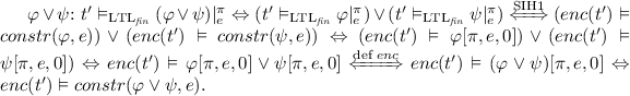
For every $\forall ^2$HyperLTL formula $\forall \pi ,\pi ' \mathpunct {.}\varphi$ in negation normal form over atomic propositions $\text {AP}$ and any finite trace $t \in \varSigma ^+$ it holds that .

Proof

By induction over the size of t. Induction Base ($t = e$, where $e \in \varSigma$): We choose $t' \in \varSigma ^+$ arbitrarily. We distinguish by structural induction the following cases over the formula $\varphi$:

• $a_{\pi }$: $constr(a_{\pi },e) = (a_\pi )[\pi ,e,0] = \top \text { if, and only if, } a \in e$. Thus .

• $a_{\pi '}$: $constr(a_{\pi '},e) = (a_{\pi '})[\pi ,e,0] = a_0$ Thus .

• $\lnot a_{\pi }$ and $\lnot a_{\pi '}$ are proven analogously.

The structural induction hypothesis states that (SIH1), where $\psi$ is a strict subformula of $\varphi$.

• 

• . Thus

• . Thus

• $\varphi \wedge \psi$, are proven analogously.

Induction Step ($t = e \cdot t^*$, where $e \in \varSigma$ and $t^* \in \varSigma ^+$): The induction hypothesis states that (IH). We make use of structural induction over $\varphi$. All base cases are covered as their proofs above are independent of |t|. The structural induction hypothesis states for all strict subformulas $\psi$ that .

• $\varphi \vee \psi$:

  $\dag$: $\Leftarrow$: trivial, $\Rightarrow$: Assume a model $M_\varphi$ for $enc(t') \vDash \varphi [\pi ,e,0]\,\wedge \,A$. By construction, constraints by $\varphi$ do not share variable with constraints by $\psi$. We extend the model by assigning $v_{\psi ',1}$ with $\bot$, for all $v_{\psi ',1} \in \psi [\pi ,e,0]$ and assigning the rest of the variables in $\psi [\pi ,e,0]$ arbitrarily.

• 
• 

• $\varphi \wedge \psi$, are proven analogously.

Corollary 2

For any $\forall ^2$HyperLTL formula $\forall \pi ,\pi ' \mathpunct {.}\varphi$ in negation normal form over atomic propositions $\text {AP}$ and any finite traces $t,t' \in \varSigma ^+$ it holds that $t' \in \mathcal {L}_{t}(\varphi ) \Leftrightarrow enc_{\text {AP}}(t') \vDash constr(\hat{\varphi },t)$.

Proof

Lemma 4

For any $\forall ^2$HyperLTL formula $\forall \pi ,\pi ' \mathpunct {.}\varphi$ in negation normal form over atomic propositions $\text {AP}$ and any finite traces $t,t' \in \varSigma ^+$ it holds that $enc_{\text {AP}}(t') \nvDash constr(\varphi ,t) \Rightarrow \forall t'' \in \varSigma ^+ \mathpunct {.}t' \le t'' \mathbin {\rightarrow }~enc_{\text {AP}}(t'') \nvDash constr(\varphi ,t)$.

Proof

We proof this via contradiction. We choose $t,t'$ as well as $\varphi$ arbitrarily, but in a way such that $enc(t') \nvDash constr(\varphi ,t)$ holds. Assume that there exists a continuation of $t'$, that we call $t''$, for which $enc(t'') \vDash constr(\varphi ,t)$ holds. So there has to exist a model assigning truth values to the variables in $constr(\varphi ,t)$, such that the constraint system is consistent. From this model we extract all assigned truths values for positional variables for position $|t'|$ to $|t''|-1$. As $t'$ is a prefix of $t''$, we can use these truth values to construct a valid model for $enc(t') \vDash constr(\varphi ,t)$, which is a contradiction.

Corollary 3

For any $\forall ^2$HyperLTL formula $\forall \pi ,\pi ' \mathpunct {.}\varphi$ in negation normal form over atomic propositions $\text {AP}$ and any finite set of finite traces $T \in \mathcal {P}(\varSigma ^+)$ and finite trace $t' \in \varSigma ^+$ it holds that

$$\begin{aligned} t' \in \bigcap \limits _{t \in T}\mathcal {L}_{t}(\varphi ) \quad \Longleftrightarrow \quad enc_{\text {AP}}(t') \vDash \bigwedge \limits _{t \in T}constr(\hat{\varphi },t). \end{aligned}$$

Proof

It holds that $\forall t,t' \in \varSigma ^+ \mathpunct {.}t \ne t' \mathbin {\rightarrow }~constr(\varphi ,t) \ne constr(\varphi ,t')$. Follows with same reasoning as in earlier proofs combined with Corollary 2.

5 Experimental Evaluation

We implemented two versions of the algorithm presented in this paper. The first implementation encodes the constraint system as a Boolean satisfiability problem (SAT), whereas the second one represents it as a (reduced ordered) binary decision diagram (BDD). The formula rewriting is implemented in a Maude [8] script. The constraint system is solved by either CryptoMiniSat [23] or CUDD [22]. All benchmarks were executed on an Intel Core i5-6200U CPU @2.30 GHz with 8 GB of RAM. The set of benchmarks chosen for our evaluation is composed out of two benchmarks presented in earlier publications [12, 13] plus instances of guarded invariants at which our implementations excels.

Fig. 2.

Runtime comparison between RVHyper and our constraint-based monitor on a non-interference specification with traces of varying input size.

Non-interference. Non-interference [16, 19] is an important information flow policy demanding that an observer of a system cannot infer any high security input of a system by observing only low security input and output. Reformulated we could also say that all low security outputs ${\varvec{o}}^{low}$ have to be equal on all system executions as long as the low security inputs ${\varvec{i}}^{low}$ of those executions are the same: This class of benchmarks was used to evaluated RVHyper [13], an automata-based runtime verification tool for HyperLTL formulas. We repeated the experiments and depict the results in Fig. 2. We choose a trace length of 50 and monitored non-interference on 1000 randomly generated traces, where we distinguish between a 64 bit input (left) and an 128 bit input (right). For 64 bit input, our BDD implementation performs comparably well to RVHyper, which statically constructs a monitor automaton. For 128 bit input, RVHyper was not able to construct the automaton in reasonable time. Our implementation, however, shows promising results for this benchmark class that puts the automata-based construction to its limit.

Fig. 3.

Runtime comparison between RVHyper and our constraint-based monitor on the guarded invariant benchmark with trace lengths 20, 20 bit input size.

Table 1. Average results of our implementation compared to RVHyper on traces generated from circuit instances. Every instance was run 10 times.

Detecting Spurious Dependencies in Hardware Designs. The problem whether input signals influence output signals in hardware designs, was considered in [13]. Formally, we specify this property as the following $\text {HyperLTL}~$ formula: where $\overline{{\varvec{i}}}$ denotes all inputs except ${\varvec{i}}$. Intuitively, the formula asserts that for every two pairs of execution traces $(\pi _1,\pi _2)$ the value of ${\varvec{o}}$ has to be the same until there is a difference between $\pi _1$ and $\pi _2$ in the input vector $\overline{{\varvec{i}}}$, i.e., the inputs on which ${\varvec{o}}$ may depend. We consider the same hardware and specifications as in [13]. The results are depicted in Table 1. Again, the BDD implementation handles this set of benchmarks well.

Fig. 4.

Runtime of the SAT-based algorithm on the guarded invariant benchmark with a varying number of atomic propositions.

The biggest difference can be seen between the runtimes for counter2. This is explained by the fact that this benchmark demands the highest number of observed traces, and therefore the impact of the quadratic runtime costs in the number of traces dominates the result. We can, in fact, clearly observe this correlation between the number of traces and the runtime on RVHyper’s performance over all benchmarks. On the other hand our constraint-based implementations do not show this behavior.

Guarded Invariants. We consider a new class of benchmarks, called guarded invariants, which express a certain invariant relation between two traces, which are, additionally, guarded by a precondition. Figure 3 shows the results of monitoring an arbitrary invariant $P : \varSigma \rightarrow \mathbb {B}$ of the following form: . Our approach significantly outperforms RVHyper on this benchmark class, as the conjunct splitting optimization, described in Sect. 4.1, synergizes well with SAT-solver implementations.

Atomic Proposition Scalability. While RVHyper is inherently limited in its scalability concerning formula size as the construction of the deterministic monitor automaton gets increasingly hard, the rewrite-based solution is not affected by this limitation. To put it to the test we have ran the SAT-based implementation on guarded invariant formulas with up to 100 different atomic propositions. Formulas have the form: where $n_{in}, n_{out}$ represents the number of input and output atomic propositions, respectively. Results can be seen in Fig. 4. Note that RVHyper already fails to build monitor automata for $|n_{in}+n_{out}| > 10$.

6 Conclusion

We pursued the success story of rewrite-based monitors for trace properties by applying the technique to the runtime verification problem of Hyperproperties. We presented an algorithm that, given a $\forall ^2$HyperLTL formula, incrementally constructs constraints that represent requirements on future traces, instead of storing traces during runtime. Our evaluation shows that our approach scales in parameters where existing automata-based approaches reach their limits.

References

Agrawal, S., Bonakdarpour, B.: Runtime verification of k-safety hyperproperties in HyperLTL. In: Proceedings of CSF, pp. 239–252. IEEE Computer Society (2016). https://doi.org/10.1109/CSF.2016.24
Bonakdarpour, B., Finkbeiner, B.: Runtime verification for HyperLTL. In: Falcone, Y., Sánchez, C. (eds.) RV 2016. LNCS, vol. 10012, pp. 41–45. Springer, Cham (2016). https://doi.org/10.1007/978-3-319-46982-9_4
Bonakdarpour, B., Finkbeiner, B.: The complexity of monitoring hyperproperties. In: Proceedings of CSF, pp. 162–174. IEEE Computer Society (2018). https://doi.org/10.1109/CSF.2018.00019
Bonakdarpour, B., Sánchez, C., Schneider, G.: Monitoring hyperproperties by combining static analysis and runtime verification. In: Margaria, T., Steffen, B. (eds.) ISoLA 2018. LNCS, vol. 11245, pp. 8–27. Springer, Cham (2018). https://doi.org/10.1007/978-3-030-03421-4_2
Brett, N., Siddique, U., Bonakdarpour, B.: Rewriting-based runtime verification for alternation-free HyperLTL. In: Legay, A., Margaria, T. (eds.) TACAS 2017. LNCS, vol. 10206, pp. 77–93. Springer, Heidelberg (2017). https://doi.org/10.1007/978-3-662-54580-5_5
Clarkson, M.R., Finkbeiner, B., Koleini, M., Micinski, K.K., Rabe, M.N., Sánchez, C.: Temporal logics for hyperproperties. In: Abadi, M., Kremer, S. (eds.) POST 2014. LNCS, vol. 8414, pp. 265–284. Springer, Heidelberg (2014). https://doi.org/10.1007/978-3-642-54792-8_15
Clarkson, M.R., Schneider, F.B.: Hyperproperties. J. Comput. Secur. 18(6), 1157–1210 (2010). https://doi.org/10.3233/JCS-2009-0393
Clavel, M., et al.: The Maude 2.0 system. In: Nieuwenhuis, R. (ed.) RTA 2003. LNCS, vol. 2706, pp. 76–87. Springer, Heidelberg (2003). https://doi.org/10.1007/3-540-44881-0_7
Finkbeiner, B., Hahn, C.: Deciding hyperproperties. In: Proceedings of CONCUR. LIPIcs, vol. 59, pp. 13:1–13:14. Schloss Dagstuhl - Leibniz-Zentrum fuer Informatik (2016). https://doi.org/10.4230/LIPIcs.CONCUR.2016.13
Finkbeiner, B., Hahn, C., Lukert, P., Stenger, M., Tentrup, L.: Synthesizing reactive systems from hyperproperties. In: Chockler, H., Weissenbacher, G. (eds.) CAV 2018. LNCS, vol. 10981, pp. 289–306. Springer, Cham (2018). https://doi.org/10.1007/978-3-319-96145-3_16
Finkbeiner, B., Hahn, C., Stenger, M.: EAHyper: satisfiability, implication, and equivalence checking of hyperproperties. In: Majumdar, R., Kunčak, V. (eds.) CAV 2017. LNCS, vol. 10427, pp. 564–570. Springer, Cham (2017). https://doi.org/10.1007/978-3-319-63390-9_29
Finkbeiner, B., Hahn, C., Stenger, M., Tentrup, L.: Monitoring hyperproperties. In: Lahiri, S., Reger, G. (eds.) RV 2017. LNCS, vol. 10548, pp. 190–207. Springer, Cham (2017). https://doi.org/10.1007/978-3-319-67531-2_12
Finkbeiner, B., Hahn, C., Stenger, M., Tentrup, L.: RVHyper: a runtime verification tool for temporal hyperproperties. In: Beyer, D., Huisman, M. (eds.) TACAS 2018. LNCS, vol. 10806, pp. 194–200. Springer, Cham (2018). https://doi.org/10.1007/978-3-319-89963-3_11
Finkbeiner, B., Hahn, C., Torfah, H.: Model checking quantitative hyperproperties. In: Chockler, H., Weissenbacher, G. (eds.) CAV 2018. LNCS, vol. 10981, pp. 144–163. Springer, Cham (2018). https://doi.org/10.1007/978-3-319-96145-3_8
Finkbeiner, B., Rabe, M.N., Sánchez, C.: Algorithms for model checking HyperLTL and HyperCTL\(^*\). In: Kroening, D., Păsăreanu, C.S. (eds.) CAV 2015. LNCS, vol. 9206, pp. 30–48. Springer, Cham (2015). https://doi.org/10.1007/978-3-319-21690-4_3
Goguen, J.A., Meseguer, J.: Security policies and security models. In: Proceedings of S&P, pp. 11–20. IEEE Computer Society (1982). https://doi.org/10.1109/SP.1982.10014
Havelund, K., Rosu, G.: Monitoring programs using rewriting. In: Proceedings of ASE, pp. 135–143. IEEE Computer Society (2001). https://doi.org/10.1109/ASE.2001.989799
Manna, Z., Pnueli, A.: Temporal Verification of Reactive Systems - Safety. Springer, New York (1995). https://doi.org/10.1007/978-1-4612-4222-2
McLean, J.: Proving noninterference and functional correctness using traces. J. Comput. Secur. 1(1), 37–58 (1992). https://doi.org/10.3233/JCS-1992-1103
Pnueli, A.: The temporal logic of programs. In: Proceedings of FOCS, pp. 46–57. IEEE Computer Society (1977). https://doi.org/10.1109/SFCS.1977.32
Roscoe, A.W.: CSP and determinism in security modelling. In: Proceedings of S&P, pp. 114–127. IEEE Computer Society (1995). https://doi.org/10.1109/SECPRI.1995.398927
Somenzi, F.: Cudd: Cu decision diagram package-release 2.4.0. University of Colorado at Boulder (2009)
Soos, M., Nohl, K., Castelluccia, C.: Extending SAT solvers to cryptographic problems. In: Kullmann, O. (ed.) SAT 2009. LNCS, vol. 5584, pp. 244–257. Springer, Heidelberg (2009). https://doi.org/10.1007/978-3-642-02777-2_24
Zdancewic, S., Myers, A.C.: Observational determinism for concurrent program security. In: Proceedings of CSFW, p. 29. IEEE Computer Society (2003). https://doi.org/10.1109/CSFW.2003.1212703
Acknowledgments
We thank Bernd Finkbeiner for his valuable feedback on earlier versions of this paper.
Author information
Authors and Affiliations
Corresponding author
Editor information
Editors and Affiliations
Rights and permissions
Open Access This chapter is licensed under the terms of the Creative Commons Attribution 4.0 International License (http://creativecommons.org/licenses/by/4.0/), which permits use, sharing, adaptation, distribution and reproduction in any medium or format, as long as you give appropriate credit to the original author(s) and the source, provide a link to the Creative Commons license and indicate if changes were made.
The images or other third party material in this chapter are included in the chapter's Creative Commons license, unless indicated otherwise in a credit line to the material. If material is not included in the chapter's Creative Commons license and your intended use is not permitted by statutory regulation or exceeds the permitted use, you will need to obtain permission directly from the copyright holder.
Copyright information
© 2019 The Author(s)
About this paper
Cite this paper
Hahn, C., Stenger, M., Tentrup, L. (2019). Constraint-Based Monitoring of Hyperproperties. In: Vojnar, T., Zhang, L. (eds) Tools and Algorithms for the Construction and Analysis of Systems. TACAS 2019. Lecture Notes in Computer Science(), vol 11428. Springer, Cham. https://doi.org/10.1007/978-3-030-17465-1_7
Download citation
DOI: https://doi.org/10.1007/978-3-030-17465-1_7
Published:
Publisher Name: Springer, Cham
Print ISBN: 978-3-030-17464-4
Online ISBN: 978-3-030-17465-1
eBook Packages: Computer ScienceComputer Science (R0)