Variability Abstraction and Refinement for Game-Based Lifted Model Checking of Full CTL

Abstract

Variability models allow effective building of many custom model variants for various configurations. Lifted model checking for a variability model is capable of verifying all its variants simultaneously in a single run by exploiting the similarities between the variants. The computational cost of lifted model checking still greatly depends on the number of variants (the size of configuration space), which is often huge. One of the most promising approaches to fighting the configuration space explosion problem in lifted model checking are variability abstractions. In this work, we define a novel game-based approach for variability-specific abstraction and refinement for lifted model checking of the full CTL, interpreted over 3-valued semantics. We propose a direct algorithm for solving a 3-valued (abstract) lifted model checking game. In case the result of model checking an abstract variability model is indefinite, we suggest a new notion of refinement, which eliminates indefinite results. This provides an iterative incremental variability-specific abstraction and refinement framework, where refinement is applied only where indefinite results exist and definite results from previous iterations are reused.

1 Introduction

Software Product Line (SPL) [6] is an efficient method for systematic development of a family of related models, known as variants (valid products), from a common code base. Each variant is specified in terms of features (static configuration options) selected for that particular variant. SPLs are particularly popular in the embedded and critical system domains (e.g. cars, phones, avionics, healthcare).

Lifted model checking [4, 5] is a useful approach for verifying properties of variability models (SPLs). Given a variability model and a specification, the lifted model checking algorithm, unlike the standard non-lifted one, returns precise conclusive results for all individual variants, that is, for each variant it reports whether it satisfies or violates the specification. The main disadvantage of lifted model checking is the configuration space explosion problem, which refers to the high number of variants in the variability model. In fact, exponentially many variants can be derived from only few configuration options (features). One of the most successful approaches to fighting the configuration space explosion are so-called variability abstractions [12, 14, 15, 17]. They hide some of the configuration details, so that many of the concrete configurations become indistinguishable and can be collapsed into a single abstract configuration (variant). This results in smaller abstract variability models with a smaller number of abstract configurations. In order to be conservative w.r.t. the full CTL temporal logic, abstract variability models have two types of transitions: may-transitions which represent possible transitions in the concrete model, and must-transitions which represent the definite transitions in the concrete model. May and must transitions correspond to over and under approximations, and are needed in order to preserve universal and existential CTL properties, respectively.

Here we consider the 3-valued semantics for interpreting CTL formulae over abstract variability models. This semantics evaluates a formula on an abstract model to either true, false, or indefinite. Abstract variability models are designed to be conservative for both true and false. However, the indefinite answer gives no information on the value of the formula on the concrete model. In this case, a refinement is needed in order to make the abstract models more precise.

The technique proposed here significantly extends the scope of existing automatic variability-specific abstraction refinement procedures [8, 18], which currently support the verification of universal LTL properties only. They use conservative variability abstractions to construct over-approximated abstract variability models, which preserve LTL properties. If a spurious counterexample (introduced due to the abstraction) is found in the abstract model, the procedures [8, 18] use Craig interpolation to extract relevant information from it in order to define the refinement of abstract models. Variability abstractions that preserve all (universal and existential) CTL properties have been previously introduced [12], but without an automatic mechanism for constructing them and no notion of refinement. The abstractions [12] has to be constructed manually by an engineer before verification. In order to make the entire verification procedure automatic, we need to develop an abstraction and refinement framework for CTL properties.

In this work, we propose the first variability-specific abstraction refinement procedure for automatically verifying arbitrary formulae of CTL. To achieve this aim, model checking games [24,25,26] represent the most suitable framework for defining the refinement. In this way, we establish a brand new connection between games and family-based (SPL) model checking. The refinement is defined by finding the reason for the indefinite result of an algorithm that solves the corresponding model checking game, which is played by two players: Player$\, \forall$ (trying to refute the formula $\varPhi$ on an abstract model $\mathcal {M}$) and Player$\, \exists$ (trying to verify $\varPhi$ on $\mathcal {M}$). The game is played on a game board, which consists of configurations of the form $(s,\varPhi ')$ where s is a state of the abstract model $\mathcal {M}$ and $\varPhi '$ is a subformula of $\varPhi$, such that the value of $\varPhi '$ in s is relevant for determining the final model checking result. The players make moves between configurations in which they try to verify or refute $\varPhi '$ in s. All possible plays of a game are captured in the game-graph, whose nodes are the elements of the game board and whose edges are the possible moves of the players. The model checking game is solved via a coloring algorithm which colors each node $(s,\varPhi ')$ in the game-graph by T, F, or ? iff the value of $\varPhi '$ in s is true, false, or indefinite, respectively. Player$\, \forall$ has a winning strategy at the node $(s,\varPhi ')$ iff the node is colored by F iff $\varPhi '$ does not hold in s, and Player$\, \exists$ has a winning strategy at $(s,\varPhi ')$ iff the node is colored by T iff $\varPhi '$ holds in s. In addition, it is also possible that neither of players has a winning strategy, in which case the node is colored by ? and the value of $\varPhi '$ in s is indefinite. In this case, we want to refine the abstract model. We can find the reason for the tie by examining the game-graph. We choose a refinement criterion, which splits abstract configurations so that the new, refined abstract configurations represent smaller subsets of concrete configurations.

2 Background

Variability Models. Let be a finite set of Boolean variables representing the features available in a variability model. A specific subset of features, , known as configuration, specifies a variant (valid product) of a variability model. We assume that only a subset of configurations are valid. An alternative representation of configurations is based upon propositional formulae. Each configuration $k \in \mathbb {K}$ can be represented by a formula: $k(A_1) \wedge \ldots \wedge k(A_n)$, where $k(A_i) = A_i$ if $A_i \in k$, and $k(A_i) = \lnot A_i$ if $A_i \notin k$ for $1 \le i \le n$.

We use transition systems (TS) to describe behaviors of single-systems.

Definition 1

A transition system (TS) is a tuple $\mathcal {T}=(S,Act,trans,I,AP,L)$, where S is a set of states; Act is a set of actions; $trans \subseteq S \times Act \times S$ is a transition relation which is total, so that for each state there is an outgoing transition; $I \subseteq S$ is a set of initial states; AP is a set of atomic propositions; and $L : S \rightarrow 2^{AP}$ is a labelling function specifying which propositions hold in a state. We write whenever $(s_1,\lambda ,s_2) \in \textit{trans}$.

An execution (behaviour) of a TS $\mathcal {T}$ is an infinite sequence $\rho = s_0 \lambda _1 s_1 \lambda _2 \ldots$ with $s_0 \in I$ such that $s_i {\mathop {\longrightarrow }\limits ^{\lambda _{i+1}}} s_{i+1}$ for all $i \ge 0$. The semantics of the TS $\mathcal {T}$, denoted as $[\! [\mathcal {T} ]\! ]_{TS}$, is the set of its executions.

A featured transition system (FTS) is a particular instance of a variability model, which describes the behavior of a whole family of systems in a single monolithic description, where the transitions are guarded by a presence condition that identifies the variants they belong to. The presence conditions $\psi$ are drawn from the set of feature expressions, , which are propositional logic formulae over : . We write $[\! [\psi ]\! ]$ to denote the set of configurations from $\mathbb {K}$ that satisfy $\psi$, i.e. $k \in [\! [\psi ]\! ]$ iff $k \models \psi$.

Definition 2

A featured transition system (FTS) represents a tuple , where S, Act, trans, I, AP, and L form a TS; is the set of available features; $\mathbb {K}$ is a set of valid configurations; and is a total function decorating transitions with presence conditions.

Fig. 1.

VendMach

Fig. 2.

$\pi _{\emptyset }(\small \textsc {VendMach})$

Fig. 3.

$\varvec{\alpha }^{ \text {join} }$(VendMach)

The projection of an FTS $\mathcal {F}$ to a configuration $k \in \mathbb {K}$, denoted as $\pi _k(\mathcal {F})$, is the TS $(S,Act,trans',I,AP,L)$, where $trans'=\{ t \in trans \mid k \models \delta (t) \}$. We lift the definition of projection to sets of configurations $\mathbb {K}' \!\subseteq \! \mathbb {K}$, denoted as $\pi _{\mathbb {K}'}(\mathcal {F})$, by keeping the transitions admitted by at least one of the configurations in $\mathbb {K}'$. That is, $\pi _{\mathbb {K}'}(\mathcal {F})$, is the FTS , where $trans'=\{ t \in trans \mid \exists k \in \mathbb {K}'. k \models \delta (t) \}$ and $\delta ' = \left. \delta \right| _{trans'}$ is the restriction of $\delta$ to $trans'$. The semantics of an FTS $\mathcal {F}$, denoted as $[\! [\mathcal {F} ]\! ]_{FTS}$, is the union of behaviours of the projections on all valid variants $k \in \mathbb {K}$, i.e. $[\! [\mathcal {F} ]\! ]_{FTS} = \cup _{k \in \mathbb {K}} [\! [\pi _k(\mathcal {F}) ]\! ]_{TS}$.

Modal transition systems (MTSs) [22] are a generalization of transition systems equipped with two transition relations: must and may. The former (must) is used to specify the required behavior, while the latter (may) to specify the allowed behavior of a system. We will use MTSs for representing abstractions of FTSs.

Definition 3

A modal transition system (MTS) is represented by a tuple $\mathcal {M}=(S,Act,trans^{\text {may}},trans^{\text {must}},I,AP,L)$, where $trans^{\text {may}} \subseteq S \times Act \times S$ describe may transitions of $\mathcal {M}$; $trans^{\text {must}} \subseteq S \times Act \times S$ describe must transitions of $\mathcal {M}$, such that $trans^{\text {may}}$ is total and $trans^{\text {must}} \subseteq trans^{\text {may}}$.

A may-execution in $\mathcal {M}$ is an execution (infinite sequence) with all its transitions in $trans^{\text {may}}$; whereas a must-execution in $\mathcal {M}$ is a maximal sequence with all its transitions in $trans^{\text {must}}$, which cannot be extended with any other transition from $trans^{\text {must}}$. Note that since $trans^{\text {must}}$ is not necessarily total, must-executions can be finite. We use $[\! [\mathcal {M} ]\! ]_{MTS}^{\text {may}}$ (resp., $[\! [\mathcal {M} ]\! ]_{MTS}^{\text {must}}$) to denote the set of all may-executions (resp., must-executions) in $\mathcal {M}$ starting in an initial state.

Example 1

Throughout this paper, we will use a beverage vending machine as a running example [4]. Figure 1 shows the FTS of a VendMach  family. It has two features, and each of them is assigned an identifying letter and a color. The features are: CancelPurchase (), for canceling a purchase after a coin is entered; and FreeDrinks ( ) for offering free drinks. Each transition is labeled by an action followed by a feature expression. For instance, the transition is included in variants where the feature is enabled. For clarity, we omit to write the presence condition true  in transitions. There is only one atomic proposition $\texttt {served} \in AP$, which is abbreviated as $\textit{r}$. Note that $\textit{r} \in L(s_2)$, whereas $\textit{r} \not \in L(s_0)$ and $\textit{r} \not \in L(s_1)$.

By combining various features, a number of variants of this VendMach  can be obtained. The set of valid configurations is:

(or, equivalently ). Figure 2 shows a basic version of VendMach  that only serves a drink, described by the configuration: $\emptyset$ (or, as formula ). It takes a coin, serves a drink, opens a compartment so the customer can take the drink. Figure 3 shows an MTS, where must transitions are denoted by solid lines, while may transitions by dashed lines.    $\square$

CTL Properties. We present Computation Tree Logic (CTL) [1] for specifying system properties. CTL state formulae $\varPhi$ are given by:

$$ \varPhi {:}{:}= \textit{true}\mid \textit{false}\mid l \mid \varPhi _1 \wedge \varPhi _2 \mid \varPhi _1 \vee \varPhi _2 \mid A \phi \mid E \phi , \qquad \phi {:}{:}= \bigcirc \varPhi \mid \varPhi _1 \textsf {U}\varPhi _2 \mid \varPhi _1 \textsf {V}\varPhi _2 $$

where $l \in Lit = {\textit{AP}} \cup \{\lnot a \mid a \in {\textit{AP}} \}$ and $\phi$ represent CTL path formulae. Note that the CTL state formulae $\varPhi$ are given in negation normal form ($\lnot$ is applied only to atomic propositions). The path formula $\bigcirc \varPhi$ can be read as “in the next state $\varPhi$”, $\varPhi _1 \textsf {U}\varPhi _2$ can be read as “$\varPhi _1$ until $\varPhi _2$”, and its dual $\varPhi _1 \textsf {V}\varPhi _2$ can be read as “$\varPhi _2$ while not $\varPhi _1$” (where $\varPhi _1$ may never hold).

We assume the standard CTL semantics over TSs is given [1] (see also [16, Appendix A]). We write $[\mathcal {T}\models \varPhi ]=\textit{tt}$ to denote that $\mathcal {T}$ satisfies the formula $\varPhi$, whereas $[\mathcal {T}\models \varPhi ]=\textit{ff}$ to denote that $\mathcal {T}$ does not satisfy $\varPhi$.

We say that an FTS $\mathcal {F}$ satisfies a CTL formula $\varPhi$, written $[\mathcal {F}\models \varPhi ]=\textit{tt}$, iff all its valid variants satisfy the formula, i.e. $\forall k\!\in \!\mathbb {K}. \, [\pi _k(\mathcal {F}) \models \varPhi ]=\textit{tt}$. Otherwise, we say $\mathcal {F}$ does not satisfy $\varPhi$, written $[\mathcal {F}\models \varPhi ]=\textit{ff}$. In this case, we also want to determine a non-empty set of violating variants $\mathbb {K}' \subseteq \mathbb {K}$, such that $\forall k'\!\in \!\mathbb {K}'. \,[\pi _{k'}(\mathcal {F}) \models \varPhi ]=\textit{ff}$ and $\forall k\!\in \!\mathbb {K}\backslash \mathbb {K}'. \,[\pi _k(\mathcal {F}) \models \varPhi ]=\textit{tt}$.

We define the 3-valued semantics of CTL over an MTS $\mathcal {M}$ slightly differently from the semantics for TSs. A CTL state formula $\varPhi$ is satisfied in a state s of an MTS $\mathcal {M}$, denoted $[\mathcal {M},s \models ^3 \varPhi ]$, iff ($\mathcal {M}$ is omitted when clear from context):¹

• (1) $[s \models ^3 a] = \left. {\left\{ \begin{array}{ll} \textit{tt}, &{} \text {if } a \in L(s) \\ \textit{ff}, &{} \text {if } a \not \in L(s) \end{array}\right. }\right.$,    $[s \models ^3 \lnot a] = \left. {\left\{ \begin{array}{ll} \textit{tt}, &{} \text {if } a \not \in L(s) \\ \textit{ff}, &{} \text {if } a \in L(s) \end{array}\right. }\right.$

• (2) $[s \models ^3 \varPhi _1 \wedge \varPhi _2] = \left. {\left\{ \begin{array}{ll} \textit{tt}, &{} \text {if } [s \models ^3 \varPhi _1]=\textit{tt}\text { and } [s \models ^3 \varPhi _2]=\textit{tt}\\ \textit{ff}, &{} \text {if } [s \models ^3 \varPhi _1]=\textit{ff}\text { or } [s \models ^3 \varPhi _2]=\textit{ff}\\ \bot , &{} \text {otherwise} \end{array}\right. }\right.$

• (3) $[s \models ^3 A \phi ] = \left. {\left\{ \begin{array}{ll} \textit{tt}, &{} \text {if } \forall \rho \in [\! [\mathcal {M} ]\! ]^{\text {may},s}_{MTS}. \, [\rho \models ^3 \phi ] = \textit{tt}\\ \textit{ff}, &{} \text {if } \exists \rho \in [\! [\mathcal {M} ]\! ]^{\text {must},s}_{MTS}. \, [\rho \models ^3 \phi ] = \textit{ff}\\ \bot , &{} \text {otherwise} \end{array}\right. }\right.$ $[s \models ^3 E \phi ] = \left. {\left\{ \begin{array}{ll} tt, &{} \text {if } \exists \rho \in [\! [\mathcal {M} ]\! ]^{\text {must},s}_{MTS}. \, [\rho \models ^3 \phi ] = \textit{tt}\\ \textit{ff}, &{} \text {if } \forall \rho \in [\! [\mathcal {M} ]\! ]^{\text {may},s}_{MTS}. \, [\rho \models ^3 \phi ] = \textit{ff}\\ \bot , &{} \text {otherwise} \end{array}\right. }\right.$

where $[\! [\mathcal {M} ]\! ]_{MTS}^{\text {may},s}$ (resp., $[\! [\mathcal {M} ]\! ]_{MTS}^{\text {must},s}$) denotes the set of all may-executions (must-executions) starting in the state s of $\mathcal {M}$. Satisfaction of a path formula $\phi$ for a may- or must-execution $\rho = s_0 \lambda _{1} s_{1} \lambda _{2} \ldots$ of an MTS $\mathcal {M}$ (we write $\rho _i=s_i$ to denote the i-th state of $\rho$, and $|\rho |$ to denote the number of states in $\rho$), denoted $[\mathcal {M},\rho \models ^3 \phi ]$, is defined as ($\mathcal {M}$ is omitted when clear from context):

• (4) $[\rho \models ^3 \! (\varPhi _1 \textsf {U}\varPhi _2)] \!=\! \left. {\left\{ \begin{array}{ll} \textit{tt}, &{} \!\!\text {if } \exists 0 \!\le \! i \!\le \! |\rho |. \big ( [\rho _i \!\models ^3 \! \varPhi _2]\!=\!\textit{tt}\wedge (\forall j \!<\! i. [\rho _j \!\models ^3 \varPhi _1]\!=\!\textit{tt}) \big ) \\ \textit{ff}, &{} \!\!\text {if } \begin{array}{@{} l @{}} \forall 0 \!\le \! i \!\le \! |\rho |. \big ( \forall j \!<\! i. [\rho _j \!\models ^3 \! \varPhi _1] \!\ne \! \textit{ff}\!\!\implies \!\! [\rho _i \! \models ^3 \! \varPhi _2]\!=\!\textit{ff}\big ) \\ \wedge \ \forall i \!\ge \! 0. [\rho _i \!\models ^3 \! \varPhi _1] \!\ne \! \textit{ff}\!\implies \!\! |\rho |=\infty \end{array} \\ \bot , &{} \!\!\text {otherwise} \end{array}\right. }\right.$

A MTS $\mathcal {M}$ satisfies a formula $\varPhi$, written $[\mathcal {M}\models ^3 \varPhi ]=\textit{tt}$, iff $\forall s_0 \in I. \, [s_0 \models ^3 \varPhi ]=\textit{tt}$. We say that $[\mathcal {M}\models ^3 \varPhi ]=\textit{ff}$ if $\exists s_0 \in I. \, [s_0 \models ^3 \varPhi ]=\textit{ff}$. Otherwise, $[\mathcal {M}\models ^3 \varPhi ]=\bot$.

Example 2

Consider the FTS VendMach  and MTS $\varvec{\alpha }^{ \text {join} }(\textsc {VendMach})$ in Figs. 1 and 3. The property $\varPhi _1=A (\lnot \textit{r} \textsf {U}\textit{r})$ states that in the initial state along every execution will eventually reach the state where $\textit{r}$ holds. Note that $[\textsc {VendMach}\models \varPhi _1]=\textit{ff}$. E.g., if the feature is enabled, a counter-example where the state $s_2$ that satisfies r is never reached is: $s_0 \rightarrow s_1 \rightarrow s_0 \rightarrow \ldots$. The set of violating products is .However, . We also have that $[\varvec{\alpha }^{ \text {join} }(\textsc {VendMach}) \models ^3 \varPhi _1]=\bot$, since (1) there is a may-execution in $\varvec{\alpha }^{ \text {join} }(\textsc {VendMach})$ where $s_2$ is never reached: $s_0 \rightarrow s_1 \rightarrow s_0 \rightarrow \ldots$, and (2) there is no must-execution that violates $\varPhi _1$.

Consider the property $\varPhi _2=E (\lnot \textit{r} \textsf {U}\textit{r})$, which describes a situation where in the initial state there exists an execution that will eventually reach $s_2$ that satisfies r. Note that $[\textsc {VendMach}\models \varPhi _2]=\textit{tt}$, since even for variants with the feature there is a continuation from the state $s_1$ to $s_2$. But, $[\varvec{\alpha }^{ \text {join} }(\textsc {VendMach}) \models \varPhi _2] = \bot$ since (1) there is no a must-execution in $\varvec{\alpha }^{ \text {join} }(\textsc {VendMach})$ that reaches $s_2$ from $s_0$, and (2) there is a may-execution that satisfies $\varPhi _2$.    $\square$

3 Abstraction of FTSs

We now introduce the variability abstractions [12] which preserve full CTL. We start working with Galois connections² between Boolean complete lattices of feature expressions, and then induce a notion of abstraction of FTSs.

The Boolean complete lattice of feature expressions (propositional formulae over $\mathbb {F}$) is: $(\textit{FeatExp}(\mathbb {F})_{/\equiv },\models ,\vee ,\wedge ,\textit{true},\textit{false},\lnot )$. The elements of the domain $\textit{FeatExp}(\mathbb {F})_{/\equiv }$ are equivalence classes of propositional formulae $\psi \!\in \! \textit{FeatExp}(\mathbb {F})$ obtained by quotienting by the semantic equivalence $\equiv$. The ordering $\models$ is the standard entailment between propositional logics formulae, whereas the least upper bound and the greatest lower bound are just logical disjunction and conjunction respectively. Finally, the constant false is the least, true is the greatest element, and negation is the complement operator.

Over-approximating abstractions. The join abstraction, $\varvec{\alpha }^{ \text {join} }$, replaces each feature expression $\psi$ with true if there exists at least one configuration from $\mathbb {K}$ that satisfies $\psi$. The abstract set of features is empty: $\varvec{\alpha }^{ \text {join} }(\mathbb {F})=\emptyset$, and abstract set of configurations is a singleton: $\varvec{\alpha }^{ \text {join} }(\mathbb {K}) = \{ \textit{true}\}$. The abstraction and concretization functions between $\textit{FeatExp}(\mathbb {F})$ and $\textit{FeatExp}(\emptyset )$ are:

which form a Galois connection [15]. In this way, we obtain a single abstract variant that includes all transitions occurring in any variant.

Under-approximating abstractions. The dual join abstraction, $\widetilde{\varvec{\alpha }^{ \text {join} }}$, replaces each feature expression $\psi$ with true if all configurations from $\mathbb {K}$ satisfy $\psi$. The abstraction and concretization functions between $\textit{FeatExp}(\mathbb {F})$ and $\textit{FeatExp}(\emptyset )$, forming a Galois connection [12], are defined as [9]: $\widetilde{\varvec{\alpha }^{ \text {join} }}=\lnot \circ \varvec{\alpha }^{ \text {join} }\circ \lnot$ and $\widetilde{\varvec{\gamma }^{ \text {join} }}=\lnot \circ \varvec{\gamma }^{ \text {join} }\circ \lnot$, that is:

In this way, we obtain a single abstract variant that includes only those transitions that occur in all variants.

Abstract MTS and Preservation of CTL. Given a Galois connection $(\varvec{\alpha }^{ \text {join} },\varvec{\gamma }^{ \text {join} })$ defined on the level of feature expressions, we now define the abstraction of an FTS as an MTS with two transition relations: one (may) preserving universal properties, and the other (must) preserving existential properties. The may transitions describe the behaviour that is possible in some variant of the concrete FTS, but not need be realized in the other variants; whereas the must transitions describe behaviour that has to be present in all variants of the FTS.

Definition 4

Given the FTS $\mathcal {F}=(S,Act,trans,I,AP,L,\mathbb {F},\mathbb {K},\delta )$, define MTS $\varvec{\alpha }^{ \text {join} }(\mathcal {F})=(S,Act,trans^{\text {may}},trans^{\text {must}},I,AP,L)$ to be its abstraction, where $trans^{\text {may}} \!=\! \{ t \!\in \! trans \mid \varvec{\alpha }^{ \text {join} }(\delta (t)) \!=\! \textit{true}\}$, and $trans^{\text {must}} \!=\! \{ t \!\in \! trans \mid \widetilde{\varvec{\alpha }^{ \text {join} }}(\delta (t)) \!=\! \textit{true}\}$.

Note that the abstract model $\varvec{\alpha }^{ \text {join} }(\mathcal {F})$ has no variability in it, i.e. it contains only one abstract configuration. We now show that the 3-valued semantics of the MTS $\varvec{\alpha }^{ \text {join} }(\mathcal {F})$ is designed to be sound in the sense that it preserves both satisfaction ($\textit{tt}$) and refutation ($\textit{ff}$) of a formula from the abstract model to the concrete one. However, if the truth value of a formula in the abstract model is $\bot$, then its value over the concrete model is not known. We prove [16, Appendix B]:

Theorem 1

(Preservation results). For every $\varPhi \in CTL$, we have:

• (1) $[\varvec{\alpha }^{ \text {join} }(\mathcal {F}) \models ^3 \varPhi ]\!=\!\textit{tt}\, \implies \, [\mathcal {F}\models \varPhi ]\!=\!\textit{tt}$.

• (2) $[\varvec{\alpha }^{ \text {join} }(\mathcal {F}) \models ^3 \varPhi ]\!=\!\textit{ff}\, \implies \, [\mathcal {F}\models \varPhi ]\!=\!\textit{ff}$ and $[\pi _k(\mathcal {F}) \models \varPhi ]\!=\!\textit{ff}$ for all $k \in \mathbb {K}$.

Divide-and-conquer strategy. The problem of evaluating $[\mathcal {F}\models \varPhi ]$ can be reduced to a number of smaller problems by partitioning the configuration space $\mathbb {K}$. Let the subsets $\mathbb {K}_1, \mathbb {K}_2, \ldots , \mathbb {K}_n$ form a partition of the set $\mathbb {K}$. Then, $[\mathcal {F}\models \varPhi ]=\textit{tt}$ iff $[\pi _{\mathbb {K}_i}(\mathcal {F}) \models \varPhi ]=\textit{tt}$ for all $i=1,\ldots ,n$. Also, $[\mathcal {F}\models \varPhi ]=\textit{ff}$ iff $[\pi _{\mathbb {K}_j}(\mathcal {F}) \models \varPhi ]=\textit{ff}$ for some $1 \le j \le n$. By using Theorem 1, we obtain the following result.

Corollary 1

Let $\mathbb {K}_1, \mathbb {K}_2, \ldots , \mathbb {K}_n$ form a partition of $\mathbb {K}$.

• (1) If $[\varvec{\alpha }^{ \text {join} }(\pi _{\mathbb {K}_1}(\mathcal {F})) \models \varPhi ]\!=\!\textit{tt}\, \wedge \ldots \wedge \, [\varvec{\alpha }^{ \text {join} }(\pi _{\mathbb {K}_n}(\mathcal {F})) \models \varPhi ]\!=\!\textit{tt}$, then $[\mathcal {F}\models \varPhi ]\!=\!\textit{tt}$.

• (2) If $[\varvec{\alpha }^{ \text {join} }(\pi _{\mathbb {K}_j}(\mathcal {F})) \models \varPhi ]\!=\!\textit{ff}$ for some $1 \!\le \! j \le n$, then $[\mathcal {F}\models \varPhi ]\!=\!\textit{ff}$ and $[\pi _{k}(\mathcal {F}) \models \varPhi ]\!=\!\textit{ff}$ for all $k \in \mathbb {K}_j$.

Example 3

Recall the FTS $\textsc {VendMach}$ of Fig. 1. Figure 3 shows the MTS $\varvec{\alpha }^{ \text {join} }({\textsc {VendMach}})$, where the allowed (may) part of the behavior includes the transitions that are associated with the optional features and in VendMach, and the required (must) part includes transitions with the presence condition true. Consider the properties introduced in Example 2. We have $[\varvec{\alpha }^{ \text {join} }(\textsc {VendMach}) \models ^3 \varPhi _1]=\bot$ and $[\varvec{\alpha }^{ \text {join} }(\textsc {VendMach}) \models ^3 \varPhi _2]=\bot$, so we cannot conclude whether $\varPhi _1$ and $\varPhi _2$ are satisfied by VendMach  or not.    $\square$

4 Game-Based Abstract Lifted Model Checking

The 3-valued model checking game [24, 25] on an MTS $\mathcal {M}$ with state set S, a state $s \in S$, and a CTL formula $\varPhi$ is played by Player $\forall$ and Player $\exists$ in order to evaluate $\varPhi$ in s of $\mathcal {M}$. The goal of Player $\forall$ is either to refute $\varPhi$ on $\mathcal {M}$ or to prevent Player $\exists$ from verifying it. The goal of Player $\exists$ is either to verify $\varPhi$ on $\mathcal {M}$ or to prevent Player $\forall$ from refuting it. The game board is the Cartesian product $S \times sub(\varPhi )$, where $sub(\varPhi )$ is defined as:

where Æ ranges over both A and E. The expansion $exp(\varPhi )$ is defined as:

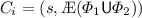
A single play from $(s,\varPhi )$ is a possibly infinite sequence of configurations $C_0 \rightarrow _{p_0} C_1 \rightarrow _{p_1} C_2 \rightarrow _{p_2} \ldots$, where $C_0=(s,\varPhi )$, $C_i \in S \times sub(\varPhi )$, and $p_i \in \{ \text {Player } \forall , \text {Player } \exists \}$. The subformula in $C_i$ determines which player $p_i$ makes the next move. The possible moves at each configuration are:

• (1) $C_i=(s,\textit{false})$, $C_i=(s,\textit{true})$, $C_i=(s,l)$: the play is finished. Such configurations are called terminal.

• (2) if $C_i=(s,A \bigcirc \varPhi )$, Player $\forall$ chooses a must-transition (for refutation) or a may-transition of $\mathcal {M}$ (to prevent satisfaction), and $C_{i+1}=(s',\varPhi )$.

• (3) if $C_i=(s,E \bigcirc \varPhi )$, Player $\exists$ chooses a must-transition (for satisfaction) or a may-transition of $\mathcal {M}$ (to prevent refutation), and $C_{i+1}=(s',\varPhi )$.

• (4) if $C_i=(s,\varPhi _1 \wedge \varPhi _2)$, then Player $\forall$ chooses $j \in \{1,2\}$ and $C_{i+1}=(s,\varPhi _j)$.

• (5) if $C_i=(s,\varPhi _1 \vee \varPhi _2)$, then Player $\exists$ chooses $j \in \{1,2\}$ and $C_{i+1}=(s,\varPhi _j)$.

• (6), (7) if , then .

• (8), (9) if , then .

The moves (6)–(9) are deterministic, thus any player can make them.

A play is a maximal play iff it is infinite or ends in a terminal configuration. A play is infinite [26] iff there is exactly one subformula of the form $A\textsf {U}$, $A\textsf {V}$, $E\textsf {U}$, or $E\textsf {V}$ that occurs infinitely often in the play. Such a subformula is called a witness. We have the following winning criteria:

• Player $\forall$ wins a (maximal) play iff in each configuration of the form $C_i=(s,A \bigcirc \varPhi )$, Player $\forall$ chooses a move based on must-transitions and one of the following holds: (1) the play is finite and ends in a terminal configuration of the form $C_i=(s,\textit{false})$ or $C_i=(s,a)$ where $a \not \in L(s)$ or $C_i=(s,\lnot a)$ where $a \in L(s)$; (2) the play is infinite and the witness is of the form $A\textsf {U}$ or $E\textsf {U}$.

• Player $\exists$ wins a (maximal) play iff in each configuration of the form $C_i=(s,E \bigcirc \varPhi )$, Player $\exists$ chooses a move based on must-transitions and one of the following holds: (1) the play is finite and ends in a terminal configuration of the form $C_i=(s,\textit{true})$ or $C_i=(s,a)$ where $a \in L(s)$ or $C_i=(s,\lnot a)$ where $a \not \in L(s)$; (2) the play is infinite and the witness is of the form $A\textsf {V}$ or $E\textsf {V}$.

• Otherwise, the play ends in a tie.

A strategy is a set of rules for a player, telling the player which move to choose in the current configuration. A winning strategy from $(s,\varPhi )$ is a set of rules allowing the player to win every play that starts at $(s,\varPhi )$ if he plays by the rules. It was shown in [24, 25] that the model checking problem of evaluating $[\mathcal {M}, s \models ^3 \varPhi ]$ can be reduced to the problem of finding which player has a winning strategy from $(s,\varPhi )$ (i.e. to solving the given 3-valued model checking game).

The algorithm proposed in [24, 25] for solving the given 3-valued model checking game consists of two parts. First, it constructs a game-graph, then it runs an algorithm for coloring the game-graph. The game-graph is $G_{\mathcal {M}\times \varPhi } = (N,E)$ where $N \subseteq S \times sub(\varPhi )$ is the set of nodes and $E \subseteq N \times N$ is the set of edges. N contains a node for each configuration that was reached during the construction of the game-graph that starts from initial configurations $I \times \{\varPhi \}$ in a BFS manner, and E contains an edge for each possible move that was applied. The nodes of the game-graph can be classified as: terminal nodes, $\wedge$-nodes, $\vee$-nodes, $A\bigcirc$-nodes, and $E\bigcirc$-nodes. Similarly, the edges can be classified as: progress edges, which originate in $A\bigcirc$ or $E\bigcirc$ nodes and reflect real transitions of the MTS $\mathcal {M}$, and auxiliary nodes, which are all other edges. We distinguish two types of progress edges, two types of children, and two types of SCCs (Strongly Connected Components). Must-edges (may-edges) are edges based on must-transitions (may-transitions) of MTSs. A node $n'$ is a must-child (may-child) of the node n if there exists a must-edge (may-edge) $(n,n')$. A must-SCC (may-SCC) is an SCC in which all progress edges are must-edges (may-edges).

The game-graph is partitioned into its may-Maximal SCCs (may-MSCCs), denoted $Q_i$’s. This partition induces a partial order $\le$ on the $Q_i$’s, such that edges go out of a set $Q_i$ only to itself or to a smaller set $Q_j$. The partial order is extended to a total order $\le$ arbitrarily. The coloring algorithm processes the $Q_i$’s according to $\le$, bottom-up. Let $Q_i$ be the smallest set that is not fully colored. The nodes of $Q_i$ are colored in two phases, as follows.

Phase 1. Apply these rules to all nodes in $Q_i$ until none of them is applicable.

• A terminal node C is colored: by T if Player $\exists$ wins in it (when $C=(s,\textit{true})$ or $C=(s,a)$ with $a \in L(s)$ or $C=(s,\lnot a)$ with $a \not \in L(s)$); and by F if Player $\forall$ wins in it (when $C=(s,\textit{false})$ or $C=(s,a)$ with $a \not \in L(s)$ or $C=(s,\lnot a)$ with $a \in L(s)$).

• An $A \bigcirc$ node is colored: by T if all its may-children are colored by T; by F if it has a must-child colored by F; by ? if all its must-children are colored by T or ?, and it has a may-child colored by F or ?.

• An $E \bigcirc$ node is colored: by T if it has a must-child colored by T; by F if all its may-children are colored by F; by ? if it has a may-child colored by T or ?, and all its must-children are colored by F or ?.

• An $\wedge$-node ($\vee$-node) is colored: by T (F) if both its children are colored by T (F); by F (T) if it has a child that is colored by F (T); by ? if it has a child colored by ? and the other child is colored by ? or T (F).

Phase 2. If after propagation of the rules of Phase 1, there are still nodes in $Q_i$ that remain uncolored, then $Q_i$ must be a non-trivial may-MSCC that has exactly one witness. We consider two cases.

• Case U. The witness is of the form $A(\varPhi _1 \textsf {U}\varPhi _2)$ or $E(\varPhi _1 \textsf {U}\varPhi _2)$.

  Phase 2a. Repeatedly color by ? each node in $Q_i$ that satisfies one of the following conditions, until there is no change:

  (1) An $A \bigcirc$ node that all its must-children are colored by T or ?; (2) An $E \bigcirc$ node that has a may-child colored by T or ?; (3) An $\wedge$ node that both its children are colored T or ?; (4) An $\vee$ node that has a child colored by T or ?.

  In fact, each node for which the F option is no longer possible according to the rules of Phase 1 is colored by ?.

  Phase 2b. Color the remaining nodes in $Q_i$ by F.

• Case V. The witness is of the form $A(\varPhi _1 \textsf {V}\varPhi _2)$ or $E(\varPhi _1 \textsf {V}\varPhi _2)$ (see [16, Appendix B]).

The result of the coloring is a 3-valued coloring function $\chi : N \rightarrow \{ T, F, ? \}$.

Theorem 2

([24]). For each $n = (s,\varPhi ') \in G_{\mathcal {M}\times \varPhi }$:

• (1) $[(\mathcal {M},s) \models ^3 \varPhi ']=\textit{tt}$ iff $\chi (n)=T$ iff Player $\exists$ has a winning strategy at n.

• (2) $[(\mathcal {M},s) \models ^3 \varPhi ']=\textit{ff}$ iff $\chi (n)=F$ iff Player $\forall$ has a winning strategy at n.

• (3) $[(\mathcal {M},s) \!\models ^3\! \varPhi ']\!=\!\!\bot$ iff $\chi (n)\!=?$ iff none of players has a winning strategy at n.

Using Theorems 1 and 2, given the colored game-graph of the MTS $\varvec{\alpha }^{ \text {join} }(\mathcal {F})$, if all its initial nodes are colored by T then $[\mathcal {F}\models \varPhi ] = \textit{tt}$, if at least one of them is colored by F then $[\mathcal {F}\models \varPhi ] = \textit{ff}$. Otherwise, we do not know.

Example 4

The colored game-graph for the MTS $\varvec{\alpha }^{ \text {join} }({\textsc {VendMach}})$ and $\varPhi _1=A (\lnot \textit{r} \textsf {U}\textit{r})$ is shown in Fig. 4. Green, red (with dashed borders), and white nodes denote nodes colored by T, F, and ?, respectively. The partitions from $Q_1$ to $Q_6$ consist of a single node shown in Fig. 4, while $Q_7$ contains all the other nodes. The initial node $(s_0,\varPhi _1)$ is colored by ?, so we obtain an indefinite answer.    $\square$

Fig. 4.

The colored game-graph for $\varvec{\alpha }^{ \text {join} }(\textsc {VendMach})$ and . (Color figure online)

5 Incremental Refinement Framework

Given an FTS $\pi _{\mathbb {K}'}(\mathcal {F})$ with a configuration set $\mathbb {K}' \subseteq \mathbb {K}$, we show how to exploit the game-graph of the abstract MTS $\mathcal {M}= \varvec{\alpha }^{ \text {join} }(\pi _{\mathbb {K}'}(\mathcal {F}))$ in order to do refinement in case that the model checking resulted in an indefinite answer. The refinement consists of two parts. First, we use the information gained by the coloring algorithm of $G_{\mathcal {M}\times \varPhi }$ in order to split the single abstract configuration $\textit{true}\in \varvec{\alpha }^{ \text {join} }(\mathbb {K}')$ that represents the whole concrete configuration set $\mathbb {K}'$. We then construct the refined abstract models, using the refined abstract configurations.

There are a failure node and a failure reason associated with an indefinite answer. The goal in the refinement is to find and eliminate at least one of the failure reasons.

Definition 5

A node n is a failure node if it is colored by ?, whereas none of its children was colored by ? at the time n got colored by the coloring algorithm.

Such failure node can be seen as the point where the loss of information occurred, so we can use it in the refinement step to change the final model checking result.

Fig. 5.

The refinement procedure that checks $[\mathcal {F}\models \varPhi ]$.

Lemma 1

([24]). A failure node is one of the following.

• An $A \bigcirc$-node ($E \bigcirc$-node) that has a may-child colored by F (T).

• An $A \bigcirc$-node ($E \bigcirc$-node) that was colored during Phase 2a based on an $A\textsf {U}$ ($A\textsf {V}$) witness, and has a may-child colored by ?.

Given a failure node $n=(s,\varPhi )$, suppose that its may-child is $n'=(s',\varPhi _1')$ as identified in Lemma 1. Then the may-edge from n to $n'$ is considered as the failure reason. Since the failure reason is a may-transition in the abstract MTS $\varvec{\alpha }^{ \text {join} }(\pi _{\mathbb {K}'}(\mathcal {F}))$, it needs to be refined in order to result either in a must transition or no transition at all. Let be the transition in the concrete model $\pi _{\mathbb {K}'}(\mathcal {F})$ corresponding to the above (failure) may-transition. We split the configuration space $\mathbb {K}'$ into $[\! [\psi ]\! ]$ and $[\! [\lnot \psi ]\! ]$ subsets, and we partition $\pi _{\mathbb {K}'}(\mathcal {F})$ in $\pi _{[\! [\psi ]\! ] \cap \mathbb {K}'}(\mathcal {F})$ and $\pi _{[\! [\lnot \psi ]\! ] \cap \mathbb {K}'}(\mathcal {F})$. Then, we repeat the verification process based on abstract models $\varvec{\alpha }^{ \text {join} }(\pi _{[\! [\psi ]\! ] \cap \mathbb {K}'}(\mathcal {F}))$ and $\varvec{\alpha }^{ \text {join} }(\pi _{[\! [\lnot \psi ]\! ] \cap \mathbb {K}'}(\mathcal {F}))$. Note that, in the former, $\varvec{\alpha }^{ \text {join} }(\pi _{[\! [\psi ]\! ] \cap \mathbb {K}'}(\mathcal {F}))$, becomes a must-transition, while in the latter, $\varvec{\alpha }^{ \text {join} }(\pi _{[\! [\lnot \psi ]\! ] \cap \mathbb {K}'}(\mathcal {F}))$, is removed. The complete refinement procedure is shown in Fig. 5. We prove that (see [16, Appendix A]):

Theorem 3

The procedure terminates and is correct.

Example 5

We can do a failure analysis on the game-graph of $\varvec{\alpha }^{ \text {join} }(\textsc {VendMach})$ in Fig. 4. The failure node is $(s_1,A \bigcirc A (\lnot \textit{r} \textsf {U}\textit{r}))$ and the reason is the may-edge . The corresponding concrete transition in VendMach is . So, we partition the configuration space $\displaystyle \mathbb {K}^{\textsc {VM}}$ into subsets and , and in the next second iteration we consider FTSs and .    $\square$

Fig. 6.

.

Fig. 7.

The game-based model checking algorithm provides us with a convenient framework to use results from previous iterations and avoid unnecessary calculations. At the end of the i-th iteration of abstraction-refinement, we remember those nodes that were colored by definite colors. Let D denote the set of such nodes. Let $\chi _D: D \rightarrow \{ T, F \}$ be the coloring function that maps each node in D to its definite color. The incremental approach uses this information both in the construction of the game-graph and its coloring. During the construction of a new refined game-graph performed in a BFS manner in the next $i+1$-th iteration, we prune the game-graph in nodes that are from D. When a node $n \in D$ is encountered, we add n to the game-graph and do not continue to construct the game-graph from n onwards. That is, $n \in D$ is considered as terminal node and colored by its previous color. As a result of this pruning, only the reachable sub-graph that was previously colored by ? is refined.

Example 6

The property $\varPhi _1$ holds for . The initial node of the game-graph (see [16, Fig. 13, Appendix C]), is colored by T. On the other hand, we obtain an indefinite answer for . The model is shown in Fig. 7, whereas the final colored game-graph is given in Fig. 6. The failure node is $(s_0,A \bigcirc A (\lnot \textit{r} \textsf {U}\textit{r}))$, and the reason is the may-edge . The corresponding concrete transition in is . So, in the next third iteration we consider FTSs and .

The initial node of the graph (see [16, Fig. 16, Appendix C]) is colored by F in Phase 2b. The initial node of (see [16, Fig. 17, Appendix C]) is colored by T.

In the end, we conclude that $\varPhi _1$ is satisfied by the variants , and $\varPhi$ is violated by the variant .

On the other hand, we need two iterations to conclude that $\varPhi _2=E (\lnot \textit{r} \textsf {U}\textit{r})$ is satisfied by all variants in $\displaystyle \mathbb {K}^{\textsc {VM}}$ (see [16, Appendix D] for details).    $\square$

Fig. 8.

The model $M_2$.

Fig. 9.

Verification of $M_n$ (T in seconds).

6 Evaluation

To evaluate our approach, we use a synthetic example to demonstrate specific characteristics of our approach, and the Elevator  model which is often used as benchmark in SPL community [4, 12, 15, 20, 23]. We compare (1) our abstraction-refinement procedure Verify with the game-based model checking algorithm implemented in Java from scratch vs. (2) family-based version of the NuSMVmodel checker, denoted fNuSMV, which implements the standard lifted model checking algorithm [5]. For each experiment, we measure T(ime) to perform an analysis task, and Call which is the number of times an approach calls the model checking engine. All experiments were executed on a 64-bit Intel$^\circledR$Core$^{TM}$ i5-3337U CPU running at 1.80 GHz with 8 GB memory. All experimental data is available from: https://aleksdimovski.github.io/automatic-ctl.html.

Synthetic example. The FTS $M_n$ (where $n>0$) consists of n features $A_1, \ldots , A_n$ and an integer data variable x, such that the set AP consists of all evaluations of x which assign nonnegative integer values to x. The set of valid configurations is $\mathbb {K}_{n} = 2^{\{A_1, \ldots , A_n\}}$. $M_n$ has a tree-like structure, where in the root is the initial state with $x=0$. In each level k ($k \ge 1$), there are two states that can be reached with two transitions leading from a state from a previous level. One transition is allowable for variants with the feature $A_k$ enabled, so that in the target state the variable’s value is $x+2^{k-1}$ where x is its value in the source state, whereas the other transition is allowable for variants with $A_k$ disabled, so that the value of x does not change. For example, $M_2$ is shown in Fig. 8, where in each state we show the current value of x and all transitions have the silent action $\tau$.

We consider two properties: $\varPhi = A (\textit{true}\,\textsf {U}(x \!\ge \! 0))$ and $\varPhi ' = A (\textit{true}\,\textsf {U}(x \!\ge \! 1))$. The property $\varPhi$ is satisfied by all variants in $\mathbb {K}$, whereas $\varPhi '$ is violated only by one configuration $\lnot A_1 \!\wedge \! \ldots \!\wedge \! \lnot A_n$ (where all features are disabled). We have verified $M_n$ against $\varPhi$ and $\varPhi '$ using fNuSMV (e.g. see fNuSMVmodels for $M_1$ and $M_2$ in [16, Fig. 23, Appendix E]). We have also checked $M_n$ using our Verify procedure. For $\varPhi$, Verify terminates in one iteration since $\varvec{\alpha }^{ \text {join} }(M_n)$ satisfies $\varPhi$ (see $G_{\varvec{\alpha }^{ \text {join} }(M_1) \times \varPhi }$ in [16, Fig. 24, Appendix E]). For $\varPhi '$, Verify needs $n+1$ iterations. First, an indefinite result is reported for $\varvec{\alpha }^{ \text {join} }(M_n)$ (e.g. see $G_{\varvec{\alpha }^{ \text {join} }(M_1) \times \varPhi '}$ in [16, Fig. 27, Appendix E]), and the configuration space is split into $[\! [\lnot A_1 ]\! ]$ and $[\! [A_1 ]\! ]$ subsets. The refinement procedure proceeds in this way until we obtain definite results for all variants. The performance results are shown in Fig. 9. Notice that, fNuSMV reports all results in only one iteration. As n grows, Verify becomes faster than fNuSMV. For $n=11$ ($|\mathbb {K}|=2^{11}$), fNuSMV  timeouts after 2 h. In contrast, Verify is feasible even for large values of n.

Elevator. We have experimented with the Elevator model with four floors, designed by Plath and Ryan [23]. It contains about 300 LOC of fNuSMV code and 9 independent optional features that modify the basic behaviour of the elevator, thus yielding $2^9$ = 512 variants. To use our Verify procedure, we have manually translated the fNuSMV model into an FTS and then we have called Verify on it. The basic Elevator system consists of a single lift that travels between four floors. There are four platform buttons and a single lift, which declares variables floor, door, direction, and a further four cabin buttons. When serving a floor, the lift door opens and closes again. We consider three properties “$\varPhi _1=E (\textit{tt}\, \textsf {U}(floor\!=\!1 \wedge idle \wedge door\!=\!closed))$”, “$\varPhi _2=A (\textit{tt}\, \textsf {U}(floor\!=\!1 \wedge idle \wedge door\!=\!closed))$”, and “$\varPhi _3=E (\textit{tt}\, \textsf {U}((floor\!=\!3 \wedge \lnot liftBut3.pressed \wedge direction\!=\!up) \implies door\!=\!closed))$”. The performance results are shown in Fig. 10. The properties $\varPhi _1$ and $\varPhi _2$ are satisfied by all variants, so Verify achieves speed-ups of 28 times for $\varPhi _1$ and 2.7 times for $\varPhi _2$ compared to the fNuSMV approach. fNuSMV takes 1.76 sec to check $\varPhi _3$, whereas Verify ends in 0.67 sec thus giving 2.6 times performance speed-up.

Fig. 10.

Verification of Elevator  properties (T in seconds).

7 Related Work and Conclusion

There are different formalisms for representing variability models [2, 21]. Classen et al. [4] present Featured Transition Systems (FTSs). They show how specifically designed lifted model checking algorithms [5, 7] can be used for verifying FTSs against LTL and CTL properties. The variability abstractions that preserve LTL are introduced in [14, 15, 17], and subsequently automatic abstraction refinement procedures [8, 18] for lifted model checking of LTL are proposed, by using Craig interpolation to define the refinement. The variability abstractions that preserve the full CTL are introduced in [12], but they are constructed manually and no notion of refinement is defined there. In this paper, we define an automatic abstraction refinement procedure for lifted model checking of full CTL by using games to define the refinement. To the best of our knowledge, this is the first such procedure in lifted model checking.

One of the earliest attempts for using games for CTL model checking has been proposed by Stirling [26]. Shoham and Grumberg [3, 19, 24, 25] have extended this game-based approach for CTL over 3-valued semantics. In this work, we exploit and apply the game-based approach in a completely new direction, for automatic CTL verification of variability models.

The works [11, 13] present an approach for software lifted model checking of #ifdef-based program families using symbolic game semantics models [10].

To conclude, in this work we present a game-based lifted model checking for abstract variability models with respect to the full CTL. We also suggest an automatic refinement procedure, in case the model checking result is indefinite.

References

Baier, C., Katoen, J.: Principles of Model Checking. MIT Press, Cambridge (2008)
ter Beek, M.H., Fantechi, A., Gnesi, S., Mazzanti, F.: Modelling and analysing variability in product families: model checking of modal transition systems with variability constraints. J. Log. Algebr. Methods Program. 85(2), 287–315 (2016). https://doi.org/10.1016/j.jlamp.2015.09.004
Campetelli, A., Gruler, A., Leucker, M., Thoma, D.: Don’t Know for multi-valued systems. In: Liu, Z., Ravn, A.P. (eds.) ATVA 2009. LNCS, vol. 5799, pp. 289–305. Springer, Heidelberg (2009). https://doi.org/10.1007/978-3-642-04761-9_22
Classen, A., Cordy, M., Schobbens, P., Heymans, P., Legay, A., Raskin, J.: Featured transition systems: foundations for verifying variability-intensive systems and their application to LTL model checking. IEEE Trans. Softw. Eng. 39(8), 1069–1089 (2013). http://doi.ieeecomputersociety.org/10.1109/TSE.2012.86
Classen, A., Heymans, P., Schobbens, P.Y., Legay, A.: Symbolic model checking of software product lines. In: Proceedings of the 33rd International Conference on Software Engineering, ICSE 2011, pp. 321–330. ACM (2011). http://doi.acm.org/10.1145/1985793.1985838
Clements, P., Northrop, L.: Software Product Lines: Practices and Patterns. Addison-Wesley, Boston (2001)
Cordy, M., Classen, A., Heymans, P., Schobbens, P., Legay, A.: Provelines: a product line of verifiers for software product lines. In: 17th International SPLC 2013 Workshops, pp. 141–146. ACM (2013). http://doi.acm.org/10.1145/2499777.2499781
Cordy, M., Heymans, P., Legay, A., Schobbens, P., Dawagne, B., Leucker, M.: Counterexample guided abstraction refinement of product-line behavioural models. In: Proceedings of the 22nd ACM SIGSOFT International Symposium on Foundations of Software Engineering, (FSE-22), pp. 190–201. ACM (2014). http://doi.acm.org/10.1145/2635868.2635919
Cousot, P.: Partial completeness of abstract fixpoint checking. In: Choueiry, B.Y., Walsh, T. (eds.) SARA 2000. LNCS (LNAI), vol. 1864, pp. 1–25. Springer, Heidelberg (2000). https://doi.org/10.1007/3-540-44914-0_1
Dimovski, A.S.: Program verification using symbolic game semantics. Theor. Comput. Sci. 560, 364–379 (2014). https://doi.org/10.1016/j.tcs.2014.01.016
Dimovski, A.S.: Symbolic game semantics for model checking program families. In: Bošnački, D., Wijs, A. (eds.) SPIN 2016. LNCS, vol. 9641, pp. 19–37. Springer, Cham (2016). https://doi.org/10.1007/978-3-319-32582-8_2
Dimovski, A.S.: Abstract family-based model checking using modal featured transition systems: preservation of CTL\(^{\star }\). In: Russo, A., Schürr, A. (eds.) FASE 2018. LNCS, vol. 10802, pp. 301–318. Springer, Cham (2018). https://doi.org/10.1007/978-3-319-89363-1_17
Dimovski, A.S.: Verifying annotated program families using symbolic game semantics. Theor. Comput. Sci. 706, 35–53 (2018). https://doi.org/10.1016/j.tcs.2017.09.029
Dimovski, A.S., Al-Sibahi, A.S., Brabrand, C., Wąsowski, A.: Family-based model checking without a family-based model checker. In: Fischer, B., Geldenhuys, J. (eds.) SPIN 2015. LNCS, vol. 9232, pp. 282–299. Springer, Cham (2015). https://doi.org/10.1007/978-3-319-23404-5_18
Dimovski, A.S., Al-Sibahi, A.S., Brabrand, C., Wasowski, A.: Efficient family-based model checking via variability abstractions. STTT 19(5), 585–603 (2017). https://doi.org/10.1007/s10009-016-0425-2
Dimovski, A.S., Legay, A., Wasowski, A.: Variability abstraction and refinement for game-based lifted model checking of full CTL (extended version). CoRR (2019). http://arxiv.org/
Dimovski, A.S., Wąsowski, A.: From transition systems to variability models and from lifted model checking back to UPPAAL. In: Aceto, L., Bacci, G., Bacci, G., Ingólfsdóttir, A., Legay, A., Mardare, R. (eds.) Models, Algorithms, Logics and Tools. LNCS, vol. 10460, pp. 249–268. Springer, Cham (2017). https://doi.org/10.1007/978-3-319-63121-9_13
Dimovski, A.S., Wąsowski, A.: Variability-specific abstraction refinement for family-based model checking. In: Huisman, M., Rubin, J. (eds.) FASE 2017. LNCS, vol. 10202, pp. 406–423. Springer, Heidelberg (2017). https://doi.org/10.1007/978-3-662-54494-5_24
Grumberg, O., Lange, M., Leucker, M., Shoham, S.: When not losing is better than winning: abstraction and refinement for the full mu-calculus. Inf. Comput. 205(8), 1130–1148 (2007). https://doi.org/10.1016/j.ic.2006.10.009
Iosif-Lazar, A.F., Melo, J., Dimovski, A.S., Brabrand, C., Wasowski, A.: Effective analysis of c programs by rewriting variability. Program. J. 1(1), 1 (2017). https://doi.org/10.22152/programming-journal.org/2017/1/1
Larsen, K.G., Nyman, U., Wąsowski, A.: Modal I/O automata for interface and product line theories. In: De Nicola, R. (ed.) ESOP 2007. LNCS, vol. 4421, pp. 64–79. Springer, Heidelberg (2007). https://doi.org/10.1007/978-3-540-71316-6_6
Larsen, K.G., Thomsen, B.: A modal process logic. In: Proceedings of the Third Annual Symposium on Logic in Computer Science (LICS 1988), pp. 203–210. IEEE Computer Society (1988). http://dx.doi.org/10.1109/LICS.1988.5119
Plath, M., Ryan, M.: Feature integration using a feature construct. Sci. Comput. Program. 41(1), 53–84 (2001). https://doi.org/10.1016/S0167-6423(00)00018-6
Shoham, S., Grumberg, O.: A game-based framework for CTL counterexamples and 3-valued abstraction-refinement. ACM Trans. Comput. Log. 9(1), 1 (2007). https://doi.org/10.1145/1297658.1297659
Shoham, S., Grumberg, O.: Compositional verification and 3-valued abstractions join forces. Inf. Comput. 208(2), 178–202 (2010). https://doi.org/10.1016/j.ic.2009.10.002
Stirling, C.: Modal and Temporal Properties of Processes. Texts in Computer Science. Springer, New York (2001). https://doi.org/10.1007/978-1-4757-3550-5
Author information
Authors and Affiliations
Corresponding author
Editor information
Editors and Affiliations
Rights and permissions
Open Access This chapter is licensed under the terms of the Creative Commons Attribution 4.0 International License (http://creativecommons.org/licenses/by/4.0/), which permits use, sharing, adaptation, distribution and reproduction in any medium or format, as long as you give appropriate credit to the original author(s) and the source, provide a link to the Creative Commons license and indicate if changes were made.
The images or other third party material in this chapter are included in the chapter's Creative Commons license, unless indicated otherwise in a credit line to the material. If material is not included in the chapter's Creative Commons license and your intended use is not permitted by statutory regulation or exceeds the permitted use, you will need to obtain permission directly from the copyright holder.
Copyright information
© 2019 The Author(s)
About this paper
Cite this paper
Dimovski, A.S., Legay, A., Wasowski, A. (2019). Variability Abstraction and Refinement for Game-Based Lifted Model Checking of Full CTL. In: Hähnle, R., van der Aalst, W. (eds) Fundamental Approaches to Software Engineering. FASE 2019. Lecture Notes in Computer Science(), vol 11424. Springer, Cham. https://doi.org/10.1007/978-3-030-16722-6_11
Download citation
DOI: https://doi.org/10.1007/978-3-030-16722-6_11
Published:
Publisher Name: Springer, Cham
Print ISBN: 978-3-030-16721-9
Online ISBN: 978-3-030-16722-6
eBook Packages: Computer ScienceComputer Science (R0)