
Abstract
In recent years, asymptotic approximation schemes have been developed to describe the motion of a small compact object through a vacuum background to any order in perturbation theory. The schemes are based on rigorous methods of matched asymptotic expansions, which account for the object’s finite size, require no “regularization” of divergent quantities, and are valid for strong fields and relativistic speeds. Up to couplings of the object’s multipole moments to the external background curvature, these schemes have established that at least through second order in perturbation theory, the object’s motion satisfies a generalized equivalence principle: it moves on a geodesic of a certain smooth metric satisfying the vacuum Einstein equation. I describe the foundations of this result, particularly focusing on the fundamental notion of how a small object’s motion is represented in perturbation theory. The three common representations of perturbed motion are (i) the “Gralla-Wald” description in terms of small deviations from a reference geodesic, (ii) the “self-consistent” description in terms of a worldline that obeys a self-accelerated equation of motion, and (iii) the “osculating geodesics” description, which utilizes both (i) and (ii). Because of the coordinate freedom in general relativity, any coordinate desscription of motion in perturbation theory is intimately related to the theory’s gauge freedom. I describe asymptotic solutions of the Einstein equations adapted to each of the three representations of motion, and I discuss the gauge freedom associated with each. I conclude with a discussion of how gauge freedom must be refined in the context of long-term dynamics.
Access this chapter
Tax calculation will be finalised at checkout
Purchases are for personal use only
Notes
- 1.
In a certain sense, an object’s mass affects its own motion even in a Newtonian binary. Each object follows a Keplerian orbit about the system’s center of mass, not about the center of the other object. Since the center of mass is shifted by the object’s own mass, the object affects its own motion; more plainly, \(m_1\) influences its own motion by influencing that of \(m_2\). This is a more indirect effect than the type described above, but in practice, distinguishing it from any other post-test-body effect is nontrivial. See Ref. [4] for a discussion.
- 2.
Of course, once the two bodies are sufficiently close to each other, they interact in a highly nonlinear, highly relativistic way. In that regime, one must use numerical relativity to solve the fully nonlinear Einstein equations for the system.
- 3.
- 4.
I refer the reader to Appendix 1 for the expansion of the geodesic equation in powers of a metric perturbation.
- 5.
Another compelling physical interpretation is provided by Quinn and Wald [24]. They showed that the MiSaTaQuWa equation follows from the assumption that the net force is equal to an average over a certain “bare” force over a sphere around the particle. (This assumption was later proved to be true in a large class of gauges [18, 19, 31].) In the language of Detweiler and Whiting fields, the force lines of the singular field are symmetric around the particle and vanish upon averaging, while the force lines of the regular field are asymmetric and add up to a net force on the particle.
- 6.
More precisely, it is governed by Eq. (35).
- 7.
- 8.
In the Lorenz gauge in a vacuum background, the linearized curvature tensors are related by \(E_{\mu \nu }[h]=-2\delta R_{\mu \nu }[h]=-2\overline{\delta G_{\mu \nu }[h]}=\overline{E_{\mu \nu }[\bar{h}]}\).
- 9.
Cross terms like \(\delta ^2R_{\mu \nu }[h^1,h^2]\) are as defined in Eq. (227).
- 10.
Equation (222) illustrates more explicitly, using a point-particle field, how the gauge condition implies an equation of motion.
- 11.
It also constrains other quantities in \(h_{\mu \nu }\), particularly determining the evolution of the object’s mass and spin.
- 12.
Note that although a puncture scheme utilizes approximations to \(h^\mathrm{S}_{\mu \nu }\) and \(h^\mathrm{R}_{\mu \nu }\), it is designed to exactly obtain \(h^\mathrm{R}_{\mu \nu }\) (and any finite number of its derivatives) on the worldline, meaning it does not introduce any approximation into the motion of \(\gamma _\epsilon \). Nor does it introduce approximations into the physical field \(h_{\mu \nu }=h^\mathrm{R}_{\mu \nu }+h^\mathrm{S}_{\mu \nu }=h^\mathcal {R}_{\mu \nu }+h^\mathcal {P}_{\mu \nu }\).
- 13.
Here I return to what will become my common practice of dropping the subscript \(\epsilon \) on \(z^\mu \) for simplicity, though I refer to the self-consistently determined center-of-mass worldline, not the freely specifiable worldline for which the relaxed Einstein equation can be solved.
- 14.
- 15.
The scheme I describe here should not be confused with the general method of osculating geodesics, which is simply a way of using instantaneously tangential geodesics to rewrite an equation of motion \(\frac{D^2z^\mu }{d\tau ^2}=F^\mu \) in terms of more convenient variables; that general method, inherited from celestial mechanics, is exact and does not inherently involve an expansion of \(z^\mu \), although it is particularly well suited to the osculating-geodesic approximation discussed here [59].
- 16.
In truth, it is unlikely that any of the expansions I consider, whether self-consistent, Gralla-Wald, or osculating-geodesics, is convergent. More likely, they are asymptotic approximations only. So when performing the self-consistent expansion, I actually assume that \(|{\text{ g }}_{\mu \nu }(x,\epsilon )-{\text{ g }}^N_{\mu \nu }(x,\epsilon ;z)|=o(\epsilon ^N)\), where \({\text{ g }}^N_{\mu \nu }(x,\epsilon ;z)=g_{\mu \nu }(x)+\sum _{n=1}^N\epsilon ^n h^n_{\mu \nu }(x;z)\). The notation \(o(k(\epsilon ))\) means “goes to zero faster than \(k(\epsilon )\)”.
- 17.
Here indices refer to the unscaled coordinates \((t,x^i)\). If components are written in the scaled coordinates, overall factors \(\epsilon \) and \(\epsilon ^2\) appear in front of \(ta\) and \(ab\) components, respectively. These overall factors have no practical impact.
- 18.
This matching condition amounts to the assumption that nothing too “funny” happens in the buffer region. It can instead be replaced by more explicit assumptions on the behavior of the full metric \({\text{ g }}_{\mu \nu }\), such as the conditions assumed in Ref. [18] or various others discussed in Ref. [41].
- 19.
\(\ln r\) terms also generically arise. For simplicity, I incorporate those terms into \(h^{np}_{\mu \nu }\) for the moment. Their presence does not spoil the well-orderedness of the expansion, since \(r^p(\ln r)^q\ll r^{p'}(\ln r)^{q'}\) for \(p>p'\). Similarly, \(\ln \epsilon \) terms can occur in solving the relaxed Einstein equation [15], and I absorb them into the coefficients \(h^n_{\mu \nu }(x;z)\).
- 20.
The fact that the inner background must be asymptotically flat, containing no positive powers of \(r\), follows from the assumption that the outer expansion contains no negative powers of \(\epsilon \), in the same manner as the cutoff on powers of \(1/r\) in Eq. (41).
- 21.
This notion of mass-centeredness based on the mass dipole moment of \(g^\mathrm{obj}_{\mu \nu }\) applies only to order-\(\epsilon \) deviations from \(z^\mu \). For higher-order deviations, mass-dipole-moment terms in the perturbations \(H^n_{\mu \nu }\) must also be considered, or some other copacetic centeredness condition must be imposed, as discussed in Sects. 3 and 7.
- 22.
Intuitively, the logarithms are caused by the object perturbing the spacetime’s light cones. One can expect the solution to the exact Einstein equation to propagate on (and within) null cones of the exact spacetime, and given that the mass of the body induces a logarithmic correction to the retarded time, logarithmic corrections then naturally appear in \(h_{\mu \nu }^n\). This effect is well known from solutions to the Einstein equation in harmonic coordinates (see, e.g., Refs. [66, 67]). For generality, I allow logarithms at any value of \(n\), but I assume that for each finite \(n\), \(p\), and \(\ell \), the highest power of \(\ln r\) is a finite number \({q_\mathrm{max}}(n,p,\ell )\). For simplicity, to make sure that term-by-term differentiation is valid without worrying about issues of convergence, I also assume for a given, finite \(n\) and \(p\), \(\ell \) has a maximum \({\ell _\mathrm{max}}(n,p)\).
- 23.
To relate back to the Thorne and Hartle results (13) and (14), canonical mass and current quadrupole moments \(Q_{ij}\) and \(\mathcal {Q}_{ij}\) can be defined from \(M^3_{\mu \nu ij}\) and \(S^3_{\mu \nu ij}\) according to

similarly to Eq. (63). In choosing the normalization factors of these moments, I follow Ref. [68].
- 24.
A proof of statement (iii) will be presented elsewhere. Here it can be taken as a conjecture, although it is known to be true at all orders in \(\epsilon \) and \(r\) that have been explicitly considered. Intuitively, it can be inferred from the fact that we can choose boundary conditions for which all \(k^n_{\mu \nu L}\) vanish at a given \(n\), and with that choice we must still be able to satisfy the gauge condition; hence, the constraints on the \(I^n_{\mu \nu L}\)’s cannot involve the \(k^n_{\mu \nu L}\)’s of the same \(n\).
- 25.
If the statements were not true, one could always slightly alter the singular-regular split to make the two fields independently satisfy the gauge condition. Doing so would involve appropriately moving part of the free fields into \(h^\mathrm{S}_{\mu \nu }\) [15].
- 26.
The monopole correction (64) can also be trivially rewritten in terms of \(h^{\mathrm{R}1}_{\mu \nu }\) as

where I have set \(M^i=0\), and all fields are evaluated on \(\gamma .\)
- 27.
That it must be well defined as a distribution follows from it being the result of linear operations on \(h_{\mu \nu }^\mathrm{seed}[I^n_\ell ]\), and \(h_{\mu \nu }^\mathrm{seed}[I^n_\ell ]\) itself being a sum of terms constructed from linear operations on an integrable function. The latter fact follows from the first term in the sum being expressible as the linear operation \(\partial _L\) on an integrable function proportional to \(r^{-1}\) [as in the text above Eq. (86)], and all higher-order terms in the sum being constructed from linear operations on lower order terms in the sum (as described in Sect. 3.2).
- 28.
One does not solve the problem in each domain separately, since the separate problems would be ill-posed. Instead, when calculating \(h^n_{\mu \nu }\) at a point just outside \(\Gamma \) that depends on points on past time slices inside \(\Gamma \), one makes use of the values of \(h^{\mathcal {R}n}_{\mu \nu }\) already calculated at those earlier points, and vice versa; see Sect. VB of Ref. [54].
- 29.
The effective sources \(S^{\mathrm{eff}n}_{\mu \nu }\) are usually written to include the skeletal stress-energy terms, which are canceled by distributional content in \(E_{\mu \nu }[h^{\mathcal {P}n}]\). Here I have instead followed Ref. [20] by writing the source pointwise, off \(\gamma \); if the puncture agrees with the singular field sufficiently well, the source at points on \(\gamma \) can be defined as the limit from off \(\gamma \).
- 30.
Because the approximation is accurate only within a finite region of size \(1/\epsilon \), one might better solve the equations in the future domain of dependence of a partial Cauchy surface.
- 31.
Since the approximation is held to be valid in a region of size \(\varsigma (\epsilon )\ll 1/\sqrt{\epsilon }\), a reasonable approach would be to solve the equations in the causal future of a partial Cauchy surface of that size.
- 32.
The extension of Gralla and Wald’s result to the self-consistent case [12] unfortunately contained a significant error, leading to a result that held only in gauges continuously related to Lorenz, as in the Barack-Ori analysis.
- 33.
At this stage the transformation is applied only to the sums \(\check{h}^n_{\mu \nu }=\check{h}^{\mathrm{R}n}_{\mu \nu }+\check{h}^{\mathrm{S}n}_{\mu \nu }\); one does not yet need transformation laws for the individual pieces \(\check{h}^{\mathrm{R}n}_{\mu \nu }\) and \(\check{h}^{\mathrm{S}n}_{\mu \nu }\).
- 34.
Rather than saying the equation of motion (35) is invariant, self-force literature usually talks about a transformation of the self-force. At first order, the equation in the new gauge is \(\frac{D^2z'^\mu _{1\perp }}{d\tau _0^2}+R^\mu _{\alpha \nu \beta }u_0^\alpha z'^\nu _{1\perp }u_0^\beta =\check{F}'^\mu _1\). The force is given by
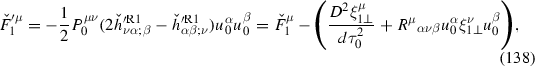
where the second equality follows from \(\check{h}'^{\mathrm{R}1}_{\mu \nu }=\check{h}^{\mathrm{R}1}_{\mu \nu }+\mathcal {L}_{\xi _1}g_{\mu \nu }\). With \(z'^\mu _{1\perp }=z_{1\perp }^\mu -\epsilon \xi _{1\perp }^\mu \) in the left-hand side of the equation of motion, the equation’s invariance is transparent.
- 35.
Note that without some additional input beyond that definition, the split of \({\text{ g }}_{\mu \nu }\) into \(g_{\mu \nu }\), \(\mathfrak {h}^\mathrm{R}_{\mu \nu }\), and \(\mathfrak {h}^\mathrm{S}_{\mu \nu }\) is quite ambiguous. Suppose there were a zeroth-order force acting on the object. One could still write the equation of motion as a geodesic in some smooth piece of the metric, but to do so, one would have to shift part of \(g_{\mu \nu }\) into \(\mathfrak {h}^\mathrm{S}_{\mu \nu }\); one would not simply be splitting the perturbations \(h'^n_{\mu \nu }\). With the present setup, the ambiguity is lifted by assuming the expansion (25) and utilizing the independently determined fact that \(F_0^\mu =0\).


References
R. Geroch, J. Traschen, Strings and other distributional sources in general relativity. Phys. Rev. D 36, 1017–1031 (1987)
R. Steinbauer, J.A. Vickers, On the Geroch-Traschen class of metrics. Class. Quantum Gravity 26, 065001 (2009)
A. Einstein, L. Infeld, B. Hoffmann, The gravitational equations and the problem of motion. Ann. Math. 39, 65–100 (1938)
S. Detweiler, Perspective on gravitational self-force analyses. Class. Quantum Gravity 22, S681–S716 (2005)
L. Blanchet, Gravitational radiation from post-Newtonian sources and inspiralling compact binaries. Living Rev. Relativ. 17, 2 (2014)
T. Futamase, Y. Itoh, The post-Newtonian approximation for relativistic compact binaries. Living Rev. Relativ. 10, 2 (2007)
E. Poisson, C.M. Will, Gravity: Newtonian, Post-Newtonian, and Relativistic (Cambridge University Press, Cambridge, 2014)
L. Barack, Gravitational self force in extreme mass-ratio inspirals. Class. Quantum Gravity 26, 213001 (2009)
E. Poisson, A. Pound, I. Vega, The motion of point particles in curved spacetime. Living Rev. Relativ. 14, 7 (2011)
P. Amaro-Seoane, J.R. Gair, A. Pound, S.A. Hughes, C.F. Sopuerta, Research Update on Extreme-Mass-Ratio Inspirals (2014)
A. Pound, Self-consistent gravitational self-force. Phys. Rev. D 81(2), 024023 (2010)
A. Pound, Singular perturbation techniques in the gravitational self-force problem. Phys. Rev. D 81, 124009 (2010)
A. Pound, Motion of small bodies in general relativity: foundations and implementations of the self-force. Ph.D. thesis, University of Guelph (2010)
A. Pound, Second-order gravitational self-force. Phys. Rev. Lett. 109, 051101 (2012)
A. Pound, Nonlinear gravitational self-force: field outside a small body. Phys. Rev. D 86, 084019 (2012)
A. Pound, Nonlinear gravitational self-force: second-order equation of motion. In preparation
A. Pound, Gauge and motion in perturbation theory. In preparation
S.E. Gralla, R.M. Wald, A rigorous derivation of gravitational self-force. Class. Quantum Gravity 25, 205009 (2008)
S.E. Gralla, Gauge and averaging in gravitational self-force. Phys. Rev. D 84, 084050 (2011)
S.E. Gralla, Second order gravitational self force. Phys. Rev. D 85, 124011 (2012)
Y. Mino, M. Sasaki, T. Tanaka, Gravitational radiation reaction to a particle motion. Phys. Rev. D 55, 3457–3476 (1997)
S.L. Detweiler, Radiation reaction and the self-force for a point mass in general relativity. Phys. Rev. Lett. 86, 1931–1934 (2001)
S.L. Detweiler, B.F. Whiting, Self-force via a Green’s function decomposition. Phys. Rev. D 67, 024025 (2003)
T.C. Quinn, R.M. Wald, An axiomatic approach to electromagnetic and gravitational radiation reaction of particles in curved space-time. Phys. Rev. D 56, 3381–3394 (1997)
S.E. Gralla, A.I. Harte, R.M. Wald, A rigorous derivation of electromagnetic self-force. Phys. Rev. D 80, 024031 (2009)
A.I. Harte, Self-forces from generalized killing fields. Class. Quantum Gravity 25, 235020 (2008)
A.I. Harte, Electromagnetic self-forces and generalized killing fields. Class. Quantum Gravity 26, 155015 (2009)
A.I. Harte, Motion in classical field theories and the foundations of the self-force problem (2014)
T.M. Linz, J.L. Friedman, A.G. Wiseman, Combined gravitational and electromagnetic self-force on charged particles in electrovac spacetimes (2014)
P. Zimmerman, E. Poisson, Gravitational self-force in nonvacuum spacetimes (2014)
A. Pound, C. Merlin, L. Barack, Gravitational self-force from radiation-gauge metric perturbations. Phys. Rev. D 89, 024009 (2014)
C.R. Galley, B.L. Hu, Self-force on extreme mass ratio inspirals via curved spacetime effective field theory. Phys. Rev. D 79, 064002 (2009)
C.R. Galley, A Nonlinear scalar model of extreme mass ratio inspirals in effective field theory II. Scalar perturbations and a master source. Class. Quantum Gravity 29, 015011 (2012)
W.G. Dixon, Dynamics of extended bodies in general relativity. iii. equations of motion. Phil. Trans. R. Soc. Lond. A 277, 59 (1974)
M. Mathisson, Neue mechanik materieller systeme. Acta Phys. Pol. 6, 163 (1937)
A.I. Harte, Mechanics of extended masses in general relativity. Class. Quantum Gravity 29, 055012 (2012)
J. Ehlers, E. Rudolph, Dynamics of extended bodies in general relativity: center-of-mass description and quasirigidity. Gen. Relativ. Gravit. 8, 197–217 (1977)
A.I. Harte, Effective stress-energy tensors, self-force, and broken symmetry. Class. Quantum Gravity 27, 135002 (2010)
J. Kevorkian, J.D. Cole, Multiple Scale and Singular Perturbation Methods (Springer, New York, 1996)
N. Fenichel, Geometric singular perturbation theory for ordinary differential equations. J. Differ. Equ. 31(1), 53–98 (1979)
W. Eckhaus, Asymptotic Analysis of Singular Perturbations (Elsevier North-Holland, New York, 1979)
R.E. Kates, Underlying structure of singular perturbations on manifolds. Ann. Phys. (N.Y.) 132, 1–17 (1981)
P. D’Eath, Dynamics of a small black hole in a background universe. Phys. Rev. D 11, 1387 (1975)
P.D. D’Eath, Black Holes: Gravitational Interactions (Oxford University Press, New York, 1996)
R.E. Kates, Motion of a small body through an external field in general relativity calculated by matched asymptotic expansions. Phys. Rev. D 22, 1853 (1980)
K.S. Thorne, J.B. Hartle, Laws of motion and precession for black holes and other bodies. Phys. Rev. D 31, 1815 (1985)
H. Weyl, Raum, Zeit, Materie, 4th edn., Chapter 36 (Springer, Berlin, 1921)
A. Einstein, J. Grommer, Allgemeine relativitätstheorie und bewegungsgesetz. Sitzungsber. Preuss. Akad. Wiss. Phys. Math. Kl. 2 (1927)
A. Einstein, L. Infeld, On the motion of particles in general relativity theory. Can. J. Math. 1, 209 (1949)
L. Barack, A. Ori, Gravitational self-force and gauge transformations. Phys. Rev. D 64, 124003 (2001)
T. Hinderer, E.E. Flanagan, Two timescale analysis of extreme mass ratio inspirals in Kerr. I. Orbital motion. Phys. Rev. D 78, 064028 (2008)
A. Pound, J. Miller, A practical, covariant puncture for second-order self-force calculations. Phys. Rev. D 89, 104020 (2014)
T. Tanaka, Private communication
L. Barack, D.A. Golbourn, Scalar-field perturbations from a particle orbiting a black hole using numerical evolution in 2+1 dimensions. Phys. Rev. D 76, 044020 (2007)
I. Vega, S.L. Detweiler, Regularization of fields for self-force problems in curved spacetime: foundations and a time-domain application. Phys. Rev. D 77, 084008 (2008)
S.R. Dolan, L. Barack, Self force via m-mode regularization and 2+1D evolution: foundations and a scalar-field implementation on Schwarzschild. Phys. Rev. D 83, 024019 (2011)
I. Vega, B. Wardell, P. Diener, Effective source approach to self-force calculations. Class. Quantum Gravity 28, 134010 (2011)
A. Pound, A conservative effect of the second-order gravitational self-force on quasicircular orbits in Schwarzschild spacetime. Phys. Rev. D 90, 084039 (2014)
A. Pound, E. Poisson, Osculating orbits in Schwarzschild spacetime, with an application to extreme mass-ratio inspirals. Phys. Rev. D 77, 044013 (2008)
N. Warburton, S. Akcay, L. Barack, J.R. Gair, N. Sago, Evolution of inspiral orbits around a Schwarzschild black hole. Phys. Rev. D 85, 061501 (2012)
K.A. Lackeos, L.M. Burko, Self-forced gravitational waveforms for extreme and Intermediate mass ratio inspirals. Phys. Rev. D 86, 084055 (2012)
L.M. Burko, G. Khanna, Self-force gravitational waveforms for extreme and intermediate mass ratio inspirals. II: importance of the second-order dissipative effect. Phys. Rev. D 88(2), 024002 (2013)
Y. Mino, Self-force in the radiation reaction formula. Prog. Theor. Phys. 113, 733–761 (2005)
R. Geroch, Multipole moments. ii. curved space. J. Math. Phys. 11, 2580–2588 (1970)
R.O. Hansen, Multipole moments of stationary spacetimes. J. Math. Phys. 15, 46–52 (1974)
L. Blanchet, T. Damour, Radiative gravitational fields in general relativity I. General structure of the field outside the source. Philos. Trans. R. Soc. Lond. A 320, 379–430 (1986)
L. Blanchet, Proc. R. Soc. Lond. Ser. A 409, 383–399 (1987)
T. Damour, B.R. Iyer, Multipole analysis for electromagnetism and linearized gravity with irreducible cartesian tensors. Phys. Rev. D 43, 3259–3272 (1991)
W. Tulczyjew, Motion of multipole particles in general relativity theory. Acta Phys. Pol. 18, 393 (1959)
J. Steinhoff, D. Puetzfeld, Multipolar equations of motion for extended test bodies in general relativity. Phys. Rev. D 81, 044019 (2010)
S. Detweiler, Gravitational radiation reaction and second order perturbation theory. Phys. Rev. D 85, 044048 (2012)
R. Geroch, Limits of spacetimes. Commun. Math. Phys. 13(3), 180–193 (1969)
J.M. Stewart, M. Walker, Perturbations of space-times in general relativity. Proc. R. Soc. Lond. A 341, 49–74 (1974)
M. Bruni, S. Matarrese, S. Mollerach, S. Sonego, Perturbations of space-time: gauge transformations and gauge invariance at second order and beyond. Class. Quantum Gravity 14, 2585–2606 (1997)
E. Poisson, Tidal deformation of a slowly rotating black hole (2014)
E. Rosenthal, Second-order gravitational self-force. Phys. Rev. D 74, 084018 (2006)
L. Barack, N. Sago, Beyond the geodesic approximation: conservative effects of the gravitational self-force in eccentric orbits around a Schwarzschild black hole. Phys. Rev. D 83, 084023 (2011)
E. Poisson, Absorption of mass and angular momentum by a black hole: time-domain formalisms for gravitational perturbations, and the small-hole/slow-motion approximation. Phys. Rev. D 70, 084044 (2004)
K. Chatziioannou, E. Poisson, N. Yunes, Tidal heating and torquing of a Kerr black hole to next-to-leading order in the tidal coupling. Phys. Rev. D 87(4), 044022 (2013)
T. Damour, A. Nagar, Relativistic tidal properties of neutron stars. Phys. Rev. D 80, 084035 (2009)
T. Binnington, E. Poisson, Relativistic theory of tidal love numbers. Phys. Rev. D 80, 084018 (2009)
P. Landry, E. Poisson, Relativistic theory of surficial love numbers (2014)
S.L. Detweiler, A consequence of the gravitational self-force for circular orbits of the Schwarzschild geometry. Phys. Rev. D 77, 124026 (2008)
S.R. Dolan, N. Warburton, A.I. Harte, A. Le Tiec, B. Wardell et al., Gravitational self-torque and spin precession in compact binaries. Phys. Rev. D 89, 064011 (2014)
S.R. Dolan, P. Nolan, A.C. Ottewill, N. Warburton, B. Wardell, Tidal invariants for compact binaries on quasi-circular orbits (2014)
E. Poisson, A Relativist’s Toolkit (Cambridge University Press, Cambridge, 2004)
J. Vines, Geodesic deviation at higher orders via covariant bitensors (2014)
Acknowledgments
I thank Leor Barack, Eric Poisson, and Abraham Harte for thought-provoking discussions that helped shape my thinking on self-force theory. This work received funding from the European Research Council under the European Union’s Seventh Framework Programme (FP7/2007-2013)/ERC Grant No. 304978.
Author information
Authors and Affiliations
Corresponding author
Editor information
Editors and Affiliations
Appendices
Appendix 1: Expansions of the Geodesic Equation
1.1 Expansion in Powers of a Metric Perturbation
In this appendix, I examine the expansion of the geodesic equation in any sufficiently smooth metric \({\text{ g }}_{\mu \nu }\); the treatment is generic, not specialized to a spacetime containing a small object. I expand only in powers of a sufficiently smooth metric perturbation; I do not expand the worldline itself. Hence, the analysis is meant to apply to the self-consistent representation of motion, not to the Gralla-Wald representation.
The geodesic equation reads
where \(s\) is a potentially non-affine parameter on the curve \(z^\mu (s)\), \(\dot{z}^\mu \equiv \frac{dz^\mu }{ds}\) is its tangent vector field, \({}^{\text{ g }}\Gamma ^\mu _{\nu \rho }\) is the Christoffel symbol corresponding to \({\text{ g }}_{\mu \nu }\), and \(\kappa =\frac{d}{ds}\ln \sqrt{-{\text{ g }}_{\mu \nu }\dot{z}^\mu \dot{z}^\nu }\).
If we now write the metric as the sum of two pieces, \({\text{ g }}_{\mu \nu }=g_{\mu \nu }+h_{\mu \nu }\), and if we take \(s=\tau \), the proper time on \(z^\mu \) in \(g_{\mu \nu }\), and if we rewrite the geodesic equation in terms of covariant derivatives compatible with \(g_{\mu \nu }\), we find
where \(a^\mu \equiv \frac{D^2z^\mu }{d\tau ^2}\), \(u^\mu \equiv \frac{dz^\mu }{d\tau }\), and
is the difference between the Christoffel symbol associated with the full metric \({\text{ g }}_{\mu \nu }\) and that associated with the background metric \(g_{\mu \nu }\). With \(\tau \) as a parameter, \(\kappa \) becomes
So far no approximation has been made; Eq. (184) is exact. If we now expand \(\Delta \Gamma ^\mu _{\nu \rho }\) and \(\kappa \) in powers of \(h_{\mu \nu }\), we find
This equation is complicated by the fact that the acceleration appears on both sides in a nontrivial way. To disentangle the acceleration from the perturbation, I assume that \(a^\mu \), too, has an expansion in powers of \(h_{\mu \nu }\),
where \(a^\mu _\mathrm{lin}\) is linear in \(h_{\mu \nu }\) and \(a^\mu _\mathrm{quad}\) is quadratic in it. Substituting this expansion into Eq. (187), one finds
where \(P^{\alpha \mu }\equiv g^{\alpha \mu }+u^\alpha u^\mu \). Summing these, we have
As applied to the case of the effective metric \(\tilde{g}_{\mu \nu }=g_{\mu \nu }+h^\mathrm{R}_{\mu \nu }\) (i.e., replacing \(h_{\mu \nu }\) with \(h^\mathrm{R}_{\mu \nu }\)), Eq. (191) agrees with the second-order self-forced equation of motion derived in the body of the paper.
1.2 Expansion in Powers of a Metric Perturbation and a Worldline Deviation
In the last section, I expanded the geodesic equation while holding the solution \(z^\mu _\epsilon (s)\) to that equation fixed. I now expand \(z^\mu _\epsilon (s)\) as well. This procedure yields a sequence of equations for the terms in the expansion of \(z^\mu _\epsilon (s)\), suitable for a Gralla-Wald approximation. My approach to the expansion closely follows the treatment of geodesic deviation in Sect. 1.10 in Ref. [86]
I first describe the geometry of the situation. Consider a family of worldlines \(z^\mu (\tau ,\epsilon )\), with each member \(z_\epsilon ^\mu (\tau )=z^\mu (\tau ,\epsilon )\) governed by the equation of motion (184). Each member satisfies
where \(\tau \) is proper time on \(z_\epsilon ^\mu \), and \(F^\mu \) is given by the right-hand side of Eq. (184). The family generates a two dimensional surface \(\mathcal {S}\) with a tangent bundle spanned by \(u^\mu \equiv \frac{\partial x^\mu }{\partial \tau }\) and \(v^\mu \equiv \frac{\partial x^\mu }{\partial \epsilon }\). An important relation between these vector fields can be found from \(\frac{\partial ^2 x^\mu }{\partial \tau \partial \epsilon }=\frac{\partial ^2 x^\mu }{\partial \epsilon \partial \tau }\), which implies \(\mathcal {L}_u v^\mu =0=\mathcal {L}_v u^\mu \), and from there,
Now, we seek to describe the deviation of an accelerated worldline \(z^\mu _\epsilon (\tau )\) from the zeroth order, geodesic worldline \(z^\mu _0(\tau )\equiv z^\mu (\tau ,0)\). The first step is to expand the worldline in the power series
where
We may also write the expansion as \(z^\mu (\tau ,\epsilon )=\sum \frac{1}{n!}\epsilon ^n\mathcal {L}^n_v z^\mu |_{z_0(\tau )}\). Note that here \(z^\mu \) is a scalar field equal to the \(\mu \)th coordinate field on the surface \(\mathcal {S}\). The leading-order term is the family member \(z_0^\mu (\tau )\equiv z^\mu (\tau ,0)\). The second term is \(z_1^\mu (\tau )=\mathcal {L}_v z^\mu |_{z_0}=v^\mu (z_0(\tau ))\), a vector on \(z^\mu _0\). But at second order and beyond, a subtlety arises: unlike the first derivative along a curve, which is a tangent vector, second and higher derivatives are not immediately vectorial quantities. The function \(z^\mu (\tau ,\epsilon )\) describes a curve in a particular set of coordinates, and the corrections \(z^\mu _n\) depend on the coordinate system in which one defines \(z^\mu (\tau ,\epsilon )\). Since my notion of an object’s center is established with reference to a comoving normal coordinate system, I wish my covariant measure of the second-order deviation to agree, component by component, with \(\frac{1}{2}\frac{\partial ^n z^\mu }{\partial \epsilon ^n}(\tau ,0)\) when evaluated in a normal coordinate system centered on \(z^\mu _0\); Sect. 5 describes the utility of this choice when re-expanding a self-consistent approximation into Gralla-Wald or osculating-geodesics form. With that in mind, I define the vector
and I seek an evolution equation for its restriction to \(z_0^\mu \),
\(z^\alpha _{2\mathrm{F}}\) is the second-order term in the expansion (194) when that expansion is performed in Fermi normal coordinates centered on \(z_0^\mu \).
In addition to the choice of coordinates, the expansion (194) depends on the particular choice of parametrization \((\tau ,\epsilon )\) of the surface \(\mathcal {S}\). A change of parametrization alters the direction of expansion away from \(z_0^\mu \). Here, the parametrization is chosen such that \(\tau \) is proper time along each curve \(z^\mu _\epsilon (\tau )\), and a flow line generated by \(v^\mu \) links points on different curves \(z^\mu _\epsilon (\tau )\) at the same value of \(\tau \). When restricted to \(z_0^\mu \), the parameter \(\tau \) is \(\tau _0\), the proper time on \(z_0^\mu \).
With all preliminaries established, I now proceed to find the evolution equations for \(z_0^\mu \), \(z_1^\mu \), and \(z_2^\mu \). The leading term clearly satisfies
For the others, I first find evolution equations for \(v^\mu \) and \(w^\mu \) and then evaluate the results on \(z^\mu _0\). At first order, using Eqs. (192) and (193), we have
where the second line follows from Eq. (193) and the third line follows from the Ricci identity and Eq. (192). Evaluating on \(z_0^\mu \), I write this as
where \(\check{F}^\alpha _1\equiv \frac{DF^\alpha }{d\epsilon }|_{\gamma _0}\). This is a generalization from the usual geodesic deviation equation to the deviation between neighbouring accelerating worldlines; it is valid even if \(F^\mu (\tau ,0)\ne 0\).
At second order, repeated use of Eq. (193) and Ricci’s identity leads to
Evaluating on \(z^\mu _0\) and using Eq. (192), we can write this as
where \(\check{F}^\alpha _2\equiv \frac{1}{2}\frac{D^2F^\alpha }{d\epsilon ^2}|_{\gamma _0}\) and \(u_1^\mu \equiv \frac{Dz_1^\mu }{d\tau }\). Equation (205) describes the second deviation between neighbouring accelerating worldlines. In the case of neighbouring geodesics, it agrees with “Bazanski’s equation” in the form given in Eq. (5.9) of Ref. [87].
The quantities \(\check{F}^\mu _n\) appearing in Eqs. (202) and (205) can be straightforwardly evaluated by performing the expansion \(h_{\mu \nu }(x,\epsilon )=\epsilon \check{h}^1_{\mu \nu }(x)+\epsilon ^2\check{h}^2_{\mu \nu }(x)+\mathcal {O}(\epsilon ^3)\) in Eq. (191) and then taking covariant derivatives with respect to \(v^\mu \). The results are
and
As applied to the case of the effective metric \(\tilde{g}_{\mu \nu }=g_{\mu \nu }+h^\mathrm{R}_{\mu \nu }\) (i.e., replacing \(\check{h}^n_{\mu \nu }\) with \(\check{h}^{\mathrm{R}n}_{\mu \nu }\)), Eqs. (202) and (205), together with Eqs. (206) and (207), are the second-order expansion of the motion that apply in a Gralla-Wald approximation.
Appendix 2: Expansion of Point-Particle Fields in Powers of a Worldline Deviation
In this appendix, I derive the linear terms in expansions of the point particle stress-energy \(T_1^{\mu \nu }(x;z)\) and the Lorenz-gauge retarded field \(h^1_{\mu \nu }(x;z)\) when the worldline is expanded as \(z^\mu (s,\epsilon )=z_0^\mu (s)+\epsilon z_1^\mu (s)+\mathcal {O}(\epsilon ^2)\), where \(s\) is an arbitrary parameter. I also establish the identification of these linear terms with the mass dipole moment terms found from the local analysis in Sect. 3.
1.1 Stress-Energy
I write the stress-energy in the parametrization-invariant form [9]
where \(g^\alpha _{\alpha '}(x;z)\) is a parallel propagator from the source point \(x'=z(s,\epsilon )\) to the field point \(x\), and \(\dot{z}^\mu \equiv \frac{dz^\mu }{ds}\).
Substituting the expansion (30) into this stress-energy tensor, we obtain
In each instance, the evaluation at \(\epsilon =0\) occurs after taking the derivative.
I simplify this expression using the distributional identities \(\nabla _{\mu '}\delta (x,z)=-g^\mu _{\mu '}\nabla _\mu \delta (x,z)\) and \(g^\alpha _{\alpha ';\beta '}\delta (x,z)=0\) [9]. I also use the identity
which follows in the same manner as Eq. (193).
The result of those simplifications is
with
where \(u_1^\mu (\tau _0)\equiv \frac{Dz_{1}^{\mu }}{d\tau _0}\), and the parallel propagators are evaluated at \((x,z_0(\tau _0'))\). I have simplified these expressions by reparametrizing \(z_0^\mu \) in terms of \(\tau _0\), the proper time on \(\gamma _0\), but note that this does not correspond to choosing the original parameter \( s=\tau _0\). Equations (211)–(213) are valid for any choice of parameter \( s\), and \(z^\mu _1(\tau _0)\) actually depends on the original choice of \( s\): a change of parametrization \( s\rightarrow s'( s,\epsilon )\) will change the direction of \(z^\mu _1\), in particular changing whether or not \(z^\mu _1\) is orthogonal to \(u_0^\mu \).
To eliminate this dependence on the initial choice of parametrization, I rewrite \(\delta T^{\alpha \beta }_1\) in terms of the orthogonal part of \(z^\mu _1\), \(z^\mu _{1\perp }\equiv (\delta ^\mu _\nu +u^\mu _0u_{0\nu })z^\nu _1\). The result is
where \(u_{1\perp }^\mu \equiv \frac{Dz_{1\perp }^{\mu }}{d\tau _0}\). Note that the part of \(z^\mu _1\) parallel to \(u_0^\mu \) does not appear in this expression. Again, this result does not depend on the initial choice of parametrization. One need not choose a parametrization by hand that enforces \(z_1^\mu u_{0\mu }=0\); no matter the choice, only the perpendicular part plays a role in the field equations.
The quantity \(\delta T^{\mu \nu }_1(x;z_0)\) is equal to  , where \(v^\mu =\frac{\partial z^\mu (s,\epsilon )}{\partial \epsilon }\) is introduced in Appendix 1, and
  is the Lie derivative introduced in Sect. 5. In fact, for any vector \(\xi ^\mu \),
  is given by Eq. (214) with the replacement \(z_1^\mu \rightarrow \xi ^\mu \) and \(u^\mu _0\rightarrow u^\mu \). This quantity is useful when considering gauge transformations in the self-consistent approximation. Also useful is the ordinary Lie derivative of \(T^{\mu \nu }_1\); taking similar steps as above, one finds
where \(\xi _{\perp }^{\beta '}\equiv P^{\beta '}{}_{\alpha '}\xi ^{\alpha '}\) and \(\xi _{\parallel }\equiv u_{\mu '}\xi ^{\mu '}\). The sum of the two Lie derivatives yields the simple result

A \(\xi ^\mu \nabla _\mu \delta (x,z)\) term signals that the mass \(m\) is displaced from \(z^\mu \) by an amount \(\xi ^\mu \); the lack of any \(\nabla _\mu \delta (x,z)\) term in Eq. (216) signals that the displacements due to the two derivatives cancel one another, leaving the mass \(m\) moving on \(z^\mu \).
1.2 Metric Perturbation
In the Lorenz gauge, the first-order self-consistent field, given some global boundary conditions, is given by
where \(G_{\mu \nu \mu '\nu '}\) is the Green’s function that comports with the global boundary conditions. I wish to expand this about \(z^\mu =z_0^\mu \) to obtain something of the form
There are two methods available for achieving this: directly, following steps analogous to those in the previous section; or by making use of the result of the previous section.
Here I adopt the second method. Noting that  , that
  , and that
  commutes with derivatives acting at \(x\), we have

Hence,

From Eq. (214), this evaluates to
1.2.1 Gauge Condition
It is worth examining how \(h^1_{\alpha \beta }(x;z)\) and \(\delta h^1_{\alpha \beta }(x;z_0,z_1)\) contribute to the Lorenz gauge condition. Those contributions are easily found by invoking the identity \(\nabla ^\nu G_{\mu \nu \mu '\nu '}=-G_{\mu (\mu ';\nu ')}\) [9], where \(G_{\mu \mu '}\) is a Green’s function for the vector wave equation \(\Box V_\mu =S_\mu \), and both Green’s functions must satisfy the same boundary conditions. Performing a trace-reversal on Eq. (217), taking the divergence of the result, using the Green’s-function identity, and integrating by parts yields
(Earlier results in this section assumed constant \(m\), but here I momentarily leave it arbitrary for generality.) The contribution to the gauge condition is determined entirely by \(\frac{dm}{d\tau }\) and the acceleration of \(z^\mu \). In a Gralla-Wald expansion, one has \(\nabla ^\beta \check{\bar{h}}^1_{\alpha \beta }(x;z_0)=0\), from which one can read off \(\frac{dm}{d\tau }=0\) and \(a_0^\mu =0\). In a self-consistent expansion, one instead has \(\nabla ^\beta [\epsilon \bar{h}^1_{\alpha \beta }(x;z)+\epsilon ^2\bar{h}^2_{\alpha \beta }(x;z)]=\mathcal {O}(\epsilon ^3)\) [or more precisely, Eq. (26)], which determines Eq. (9).
Doing the same with Eq. (221) yields
The contribution to the gauge condition is determined entirely by the acceleration of the deviation from \(z_0^\mu \) (together with the geodesic-deviation term). In a Gralla-Wald expansion, \(\delta h^1_{\alpha \beta }(x;z_0,z_1)\) is included in \(\check{h}^2_{\alpha \beta }(x;z_0)\), and \(\nabla ^\beta \check{\bar{h}}^2_{\alpha \beta }(x;z_0)=0\) determines Eq. (35).
1.3 Local Expansion and Identification of Mass Dipole Moment
In Sect. 4.1, I showed that the mass dipole moment of the object creates a term (96) [and contributes to the term (94)] in the object’s skeletal stress-energy. By comparing that result to Eq. (214), we can make the identification \(M^i=mz^i_1\), exactly as concluded elsewhere in the paper. Since the two stress-energy tensors are the same, it follows that \(\delta h^1_{\mu \nu }(x;z_0,z_1)\) includes the entire contribution to \(\check{h}^2_{\mu \nu }\) coming from the mass dipole moment.
Here, I complete the circle by performing a local expansion of Eq. (221) near \(z_0^\mu \) and showing \(\delta h^1_{\mu \nu }(x;z_0,z_1)\) reproduces the order-\(1/r^2\) and \(1/r\) terms for the mass dipole seed solution in Fermi normal coordinates. The method of local expansion is elaborated in Ref. [9]. In particular, I follow steps analogous to those in Sect. 23.2 of that reference. To avoid belabouring the details, here I provide only the barest sketch; I leave it to the interested reader to fill in the gaps using the tools of Ref. [9].
The starting point is the Hadamard decomposition of the retarded Green’s function, \(G_{\mu \nu \mu '\nu '}=U_{\mu \nu \mu '\nu '}\delta _+(\sigma ) + V_{\mu \nu \mu '\nu '}\theta _+(-\sigma )\). Here \(\delta _+(\sigma )\) is a Dirac delta function supported on the past light cone of \(x\), and \(\theta _+(-\sigma )\) is a Heaviside step function supported in the interior of that light cone. \(\sigma (x,x')\) is one-half the squared geodesic distance from \(x'\) to \(x\), such that it vanishes when a null geodesic connects the two points.
From this starting point, the final result is obtained by a two-step process: (i) evaluating the integrals over \(\tau _0'\) by changing the integration variable to \(\sigma \), and (ii) writing the retarded distance from \(x'\) to \(x\) in terms of the Fermi radial coordinate \(r\). The results for the two terms in Eq. (221) are
where \(\dot{z}^i_1 = \frac{dz^i_1}{dt}\), and
The components in Fermi coordinates are
Here we see that with the identification \(M^i=mz_1^i\), the \(tt\) and \(ab\) components are precisely those in Eq. (105), and the \(ta\) component is precisely the term proportional to \(\dot{M}^i\) in Eq. (106). In other words, the integral (224) corresponds to the mass dipole moment’s contribution to the monopole seed \(h^\mathrm{seed}_{\mu \nu }(x;z_0,\delta m)\), while the integral (225) corresponds to the mass-dipole seed \(h^\mathrm{seed}_{\mu \nu }(x;z_0,M)\).
Appendix 3: Identities for Gauge Transformations of Curvature Tensors
Let \(A[g]\) be a tensor of any rank constructed from a metric \(g\). (To streamline the presentation, I adopt index-free notation throughout most of this appendix.) Now define
This tensor is linear in each of its arguments \(f_1,\ldots ,f_n\); it is also symmetric in them. In the case that all the arguments are the same, we have \(\delta ^n A[h,\ldots ,h] = \frac{1}{n!}\frac{d^n}{d\lambda ^n}A[g+\lambda h]\big |_{\lambda =0}\), the piece of \(A[g+h]\) containing precisely \(n\) factors of \(h\) and its derivatives.
The following identities are easily proved by writing Lie derivatives as ordinary derivatives:
Note that \(\delta ^2 A[\mathcal {L}_\xi g,h]= \delta ^2 A[h,\mathcal {L}_\xi g]=\frac{1}{2}\left( \delta ^2 A[h,\mathcal {L}_\xi g]+\delta ^2 A[\mathcal {L}_\xi g,h]\right) \). As an example, if \(A\) is the Ricci tensor, then
where I have restored indices to avoid confusion with the Ricci scalar.
To establish Eq. (228), one can write the metric as a function of a parameter \(\lambda \) along the flow generated by \(\xi \) and then perform a Taylor expansion:
Similarly, to establish Eq. (229), one can write
and to establish Eq. (230), one can write \(g\) as a function of parameters \((\lambda ,\epsilon )\), where \(h\equiv \frac{dg}{d\epsilon }\big |_{\epsilon =0}\), and then write
Rights and permissions
Copyright information
© 2015 Springer International Publishing Switzerland
About this chapter
Cite this chapter
Pound, A. (2015). Motion of Small Objects in Curved Spacetimes: An Introduction to Gravitational Self-Force. In: Puetzfeld, D., Lämmerzahl, C., Schutz, B. (eds) Equations of Motion in Relativistic Gravity. Fundamental Theories of Physics, vol 179. Springer, Cham. https://doi.org/10.1007/978-3-319-18335-0_13
Download citation
DOI: https://doi.org/10.1007/978-3-319-18335-0_13
Published:
Publisher Name: Springer, Cham
Print ISBN: 978-3-319-18334-3
Online ISBN: 978-3-319-18335-0
eBook Packages: Physics and AstronomyPhysics and Astronomy (R0)